Grand-canonical variational approach for the $t-J$ model

Abstract

Gutzwiller-projected BCS wave function or the resonating-valence-bond (RVB) state in the 2D extended $t-J$ model is investigated by using the variational Monte Carlo technique. We show that the results of ground-state energy and excitation spectra calculated in the grand-canonical scheme allowing particle number to fluctuate are essentially the same as previous results obtained by fixing the number of particle in the canonical scheme if the grand thermodynamic potential is used for minimization. To account for the effect of Gutzwiller projection, a fugacity factor proposed by Laughlin and Anderson few years ago has to be inserted into the coherence factor of the BCS state. Chemical potential, particle number fluctuation, and phase fluctuation of the RVB state, difficult or even impossible to be calculated in the canonical ensemble, have been directly measured in the grand-canonical picture. We find that except for $La-214$ materials, the doping dependence of chemical potential is consistent with experimental findings on several cuprates. Similar to what has been reported by scanning tunneling spectroscopy experiments, the tunneling asymmetry becomes much stronger as doping decreases. We found a very large enhancement of phase fluctuation in the underdoped regime.

I Introduction

Since the pioneering work done by Anderson AndersonSci87 , the superconducting (SC) state of high-$T_{c}$ cuprates has been successfully described by the so-called $d$-wave resonating-valence-bond ($d$-RVB) wave function with a fixed number of particles,

$$|\Psi_{d-RVB}^{N_{e}}\rangle=\hat{P}_{N_{e}}\hat{P}_{G}|\Psi_{d-BCS}\rangle,$$ (1)

where the Gutzwiller projection operator $\hat{P}_{G}$ restricts Hilbert space without doubly occupancy at each site. $\hat{P}_{N_{e}}$ is the projection operator onto the subspace with $N_{e}$ electrons. According to Eq.(1), the SC wave function with variable particle numbers seems to be naturally obtained by taking away $\hat{P}_{N_{e}}$. However, recently Anderson has emphasized that a fugacity factor should be inserted in front of the coherence factor $u_{k}$ in Eq.(1) besides removing $\hat{P}_{N_{e}}$ AndersonJPCS06 ; AndersonLTP06 . This is the same idea as what Laughlin proposed for the Gossamer superconductivity LaughlinPM06 . By using Gutzwiller approximation (GA) Edegger et al. EdeggerPRB05 have also discussed the necessity of introducing the fugacity factor in the grand canonical wave function. But there is no exact numerical result to verify it. Whether GA provides an accurate fugacity factor is still an open question.

Although Eq.(1) has been used to explain several important features of high-$T_{c}$ cuprates like the ground-state phase diagram AndersonJPCM04 ; YokoyamaJPSJ87 ; GrosPRB88 ; EdeggerAIP07 ; ParamekantiPRB04 ; ShihPRL04 ; KYYangPRB06 ; YokoyamaJPSJ96 , interplay between antiferromagnetism and superconductivity ShihPRB04 ; ShihLTP05 ; HimedaPRB99 , existence of stripe states CPChouPRB08 ; CPChouPRB10 ; HimedaPRL02 , and anomalous spectral weights of low-lying excited states RanderiaPRB04 ; Yunoki ; NavePRB06 ; CPChouPRB06 ; HYYangJPCM07 , etc., only few numerical works on the grand-canonical $d$-RVB state have been reported so far. As far as we know, Yokoyama and Shiba is the first to have carried out the variational Monte-Carlo (VMC) calculations with non-conserving particle numbers in strongly correlated Hubbard model almost two decades ago YokoyamaJPSJ88 . By using particle-hole transformation, the calculation can be efficiently performed. However, they did not consider the fugacity factor in the calculation. They just briefly mentioned how to introduce an additional variational parameter $\alpha$ in front of the coherence factor $v_{k}$ to control the average particle number. We also notice $\alpha$ will become very large near half-filling and that causes serious numerical difficulties. Thus, it is important to re-examine this approach with the fugacity factor added in front of $u_{k}$ instead.

Using this grand-canonical wave function we can examine several important physical quantities that were not able to obtain by fixing number of particles. For instance, Anderson and Ong AndersonJPCS06 showed the importance of the fugacity factor by using the GA to calculate the famous asymmetric tunneling conductance observed by scanning tunneling spectroscopy (STS) RennerPRB95 ; HanaguriNat04 ; McElroyPRL05 ; FangPRL06 . Although in our earlier studies CPChouPRB06 using Eq.(1), we have shown numerically the asymmetry arise from strong correlation effect, this conclusion needs to be verified in the grand-canonical calculation. Since the conductance involves the ground-state energy, excitation spectra, and spectral weights, now the excitation involves Bogoliubov quasi-particles unlike the excitation of Eq.(1) which has quasi-particles with a definite charge. In addition, the SC order can now be calculated explicitly instead of using the long-range pair-pair correlation function to get an estimate. The particle number fluctuation or the phase fluctuation in the strongly correlated SC state can be calculated directly also. Furthermore, the doping dependence of chemical potential which was reported by experiments HashimotoPRB08 , can be determined directly in this grand-canonical scheme.

Below we shall first focus on computing several physical quantities using the $d$-RVB state with fluctuating particle numbers, such as the nearest-neighbor SC order parameter $\Delta_{d}(\equiv\frac{1}{N}\sum_{i}\langle\hat{c}^{\dagger}_{i\uparrow}\hat{c}^{\dagger}_{i+\hat{x}\downarrow}\rangle)$, particle number fluctuation $\Delta N_{e}(\equiv\sqrt{\langle N_{e}^{2}\rangle-\langle N_{e}\rangle^{2}})$, chemical potential $\mu_{g}$, and spectral weight $Z_{k\sigma}^{\pm}$, etc. First of all, the validity of $d$-RVB wave function including a fugacity factor in the grand-canonical picture is numerically confirmed, as we find the equivalence for the ground- and excited-state features between the canonical and the grand-canonical ensemble by optimizing the grand thermodynamic potential $F$ instead of internal energy $E$. Next, the doping trends of chemical potential and tunneling conductance are evaluated, which is in agreement with the experimental observations. Both SC order parameter and particle number fluctuation show the similar doping dependence with a dome-like shape observed in the SC phase of high-$T_{c}$ phase diagram. Finally, we shall examine the effect of strong correlation on the phase field of the SC order parameter. We find that in the underdoped region, the strong correlation effect greatly enhances phase fluctuation in contrast with the prediction of BCS theory.

II Variational Monte Carlo Method

The Hamiltonian for the extended $t-J$ model on a two-dimensional square lattice is given by

$$\hat{H} = -\sum_{i,j,\sigma}t_{ij}\left(\tilde{c}_{i\sigma}^{{\dagger}}\tilde{c}_{j\sigma}+h.c.\right)$$ (2)

$$+ J\sum_{\langle i,j\rangle}\left(\mathbf{S}_{i}\cdot\mathbf{S}_{j}-\frac{1}{4}\hat{n}_{i}\hat{n}_{j}\right),$$

where the hopping terms $t_{ij}=t$, $t^{\prime}$, and $t^{\prime\prime}$ for sites $i$ and $j$ being the nearest-, the second-nearest, and the third-nearest-neighbors, respectively. Other notations are standard. The SC wave function is of the form,

$$|\Psi_{d-RVB}\rangle=\hat{P}_{G}\prod_{\mathbf{k}}\left(\tilde{u}_{\mathbf{k}}+\tilde{v}_{\mathbf{k}}\hat{c}^{\dagger}_{\mathbf{k}\uparrow}\hat{c}^{\dagger}_{-\mathbf{k}\downarrow}\right)|0\rangle,$$ (3)

where the coefficients $\tilde{u}_{\mathbf{k}}$ and $\tilde{v}_{\mathbf{k}}$ are not necessarily the coherence factors in the BCS wave function.

To analyze further we turn to introduce the framework of VMC approach. The expectation value of the Hamiltonian $\hat{H}$ using the $d$-RVB state is evaluated as GrosAP89

$$E \equiv \frac{\langle\Psi_{d-RVB}|\hat{H}|\Psi_{d-RVB}\rangle}{\langle\Psi_{d-RVB}|\Psi_{d-RVB}\rangle}$$ (4)

$$= \sum_{\beta,\gamma}\rho_{\beta}\frac{\langle\beta|\hat{H}|\gamma\rangle\langle\gamma|\Psi_{d-RVB}\rangle}{\langle\beta|\Psi_{d-RVB}\rangle}.$$

Here $\rho_{\beta}$ represents the Monte-Carlo sampling weight for the configuration $\beta$ defined as

$$\rho_{\beta}\propto\left|\langle\beta|\Psi_{d-RVB}\rangle\right|^{2}=\left|det\left(\hat{A}_{\beta}\right)\right|^{2}.$$ (5)

In the canonical ensemble, the matrix elements $\hat{A}_{\beta}(i,j)$ is given by

$$\hat{A}_{\beta}(i,j)=\sum_{\mathbf{k}}\frac{\tilde{v}_{\mathbf{k}}}{\tilde{u}_{\mathbf{k}}}e^{i\mathbf{k}\cdot\left(\mathbf{R}_{i\uparrow}-\mathbf{R}_{j\downarrow}\right)},$$ (6)

where $\mathbf{R}_{i\uparrow}$ and $\mathbf{R}_{j\downarrow}$ is the position vector of the i-th up-spin electron and the j-th down-spin electron in the configuration $\beta$, respectively. In Eq.(3), the particle number fluctuation results in the unknown matrix size bringing technical difficulty to VMC calculations. To resolve this problem, a spin-dependent particle-hole transformation has to be introduced.

Following Yokoyama and Shiba YokoyamaJPSJ88 we introduce the partial particle-hole transformation to change the original representation (c) to a new representation (df) expressed as

$$\hat{c}_{i\uparrow} \rightarrow \hat{f}_{i},$$

$$\hat{c}_{i\downarrow} \rightarrow \hat{d}_{i}^{\dagger},$$ (7)

where only the down-spin electrons are transformed. Here we introduce two different particles, $d$ and $f$, instead of down- and up-spin electrons. Both operators $\hat{f}_{i}$ and $\hat{d}_{i}$ also satisfy the anti-communication relation. Thus, three possible Fock states at each site can be transformed in the following way,

$$|0\rangle_{(c)} \rightarrow |d\rangle_{(df)}$$

$$|\downarrow\rangle_{(c)} \rightarrow |0\rangle_{(df)}$$

$$|\uparrow\rangle_{(c)} \rightarrow |df\rangle_{(df)}.$$ (8)

The subscripts indicate different representations. Now Eq.(3) can be transformed into the representation (df),

$$\hat{P}_{G}\prod_{\mathbf{k}}\left(\tilde{u}_{\mathbf{k}}+\tilde{v}_{\mathbf{k}}\hat{c}^{\dagger}_{\mathbf{k}\uparrow}\hat{c}^{\dagger}_{-\mathbf{k}\downarrow}\right)|0\rangle_{(c)}$$ (9)

$$\rightarrow \hat{P}_{G}\prod_{\mathbf{k}}\left(\tilde{u}_{\mathbf{k}}\hat{d}^{\dagger}_{\mathbf{k}}+\tilde{v}_{\mathbf{k}}\hat{f}^{\dagger}_{\mathbf{k}}\right)|0\rangle_{(df)}.$$

The Gutzwiller projection operator $\hat{P}_{G}$ in the representation (df) restricts the Hilbert space to the three possible states shown in Eq.(8). Eq.(9) displays a quantum state that the total number of $d$ and $f$ particles is fixed to the lattice size $N$. Thus there is no total particle number fluctuation in the representation (df). This conservation can be understood from Eq.(8) as well. It suggests that for total $S_{z}=0$ the number of empty and doubly-occupied sites are always equal in the representation (df), implying the total number of $d$ and $f$ particles is exactly equal to $N$. However, the number of $d$ and $f$ particles can vary even though the sum is fixed. This fluctuation replaces the particle number fluctuation in the original representation (c). The coherence factors in Eq.(9) determine the number of $d$ or $f$. Notice that in the representation (df) the average number difference between the particles $d$ and $f$ is equal to doping density $\delta$.

In the canonical ensemble we usually have two Monte Carlo processes: hopping and exchanging. In other words, an up or down spin can hop to a hole site and two anti-parallel spins can exchange with each other. We can generate all states by applying one or both of the processes sequentially. To connect the Hilbert spaces with different particle numbers in the grand-canonical scheme, however, we have to consider a new process to create or annihilate pairs. To change from a configuration with $N_{e}$ particles to another with $N_{e}\pm 2$ particles, we randomly choose two different sites $i$ and $j$. If the sites $i$ and $j$ have opposite spins, we destroy the pair at these two sites. Conversely, if both sites $i$ and $j$ are empty, we create a pair. In the representation (df) these processes also can be easily implemented by changing two sites both with a single $d$ particle to an empty site and a site doubly occupied with $d$ and $f$ particles or vice versa.

III The $d$-RVB Wave Function in the Grand-Canonical Ensemble

According to the earlier results from GA EdeggerPRB05 , they showed that Gutzwiller projection not only imposes a local constraint on the electron number at each site, but globally influences the total number of electrons. In the following, we will provide another argument to obtain the $d$-RVB wave function with non-conserving particle numbers. Since there exists particle number fluctuation $\Delta N_{e}(\propto\sqrt{N})$ stemming from the SC order, the electron number in the SC ground state will have a distribution, $\rho\left(N_{e}\right)$. The distribution function for the wave function without Gutzwiller projection, $\rho_{0}(N_{e})$, has an approximate Gaussian form $e^{-\left(N_{e}-\bar{N}_{e}^{(0)}\right)^{2}/\left(\Delta N_{e}^{(0)}\right)^{2}}$, centered at the most probable number of electrons $\bar{N}_{e}^{(0)}$ with a width $\Delta N_{e}^{(0)}$. In the thermodynamic limit, $\bar{N}_{e}^{(0)}$ is the average number of electrons. We define $N_{e}\equiv N\left(1-\delta\right)$ and $\Delta N_{e}^{(0)}\equiv\sigma_{0}\sqrt{N}$ so that the variable $N_{e}$ in $\rho_{0}(N_{e})$ can be changed into the doping $\delta$,

$$\rho_{0}(\delta)\propto e^{-N\left(\delta-\delta_{0}\right)^{2}/\sigma_{0}^{2}}.$$ (10)

The distribution function of the Gutzwiller-projected wave function $\rho(\delta)$, reduced by a weighting factor $W_{\delta}$, deviates from $\rho_{0}(\delta)$ due to the constraint of no-doubly occupancy EdeggerPRB05 . This weighting factor can be estimated roughly by counting the number of configurations in the phase space. Before Gutzwiller projection, there are $C^{N}_{N\left(1-\delta\right)/2}$ choices for the up-spin or down-spin electrons to give us a total configuration number $N_{b}\left(=(C^{N}_{N\left(1-\delta\right)/2})^{2}\right)$. After the projection, the total number is changed into $N_{a}\left(=C^{N}_{N\left(1-\delta\right)/2}\cdot C^{N\left(1+\delta\right)/2}_{N\left(1-\delta\right)/2}\right)$. Thus, the weighting factor can be written as

$$W_{\delta}=\frac{N_{a}}{N_{b}} = \frac{\left[\left(N(1+\delta)/2\right)!\right]^{2}}{N!\left(N\delta\right)!}$$ (11)

$$= \frac{\left[\left(N(1+\delta)/2\right)!\right]^{2}}{\left[(N/2)!\right]^{2}\left(N\delta\right)!}\cdot W_{0}.$$

Now we assume $N$ is very large. By using Stirling’s approximation $\left(N!\approx N^{N}/e^{N}\right)$, Eq.(11) can be reduced to

$$W_{\delta}\simeq\left(\frac{1+\delta}{2\delta}\right)^{N\delta}\cdot\left(\frac{1+\delta}{2}\right)^{N}.$$ (12)

Eqs.(10) and (12) lead to the distribution function $\rho(\delta)$

$$\rho(\delta) = \rho_{0}(\delta)\cdot W_{\delta}$$ (13)

$$\propto e^{-N\left(\delta-\delta_{0}\right)^{2}/\sigma_{0}^{2}}\left(\frac{1+\delta}{2\delta}\right)^{N\delta}\left(\frac{1+\delta}{2}\right)^{N}.$$

This function is very different from $\rho_{0}(\delta)$. Not only the maximum of the distribution function $\rho(\delta)$ is shifted from $\delta_{0}$ to the higher doping density $\bar{\delta}$, the width also becomes considerably narrower. In the thermodynamic limit, $\bar{\delta}$ in the distribution function is just the average doping density $\langle\delta\rangle$. Thus, the doping density in the grand-canonical ensemble is determined not only by variational parameters but also the Gutzwiller projection operator. Similar conclusions have also been discussed previously AndersonIJMPB11 ; EdeggerPRB05 .

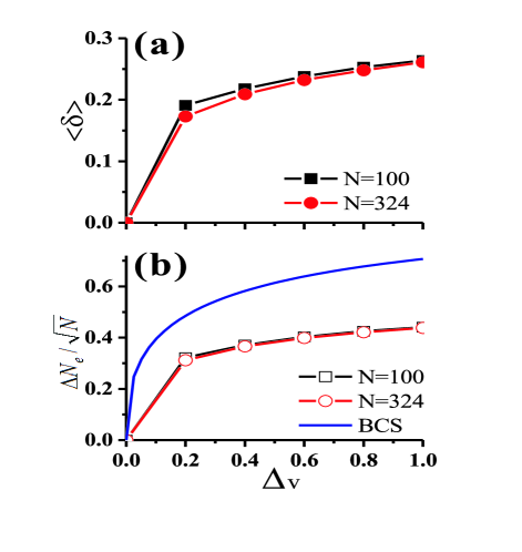
Figure 1: (Color online) (a) The average doping density and (b) its fluctuation as a function of the variational parameter $\Delta_{v}$ for the wave function of Eq.(9) using the BCS coherence factors. Results for a cluster of $10\times 10$ and $18\times 18$ are shown in black and red, respectively. Other parameters are set to be $\mu_{v}=t_{v}^{\prime}=t_{v}^{\prime\prime}=0$. The blue line in (b) is the $d$-wave BCS result.

We can further study Eq.(13) by carrying out the numerical calculation using the VMC method. We consider the simple BCS wave function by replacing $\tilde{u}_{\mathbf{k}}$ and $\tilde{v}_{\mathbf{k}}$ in Eq.(9) with $u_{\mathbf{k}}$ and $v_{\mathbf{k}}$, respectively. $u_{\mathbf{k}}$ and $v_{\mathbf{k}}$ are the BCS coherence factors, defined by

$$u_{k} = \sqrt{\frac{1}{2}\left(1+\frac{\epsilon_{k}}{\sqrt{\epsilon_{k}^{2}+\Delta_{k}^{2}}}\right)},$$

$$v_{k} = Sgn(\Delta_{k})\sqrt{\frac{1}{2}\left(1-\frac{\epsilon_{k}}{\sqrt{\epsilon_{k}^{2}+\Delta_{k}^{2}}}\right)},$$ (14)

where

$$\epsilon_{k} = -2\left(cosk_{x}+cosk_{y}\right)-4t_{v}^{\prime}cosk_{x}cosk_{y}$$

$$-2t_{v}^{\prime\prime}\left(cos2k_{x}+cos2k_{y}\right)-\mu_{v},$$

$$\Delta_{k} = 2\Delta_{v}\left(cosk_{x}-cosk_{y}\right).$$ (15)

Here $\Delta_{v}$, $\mu_{v}$, $t_{v}^{\prime}$, and $t_{v}^{\prime\prime}$ are variational parameters. For illustration we will consider the half-filling wave function with the variational parameters: $\mu_{v}=t_{v}^{\prime}=t_{v}^{\prime\prime}=0$. The only parameter left is $\Delta_{v}$ which varies from $0$ to $1$. In Fig.1(a) and (b), we show the average doping density $\langle\delta\rangle(\equiv 1-N_{e}/N)$ and the particle number fluctuation $\Delta N_{e}/\sqrt{N}$ as a function of $\Delta_{v}$, respectively. The result of the $d$-wave BCS state without projection is also shown in Fig.1(b). Clearly as discussed above the introduction of projection has greatly changed the distribution function of particle number with a larger average doping density and smaller fluctuation.

Now we can construct the $d$-RVB wave function in the grand-canonical ensemble by taking into account this change of distribution function. Eq.(12) suggests that the important doping dependence of the distribution function in the presence of the Gutzwiller projection operator $\hat{P}_{G}$ is the factor $g^{-\hat{N}_{h}}$, where $g\equiv\frac{2\delta}{1+\delta}$, $\hat{N}_{h}=N-\hat{N}_{e}$, and $\hat{N}_{e}=\sum_{i,\sigma}\hat{c}_{i\sigma}^{{\dagger}}\hat{c}_{i\sigma}$. The operator $g^{-\hat{N}_{h}}$ mimicking the effect of $\hat{P}_{G}$ tends to increase the doping density away from half-filling. To balance this effect, we have to place the operator $\sqrt{g}^{\hat{N}_{h}}$ in front of the $d$-RVB wave function. Thus, the $d$-RVB state in the grand-canonical scheme can be written as

$$|\Psi_{d-RVB}^{g}\rangle = \hat{P}_{G}\sqrt{g}^{\hat{N}_{h}}\prod_{\mathbf{k}}\left(u_{\mathbf{k}}+v_{\mathbf{k}}\hat{c}^{\dagger}_{\mathbf{k}\uparrow}\hat{c}^{\dagger}_{-\mathbf{k}\downarrow}\right)|0\rangle_{(c)}$$ (16)

$$\rightarrow \hat{P}_{G}\prod_{\mathbf{k}}\left(gu_{\mathbf{k}}\hat{d}^{\dagger}_{\mathbf{k}}+v_{\mathbf{k}}\hat{f}^{\dagger}_{\mathbf{k}}\right)|0\rangle_{(df)}$$

$$\equiv \hat{P}_{G}|\Psi_{d-BCS}^{g}\rangle.$$

Now $g$ can be seen as a variational parameter like $\mu_{v}$, $t_{v}^{\prime}$, $t_{v}^{\prime\prime}$, and $\Delta_{v}$. Eq.(16) with the fugacity factor is exactly the wave function proposed by Anderson AndersonJPCS06 and Laughlin LaughlinPM06 . Previously the fugacity factor $g$ was estimated to be $\frac{2\delta}{1+\delta}$ by using GA.

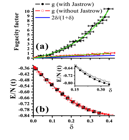
Figure 2: (Color online) The doping dependence of (a) the variational parameter $g$ and (b) the optimized energy per site for a $12\times 12$ lattice. In (a), Solid (Empty) circles indicate the fugacity factors $g$ with (without) Jastrow factors. The blue line shows the renormalized Gutzwiller’s factor $\frac{2\delta}{1+\delta}$. The green lines are the guide to the eyes. In (b), black squares (Red circles) indicate the $d$-RVB wave function with Jastrow factors in the (grand-) canonical ensemble. Error bars represent the average density. Inset: Solid (Empty) squares represent the $d$-RVB wave function with (without) Jastrow factors in the canonical ensemble. The bare parameters in the Hamiltonian are set to be $(t^{\prime},t^{\prime\prime},J)/t=(-0.3,0.15,0.3)$.

To obtain the ground state in the grand-canonical case, we have to optimize the grand thermodynamic potential $F=E-\mu_{g}N_{e}$ instead of the internal energy $E$ with a fixed chemical potential $\mu_{g}$. Here $N_{e}$ is the average number of electrons for each $\mu_{g}$. Notice that $\mu_{g}$ is different from the variational parameter $\mu_{v}$ in the $d$-RVB wave function. To have a lower ground-state energy, for all the numerical results discussed below we consider a modified $d$-RVB wave function $\hat{P}_{J}|\Psi_{d-RVB}^{g}\rangle$ where we introduce a hole-hole repulsive Jastrow factor $\hat{P}_{J}$ HellbergPRL91 ; ValentiPRL92 ; SorellaPRL02 ; CPChouPRB08 :

$$\hat{P}_{J}=\prod_{i<j}\left[1-\left(1-r_{ij}^{\alpha}v_{\beta}^{\delta_{j,i+\beta}}\right)\hat{n}_{i}^{h}\hat{n}_{j}^{h}\right]$$ (17)

with

$$r_{ij}=\sqrt{\sin^{2}\left(\frac{\pi}{L}(x_{i}-x_{j})\right)+\sin^{2}\left(\frac{\pi}{L}(y_{i}-y_{j})\right)}.$$ (18)

Here $\hat{n}_{i}^{h}=1-\sum_{\sigma}c_{i\sigma}^{{\dagger}}c_{i\sigma}$. The three parameters $v_{\beta}$ with $\beta$ to be the nearest, second nearest, and third nearest neighbors are for short-range hole-hole repulsion if these values are less than 1. The factor $r_{ij}^{\alpha}$ is for long-range correlations and it is repulsive if $\alpha$ is positive. $L$ is the linear scale of the lattice. In Fig.2(a), we obtain the doping dependence of the fugacity factor $g$ from the grand-thermodynamic-potential optimization. Interestingly, since Jastrow factors will reduce the probability that holes come closer, the fugacity factor of the modified $d$-RVB state is greatly enhanced as increasing doping. If we do not consider Jastrow factors, the doping dependence of $g$ is similar to the renormalized Gutzwiller’s factor $2\delta/(1+\delta)$. Therefore, although the GA result is not exact, it is a reasonable approximation.

IV Quasi-particle Energy Dispersion and Spectral Weight

In Fig.2(b), the optimized internal energy per site is plotted as a function of the doping density for both canonical (black squares) and grand canonical (red circles) cases. The results are essentially indistinguishable for a $12\times 12$ lattice. Thus the ground-state phase diagram obtained in the canonical ensemble ShihPRL04 ; KYYangPRB06 will be essentially the same as the grand-canonical scheme. This result is expected as the calculation of internal energy only involves states with the same number of particles AndersonIJMPB11 . Additionally, the energies obtained with the Jastrow factor are quite lower than without the factors for the canonical case, as shown in the inset of Fig.2(b). The fugacity factor $g$ of the modified $d$-RVB state is very different from the case without Jastrow factors shown in Fig.2(a).

It should be noted that we can also use the results in Fig.2(b) obtained by Eq.(1) to calculate the relation between chemical potential and average number of particles as $\mu_{g}\equiv\partial E/\partial N_{e}$. Completely consistent results are obtained. The excellent agreement between the energies calculated by the grand-canonical and canonical schemes is the most important numerical result of this paper to firmly establish the validity of inclusion of the fugacity factor $g$ in Eq.(16) and our Monte Carlo algorithm. Now we can start to calculate excitation spectra and other physical quantities in the grand-canonical ensemble.

Not only we shall consider the energy dispersion of the excitations but also the spectral weight below. These results could be compared with the measured STS. The simplest way to construct a single-particle excitation from the $d$-RVB state is to bring the quasi-particle creation operator $\tilde{\gamma}_{k\sigma}^{{\dagger}}(=\frac{gu_{k}}{\sqrt{(gu_{k})^{2}+v_{k}^{2}}}c_{k,\sigma}^{{\dagger}}-\frac{v_{k}}{\sqrt{(gu_{k})^{2}+v_{k}^{2}}}c_{-k,-\sigma})$ into play,

$$|\Psi_{k\sigma}^{g}\rangle=\hat{P}_{G}\tilde{\gamma}_{k\sigma}^{{\dagger}}|\Psi_{d-BCS}^{g}\rangle.$$ (19)

Excitation energies cannot be calculated from the internal energy difference $E_{k}-E_{0}$ as in the canonical ensemble CPChouPRB06 , where $E_{0}$ is the ground-state energy. Here the chemical potential is fixed, hence we must calculate the grand thermodynamic potential for the ground state and excited states, $F_{0}$ and $F_{k}$, respectively,

$$F_{0} = \langle\Psi_{d-RVB}^{g}|\hat{H}-\mu_{g}\hat{N}_{e}|\Psi_{d-RVB}^{g}\rangle,$$

$$F_{k} = \langle\Psi_{k\sigma}^{g}|\hat{H}-\mu_{g}\hat{N}_{e}|\Psi_{k\sigma}^{g}\rangle.$$ (20)

It is noticed that due to the BCS coherence factors $u_{k}$ and $v_{k}$, the excited state $|\Psi_{k\sigma}^{g}\rangle$ will have fewer (more) average particle numbers below (above) the Fermi level than the ground state $|\Psi_{d-RVB}^{g}\rangle$ (not shown). Here we have made an important assumption that these particular states Eq.(19) have little overlap with other states with same momentum and spin. This is probably valid for low-energy excitations less than the gap energy.

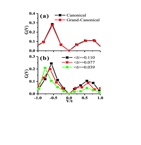
Figure 3: (Color online) $G(V)$ for the $d$-RVB state versus the bias $V$. (a) Canonical (Grand-canonical) results for hole doping $\delta$ (chemical potential $\mu_{g}$) fixed to $0.125$ ($1.68t$) in $12\times 12$ lattice. (b) Grand canonical results for three chemical potentials $\mu_{g}$, $1.68t$ (black-squares), $1.9t$ (red-circles), and $2.1t$ (green-triangles). $V$ is negative (positive) for removing (adding) one electron in $20\times 20$ lattice. The bare parameters in the Hamiltonian are set to be $(t^{\prime},t^{\prime\prime},J)/t=(-0.3,0.15,0.3)$.

The above quasi-particle states are then used to calculate the spectral weight for adding (removing) one electron with momentum $k$ ($-k$) and spin $\sigma$ ($-\sigma$) to the ground state as defined

$$Z_{k,\sigma(-k,-\sigma)}^{+(-)}=\frac{\left|\langle\Psi_{k\sigma}^{g}|c_{k,\sigma}^{{\dagger}}(c_{-k,-\sigma})|\Psi_{d-RVB}^{g}\rangle\right|^{2}}{\langle\Psi_{d-RVB}^{g}|\Psi_{d-RVB}^{g}\rangle\langle\Psi_{k\sigma}^{g}|\Psi_{k\sigma}^{g}\rangle}.$$ (21)

Similar to what we have done for the canonical case CPChouPRB06 , we could also calculate the tunneling conductance for the grand-canonical wave function with the bias given by $V=F_{k}-F_{0}$. For the numerical calculations, we define the tunneling conductance as

$$G(V)=\frac{1}{N\Delta F}\sum_{k\in V\pm\Delta F/2}Z_{\pm k,\pm\sigma}^{\pm},$$ (22)

where $\Delta F=0.28t\ (0.2t)$ for $N=144\ (400)$ chosen is to reduce the effect due to the finite lattice size and $\sigma$ either up or down spin. Similar to Fig.2(b), Fig.3(a) also shows except for high voltage the tunneling conductances are almost identical in the canonical and the grand-canonical ensemble. Once again, the equivalence between the canonical and the grand-canonical ensemble for the excitation spectra within the gap convinces us of the conclusion that the modified $d$-RVB wave function with the fugacity factor is the precise representation for the RVB-type state in the grand-canonical case.

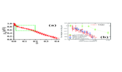
Figure 4: (Color online) (a) The doping dependence of chemical potential $\mu_{g}$ in a $12\times 12$ lattice. Red circles represent the $d$-RVB state with Jastrow factors in the grand-canonical ensemble. Error bars indicate $\Delta N_{e}/N$ at each average doping. (b) The doping dependence of chemical-potential shift from experiments in several cuprate materials HashimotoPRB08 compared with the region shown by the green-dashed frame in (a). Red empty circles in (b), shifted along the vertical direction for comparison, are the data from the green-dashed frame in (a). The bare parameters in the Hamiltonian are set to be $(t^{\prime},t^{\prime\prime},J)/t=(-0.3,0.15,0.3)$. Here $t$ is set to be $0.4eV$.

In addition, to numerically examine the particle-hole asymmetry of tunneling spectra in the grand-canonical ensemble, we present the doping dependence of $G(V)$ in Fig.3(b). The asymmetry is clearly observed for all three doping densities. At $\delta=0.039$, the total spectral weight for removing one electron, defined as the sum of $Z_{k\sigma}^{-}$ over the Brillouin zone, is found to be about three times as large as the one for adding one electron. The gap value deduced from the width between peak positions decreases with doping. Note that the gap size is usually overestimated in the extended $t-J$ models. However, the weight value obtained from the peak height enhances as increasing doping, apparently anticorrelating with the gap size. All of these features have been shown in the canonical ensemble CPChouPRB06 and qualitatively consistent with the STS measurements GomesNat07 ; PushpSci09 . Although the details of the tunneling spectra in Ref. AndersonLTP06, is not completely identical to that shown in Fig.3(b), their important characteristics are similar.

V Chemical Potential

The doping dependence of $\mu_{g}$ calculated in the grand-canonical ensemble is plotted in Fig.4(a). It decreases monotonically with doping as expected from Fig.4(b). Near half-filling, $\mu_{g}$ seems to increase greatly. The compressibility becomes extremely small as electron density approaches half filling, this is a consequence of the opening of a charge gap of a Mott insulator. This behavior was also observed in the calculation of Yokoyama and Shiba YokoyamaJPSJ88 . But the quantitative behavior is different as the fugacity factor was not included in their grand-canonical wave function. We have also examined the doping dependence of $\mu_{g}$ for several bare parameters $t^{\prime}/t$. The slopes for all $t^{\prime}/t$ are similar except for very large doping (not shown). Here, only the relative value of $\mu_{g}$ is meaningful. Thus we can shift $\mu_{g}$ to compare with experiments. Figure 4(b) shows chemical-potential shift for several cuprates observed by photoemission experiments HashimotoPRB08 . Except for $La-214$ samples the slope of chemical potential as a function of $\delta$ obtained by our calculation (see the green-dashed frame in Fig.4(a)) is almost identical to the experimental data. This result is more quantitatively reliable in comparison with the experiments than our previous studies in the canonical ensemble KYYangPRB06 in the low doping region. As for the inconsistency with $La-214$ cuprates, a possible reason could be the existence of stripe order in those materials ZaanenAP96 ; InoPRL97 . It will be interesting to investigate chemical-potential shift by using the Gutzwiller-projected stripe wave function CPChouPRB10 in the grand-canonical ensemble in the future.

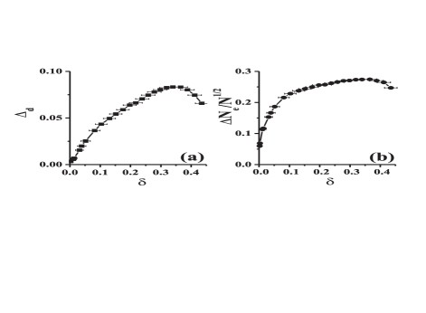
Figure 5: The doping dependence of (a) the SC order parameter $\Delta_{d}$ and (b) the scaled particle number fluctuation $\Delta N_{e}/\sqrt{N}$ using the $d$-RVB state in the $12\times 12$ lattice in the grand-canonical ensemble. Error bars indicate $\Delta N_{e}/N$ at each average doping. The bare parameters in the Hamiltonian are set to be $(t^{\prime},t^{\prime\prime},J)/t=(-0.2,0.1,0.3)$.

VI SC Order Parameter and Particle Number Fluctuation

In order to investigate the SC characteristics of the $d$-RVB wave function, we calculate the SC order parameter $\Delta_{d}$ and the particle number fluctuation $\Delta N_{e}$ impossible to be derived in the canonical ensemble, as shown in Fig.5(a) and (b), respectively. The SC order parameter $\Delta_{d}$ which is presumably proportional to the SC critical temperature $T_{c}$ is plotted as a function of doping density in Fig.5(a). The dome-like shape comparable to the SC phase in the cuprate phase diagrams is consistent with earlier VMC results in the canonical ensemble CPChouPRB06 . The density with the maximum value of order parameter is again much larger than the optimal doping density in cuprates. In the BCS theory the fluctuation of the particle number, $\Delta N_{e}$, is proportional to the SC order parameter. In Fig.5(b), $\Delta N_{e}/\sqrt{N}$ is plotted as a function of doping density. Comparison between Fig.5(a) and (b) shows that both $\Delta N_{e}$ and $\Delta_{d}$ calculated by using the $d$-RVB state have the similar dome-like shape, but there is a significant difference at underdoped regime. This difference is clearly due to the projection operator or the Mott physics as the particle number fluctuation is suppressed for low doping.

VII Phase Fluctuation

Before looking into the phase fluctuation $\Delta\Theta$ of the $d$-RVB wave function, we shall start with the $d$-wave BCS state at first. To obtain useful information about the phase of wave functions, a ”phase” operator is defined by

$$\hat{\Theta}=\frac{\hat{\Delta}-\hat{\Delta}^{{\dagger}}}{2i\Delta_{0}},$$ (23)

where $\hat{\Delta}^{{\dagger}}\equiv\sum_{k}\varphi_{k}c_{k\uparrow}^{{\dagger}}c_{-k\downarrow}^{{\dagger}}$ and the normalization $\Delta_{0}=|\langle\hat{\Delta}^{{\dagger}}\rangle|$. Here we choose $\varphi_{k}=\langle c_{k\uparrow}^{{\dagger}}c_{-k\downarrow}^{{\dagger}}\rangle$. Hence, any real wave function will lead to $\langle\hat{\Theta}\rangle=0$. With a little algebra, it is straight forward to write down the particle number fluctuation $\Delta N_{e}$ and the phase fluctuation $\Delta\Theta$ of the BCS state as

$$\Delta N_{e} = 2\sqrt{\sum_{k}|u_{k}|^{2}|v_{k}|^{2}},$$

$$\Delta\Theta = \frac{\sqrt{\sum_{k}\varphi_{k}^{2}}}{2\sum_{k}\varphi_{k}|u_{k}||v_{k}|}.$$ (24)

Then the uncertainty principle for particle number and phase can be easily derived by Cauchy-Schwarz inequality:

$$\Delta N_{e}\Delta\Theta=\sqrt{\frac{\sum_{k}\varphi_{k}^{2}\cdot\sum_{k}|u_{k}|^{2}|v_{k}|^{2}}{\left(\sum_{k}\varphi_{k}|u_{k}||v_{k}|\right)^{2}}}\geq 1.$$ (25)

It can be proved that $\Delta N_{e}\Delta\Theta$ in terms of the definition of Eq.(23) is exactly equal to 1 in BCS theory. The doping dependence of the particle number fluctuation and the phase fluctuation in the $d$-wave BCS case are shown in Fig.6(a).

Although it is impossible to evaluate the phase fluctuation for the wave function of Eq.(1) with a fixed number of particles, it is straight forward for the $d$-RVB wave function by calculating the following quantity

$$\Delta\Theta \equiv \sqrt{\left\langle\left(\hat{\Theta}-\left\langle\hat{\Theta}\right\rangle\right)^{2}\right\rangle}$$ (26)

$$= \sqrt{\frac{\langle\Psi_{d-RVB}^{g}|\hat{\Delta}^{{\dagger}}\hat{\Delta}-\hat{\Delta}^{{\dagger}}\hat{\Delta}^{{\dagger}}|\Psi_{d-RVB}^{g}\rangle}{2\Delta_{0}^{2}}}.$$

In addition to $\Delta_{0}$, there are two quantities to be calculated by means of the VMC approach: one is the pairing correlation operator $\hat{\Delta}^{{\dagger}}\hat{\Delta}$ and the other $\hat{\Delta}^{{\dagger}}\hat{\Delta}^{{\dagger}}$. Using the representation (df), we can calculate both quantities directly.

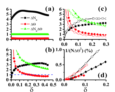
Figure 6: The doping dependence of the particle number fluctuation $\Delta N_{e}$, the phase fluctuation $\Delta\Theta$, and their product using (a) the $d$-wave BCS state and (b) the $d$-RVB state with Jastrow factors in the grand-canonical ensemble. The $d$-wave BCS state is obtained by solving the BCS Hamiltonian with bare parameters $(t^{\prime},t^{\prime\prime},V)/t=(-0.2,0.1,6)$ self-consistently. $V$ is the pairing interaction strength. The blue dashed line denotes 1. (c) The doping dependence of $\Delta N_{e}$ (squares), $\Delta\Theta$ (circles), and $\Delta N_{e}\Delta\Theta$ (triangles) using the $d$-RVB state with (filled) and without (empty) Jastrow factors. (d) The doping dependence of $\frac{1}{\Delta\Theta^{2}N}$ with (filled diamonds) and without (empty diamonds) Jastrow factors. Black (Red) color indicates $N=144\ (256)$. All the results are obtained with parameters $(t^{\prime},t^{\prime\prime},J)/t=(-0.2,0.1,0.3)$ for a $12\times 12$ lattice except specially mentioned results in (d).

In Fig.6(b), we show the doping dependence of the particle number fluctuation and the phase fluctuation using the $d$-RVB wave function. As mentioned before, the Gutzwiller projection operator $\hat{P}_{G}$ suppresses the particle number fluctuation as shown in Fig.6(b), especially for the underdoped region. On the other hand, the phase fluctuation is greatly enhanced for $0<\delta<0.15$, and a much weaker dependence for doping greater than $0.15$. Although the fluctuation behavior is approaching BCS results in the overdoped region, it is still much stronger. This huge enhancement of $\Delta\Theta$ is clearly due to the strong correlation effect of the Gutzwiller projection operator. This result suggests that there may exist a strong phase-fluctuating state which is again consistent with experiments in the underdoped cuprate compounds YWangPRB06 ; LeeSci09 and a theoretical analysis TesanovicNP08 . Another interesting result is the large enhancement of $\Delta N_{e}\Delta\Theta$. Instead of having the value of $1$ as the BCS state, it seems to approach infinity at very low doping. This is mainly due to the strong increase of phase fluctuation as doping decreases.

Fig.6(c) shows the doping dependence of $\Delta N_{e}$ (squares), $\Delta\Theta$ (circles), and $\Delta N_{e}\Delta\Theta$ (triangles) using the $d$-RVB state with (filled) and without (empty) Jastrow factors. As discussed before, the Jastrow factor suppresses the number fluctuation, hence it increases the phase fluctuation. But the substantial increase of the phase fluctuation at low doping region is quite surprising since the energy difference between these two states is quite small as shown in the inset of Fig.2(b). Their product $\Delta N_{e}\Delta\Theta$ for the case with Jastrow factors also deviates farther from 1 near the underdoped regime. It indicates that the system in the underdoped region may have many low energy states with similar energy but different properties.

In Fig.6(d), we find that the doping dependence of $\frac{1}{\Delta\Theta^{2}N}$ exhibits approximately a linear relation, shown by the empty diamonds, within $0.03<\delta<0.25$ for the $d$-RVB state without including the Jastrow factor. Due to the finite size, it is difficult to get reliable results at extremely low density but the results of two different cluster sizes are consistent. This result is in sharp contrast with BCS theory which has $\frac{1}{\Delta\Theta^{2}N}$ proportional to the pairing gap instead of the doping density. After the Jastrow factor is included, as shown by the filled diamonds in Fig.6(d), phase fluctuation is enhanced. However, the linear dependence of doping density at low density still remains but with a smaller slope.

Empirically the superfluid density of the hole-doped cuprates is small and proportional to the doping density UemuraSSC03 . For a SC state the phase stiffness is proportional the superfluid density. Although we do not have a direct proof of the relation between phase stiffness and $\frac{1}{\Delta\Theta^{2}N}$, it is quite interesting that they both are proportional to the doping density. In addition, the slope for the wave function with the Jastrow factor is smaller than the one without the Jastrow factor, which may indicate that the SC ground state of the $t-J$ model will have a very small superfluid density just as the hole-doped cuprates.

VIII Conclusions

To summarize, we have studied the properties of the ground state and Bogoliubov quasi-particle states in the extended $t-J$ model based on Gutzwiller-projected BCS wave function or $d$-RVB wave function in the grand-canonical ensemble. First of all, by using the phase space argument used in GA EdeggerPRB05 , we have numerically demonstrated how to construct the correct $d$-RVB wave function with non-conserving particle numbers. A fugacity factor $g$ in front of $u_{k}$ in the $d$-RVB state is able to efficiently govern the distribution of empty sites. Our numerical calculations have shown the excellent agreement obtained for both the optimized grand thermodynamic potential and tunneling spectra $G(V)$ between the grand-canonical and the canonical ensemble. It confirms the necessity and importance of the fugacity factor $g$ in the $d$-RVB state in the grand-canonical ensemble as emphasized by Anderson AndersonLTP06 . The enhanced tunneling asymmetry at low voltage in the underdoped region is again numerically demonstrated.

In addition, as increasing doping, chemical potential $\mu_{g}$ calculated in the grand-canonical scheme monotonically declines with the slope which is in good agreement with the experimental results HashimotoPRB08 . Almost zero charge susceptibility near half-filling indicates the incompressible feature due to the Mott gap. Both the SC order parameter and the particle number fluctuation have the dome-like doping dependence similar to the SC dome in high-$T_{c}$ phase diagrams. The doping dependence of the SC order parameter is similar to that of the particle number fluctuation for large doping density as the BCS theory. But for low doping density, there is a significant difference due to the Gutzwiller projection operator. Furthermore, now we are able to directly calculate the phase fluctuation in the grand-canonical ensemble. The Gutzwiller-projected wave function shows not only the smaller particle number fluctuation but the much enhanced phase fluctuation than the wave function without Gutzwiller projection in the underdoped region. We also found $\Delta N_{e}\Delta\Theta$ much greater than $1$.

In this paper, we only used a uniform fugacity factor in the $d$-RVB states. Without including a Jastrow factor to obtain a lower energy, this factor is close to the derived results of GA. However, including the Jastrow factor produces a much larger fugacity factor and a significantly enhanced phase fluctuation. This indicates that the fugacity factor may be quite important in the underdoped region. In addition, the fugacity factor could have a spatial dependence or a momentum dependence as noticed by Anderson AndersonIJMPB11 . The spatial dependence could produce the stripes as we demonstrated in Refs. CPChouPRB08, and  CPC2011, that the Gutzwiller projection operator introduces the coupling between charge density, spin density and pair fields. The effect of the momentum dependence will be left for future study.

^∗yangfan_blg@bit.edu.cn

References

- (1) P. W. Anderson, Science 235, 1196 (1987).
- (2) P. W. Anderson and N. P. Ong, J. Phys. Chem. Solids 67, 1 (2006).
- (3) P. W. Anderson, Low Temp. Phys. 32, 282 (2006).
- (4) R. B. Laughlin, Philos. Mag. 86, 1165 (2006).
- (5) B. Edegger, N. Fukushima, C. Gros, and V. N. Muthukumar, Phys. Rev. B 72, 134504 (2005).
- (6) P. W. Anderson, P. A. Lee, M. Randeria, T. M. Rice, N. Trivedi, and F. C. Zhang, J. Phys.: Condens. Matter 16, R755 (2004).
- (7) H. Yokoyama and H. Shiba, J. Phys. Soc. Japan 56, 3570 (1987).
- (8) C. Gros, Phys. Rev. B 38, 931 (1988).
- (9) B. Edegger, V. N. Muthukumar and C. Gros, Advances in Physics 56, 927 (2007).
- (10) A. Paramekanti, M.Randeria, and N. Trivedi, Phys. Rev. B 70, 054504 (2004).
- (11) C.T. Shih, T.K. Lee, R. Eder, C.Y. Mou and Y.C. Chen, Phys. Rev. Lett. 92, 227002 (2004).
- (12) Kai-Yu Yang, C. T. Shih, C.-P. Chou, S. M. Huang, T. K. Lee, T. Xiang, and F. C. Zhang, Phys. Rev. B 73, 224513 (2006).
- (13) H. Yokoyama and M. Ogata, J. Phys. Soc. Japan 65, 3615 (1996).
- (14) C. T. Shih, Y. C. Chen, C. P. Chou, and T. K. Lee, Phys. Rev. B 70, 220502 (2004).
- (15) C. T. Shih et al., Low Temp. Phys. 31, 757 (2005).
- (16) A. Himeda and M. Ogata, Phys. Rev. B 60, R9935 (1999).
- (17) C.-P. Chou, N. Fukushima, and T.-K. Lee, Phys. Rev. B 78, 134530 (2008).
- (18) C.-P. Chou and T.-K. Lee, Phys. Rev. B 81, 060503(R) (2010).
- (19) A. Himeda, T. Kato, and M. Ogata, Phys. Rev. Lett. 88, 117001 (2002).
- (20) M. Randeria, A. Paramekanti, and N. Trivedi, Phys. Rev. B 69, 144509 (2004).
- (21) S. Yunoki, E. Dagotto, and S. Sorella, Phys. Rev. Lett. 94, 037001 (2005); S. Yunoki, Phys. Rev. B 72, 092505 (2005); S. Yunoki, Phys. Rev. B 74, 180504(R)(2006).
- (22) C. P. Nave, D. A.Ivanov, and P. A. Lee, Phys. Rev. B 73, 104502 (2006).
- (23) C.-P. Chou, T. K. Lee, and C.-M. Ho, Phys. Rev. B 74, 092503 (2006).
- (24) H.-Y. Yang, F. Yang, Y.-J. Jiang, and T. Li, J. Phys.: Condens. Matter 19, 016217 (2007).
- (25) H. Yokoyama and H. Shiba, J. Phys. Soc. Jpn. 57, 2482 (1988).
- (26) C. Renner and Ø. Fischer, Phys. Rev. B 51, 9208 (1995).
- (27) T. Hanaguri et al., Nature 430, 1001 (2004).
- (28) K. McElroy et al., Phys. Rev. Lett. 94, 197005 (2005).
- (29) A. C. Fang et al., Phys. Rev. Lett. 96, 017007 (2006).
- (30) M. Hashimoto et al., Phys. Rev. B 77, 094516 (2008).
- (31) C. Gros, Ann. Phys. (N.Y.) 189, 35 (1989).
- (32) P. W. Anderson, Int. J. Mod. Phys. B 25, 1 (2011).
- (33) C. S. Hellberg and E. J. Mele, Phys. Rev. Lett. 67, 2080 (1991).
- (34) R. Valenti and C. Gros, Phys. Rev. Lett. 68, 2402 (1992).
- (35) S. Sorella, G. B. Martins, F. Becca, C. Gazza, L. Capriotti, A. Parola, and E. Dagotto, Phys. Rev. Lett. 88, 117002 (2002).
- (36) K. K. Gomes et al., Nature 447, 569 (2007).
- (37) A. Pushp et al., Science 324, 1689 (2009).
- (38) J. Zaanen and A. M. Oleá, Ann. Phys. (Leipzig) 5, 224 (1996).
- (39) A. Ino et al., Phys. Rev. Lett. 79, 2101 (1997).
- (40) Y. Wang, L. Li, and N. P. Ong, Phys. Rev. B 73, 024510 (2006).
- (41) J. Lee et al., Science 325, 1099 (2009).
- (42) Z. Tesanovic, Nature Physics 4, 408 (2008).
- (43) Y. J. Uemura, Solid State Comm. 126, 23 (2003).
- (44) C.-P. Chou and T. K. Lee, to be submitted.