Stability of linear and non-linear lambda and tripod systems in the presence of amplitude damping

Abstract

We present the stability analysis of the dark states in the adiabatic passage for the linear and non-linear lambda and tripod systems in the presence of amplitude damping (losses). We perform an analytic evaluation of the real parts of eigenvalues of the corresponding Jacobians, the non-zero eigenvalues of which are found from the quadratic characteristic equations, as well as by the corresponding numerical simulations. For non-linear systems, we evaluate the Jacobians at the dark states. Similarly to the linear systems, here we also find the non-zero eigenvalues from the characteristic quadratic equations. We reveal a common property of all the considered systems showing that the evolution of the real parts of eigenvalues can be split into three stages. In each of them the evolution of the stimulated Raman adiabatic passage (STIRAP) is characterized by different effective dimension. This results in a possible adiabatic reduction of one or two degrees of freedom.

1 Introduction

Over the last couple of decades there has been a continuing interest in the stimulated Raman adiabatic passage (STIRAP) [1, 2, 3, 4, 5]. The simplest situation is the adiabatic passage in a linear lambda system [6, 7, 8, 9, 10, 11, 12] containing a single dark (uncoupled) state which is immune to the atom-light coupling. If atomic initial and final states are the ground states representing the dark states of the system, the atom can be transferred between these two states by slowly changing the relative intensity of the laser pulses. When the adiabatic passage is slow enough, the excited state is only slightly populated and thus the losses are minimum. The analysis has been extended for the STIRAP process in the tripod system characterized by two dark states [13, 14, 15]. This enables to create a quantum superposition of metastable states out of a single initial state in a robust and coherent way [16, 17]. The schemes involving more atomic and molecular levels were also proposed for creation a superposition of states [18] as well as for experimental control of excitation flow [19]. Recently the treatment was further extended to the non-linear lambda [20, 21, 22, 23, 24, 25, 26, 27, 28, 29, 30, 31] and tripod [32] schemes.

Usually the STIRAP is based on the adiabatic approximation. However, one has to distinguish between the adiabatic approximation and the adiabatic reduction of dynamic systems. In quantum mechanics, a closed quantum system is said to undergo adiabatic dynamics if its Hilbert space can be decomposed into decoupled Schrödinger eigenspaces with distinct, time-continuous, and non-crossing instantaneous eigenvalues of Hamiltonian. On the other hand an open quantum system is said to undergo adiabatic dynamics if its Hilbert-Schmidt space can be decomposed into decoupled Lindblad-Jordan eigenspaces with distinct, time-continuous, and non-crossing instantaneous eigenvalues of the Lindblad superoperator [33]. The system is called adiabatically approximated if the error term in the Schrödinger equation (for closed systems) or in the master equation (for open systems) is much less than the diagonalysed part; i.e. one may neglect the non-diagonal terms in order to get an adiabatically approximated version of the system. Note that in the presence of fast driven oscillations some additional conditions (in addition to the slowness of the evolution of the Hamiltonian) have to be imposed [34].

Another procedure is the adiabatic elimination of decaying degrees of freedom. It is related to the dynamic systems in which some degrees of freedom may decay. In accordance with this definition, these degrees of freedom may be adiabatically eliminated by solving the corresponding algebraic equations; the r.h.s. of decaying equations are set to be equal to zero. Consequently, one obtains the dependencies of decaying variables on the remaining ones. If there are several decaying variables, one may eliminate them one by one, starting from the fastest variable, and finishing with the slowest one. Such a procedure can be found e.g. in the book by Haken [35].

The aim of the present work is to perform a stability analysis of the dark states in the adiabatic passage for the linear and non-linear lambda and tripod systems. The analysis sets limits to the adiabatic reduction of the systems. Moreover, we have revealed that in all the considered systems, the stability properties of the dark states are similar, namely, there are three time intervals with different number of the negative real parts of the Jacobians. This suggests that the corresponding linear and non-linear systems have equal possibilities of adiabatic reduction. Although the linear lambda [1, 2, 3, 4, 5, 6, 7, 8, 9, 10, 11, 12] and tripod systems [13, 14, 15, 16, 17, 36] have been substantially studied in the literature, here we apply our treatment also to these linear setups in order to facilitate the subsequent analysis of the non-linear systems.

The non-linear lambda system can be realized in the Bose-Einstein condensates (BEC) via photoassociation (PA) from a dissociated (quasicontinuum) atomic state to the ground molecular state in the presence of the intermediate molecular state [20, 21]. The aim of the quantum control is to transfer the whole population from the dissociated atomic to the ground molecular state. One thus creates ultracold molecules by associating cold atoms [29, 37]. In this case the dark state is a generalisation of that for the linear systems. In the linear case, the dark state is defined as a superposition of the initial and target ground atomic states which corresponds to the zero eigenergy of the system Hamiltonian. The same dark state may be also defined as a steady state solution of the Schrödinger equation. If we consider the nonlinear system, we can again define the dark state as a steady state [29] of the equations of motion following from the Heisenberg equation. In the nonlinear systems, the behaviour of the dark state reproduces that in the linear systems although the superposition is missing now. We thus get the nonlinear version of STIRAP: the entire population is distributed among the steady state probability amplitudes of the initial atomic and the target molecular state. At the beginning the whole population is atomic, whereas at the end it is in the ground molecular state.

Differently from the traditional STIRAP in an atomic lambda system, the atom-molecule STIRAP contains nonlinearities originating from the conversion process of atoms to molecules, as well as from the interparticle interactions described by the non-linear mean-field contributions. The existence of such nonlinearities makes it difficult to analyse the adiabaticity of the atom-molecule conversion systems due to the absence of the superposition principle. In the STIRAP, the linear instability could make the quantum evolution deviate from the dark state rapidly even in adiabatic limit [22]. Therefore, it is important to avoid such an instability for the efficiency of the STIRAP.

The non-linear tripod system can be realized in the PA with two target states involved. Specifically, one may consider the atom-molecule transition in ultracold quantum gases via PA. It was first considered in [32] where the second order dynamic system was derived that parametrizes the solution evolving on the dark state manifold. However the stability of the solution moving along the manifold was not considered. Therefore we shall check the stability of this solution, i.e. see whether the nearby solutions are attracted back to this manifold.

The adiabatic theory for non-linear quantum systems was first discussed by Liu et al. [38] who obtained the adiabatic conditions and adiabatic invariants by representing the non-linear Heisenberg equation in terms of an effective classical Hamiltonian. Pu et al. [23] and Ling et al. [24] extended such an adiabatic theory to the atom-dimer conversion system by linking the nonadiabaticity with the population growth in the collective excitations of the dark state. Specifically, it was shown that a passage is adiabatic if the solution remains in a close proximity to the dark state. Itin and Watanabe [25] presented an improved adiabatic condition by applying methods of the classical Hamiltonian dynamics. The atom-molecule dark-state technique in the STIRAP was theoretically generalized to create more complex homonuclear or heteronuclear molecule trimers or tetramers [39, 40, 41, 42].

An important issue is the instability and the adiabatic property of the dark state in such complex systems. For example, the dynamics of a non-linear lambda system describing BEC of atoms and diatomic molecules was studied and a model of the dark state with collisional interactions was investigated [26, 27]. It was shown that non-linear instabilities can be used for precise determination of the scattering lengths. On the other hand, the transfer of atoms to molecules via STIRAP is robust with respect to detunings, $\chi^{3}$ nonlinearities, and small asymmetries between the peak strengths of the two Raman lasers [27]. The complete conversion is destroyed by spatial effects unless the time scale of the coupling is much faster than the pulse duration. In addition, a set of robust and efficient techniques has been introduced [43] to coherently manipulate and transport neutral atoms based on three-level atom optics (TLAO).

It is to be noted that the dynamics of an adiabatic sweep through a Feshbach resonance was studied [44] in a quantum gas of fermionic atoms. An interesting application of BEC is an atom diode with a directed motion of atoms [45]. Another example of BEC was presented in [46] where it was shown that the two-colour PA of fermionic atoms into bosonic molecules via a dark-state transition results in a significant reduction of the group velocity of the photoassociation field. This is similar to the Electromagnetically induced transparency (EIT) in atomic systems characterized by the three-levels of the lambda type. In addition the coupled non-linear Schrödinger equations have been considered [47] to describe the atomic BECs interacting with the molecular condensates through the STIRAP loaded in an external potential. The results have shown that there is a class of external potentials where the exact dark solutions can be formed. In [48] it was shown that it is possible to perform qubit rotations by STIRAP, and proposed a rotation procedure in which the resulting state corresponds to a rotation of the qubit, with the axis and angle of rotation determined uniquely by the parameters of the laser fields.

A relevant tool for studying the adiabaticity is the adiabatic fidelity. It indicates how far is the current solution of the system from the dark state. Meng et al. have generalized the definition of fidelity for the non-linear system [28]. They have studied the dynamics and adiabaticity of the population transfer for atom-molecule three-level lambda system on a STIRAP. It was also discussed how to achieve higher adiabatic fidelity for the dark state through optimizing the external parameters of the STIRAP. In the subsequent paper [49] Meng et al. have used the same definition of adiabatic fidelity in order to discuss the adiabatic evolution of the dark state in a non-linear atom-trimer conversion due to a STIRAP. It is to be noted that Ivanov and Vitanov have recently proposed novel high-fidelity composite pulses for the most important single-qubit operations [50].

In this work, we analyse the problem of reducing the dimension (simplifying) in the linear/non-linear three- and four-level models. This procedure is called the adiabatic reduction, and its validity is closely related with the theory of adiabaticity discussed above. The exact three- or four-level system may be adiabatically reduced to a system with lower dimension. The question that arises is how many dynamic variables can be eliminated? In other words, what is the effective dimension of the system? The answer lies in the eigenvalues of the Jacobian computed at the dark state. The zero real parts of eigenvalues mean that in some directions the nearby solutions are behaving neutrally in respect to the dark state. The negative real parts in turn mean that some directions are stable, and the nearby solutions converge towards the dark state. Therefore we conclude that the number of negative real parts dictates the number of variables that can be adiabatically eliminated (see e.g. [35]). On the other hand, the number of zero real parts yields the effective dimension of the system. Note that we find the non-zero eigenvalues analytically from quadratic characteristic equations.

One of the central issues in our work is the presence of dissipation in all the considered systems. The non-zero losses make the adiabatic reduction easier to implement since the term of losses acts as a ”controller” that attracts the nearby solutions towards the dark state. However, Vitanov and Stenholm have demonstrated that the losses cause also the decrease of transfer efficiency to the target state [8]. This decrease can be circumvented by higher pulse areas since the range of decay rates over which the transfer efficiency remains high, has been found to be proportional to the squared pulse area (see (10) in [8]). In the subsequent developments the effect of spontaneous emission on the population transfer efficiency in STIRAP was explored for the linear lambda [10, 11] and tripod [15] systems. In addition, Renzoni et al. [51] have considered the coherent-population-trapping (CPT) phenomenon in a thermal sodium atomic beam. It was demonstrated that CPT may be realized on those open transitions with an efficiency decreasing with the amount of spontaneous emission towards external states. On the other hand, here we concentrate on the stability issues of the linear and non-linear lambda and tripod systems with the losses.

The paper is organized as follows. In next two sections we shall consider the stability of the linear lambda and tripod systems with losses. In sections 4 and 5 the analysis is extended to the non-linear lambda and tripod systems. In section 6 we discuss the role of the one-photon detuning followed by the conclusions in section 7.

2 The linear lambda system

In this section we shall provide a summary on the STIRAP in the linear lambda system with losses studied in [8, 10, 11] followed by the stability analysis of the system. The three-level lambda system is shown in figure 1. The excited state $|\rme\rangle$ is coupled to two ground states $|\rm{a}\rangle$ and $|\rm{g}\rangle$ with the coupling strengths denoted as $\Omega_{\rm{p}}$ and $\Omega_{\rmd}$ to form a lambda scheme. The Hamiltonian of such system reads:

$$\begin{array}[]{l}H=-\hbar(\Delta+\rmi\gamma)|\rme\rangle\langle\rme|+\frac{\hbar}{2}[\Omega_{\rm{p}}|\rm{a}\rangle\langle\rme|+\Omega_{\rm{d}}|\rm{g}\rangle\langle\rme|+H.c.].\end{array}$$ (1)

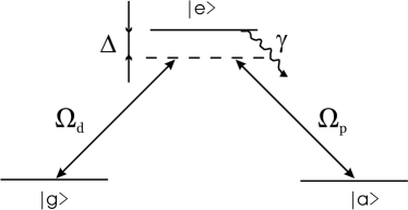
Figure 1: Three-level system coupled by two lasers. $\Omega_{\rm{p}}$ and $\Omega_{\rmd}$ are the Rabi frequencies for the pump and damp laser, $\Delta$ is the one photon detuning, and $\gamma$ is the loss rate.

Note that in this Hamiltonian besides the real-valued one-photon detuning $\Delta$ there is the imaginary term $\gamma$ representing the losses. Denoting the amplitudes of the three-level state as $\psi_{\rme}$, $\psi_{\rm{a}}$, and $\psi_{\rm{g}}$ respectively, we get the Schrödinger equation:

$$\rmi\dot{\psi}_{\rm{a}} = \Omega_{\rm{p}}\psi_{\rme},$$ (2)

$$\rmi\dot{\psi}_{\rme} = -(\Delta+\rmi\gamma)\psi_{\rme}+\Omega_{\rm{p}}\psi_{\rm{a}}+\Omega_{\rm{d}}\psi_{\rm{g}},$$ (3)

$$\rmi\dot{\psi}_{\rm{g}} = \Omega_{\rm{d}}\psi_{\rm{e}}.$$ (4)

The normalization reads:

$$|\psi_{\rm{a}}(t)|^{2}+|\psi_{\rm{g}}(t)|^{2}+|\psi_{\rme}(t)|^{2}\leq 1,$$ (5)

where equality holds for initial time. Because of losses ($\gamma>0$) the total normalization will be slightly reduced (for $t>0$) during the transfer of population through the excited level. This property of the total population is assumed throughout the paper.

We take the laser pulses to be Gaussian

$$\Omega_{\rmd} = \Omega_{0}\exp\left[-\frac{(t-t_{\rmd})^{2}}{T^{2}}\right],$$ (6)

$$\Omega_{\rm{p}} = \Omega_{0}\exp\left[-\frac{(t-t_{\rm{p}})^{2}}{T^{2}}\right].$$ (7)

Here the pulses are centered at $t_{d}$ and $t_{p}$, respectively, $T$ is their width, and $\Omega_{0}$ is their amplitude.

The third order system (2,3,4) may be rewritten in a matrix form

$$\dot{\boldsymbol{\Psi}}=-\rmi H\boldsymbol{\Psi}\equiv A\boldsymbol{\Psi},$$ (8)

where $\boldsymbol{\Psi}=[\psi_{\rm{a}},\psi_{\rme},\psi_{\rm{g}}]^{T}$ is the vector of the state of the system, and

$$H=\left(\begin{array}[]{ccc}0&\Omega_{\rm{p}}&0\\ \Omega_{\rm{p}}&-(\Delta+\rmi\gamma)&\Omega_{\rm{d}}\\ 0&\Omega_{\rm{d}}&0\end{array}\right)$$ (9)

is the corresponding Hamiltonian. The matrix $A\equiv-\rmi H$ is the Jacobian of the system. If the Hamiltonian possesses eigenvalues $\omega$, then the eigenvalues of the Jacobian are defined by $\lambda=-\rmi\omega$. Note that the real parts of $\lambda$ determine the stability of the fixed point at the origin.

We now find these eigenvalues, more specifically their real parts. The eigenvalues of Hamiltonian satisfy the characteristic equation

$$\det||H-I\omega||=0,$$ (10)

with $I$ denoting the unit matrix. Expanding the corresponding third-order determinant one finds that one eigenvalue is always zero:

$$\omega_{1}=0.$$ (11)

The other two eigenvalues satisfy the quadratic equation:

$$\omega^{2}+(\Delta+\rmi\gamma)\omega-(\Omega_{\rm{d}}^{2}+\Omega_{\rm{p}}^{2})=0.$$ (12)

Thus the two eigenvalues satisfy

$$\omega_{2}+\omega_{3} = -[\Delta+\rmi\gamma],$$ (13)

$$\omega_{2}\omega_{3} = -[\Omega_{\rm{d}}^{2}+\Omega_{\rm{p}}^{2}].$$ (14)

Assuming $\Delta=0$, the solutions of (12) read:

$$\omega_{2,3}=\{-\rmi\gamma\pm[-\gamma^{2}+4(\Omega_{\rmd}^{2}+\Omega_{\rm{p}}^{2})]^{1/2}\}/2.$$ (15)

For $t\rightarrow\pm\infty$ the Rabi frequencies go to zero, and it follows from (13,14) that $\omega_{2}=0,\omega_{3}=-\rmi\gamma$. Calling on (11), we can write

$$\lambda_{1,2}=0,\quad\lambda_{3}=-\gamma,$$ (16)

or $\mathrm{Re}(\lambda_{1,2})=0$, and $\mathrm{Re}(\lambda_{3})=-\gamma$ for $t\rightarrow\pm\infty$.

For finite times there is a region where the Rabi frequencies are large enough, so that the discriminant is positive in (15): $D\equiv-\gamma^{2}+4(\Omega_{\rmd}^{2}+\Omega_{\rm{p}}^{2})>0$. Such a situation occurs in a certain interval $t_{1}<t<t_{2}$, and from (15) we get

$$\omega_{2,3} = -\rmi\gamma/2\pm\sqrt{D}/2,$$ (17)

$$\lambda_{2,3} = -\gamma/2\mp\rmi\sqrt{D}/2.$$ (18)

The first eigenvalue is $\lambda_{1}=\omega_{1}=0$. The boundaries $t_{1},t_{2}$ are solutions of $D(t)=0$ in respect to time.

Hence, in the interval $t_{1}<t<t_{2}$, the real parts are $\mathrm{Re}(\lambda_{1})=0$, $\mathrm{Re}(\lambda_{2,3})=-\gamma/2$.

We may adiabatically reduce the dimension of this system but we first transform its variables. We change the bare variables $\psi_{\rm{a}}$, $\psi_{\rm{g}}$ to the bright $\psi_{\rm{B}}$ and dark $\psi_{\rm{D}}$ one:

$$\psi_{\rm{B}} = (\Omega_{\rm{p}}\psi_{\rm{a}}+\Omega_{\rmd}\psi_{\rm{g}})/\Omega,$$ (19)

$$\psi_{\rm{D}} = (\Omega_{\rmd}\psi_{\rm{a}}-\Omega_{\rm{p}}\psi_{\rm{g}})/\Omega,$$ (20)

where

$$\Omega=(\Omega_{\rm{p}}^{2}+\Omega_{\rmd}^{2})^{1/2}.$$ (21)

Denoting $\xi_{\rm{p}}=\Omega_{\rm{p}}/\Omega$, $\xi_{\rmd}=\Omega_{\rmd}/\Omega$, and performing some operations, we obtain the following equations for the new variables:

$$\rmi\dot{\psi}_{\rm{B}} = \alpha\psi_{\rm{D}}+T\Omega\psi_{\rme},$$ (22)

$$\rmi\dot{\psi}_{\rme} = -T(\Delta+\rmi\gamma)\psi_{\rme}+T\Omega\psi_{\rm{B}},$$ (23)

$$\rmi\dot{\psi}_{\rm{D}} = \alpha^{*}\psi_{\rm{B}},$$ (24)

where we have made the time dimensionless by substituting $t/T\rightarrow t$. Here $\alpha=\rmi(\dot{\xi}_{\rm{p}}\xi_{\rmd}-\dot{\xi}_{\rmd}\xi_{\rm{p}})$ is a dimensionless parameter in which derivatives $\dot{\xi}_{\rm{p}},\dot{\xi}_{\rm{d}}$ are taken in respect to dimensionless time.

We now adiabatically eliminate the amplitude $\psi_{\rme}$ by setting $\dot{\psi}_{\rme}=0$. From (23) we get

$$\psi_{\rme}=\frac{\Omega}{\Delta+\rmi\gamma}\psi_{\rm{B}}.$$ (25)

Inserting this result in (22,24) we obtain

$$\rmi\dot{\psi}_{\rm{B}} = \alpha\psi_{\rm{D}}+\frac{T\Omega^{2}}{\Delta+\rmi\gamma}\psi_{\rm{B}},$$ (26)

$$\rmi\dot{\psi}_{\rm{D}} = \alpha^{*}\psi_{\rm{B}}.$$ (27)

We solve this system to find the dynamics of $\psi_{\rm{B}}$, $\psi_{\rm{D}}$, and from (25) we find the dynamics of $\psi_{\rme}$.

The system (26,27) may be also adiabatically reduced. We now set $\dot{\psi}_{\rm{B}}=0$, and solve (26) for $\psi_{\rm{B}}$:

$$\psi_{\rm{B}}=-\frac{\alpha(\Delta+\rmi\gamma)}{T\Omega^{2}}\psi_{\rm{D}}.$$ (28)

Inserting this result in (27), we get a first order dynamic system

$$\rmi\dot{\psi}_{\rm{D}}=-\frac{|\alpha|^{2}(\Delta+\rmi\gamma)}{T\Omega^{2}}\psi_{\rm{D}}.$$ (29)

The Hamiltonian for the $2$D reduced system (26,27) reads:

$$H_{2\rm{D}}=\left(\begin{array}[]{cc}\frac{T\Omega^{2}}{\Delta+\rmi\gamma}&\alpha\\ \alpha^{*}&0\end{array}\right)$$ (30)

Solving the characteristic equation for this Hamiltonian, and assuming $\Delta=0$, one obtains two eigenvalues:

$$\omega_{1,2} = \frac{\rmi}{2}\left[-\frac{T\Omega^{2}}{\gamma}\pm\left(\frac{T^{2}\Omega^{4}}{\gamma^{2}}-4|\alpha|^{2}\right)^{1/2}\right],$$ (31)

$$\lambda_{1,2} = \frac{1}{2}\left[-\frac{T\Omega^{2}}{\gamma}\pm\left(\frac{T^{2}\Omega^{4}}{\gamma^{2}}-4|\alpha|^{2}\right)^{1/2}\right],$$ (32)

Here $\lambda_{1,2}$ are the eigenvalues of the corresponding Jacobian defined as $A_{2\rm{D}}\equiv-\rmi H_{2\rm{D}}$. There are two regimes of evolution of the eigenvalues corresponding to $D_{2}<0$ and $D_{2}>0$, where $D_{2}=\frac{T^{2}\Omega^{4}}{\gamma^{2}}-4|\alpha|^{2}$ is the discriminant in (31,32).

Hence, we have the eigenvalues for all the three versions of the linear lambda system. For the exact $3$D system, they are given by $\lambda_{1}=\omega_{1}=0$ and (17,18). For the reduced $2$D system, they read (31,32). Finally, a trivial single eigenvalue for the $1$D system follows from (29):

$$\lambda_{1}=-\rmi\omega_{1}=-\frac{|\alpha|^{2}\gamma}{T\Omega^{2}}.$$ (33)

In figure 2 we show the dynamics of the real parts of eigenvalues for all three cases.

As the solid lines in figure 2(a) show, for $t<t_{1}$ and $t>t_{2}$ there are two different non-zero branches for the $3$D case: the upper branch determines the slow decay of the bright state, whereas the lower branch causes the fast decay of the excited one. Therefore, we may eliminate the excited state, and cannot do this with the bright one. In the middle of the process, where $t_{1}<t<t_{2}$, both branches become degenerate with real part of eigenvalues equal to $-\gamma/2$. We thus may reduce the both states, excited and bright. During the whole evolution, one real part remains exactly zero showing that the dark state does not experience any losses. This fact indicates that the process is adiabatic.

The short dash dotted and short dash lines show the dynamics of two real parts for the $2$D reduced system. Although the time moments $[(\tilde{t}_{1},\tilde{t}_{2})=(1.24,5.56)]$ at which the discriminant $D_{2}$ is zero differ from the times [$(t_{1},t_{2})=(1.49,5.32)$], where the discriminant $D$ goes to zero, these differences are small compared to the interval $(t_{2}-t_{1})$. In the time intervals of $t<t_{1}$ and $t>t_{2}$ the both branches are close to zero indicating that neither bright nor dark state may be eliminated. The process is here again $2$D. In contrast, in the range of time, where $t_{1}<t<t_{2}$, the decay rate of the bright state is very large compared to that of the dark state. It is well seen in the figure 2(b). Therefore the process is again $1$D as for the exact case.

And lastly, the dotted line shows the dynamics of the real part for the $1$D reduced system. One may clearly see that for $t<t_{1}$ and $t>t_{2}$ the decay of the dark state is rapid compared to that for $t_{1}<t<t_{2}$. The fastness of decay for $t<t_{1}$ and $t>t_{2}$ is seen expressively in the figure 2(b). This leads to conclusion that the $1$D reduced system is appropriate only in the time interval of $t_{1}<t<t_{2}$.

Exactly as for the $3$D system, the evolution of the system in the $2$D ($1$D) approximations is adiabatic for the whole time of integration (in the time interval $t_{1}<t<t_{2}$) since for both cases the decay rate of the dark state is very small compared with that of the bright state.

Figure 2: (a) Dynamics of real parts of eigenvalues of the Jacobian for linear lambda system, computed for all three cases ($3$D, $2$D, and $1$D) by (17,18), (31,32) and (33), respectively. The dashed vertical lines set the boundaries for the $1$D and $2$D processes. Here $t_{1}=1.49$ and $t_{2}=5.32$. The solid lines are the real parts for the $3$D, the short dash dotted and short dash line correspond to the $2$D case, and the dotted line is the real part for the $1$D reduced system; (b) the dynamics of real parts for the $2$D and $1$D cases in extended vertical scale. The lines are chosen in the same way as in (a). The parameters are as follows: $\Delta=0$, $\gamma=2.0$, $\Omega_{0}=10.0$, $t_{\rm{p}}=3.8$, $t_{\rmd}=3.0$, and $T=1.0$.

3 The linear tripod

The STIRAP process in the linear tripod scheme without dissipation was first considered by Unanyan et al. [13, 14]. Here we outline this scheme in which the dissipation is also included. Afterwards we perform the linear analysis of this system.

Consider the four-level system schematically shown in figure 3. The excited state $|\rme\rangle$ is coupled to three ground states $|\rm{a}\rangle$, $|\rm{g1}\rangle$, and $|\rm{g2}\rangle$ with the coupling strengths denoted as $\Omega_{\rm{p}}$, $\Omega_{\rmd 1}$, and $\Omega_{\rmd 2}$, respectively. Here p stands for pump and d stands for the damp. The four-level Hamiltonian reads:

$$\begin{array}[]{l}H=-\hbar(\Delta+\rmi\gamma)|\rme\rangle\langle\rme|+\frac{\hbar}{2}[\Omega_{\rm{p}}|\rm{a}\rangle\langle\rme|+\Omega_{\rmd 1}|\rm{g}1\rangle\langle\rme|+\\ +\Omega_{\rmd 2}|\rm{g}2\rangle\langle\rme|+H.c.].\end{array}$$ (34)

Figure 3: Four-level system coupled by three lasers. $\Omega_{\rm{p}}$ and $\Omega_{\rmd 1}$, $\Omega_{\rmd 2}$ are the Rabi frequencies for the pump, and damp lasers, $\Delta$ is the one photon detuning, and $\gamma$ is the loss rate.

Denoting the amplitudes as $\psi_{\rme}$, $\psi_{\rm{a}}$, $\psi_{\rm{g}1}$, and $\psi_{\rm{g}2}$, the Schrödinger equation reads:

$$\rmi\dot{\psi}_{\rm{a}} = \Omega_{\rm{p}}\psi_{\rme},$$ (35)

$$\rmi\dot{\psi}_{\rme} = -(\Delta+\rmi\gamma)\psi_{\rme}+\Omega_{\rm{p}}\psi_{\rm{a}}+\Omega_{\rmd 1}\psi_{\rm{g}1}+$$ (36)

$$+ \Omega_{\rmd 2}\psi_{\rm{g}2},$$

$$\rmi\dot{\psi}_{\rm{g}1} = \Omega_{\rmd 1}\psi_{\rme},$$ (37)

$$\rmi\dot{\psi}_{\rm{g}2} = \Omega_{\rmd 2}\psi_{\rme}.$$ (38)

The normalization is given by

$$|\psi_{\rm{a}}(t)|^{2}+|\psi_{\rm{g}1}(t)|^{2}+|\psi_{\rm{g}2}(t)|^{2}+|\psi_{\rme}(t)|^{2}\leq 1,$$ (39)

where equality holds for initial time.

The Rabi frequencies are given by

$$\Omega_{\rm{p}} = \Omega_{0}\exp\left[-\frac{(t-t_{\rm{p}})^{2}}{T^{2}}\right],$$ (40)

$$\Omega_{\rmd 1} = K_{1}\Omega_{0}\exp\left[-\frac{(t-t_{\rmd 1})^{2}}{T^{2}}\right],$$ (41)

$$\Omega_{\rmd 2} = K_{2}\Omega_{0}\exp\left[-\frac{(t-t_{\rmd 2})^{2}}{T^{2}}\right].$$ (42)

Here the pulses are centered at $t_{\rm{p}}$, $t_{\rmd 1}$ and $t_{\rmd 2}$, respectively. $T$ is the width of the pulses, $K_{1}$, $K_{2}$ determine the amplitudes for the damp pulses, and $\Omega_{0}$ is the amplitude for the pump pulse.

The system (35,36,37,38) can be written in the form of (8) with the state vector $\boldsymbol{\Psi}=[\psi_{\rm{a}},\psi_{\rme},\psi_{\rm{g}1},\psi_{\rm{g}2}]^{T}$, and Hamiltonian

$$H=\left(\begin{array}[]{cccc}0&\Omega_{\rm{p}}&0&0\\ \Omega_{\rm{p}}&-(\Delta+\rmi\gamma)&\Omega_{\rmd 1}&\Omega_{\rmd 2}\\ 0&\Omega_{\rmd 1}&0&0\\ 0&\Omega_{\rmd 2}&0&0\end{array}\right)$$ (43)

The matrix $A\equiv-\rmi H$ is again the Jacobian of the system. Here the relation $\lambda=-\rmi\omega$ holds. Solving the eigenvalues problem (10) for the linear tripod, we obtain two zero eigenvalues,

$$\omega_{1,2}=0.$$ (44)

The other two eigenvalues can be found from quadratic equation

$$\omega^{2}+(\Delta+\rmi\gamma)\omega-(\Omega_{\rmd 1}^{2}+\Omega_{\rmd 2}^{2}+\Omega_{\rm{p}}^{2})=0.$$ (45)

The eigenvalues $\omega_{3,4}$ must satisfy

$$\omega_{3}+\omega_{4} = -(\Delta+\rmi\gamma),$$ (46)

$$\omega_{3}\omega_{4} = -(\Omega_{\rmd 1}^{2}+\Omega_{\rmd 2}^{2}+\Omega_{\rm{p}}^{2}).$$ (47)

We again assume that $\Delta=0$, thus obtaining the following solutions:

$$\omega_{3,4}=\{-\rmi\gamma\pm[-\gamma^{2}+4(\Omega_{\rmd 1}^{2}+\Omega_{\rmd 2}^{2}+\Omega_{\rm{p}}^{2})]^{1/2}\}/2.$$ (48)

(See also (7) in [14]). The Rabi frequencies are chosen in the form of Gaussian pulses. For $t\rightarrow\pm\infty$ the Rabi frequencies tend to zero, and from (46,47) it follows that $\omega_{3}=0$, $\omega_{4}=-\rmi\gamma$. Hence, for $t\rightarrow\pm\infty$ we have

$$\lambda_{1,2,3}=0,\quad\lambda_{4}=-\gamma.$$ (49)

However between these two infinite times there is a region where the Rabi frequencies are large enough, and the discriminant in (48) is positive $[D\equiv-\gamma^{2}+4(\Omega_{\rmd 1}^{2}+\Omega_{\rmd 2}^{2}+\Omega_{\rm{p}}^{2})>0]$. Such a situation takes place in the interval $t_{1}<t<t_{2}$, and from (48) we get

$$\omega_{3,4} = -\rmi\gamma/2\pm\sqrt{D}/2,$$ (50)

$$\lambda_{3,4} = -\gamma/2\mp\rmi\sqrt{D}/2.$$ (51)

The first two eigenvalues are $\lambda_{1,2}=\omega_{1,2}=0$. The boundaries $t_{1},t_{2}$ are defined in the same way as in section 3.

Hence, in the interval $t_{1}<t<t_{2}$, the real parts are $\mathrm{Re}(\lambda_{1,2})=0$, $\mathrm{Re}(\lambda_{3,4})=-\gamma/2$.

Exactly as in the previous section, we first transform the variables from the bare states to one bright and two dark states:

$$(\psi_{\rm{a}},\psi_{\rme},\psi_{\rm{g}1},\psi_{\rm{g}2})\rightarrow(\psi_{\rm{B}},\psi_{\rme},\psi_{\rm{D}1},\psi_{\rm{D}2}).$$ (52)

Parametrizing the Rabi frequencies as

$$\Omega_{\rmd 2} = \Omega\sin{(\phi)},$$ (53)

$$\Omega_{\rm{p}} = \Omega\cos{(\phi)}\sin{(\Theta)},$$ (54)

$$\Omega_{\rmd 1} = \Omega\cos{(\phi)}\cos{(\Theta)},$$ (55)

we may write down the amplitudes of one bright and two dark states:

$$\psi_{\rm{B}} = \cos{(\phi)}\sin{(\Theta)}\psi_{\rm{a}}+\cos{(\phi)}\cos{(\Theta)}\psi_{\rm{g}1}+$$ (56)

$$+ \sin{(\phi)}\psi_{\rm{g}2},$$

$$\psi_{\rm{D}1} = \cos{(\Theta)}\psi_{\rm{a}}-\sin{(\Theta)}\psi_{\rm{g}1},$$ (57)

$$\psi_{\rm{D}2} = \sin{(\phi)}\sin{(\Theta)}\psi_{\rm{a}}+\sin{(\phi)}\cos{(\Theta)}\psi_{\rm{g}1}-$$ (58)

$$- \cos{(\phi)}\psi_{\rm{g}2}.$$

After renormalizing the time ($t/T\rightarrow t$) and some rearrangements, we derive the following dynamic system for these variables:

$$\rmi\frac{\rmd}{\rmd t}\left(\begin{array}[]{c}\psi_{\rm{B}}\\ \psi_{\rme}\\ \psi_{\rm{D}1}\\ \psi_{\rm{D}2}\end{array}\right)=\left(\begin{array}[]{cccc}0&T\Omega&\alpha_{13}&\alpha_{14}\\ T\Omega&-T(\Delta+\rmi\gamma)&0&0\\ \alpha^{*}_{13}&0&0&\alpha_{34}\\ \alpha^{*}_{14}&0&\alpha^{*}_{34}&0\end{array}\right)\left(\begin{array}[]{c}\psi_{\rm{B}}\\ \psi_{\rme}\\ \psi_{\rm{D}1}\\ \psi_{\rm{D}2}\end{array}\right).$$ (59)

Here

$$\alpha_{13} = \rmi(\dot{\xi}_{11}\xi_{31}+\dot{\xi}_{13}\xi_{33}),$$ (60)

$$\alpha_{14} = \rmi(\dot{\xi}_{11}\xi_{41}+\dot{\xi}_{13}\xi_{43}+\dot{\xi}_{14}\xi_{44}),$$ (61)

$$\alpha_{34} = \rmi(\dot{\xi}_{31}\xi_{41}+\dot{\xi}_{33}\xi_{43}),$$ (62)

and the coefficients $\xi_{ij}$ are defined by the matrix

$$||\xi_{ij}||=\left(\begin{array}[]{cccc}\cos{(\phi)}\sin{(\Theta)}&0&\cos{(\phi)}\cos{(\Theta)}&\sin{(\phi)}\\ 0&1&0&0\\ \cos{(\Theta)}&0&-\sin{(\Theta)}&0\\ \sin{(\phi)}\sin{(\Theta)}&0&\sin{(\phi)}\cos{(\Theta)}&-\cos{(\phi)}\end{array}\right).$$ (63)

Note that this matrix realizes the transformation (52) (see also (56,57,58)).

We now reduce the dimension of system (59) in two steps. For the first step, we eliminate the excited state by setting

$$\dot{\psi}_{\rme}=0.$$ (64)

Solving the equation

$$\Omega\psi_{\rm{B}}-(\Delta+\rmi\gamma)\psi_{\rme}=0,$$ (65)

(see the second row in (59)) for $\psi_{\rme}$, we get

$$\psi_{\rme}=\frac{\Omega}{\Delta+\rmi\gamma}\psi_{\rm{B}}.$$ (66)

Inserting this result in (59), we obtain the following three-dimensional dynamic system:

$$\rmi\frac{\rmd}{\rmd t}\left(\begin{array}[]{c}\psi_{\rm{B}}\\ \psi_{\rm{D}1}\\ \psi_{\rm{D}2}\end{array}\right)=\left(\begin{array}[]{ccc}\frac{T\Omega^{2}}{\Delta+\rmi\gamma}&\alpha_{13}&\alpha_{14}\\ \alpha^{*}_{13}&0&\alpha_{34}\\ \alpha^{*}_{14}&\alpha^{*}_{34}&0\end{array}\right)\left(\begin{array}[]{c}\psi_{\rm{B}}\\ \psi_{\rm{D}1}\\ \psi_{\rm{D}2}\end{array}\right).$$ (67)

We can solve this system to find the evolution of $\psi_{\rm{B}}$, $\psi_{\rm{D}1}$, $\psi_{\rm{D}2}$, and to determine the dynamics of the excited state using (66).

For the second step, we eliminate the bright state, i.e. we set

$$\dot{\psi}_{\rm{B}}=0,$$ (68)

in (67). After solving the equation

$$\frac{T\Omega^{2}}{\Delta+\rmi\gamma}\psi_{\rm{B}}+\alpha_{13}\psi_{\rm{D}1}+\alpha_{14}\psi_{\rm{D}2}=0$$ (69)

for $\psi_{\rm{B}}$ (see the first row in (67)), we find

$$\psi_{\rm{B}}=-\frac{\Delta+\rmi\gamma}{T\Omega^{2}}(\alpha_{13}\psi_{\rm{D}1}+\alpha_{14}\psi_{\rm{D}2}).$$ (70)

Inserting this result in (67), we obtain the following second order system:

$$\rmi\frac{\rmd}{\rmd t}\left(\begin{array}[]{c}\psi_{\rm{D}1}\\ \psi_{\rm{D}2}\end{array}\right)=H_{2}\left(\begin{array}[]{c}\psi_{\rm{D}1}\\ \psi_{\rm{D}2}\end{array}\right).$$ (71)

The matrix of this system may be split into two parts:

$$H_{2}=H^{(0)}_{2}+\frac{\Delta+\rmi\gamma}{T\Omega^{2}}H^{(1)}_{2},$$ (72)

where

$$H^{(0)}_{2}=\left(\begin{array}[]{cc}0&\alpha_{34}\\ \alpha^{*}_{34}&0\end{array}\right),$$ (73)

and

$$H^{(1)}_{2}=-\left(\begin{array}[]{cc}|\alpha_{13}|^{2}&\alpha^{*}_{13}\alpha_{14}\\ \alpha^{*}_{14}\alpha_{13}&|\alpha_{14}|^{2}\end{array}\right).$$ (74)

When $\Omega^{2}$ is relatively large, one can neglect the influence of $H^{(1)}_{2}$ and write approximately $H_{2}\simeq H^{(0)}_{2}$. Thus one arrives at a simple second order system

$$\rmi\frac{\rmd}{\rmd t}\left(\begin{array}[]{c}\psi_{\rm{D}1}\\ \psi_{\rm{D}2}\end{array}\right)=\left(\begin{array}[]{cc}0&\alpha_{34}\\ \alpha^{*}_{34}&0\end{array}\right)\left(\begin{array}[]{c}\psi_{\rm{D}1}\\ \psi_{\rm{D}2}\end{array}\right),$$ (75)

which is equivalent to (27) of [13]. However, this system is not an adiabatically reduced version of the system (35,36,37,38). Actually, it determines the solution moving exactly on the dark state manifold comprising the two degenerate states $|D1\rangle$ and $|D2\rangle$ (this statement can be confirmed by applying the approach of [32]). Comparing (72) with the corresponding result for the linear lambda system, (29), we note that the both Hamiltonians contain the characteristic time scale $T$ (the pulse width) in the denominators. In the case of (72) this time scale is involved only with the correction Hamiltonian $H^{(1)}_{2}$, and it is absent in $H^{(0)}_{2}$ since it corresponds to a zero on the r.h.s. of (29). The correction $H^{(1)}_{2}$ in (72) thus corresponds to the r.h.s. of (29).

Figure 4 shows the dynamics of the real parts of the eigenvalues of the Jacobians for various dimensions. In figure 4(a) the solid lines correspond to the exact $4$D case. For $t<t_{1}$ and $t>t_{2}$ the lower branch, for which $\mathrm{Re}\lambda\simeq-\gamma$, causes the decay of the excited state. The upper branch describing the decay rate for the bright state is small compared to the decay rate of the excited state in these time intervals indicating that the excited state may be adiabatically eliminated, whereas the bright state must be left. In the middle of the passage ($t_{1}<t<t_{2}$) the decay rates of the excited and bright states become degenerate and equal to $-\gamma/2$, thus enabling to eliminate them both. The eigenvalues for the dark states remain both zeros for the whole evolution of the system demonstrating that the process is adiabatic since the degenerate dark state does not loose its population.

The dash dotted line in figure 4 displays the dynamics of the decay rate for the bright state in the $3$D system. In figure 4(a) it falls down (grows up) just after $t_{1}$ (just before $t_{2}$). In figure 4(b) the same dynamics is shown in extended vertical scale. From both figures, 4(a) and 4(b), one may conclude that in the $3$D reduced system the bright state may be eliminated for $t_{1}<t<t_{2}$, and it should be preserved for $t<t_{1}$ and $t>t_{2}$, since its decay rate in the latter case is much less than in the former one. The two eigenvalues corresponding to degenerate dark states remain exactly (or almost) zero for the $3$D system. They are small compared with the decay rate of the bright state. Therefore these states may not be eliminated for the whole time of evolution.

The dotted and short dotted lines in figure 4 show the dynamics of the real parts for the $2$D reduced system. One of them grows rapidly before $t_{1}$ and converges to zero, whereas the other one is first zero and then decays rapidly after $t_{2}$. Such a situation suggests that the range of applicability of the $2$D system should be wider than the time interval $t_{1}<t<t_{2}$ since the two degenerate dark states survive (do not decay) when the decay rate is relatively small. However, such a conclusion would be true if we distributed the whole population among the degenerate states at the end of the rapid growth of the first real part. But if the bright state had some initial population, it could not be neglected since its real part is close to zero before $t_{1}$ and after $t_{2}$.

We should also note here that for the $2$D reduced system, the decay rate for the second dark state grows rapidly from negative values to zero (the decay rate for the first dark state decreases rapidly from zero to negative values) in the time intervals $t<2.0$ ($t>18.0$), i.e. outside of the figure 4. But we do not need to take these events into account since we are interested in the time interval where both decay rates are close to zero. This interval is determined by the growing (decreasing) decay rates which are plotted in the figure 4.

Exactly as in the previous section, we here can also conclude that the adiabaticity is preserved also for reduced systems, since for the $3$D ($2$D) approximations the dark states manifold does not loose its population for the whole time of evolution (in the time interval that is wider than $t_{1}<t<t_{2}$).

Figure 4: (a) Dynamics of real parts of eigenvalues of the Jacobian for linear tripod, computed for all three cases ($4$D, $3$D and $2$D) by [(48),(44)], from (67) and (72), respectively. The dashed vertical lines set the boundaries for the $2$D and $3$D processes. Here $t_{1}=6.12$ and $t_{2}=12.73$. The solid lines are the real parts for the $4$D, the short dash dotted and short dash line correspond to $3$D case, and the dotted and the short dotted lines are the real parts for the $2$D reduced system; (b) the dynamics of real parts for the $3$D and $2$D cases in extended vertical scale. The lines are chosen in the same way as in (a). The parameters are as follows: $\Delta=0$, $\gamma=2.0$, $\Omega_{0}=60.0$, $t_{\rm{p}}=10.7$, $t_{\rmd 1}=10.0$, $t_{\rmd 2}=8.5$, $K_{1}=0.75$, $K_{2}=5.0$, and $T=1.0$.

Figure 5 displays the results of numerical computations. In figure 5(a) we have presented the dynamics of populations of the bright (dashed and dotted lines), and excited (dashed-dotted and short-dotted lines) states. The dashed and dotted lines correspond to solutions of exact equations (35,36,37,38). The dashed-dotted and short-dotted lines are obtained from (67) (the bright state), and from (66) (the excited state). One can see that the populations of these states remain relatively small ($P_{\rme},P_{\rm{B}}\simeq 10^{-3}$). In figure 5(b) the dynamics of coupling strengths is shown. Figures 5(c,d) display the dynamics of populations of the degenerate dark states. Figure 5(c) presents the solutions of exact (35,36,37,38) (thin solis line) and that of adiabatically reduced system (67) (thick solid line). The exact and approximate solutions are in good quantitative agreement (we do not distinguish them in the present graph). Both systems were integrated in the whole time range ($t\in[0.0,20.0]$). In figure 5(d) we compare the dynamics for exact (35,36,37,38) (thin solid line) with those of adiabatically simplified (71) (thick solid line).

Figure 5: (a) The dynamics of populations $10^{3}P_{\rme},10^{3}P_{\rm{B}}$ that are computed from (35,36,37,38) (dashed/dash-dotted lines), and from (67), (66) (dotted/short-dotted lines); (b) the dynamics of Gaussian pulses computed by (40,41,42); (c,d) the dynamics of populations of dark states computed in (c) by (35,36,37,38) (thin solid line), and by (67) (thick solid line); in (d) the thin solid line represents again the exact solution of (35,36,37,38), and thick solid line is obtained using the approximation from (71) computed in the range of $t_{1}<t<t_{2}$. The parameters are the same as in figure 4. The initial conditions are $\psi_{\rm{a}}(0)=1$, $\psi_{\rm{g}1}(0)=\psi_{\rm{g}2}(0)=\psi_{\rme}(0)=0$.

In figure 6 we compare the exactness of various approximations for the non-linear tripod. We see that the system (75) is in a good quantitative agreement with the exact system, but it is worse than (67) in the range $t>t_{1}$. Whereas the $2$D approximation (71) coincides with the solution of (67) in the interval $t_{1}<t<t_{2}$ almost identically. At the end of this interval, just before $t_{2}$, the solution of (71) slightly deviates from that of (67). This is due to the fact that the magnitude of element $\frac{\gamma}{T\Omega^{2}}|\alpha_{13}|^{2}$ contributed by the matrix $H^{(1)}_{2}$ in (72) becomes large compared with the magnitude of the element $\alpha_{34}$ of the matrix $H^{(0)}_{2}$, (73). The remaining elements of $H^{(1)}_{2}$ are much less than $|\alpha_{13}|^{2}$ just before $t_{2}$.

We should also note that in figure 6 the solution of ”non-exact” $2$D system (73) coincides almost identically with the exact $4$D solution in the range of $t<t_{1}$. However, such a situation takes place when the initial conditions are very close to the dark state. If we pushed them away from the dark state, the result of (73) would become worse than that of the $3$D system (67) (not shown here). The system thus remains effectively $3$D in the range of $t<t_{1}$.

Similarly it can be numerically verified that the solution of (71) is not worse than that of (67) just before $t_{2}$ if one pushes the initial conditions further away from the dark state manifold. Therefore the system remains $2$D in the whole interval $t_{1}<t<t_{2}$.

Figure 6: The differences between the exact and approximated degenerate dark states; the short dotted and dotted lines show the differences of $P_{\rm{D}1}-P^{\rm{ad}}_{\rm{D}1}$ and $P_{\rm{D}2}-P^{\rm{ad}}_{\rm{D}2}$ for the $3$D system (67), respectively; the dash dotted and short dash dotted lines display the corresponding differences for $P_{\rm{D}1}$ and $P_{\rm{D}2}$ for the $2$D system (75), respectively; the solid and dashed lines show the differences for $P_{\rm{D}1}$ and $P_{\rm{D}2}$ for the adiabatically reduced system (71), respectively (integrated only in the range of $t_{1}<t<t_{2}$). The vertical dashed lines set the boundaries for the $3$D and $2$D processes. The parameters and initial conditions are the same as in figure 5.

4 The non-linear lambda system

The three-level non-linear Hamiltonian for the non-linear lambda system (see the figure 1) reads:

$$\begin{array}[]{l}\hat{H}=-\hbar(\Delta+\rmi\gamma)\hat{\psi}_{\rme}^{{\dagger}}\hat{\psi}_{\rme}+\frac{\hbar}{2}(\Omega_{\rm{p}}\hat{\psi}_{\rme}^{{\dagger}}\hat{\psi}_{\rm{a}}\hat{\psi}_{\rm{a}}+\Omega_{\rmd}\hat{\psi}_{\rme}^{{\dagger}}\hat{\psi}_{\rm{g}}\\ +H.c.).\end{array}$$ (76)

Here $\hat{\psi}_{\alpha},\hat{\psi}^{{\dagger}}_{\alpha}$ ($\alpha=\rm{a},\rme,\rm{g}$) are the bosonic annihilation and creation operators for state $\alpha$, respectively. When the number of particles is much larger than the unity, the boson operators are replaced by $c$ numbers $\psi_{\alpha},\psi^{*}_{\alpha}$ (the meanfield treatment [29, 37]) which obey the following Heisenberg equations

$$\rmi\dot{\psi}_{\rm{a}} = \Omega_{\rm{p}}\psi_{\rm{a}}^{*}\psi_{\rme},$$ (77)

$$\rmi\dot{\psi}_{\rme} = -(\Delta+\rmi\gamma)\psi_{\rme}+\frac{1}{2}\Omega_{\rm{p}}\psi_{\rm{a}}^{2}+\frac{1}{2}\Omega_{\rmd}\psi_{\rm{g}},$$ (78)

$$\rmi\dot{\psi}_{\rm{g}} = \frac{1}{2}\Omega_{\rmd}\psi_{\rme}.$$ (79)

The normalization reads:

$$|\psi_{\rm{a}}(t)|^{2}+2[|\psi_{\rm{g}}(t)|^{2}+|\psi_{\rme}(t)|^{2}]\leq 1,$$ (80)

where the equality holds for the initial time.

The nonlinearity enters here in the coupling induced by the pump field: it couples a particle in the state $e$ with a pair of particles in the state $a$. Such a nonlinear couplig is encountered in second harmonic generation in nonlinear optics (where $a$ represents the fundamental photon and $e$ its second harmonics), as well as in the photoassociation of atoms into diatomic molecules [20, 21, 29, 37], where $a$ represents an atomic state, while $e$ and $g$ are excited and ground diatomic molecular states, respectively.

As for the linear lambda system, we take the Gaussian pulses given by (6,7).

Similarly as in two previous sections, we here define the state vector $\boldsymbol{\Psi}=[\psi_{\rm{a}},\psi_{\rme},\psi_{\rm{g}}]^{T}$. The dynamic system (77,78,79) can be rewritten in the vector form:

$$\rmi\frac{\rmd}{\rmd t}\boldsymbol{\Psi}=\bi{f}(\boldsymbol{\Psi}),$$ (81)

where $\bi{f}$ is the vector of (generally) non-linear functions on the r.h.s. of system (77,78,79). The steady state solution $\boldsymbol{\Psi}_{0}(t)$ of this system represents the dark state which is obtained by solving

$$\bi{f}(\boldsymbol{\Psi}_{0})=\mathbf{0}.$$ (82)

For the non-linear lambda system (77,78,79) the dark state reads ([29, 37]):

$$\psi^{0}_{\rm{a}}=\left[\frac{2\Omega_{\rmd}}{\Omega_{\rmd}+\Omega_{\rm{eff}}}\right]^{1/2},\quad\psi^{0}_{\rme}=0,\quad\psi^{0}_{\rm{g}}=-\frac{2\Omega_{\rm{p}}}{\Omega_{\rmd}+\Omega_{\rm{eff}}},$$ (83)

with $\Omega_{\rm{eff}}=(\Omega^{2}_{\rmd}+8\Omega^{2}_{\rm{p}})^{1/2}$.

If the solution remains in this state for the whole time, the adiabatic passage from initially occupied state $a$ to the target state $g$ takes place provided the Gaussian pulses $\Omega_{\rmd}(t)$, $\Omega_{\rm{p}}(t)$ arrive in a counter-intuitive sequence.

We are now interested in the linear stability of the dark state (83). To this end, we suppose that the solution of (81) evolves in the close neighbourhood of the dark state $\boldsymbol{\Psi}_{0}$, i.e. we express it as a sum

$$\boldsymbol{\Psi}(t)=\boldsymbol{\Psi}_{0}(t)+\delta\boldsymbol{\Psi}(t),$$ (84)

where $\delta\boldsymbol{\Psi}(t)$ is a deviation of the current solution from the dark state. Inserting this expression in (81) yields

$$\rmi\dot{\boldsymbol{\Psi}}_{0}(t)+\rmi\frac{\rmd}{\rmd t}\delta\boldsymbol{\Psi}(t)=\bi{f}(\boldsymbol{\Psi}_{0}(t)+\delta\boldsymbol{\Psi}(t)).$$ (85)

Using (82), one finds

$$\rmi\frac{\rmd}{\rmd t}\delta\boldsymbol{\Psi}=M\delta\boldsymbol{\Psi}-\rmi\dot{\boldsymbol{\Psi}}_{0}.$$ (86)

where $M$ is a matrix with the elements $M_{ij}=\frac{\partial f_{i}}{\partial\psi_{j}}$ with $i,j=\rm{a},\rme,\rm{g}$. Here the partial derivatives are calculated at the dark state. In system (86) the non-linear terms have been omitted.

Specifically, for the system (77,78,79), the matrix $M$ reads

$$M=\left(\begin{array}[]{ccc}0&\Omega_{\rm{p}}\psi^{0*}_{\rm{a}}&0\\ \Omega_{\rm{p}}\psi^{0}_{\rm{a}}&-(\Delta+\rmi\gamma)&\Omega_{\rmd}/2\\ 0&\Omega_{\rmd}/2&0\end{array}\right).$$ (87)

(See also (7) in [23]). It is similar to the Hamiltonian (9) of the linear lambda system. The difference is that the elements $M_{\rm{ae}}$ and $M_{\rm{ea}}$ contain the component of the dark state $\psi^{0}_{\rm{a}}$ due to the nonlinearity.

Denoting the Jacobian as $A=-\rmi M$, we can rewrite the linearised equation (86) as

$$\frac{\rmd}{\rmd t}\delta\boldsymbol{\Psi}=A\delta\boldsymbol{\Psi}-\dot{\boldsymbol{\Psi}}_{0}.$$ (88)

In this system, the real parts of the eigenvalues of the Jacobian $A$ determine the stability of the dark state. If the matrix $M$ has eigenvalues $\omega$, the Jacobian $A$ has the eigenvalues $\lambda=-\rmi\omega$. In analogy to the linear lambda system, the eigenvalues $\omega$ can be found from the characteristic equation

$$\det||M-I\omega||=0.$$ (89)

Solving (89) with (87), we find that one root is always zero:

$$\omega_{1}=0.$$ (90)

The other two eigenvalues obey the quadratic equation:

$$\omega^{2}+(\Delta+\rmi\gamma)\omega-(\Omega_{\rmd}^{2}+4\Omega_{\rm{p}}^{2}|\psi^{0}_{\rm{a}}|^{2})/4=0.$$ (91)

The corresponding eigenvalues $\omega_{2}$ and $\omega_{3}$ obey the following

$$\omega_{2}+\omega_{3} = -(\Delta+\rmi\gamma),$$ (92)

$$\omega_{2}\omega_{3} = -(\Omega_{\rmd}^{2}+4\Omega_{\rm{p}}^{2}|\psi^{0}_{\rm{a}}|^{2})/4.$$ (93)

By setting $\Delta=0$, we get the solutions of quadratic equation:

$$\omega_{2,3}=[-\rmi\gamma\pm(-\gamma^{2}+\Omega_{\rmd}^{2}+4\Omega_{\rm{p}}^{2}|\psi^{0}_{\rm{a}}|^{2})^{1/2}]/2.$$ (94)

(See also the equations under (7) in [23]).

In figure 7 we show the dynamics of $\mathrm{Re}(\lambda(t))$ for the non-linear lambda system. One can see that this picture reproduces the same behaviour as the corresponding dependence for the linear lambda system shown in figure 2. This means that the real parts of eigenvalues of the Jacobian for the nonlinear lambda system are the same as those for the linear system in the corresponding time intervals: $t<t_{1}$, $t>t_{2}$ and $t_{1}<t<t_{2}$.

We now adiabatically eliminate the excited state by setting $\dot{\psi}_{\rme}=0$. From (78) we get

$$\psi_{\rme}=\frac{1}{2(\Delta+\rmi\gamma)}(\Omega_{\rm{p}}\psi^{2}_{\rm{a}}+\Omega_{\rmd}\psi_{\rm{g}}).$$ (95)

Inserting this result into (77,79) we obtain a second order system

$$\rmi\dot{\psi}_{\rm{a}} = \Omega_{\rm{p}}\psi_{\rm{a}}^{*}\psi_{\rme},$$ (96)

$$\rmi\dot{\psi}_{\rm{g}} = \frac{1}{2}\Omega_{\rmd}\psi_{\rme}.$$ (97)

with $\psi_{\rme}$ given by (95).

We now discuss the validity of $3$D and $2$D systems. The $3$D system (77,78,79) is valid for all times. In the ranges $t<t_{1}$ and $t>t_{2}$ the $2$D system (96,97) can be applied since there are two zero real parts $\mathrm{Re}(\lambda_{1,2})=0$, and one negative real part $\mathrm{Re}(\lambda_{3})\simeq-\gamma$. In the range $t_{1}<t<t_{2}$ the process is $1$D since there is only one zero real part $\mathrm{Re}(\lambda_{1})=0$ and two negative real parts $\mathrm{Re}(\lambda_{2,3})=-\gamma/2$. However, here we do not have any $1$D equation, one can only propose the $2$D system (96,97). The search for a $1$D system is a challenging problem.

Figure 7: Dynamics of real parts of eigenvalues of the Jacobian for non-linear lambda system, computed by (94), and (90). The dashed vertical lines set the boundaries for the $1$D and $2$D processes. Here $t_{1}=0.76$ and $t_{2}=5.71$. The parameters are as follows: $\Delta=0$, $\gamma=2.0$, $\Omega_{0}=300.0$, $t_{\rm{p}}=3.8$, and $t_{\rmd}=3.0$.

In the figure 8 we have plotted the relevant dynamics for the case of adiabatically reduced non-linear lambda system. In the figure 8(a) we show the Gaussian pulses that are ordered counter-intuitively. From figure 8(b) one may conclude that the solutions of adiabatically reduced system are in good quantitative agreement with the solutions of exact system (we do not distinguish them in the figure). In figure 8(c) we see that the difference for $P_{\rme}$ between exact and approximated solutions is significant. It can be explained by the fact that the magnitude of probability $P_{\rme}$ is small. On the other hand, the difference in the case of $P_{\rm{a}}$, $P_{\rm{g}}$ is of the same order but we do not distinguish it, since the magnitudes of these quantities are much larger. In figure 8(d) we have plotted the dynamics of the difference between the exact ($P_{\rm{a}}$) and adiabatically reduced ($P^{\rm{ad}}_{\rm{a}}$) solutions of the population $P_{\rm{a}}$. (See also the blue line in figure 2(c) in [25]). The difference is of the same order as that in figure 8(c).

Figure 8: The dynamics (a) of Gaussian pulses (6,7), (b) of populations $P_{\rm{a}}$, $P_{\rm{g}}$, (c) of population $P_{\rme}$ in enlarged scale, and (d) the difference of $P_{\rm{a}}$ between exactly ($P_{\rm{a}}$) and adiabatically ($P^{\rm{ad}}_{\rm{a}}$) obtained solutions. In (b,c) the solid thin lines represent the solutions of exact (77,78,79), and the (solid thick/dotted) lines are the solutions of adiabatically reduced system (96,97) with excited state given by (95). The parameters are the same as in figure 7. The initial conditions are $\psi_{\rm{a}}(0)=1$, $\psi_{\rm{g}}(0)=\psi_{\rme}(0)=0$.

In figure 9 we have plotted the dynamics of differences between the populations of the current state and corresponding dark state. The difference for the initial ground state $a$ deviates up to $0.03$ at the end of the passage. Whereas the difference for the excited state remains much less. The corresponding difference for state $g$ is almost symmetric to that of the state $a$ in respect to the zero (not shown here). We conclude that the process is adiabatic since the solution remains in a close neighborhood to the dark state.

Figure 9: The dynamics of the differences of populations between the current state and the dark state, for $\delta P_{\rm{a}}(t)=|\psi_{\rm{a}}(t)|^{2}-|\psi^{0}_{\rm{a}}(t)|^{2}$ (solid line), and $\delta P_{\rme}(t)=2|\psi_{\rme}(t)|^{2}$ (dashed line) for the nonlinear lambda system. The dynamics of $\psi_{\rm{a}}(t),\psi_{\rme}(t)$ are computed from (77,78,79), and $\psi^{0}_{\rm{a}}(t)$ is given by (83). The parameters are the same as in figure 7. The initial conditions are $\psi_{\rm{a}}(0)=1$, $\psi_{\rm{g}}(0)=\psi_{\rme}(0)=0$.

5 The non-linear tripod

We consider the atom-molecule transition in ultracold quantum gases via photoassociation. This problem has potential applications during the creation of ultracold molecules and quantum superchemistry. The underlying physics is closely related to the STIRAP and has been widely studied in the context of atomic physics and quantum optics [52, 3].

The level structure of the atom-molecule tripod system is shown in figure 3. In ultracold atomic systems, the level $a$ denotes the atomic Bose-Einstein condensation (BEC), which couples an excited state of a diatomic molecular BEC via the pump field $\Omega_{\rm{p}}(t)$. Such an excited state is represented by high-lying vibration levels of the single excited molecule. The excited state is coupled to the two ground states of the molecular BEC, $g1$ and $g2$, with the strengths $\Omega_{\rmd 1}(t)$ and $\Omega_{\rmd 2}(t)$, respectively.

Assuming a two-photon resonance condition, the four-level non-linear Hamiltonian for non-linear tripod takes the form:

$$\begin{array}[]{l}\hat{H}=-\hbar(\Delta+\rmi\gamma)\hat{\psi}_{\rme}^{{\dagger}}\hat{\psi}_{\rme}+\frac{\hbar}{2}(\Omega_{\rm{p}}\hat{\psi}_{\rme}^{{\dagger}}\hat{\psi}_{\rm{a}}\hat{\psi}_{\rm{a}}+\Omega_{\rmd 1}\hat{\psi}_{\rme}^{{\dagger}}\hat{\psi}_{\rm{g}1}+\\ \Omega_{\rmd 2}\hat{\psi}_{\rme}^{{\dagger}}\hat{\psi}_{\rm{g}2}+H.c.).\end{array}$$ (98)

Here $\hat{\psi}_{\alpha},\hat{\psi}^{{\dagger}}_{\alpha}$ ($\alpha=\rm{a},\rme,\rm{g}1,\rm{g}2$) are the bosonic annihilation and creation operators for state $\alpha$, respectively. To explore the behaviour of the system under time evolution, we consider the problem under mean-field approximation, which is reasonable for bosonic systems when the number of particles is large compared with unity [29, 37]. In this limit, the bosonic operators are replaced by $c$ numbers, and the Heisenberg equation leads to the following equations of motion for the probability amplitudes:

$$\rmi\dot{\psi}_{\rm{a}} = \Omega_{\rm{p}}\psi_{\rm{a}}^{*}\psi_{\rme},$$ (99)

$$\rmi\dot{\psi}_{\rme} = -(\Delta+\rmi\gamma)\psi_{\rme}+\frac{1}{2}\Omega_{\rm{p}}\psi_{\rm{a}}^{2}+\frac{1}{2}\Omega_{\rmd 1}\psi_{\rm{g}1}+$$ (100)

$$+ \frac{1}{2}\Omega_{\rmd 2}\psi_{\rm{g}2},$$

$$\rmi\dot{\psi}_{\rm{g}1} = \frac{1}{2}\Omega_{\rmd 1}\psi_{\rme},$$ (101)

$$\rmi\dot{\psi}_{\rm{g}2} = \frac{1}{2}\Omega_{\rmd 2}\psi_{\rme}.$$ (102)

The nonlinear term enters here when the molecules are obtained via associating cold atoms.

The normalization reads:

$$|\psi_{\rm{a}}(t)|^{2}+2[|\psi_{\rm{g}1}(t)|^{2}+|\psi_{\rm{g}2}(t)|^{2}+|\psi_{\rme}(t)|^{2}]\leq 1,$$ (103)

where the equality holds for the initial time.

Like in the case of linear tripod, the Gaussian pulses are given by (40,41,42).

Similar to the linear case, we define the following state vector of the system: $\boldsymbol{\Psi}=[\psi_{\rm{a}},\psi_{\rme},\psi_{\rm{g}1},\psi_{\rm{g}2}]^{T}$. The dynamic equations (99,100,101,102) can be rewritten in a vector form given by (81), where $\bi{f}$ is now the vector of non-linear functions on the r.h.s of (99,100,101,102). The manifold of the steady states of this system represents the dark state $\boldsymbol{\Psi}_{0}=[\psi^{0}_{\rm{a}},\psi^{0}_{\rme},\psi^{0}_{\rm{g}1},\psi^{0}_{\rm{g}2}]^{T}$. This manifold has to satisfy (82) and the condition of normalization. Since $\psi^{0}_{\rme}=0$, the dark state obeys the following:

$$\Omega_{\rm{p}}(\psi^{0}_{\rm{a}})^{2}+\Omega_{\rmd 1}\psi^{0}_{\rm{g}1}+\Omega_{\rmd 2}\psi^{0}_{\rm{g}2}=0,$$ (104)

$$|\psi^{0}_{\rm{a}}|^{2}+2|\psi^{0}_{\rm{g}1}|^{2}+2|\psi^{0}_{\rm{g}2}|^{2}=1,$$ (105)

$$\psi^{0}_{\rme}=0.$$ (106)

We are interested in the linear stability of this dark state. Therefore we suppose that the solution of (99,100,101,102) evolves in the close neighbourhood of the dark state $\boldsymbol{\Psi}_{0}$, i.e. we express it as a sum given by (84) where $\delta\boldsymbol{\Psi}(t)$ is the deviation of the current solution from the dark state. Hence one arrives at a linearised equation similar to the one for the non-linear lambda system (86) where the matrix $M$ reads:

$$M=\left(\begin{array}[]{cccc}0&\Omega_{\rm{p}}\psi^{0*}_{\rm{a}}&0&0\\ \Omega_{\rm{p}}\psi^{0}_{\rm{a}}&-[\Delta+\rmi\gamma]&\Omega_{\rmd 1}/2&\Omega_{\rmd 2}/2\\ 0&\Omega_{\rmd 1}/2&0&0\\ 0&\Omega_{\rmd 2}/2&0&0\\ \end{array}\right).$$ (107)

Note that this matrix is very similar to the Hamiltonian (43) for the linear tripod. The main difference between them is dependence of $M$ on $\psi^{0}_{\rm{a}}$, that arises due to the nonlinearity. On the other hand, this matrix is also similar with corresponding matrix for the non-linear lambda system. The Jacobian of the linearised system is given by $A=-\rmi M$. The eigenvalues $\omega$ of the matrix $M$ correspond to eigenvalues $\lambda=-\rmi\omega$ of Jacobian. Solving the eigenvalues problem for matrix $M$, we get two zero eigenvalues:

$$\omega_{1,2}=0.$$ (108)

The other two eigenvalues can be found from the quadratic equation

$$\omega^{2}+(\Delta+\rmi\gamma)\omega-(\Omega_{\rmd 1}^{2}+\Omega_{\rmd 2}^{2}+4\Omega_{\rm{p}}^{2}|\psi^{0}_{\rm{a}}|^{2})/4=0.$$ (109)

The eigenvalues $\omega_{3,4}$ satisfy the condition

$$\omega_{3}+\omega_{4} = -(\Delta+\rmi\gamma),$$ (110)

$$\omega_{3}\omega_{4} = -(\Omega_{\rmd 1}^{2}+\Omega_{\rmd 2}^{2}+4\Omega_{\rm{p}}^{2}|\psi^{0}_{\rm{a}}|^{2})/4.$$ (111)

We again assume that $\Delta=0$, thus obtaining the following solutions:

$$\omega_{3,4}=[-\rmi\gamma\pm(-\gamma^{2}+\Omega_{\rmd 1}^{2}+\Omega_{\rmd 2}^{2}+4\Omega_{\rm{p}}^{2}|\psi^{0}_{\rm{a}}|^{2})^{1/2}]/2.$$ (112)

In figure 10(b) we plot the dynamics of eigenvalues of Jacobian for the non-linear tripod. The way of finding the eigenvalues is discussed below. As we saw above, the behaviours of corresponding eigenvalues for the linear and non-linear lambda systems was the same. Comparing the figures 10(b) and 4 we see that here one can make an identical conclusion: the roots behave in the same manner for the linear and non-linear tripods.

Now we discuss the computing the dynamics of the real parts of eigenvalues, i.e. $\mathrm{Re}(\lambda)=\mathrm{Re}(\lambda(t))$. The matrix $M$ in the present case depends on $\psi^{0}_{\rm{a}}$, (see $M_{\rm{ae}}$ and $M_{\rm{ea}}$ in (107)). In the case of non-linear lambda system, the dark state was uniquely defined as a function of Rabi frequencies, (83). However, in the present case, for non-linear tripod, the dark state is a manifold that is given by (104,105,106). But we need a definite function of time $\psi^{0}_{\rm{a}}=\psi^{0}_{\rm{a}}(t)$ in order to get the dynamics of eigenvalues. Therefore we use the parametrization of the dark state that was derived in [32]. If the solution of (99,100,101,102) evolves on the dark state manifold, we may express that solution in terms of only two variables (parameters), $[u_{1}(t),u_{2}(t)]$:

$$\psi_{\rm{a}}^{0} = \left[\frac{\delta_{\rm{p}}}{\cos{(\Theta)}}\right]^{1/2}u_{2}^{1/2},$$ (113)

$$\psi_{\rm{g}1}^{0} = u_{1}\sin{(\Theta)}-u_{2}\cos{(\Theta)},$$ (114)

$$\psi_{\rm{g}2}^{0} = -u_{1}\cos{(\Theta)}-u_{2}\sin{(\Theta)}.$$ (115)

(See the system of equations before (17) in [32]). Here $\delta_{\rm{p}}=\Omega_{\rmd 1}/\Omega_{\rm{p}}$ and $\Theta$ is defined by $\tan{(\Theta)}=\Omega_{\rmd 2}/\Omega_{\rmd 1}$. In [32] it was also shown that in the adiabatic limit, the parameters should obey the equations (see (17) in [32])

$$\dot{u}_{1}+\dot{\Theta}u_{2}=0,\hskip 85.35826pt$$ (116)

$$\dot{u}_{2}\left(1+\frac{\delta_{\rm{p}}}{4u_{2}\cos{(\Theta)}}\right)-\dot{\Theta}u_{1}+\frac{\rmd}{\rmd t}\left[\frac{\delta_{\rm{p}}}{4\cos{(\Theta)}}\right]=0.$$ (117)

We integrate the system (116,117) and insert its solution in the parametrization (113) thus obtaining the necessary dynamics of $\psi_{\rm{a}}^{0}(t)$. After inserting this dynamics in (112) we get the dynamics of eigenvalues of the Jacobian for the non-linear tripod system.

We may also suppose that the deviation for the amplitude $\psi_{\rm{a}}$ is almost zero, $\delta\psi_{\rm{a}}(t)\simeq 0$. We thus can make a substitution in (110,111) and (112):

$$\psi^{0}_{\rm{a}}\rightarrow\psi_{\rm{a}}.$$ (118)

Subsequently one can numerically solve the system (99,100,101,102). By inserting $\psi_{\rm{a}}(t)$ in (110,111) and (112), one gets the approximate dynamics of the eigenvalues. Actually, this approach means the analysis of the stability of the current solution $\boldsymbol{\Psi}(t)=[\psi_{\rm{a}}(t),\psi_{\rme}(t),\psi_{\rm{g}1}(t),\psi_{\rm{g}2}(t)]^{T}$. The dynamics of $|\dot{\psi}_{\rme}(t)|$ and $|\psi_{\rme}(t)|^{2}$ is plotted in figure 10(a). The first dynamics indicates that the magnitude of the r.h.s. of (100) is of the order of $0.06$. The second dynamics shows that the excited level remains almost unpopulated throughout the passage. We therefore conclude that the process is almost adiabatic, and one may justify the substitution (118).

In figure 10(b) we plot the dynamics of $\mathrm{Re}(\lambda(t))$ computed by the both ways. The solid line shows the dynamics of $\mathrm{Re}(\lambda(t))$ computed by using the exact value of $\psi^{0}_{\rm{a}}(t)$, and the dotted line displays the approximate dynamics that is obtained by using the substitution (118). We can see from figure 10(b) that the stability of the current solution (dotted line) is identical to that of the dark state at the beginning and the middle of the process. However, the splitting of the real parts for the approximate eigenvalues is slightly delayed with respect to the exact ones. The good quantitative agreement of the both results confirms the validity of the approximation (118); it also shows that the current solution evolves in the close neighbourhood of the moving dark state (113,114,115).

Figure 10: (a) Dynamics of $|\dot{\psi}_{\rme}(t)|$ (dotted), and $|\psi_{\rme}(t)|^{2}$ (solid) for non-linear tripod, both computed by (99,100,101,102); (b) dynamics of real parts of eigenvalues of the Jacobian for non-linear tripod, computed by (112), and (108). The solid lines are the exact roots, and the dotted lines correspond to stability of the current solution (see in the text for details). The dashed black vertical lines set the boundaries for the $3$D and $2$D processes. Here $t_{1}=6.26$ and $t_{2}=12.29$. The parameters are as follows: $\Delta=0$, $\gamma=2.0$, $\Omega_{0}=60.0$, $t_{\rm{p}}=10.7$, $t_{\rmd 1}=10.0$, $t_{\rmd 2}=8.5$, $K_{1}=0.75$, and $K_{2}=5.0$. The initial conditions are $\psi_{\rm{a}}(0)=1$, $\psi_{\rm{g}1}(0)=\psi_{\rm{g}2}(0)=\psi_{\rme}(0)=0$.

Exactly as in the previous sections, we adiabatically eliminate the excited state by setting $\dot{\psi}_{\rme}=0$. From (100) we get

$$\psi_{\rme}=\frac{1}{2(\Delta+\rmi\gamma)}(\Omega_{\rm{p}}\psi^{2}_{\rm{a}}+\Omega_{\rmd 1}\psi_{\rm{g}1}+\Omega_{\rmd 2}\psi_{\rm{g}2}).$$ (119)

Inserting this expression in (99,101,102), we obtain

$$\rmi\dot{\psi}_{\rm{a}} = \Omega_{\rm{p}}\psi_{\rm{a}}^{*}\psi_{\rme},$$ (120)

$$\rmi\dot{\psi}_{\rm{g}1} = \frac{1}{2}\Omega_{\rmd 1}\psi_{\rme},$$ (121)

$$\rmi\dot{\psi}_{\rm{g}2} = \frac{1}{2}\Omega_{\rmd 2}\psi_{\rme}.$$ (122)

In these equations we use the expression of $\psi_{\rme}$ given by (119).

Figure 11: The dynamics of the differences of populations between the current state and the dark state for the nonlinear tripod, $\delta P_{a}(t)=|\psi_{\rm{a}}(t)|^{2}-|\psi^{0}_{\rm{a}}(t)|^{2}$ (dashed line), $\delta P_{\rme}(t)=2|\psi_{\rme}(t)|^{2}$ (dotted line), $\delta P_{\rm{g}1}(t)=2|\psi_{\rm{g}1}(t)|^{2}-2|\psi^{0}_{\rm{g}1}(t)|^{2}$ (solid line), and $\delta P_{\rm{g}2}(t)=2|\psi_{\rm{g}2}(t)|^{2}-2|\psi^{0}_{\rm{g}2}(t)|^{2}$ (dash dotted line). The dynamics of $\psi_{\rm{a}}(t),\psi_{\rme}(t),\psi_{\rm{g}1}(t)$ and $\psi_{\rm{g}2}(t)$ are computed from (99,100,101,102), and $\psi^{0}_{\rm{a}}(t),\psi^{0}_{\rm{g}1}(t),\psi^{0}_{\rm{g}2}(t)$ are found from (113,114,115) and (116,117). The parameters are the same as in figure 10. The initial conditions are $\psi_{\rm{a}}(0)=1$, $\psi_{\rm{g}1}(0)=\psi_{\rm{g}2}(0)=\psi_{\rme}(0)=0$.

In figure 11 we have depicted the dynamics of the deviations of the current populations from those of the dark state. One can see that all the three populations deviate up to $0.05$ showing that the solution remains in a proximity to the dark state manifold. Therefore one may conclude that the process is adiabatic.

Figure 12: The dynamics (a) of Gaussian pulses (40,41,42), (b) of populations $P_{\rm{a}}$, $P_{\rm{g}1}$, $P_{\rm{g}2}$, and (c) of population $P_{\rme}$ in enlarged scale. In (d) it is shown the difference between the exact ($P_{\rm{a}}$ from (99,100,101,102)) and adiabatically reduced ($P^{\rm{ad}}_{\rm{a}}$ from (120,121,122)) populations in enlarged scale. In (b,c) the solid thin lines represent the solutions of exact (99,100,101,102), and the (solid thick/dotted) lines are the solutions of adiabatically reduced system (120,121,122) with excited state given by (119). The parameters are as follows: $\Delta=0$, $\gamma=2.0$, $\Omega_{0}=60.0$, $t_{\rm{p}}=11.5$, $t_{\rmd 1}=10.0$, $t_{\rmd 2}=8.5$, $K_{1}=0.75$, and $K_{2}=5.0$. The initial conditions are the same as in figure 10.

In figure 12 we have plotted the dynamics for the case of non-linear tripod. Figure 12(a) shows a sequence of Gaussian pulses. In figure 12(b) we show the dynamics of populations of the levels. The solutions of approximated system are in good quantitative agreement with those of the exact system (in the figure we do not distinguish them). From figure 12(c) we see that the population of the excited state is reproduced by the approximated system with a significant error. Again, as in the previous section, we explain this fact by small magnitude of quantity $P_{\rme}$. In figure 12(d) we have plotted the difference between exact ($P_{\rm{a}}$) and adiabatically approximated ($P^{\rm{ad}}_{\rm{a}}$) population $P_{\rm{a}}$. It is of the same order as in the case of excited state (see figure 12(c)).

6 Some remarks about the one-photon detuning

Up to now we have been setting $\Delta=0$ for all considered systems. In this section we shall explore a behaviour of the system in the presence of the non-zero one-photon detuning $\Delta\neq 0$. In that case, when solving the quadratic equations for the eigenvalues of the Jacobians, one gets the complex-valued discriminants, $D\equiv|D|\rme^{\rmi\varphi}$, where $|D|$ is their real amplitude, and $\varphi$ is their phase. The eigenvalues of the Jacobian then read:

$$\lambda_{3,4}=\left[-\frac{1}{2}\gamma\pm\frac{1}{2}|D|^{1/2}\sin{\left(\frac{\varphi}{2}\right)}\right]+$$

$$+\rmi\left[\frac{1}{2}\Delta\mp\frac{1}{2}|D|^{1/2}\cos{\left(\frac{\varphi}{2}\right)}\right].$$ (123)

Here the real and imaginary parts of the discriminant are given by

$$\mathrm{Re}(D) = \Delta^{2}-\gamma^{2}+\Omega^{2}_{\rmd 1}+\Omega^{2}_{\rmd 2}+4\Omega^{2}_{\rm{p}}|\psi^{0}_{\rm{a}}|^{2},$$ (124)

$$\mathrm{Im}(D) = 2\gamma\Delta.$$ (125)

These equations are valid for the non-linear tripod; for the other systems we get the similar expressions. If $\Delta=0$ (as assumed previously), the imaginary part becomes zero, i.e. $\mathrm{Im}(D)=0$; the phase may be either $0$ or $\pi$; in the interval $t_{1}<t<t_{2}$, it is $\varphi=0$, and in the ranges $t<t_{1}$, $t>t_{2}$ it is $\varphi=\pi$. For $\varphi=0$ we have $\mathrm{Re}(\lambda_{3,4})=-\gamma/2$, and for $\varphi=\pi$ we get $\mathrm{Re}(\lambda_{3})\simeq 0$, $\mathrm{Re}(\lambda_{4})\simeq-\gamma$. We have got these results for all the considered systems (see e.g. figure 10(b)). However, in the case of the non-zero one-photon detunings, in the interval $t_{1}<t<t_{2}$, these real parts are no longer coinciding; they are symmetrically surrounding the value $-\gamma/2$, and the difference between them becomes equal to

$$\mathrm{Re}\lambda_{3}-\mathrm{Re}\lambda_{4}=|D|^{1/2}\sin{\left(\frac{\varphi}{2}\right)}\simeq$$

$$\simeq\frac{\mathrm{Im}(D)}{2[\mathrm{Re}(D)]^{1/2}}.$$ (126)

The latter approximation is valid for the small values of $\mathrm{Im}(D)<<\mathrm{Re}(D)$. Such a situation takes place in the middle of the passage, when the Rabi frequencies are large compared to the one-photon detuning and losses.

We thus conclude that for such small detunings the difference between the negative real parts remains small, and our statements about the reduction of dimension remain valid.

7 Conclusions

We have analysed the adiabatic reduction of the dimension of the linear and non-linear three- and four-level systems. By evaluating the corresponding Jacobians and computing the dynamics of real parts of their eigenvalues (the non-zero eigenvalues are found from quadratic characteristic equations), one may define the dimensionality of the processes. This dimensionality is given by the number of zero real parts since the negative real parts cause the contraction of the nearby solutions towards the dark state. At the beginning and the end of the dynamics, there is always only one negative real part. Hence one may eliminate only one state representing the excited state. In the middle of the process, one of the zero real parts becomes negative thus making the number of negative real parts equal to two. In this time interval we may eliminate two variables corresponding to the excited and bright states respectively. For linear systems, we have eliminated both excited and bright states. However, for non-linear systems, we have restricted ourselves by eliminating the excited state. This is due to the fact that the definition of a bright state for the non-linear systems is not available. We suppose that the remaining stable degrees of freedom in the non-linear systems can be eliminated by using the asymptotic methods of non-linear dynamics.

The main finding of this work is revealing that the whole STIRAP evolution for all considered systems is divided into three time intervals with different number of the negative real parts of the Jacobians. The evolution of the real parts is equivalent for the corresponding linear and non-linear systems (as one can see in figures 2,4,7, and 10(b)). This suggests that the non-linear systems may be potentially reduced as the linear ones. Physically this means that the considered three/four-level schemes may be regarded as schemes with lower dimension, i.e. with fewer levels involved. In the time intervals $t<t_{1}$ and $t>t_{2}$, the initially three-level system is effectively a two-level one, and in the range of $t_{1}<t<t_{2}$ it contains a single level. Analogously, the initially four-level scheme may be regarded as a three-level (two-level) system in the time ranges, where $t<t_{1}$, $t>t_{2}$ ($t_{1}<t<t_{2}$).

A sensitive problem is the definition of a dark state for the non-linear tripod. In the case of non-linear lambda system, the dark state is a moving point (83) in the phase space. However, for the non-linear tripod we have a manifold (104,105,106) of dark states. If one wishes to get the dynamics of real parts of eigenvalues of the Jacobian, one needs a definite value of complex amplitude $\psi^{0}_{\rm{a}}$ belonging to the manifold. We here use two ways for the stability analysis of the dark state. The first way is to parametrize the dark state manifold by using the method developed in [32]. This method enables one to find the definite dynamics of $\psi^{0}_{\rm{a}}(t)$. We thus managed to find the exact dynamics of eigenvalues. The second way is to simply substitute using (118) the value $\psi^{0}_{\rm{a}}(t)$ by the current solution $\psi_{\rm{a}}(t)$ that is found from underlying equations (99,100,101,102). Actually, the substitution (118) means we are investigating the stability of the current solution instead of that for the dark state. In fact, figure 10(b) shows that the real parts of the eigenvalues evolve almost identically. The only difference is that the splitting of real parts for approximate eigenvalues is slightly delayed. Such a coincidence shows that the current solution evolves in the close neighbourhood to the motion of the parametrized dark state (113,114,115). It is also to be noted that the magnitude of $|\dot{\psi}_{\rme}|$ is always small, and the excited state remains almost unpopulated as we can see in figure 10(a).

It is noteworthy that a related approach was used in [30], where a feedback control scheme was presented that designs time-dependent laser-detuning frequency to suppress possible dynamical instability in coupled free-quasibound-bound atom-molecule condensate systems. It was proposed to perform a substitution analogous to (118) which was used for solving the control problem. On the other hand in our work this substitution was made for the stability analysis of the dark state.

It is also important to note that in the lambda and tripod systems, we have phenomenologically included the loss coefficient $\gamma$. This was done by making the one-photon detuning to be a complex number, i.e. by replacing $\Delta\rightarrow\Delta+\rmi\gamma$. Here $\Delta$ is again a one-photon detuning, and $\gamma$ determines the losses. In our work, we have considered the cases where $\Delta=0$ and $\gamma>0$, i.e. the one-photon resonances with losses. We stress that the presence of non-zero losses $\gamma$ makes the adiabatic reduction easier to implement. The losses cause the appearance of two negative real parts of eigenvalues of the corresponding Jacobians. On the other hand, it was shown that the losses decrease the transfer efficiency [8], which decreases exponentially with the (small) decay rate. However the range of decay rates, over which the transfer efficiency remains high, appears to be proportional to the squared pulse area. Hence, by choosing high pulse areas one may preserve the high transfer efficiency.

Another question is a possible presence of the one-photon detuning in the considered processes. As it was shown in section 6, the relatively small one-photon detuning does not alter our conclusions about the reduction of dimension in the three- and four-level systems considered here. This happens if the Rabi frequencies are large compared to the one-photon detuning and loss rates.

References

References

- [1] Bergmann K, Theuer H and Shore B W 1998 Rev. Mod. Phys. 70 1003–25
- [2] Vitanov N V, Halfmann T, Shore B W and Bergmann K 2001 Annu. Rev. Phys. Chem. 52 763–809
- [3] Vitanov N V, Fleischhauer M, Shore B W and Bergmann K 2001 Adv. At. Mol. Opt. Phys. 46 55–190
- [4] Arimondo E 1996 Progress in Optics, vol. 35 ed Wolf E (Elsevier) p 259
- [5] Kral P, Thanapulos I and Shapiro M 2007 Rev. Mod. Phys. 79 53–77
- [6] Oreg J, Hioe F T and Eberley J H 1984 Phys. Rev.A 29 690–7
- [7] Carrol C E and Hioe F T 1988 J. Opt. Soc. Am.B 5 1335–40
- [8] Vitanov N V and Stenholm S 1997 Phys. Rev.A 56 1463–71
- [9] Unanyan R G, Yatsenko L P, Bergmann K and Shore B W 1997 Opt. Commun. 139 43–7
- [10] Ivanov P A, Vitanov N V and Bergmann K 2004 Phys. Rev.A 70 063409
- [11] Ivanov P A, Vitanov N V and Bergmann K 2005 Phys. Rev.A 72 053412
- [12] Vasilev G S, Kuhn A and Vitanov N V 2009 Phys. Rev.A 80 013417
- [13] Unanyan R, Fleischhauer M, Shore B W and Bergmann K 1998 Opt. Commun. 155 144–54
- [14] Unanyan R G, Shore B W and Bergmann K 1999 Phys. Rev.A 59 2910–19
- [15] Lazarou C and Vitanov N V 2010 Phys. Rev.A 82 033437
- [16] Theuer H, Unanyan R G, Habscheid C, Klein K and Bergmann K 1999 Opt. Expr. 4 77–83
- [17] Goto H and Ichimura K 2007 Phys. Rev.A 75 033404
- [18] Kis Z, Vitanov N V, Karpati A, Barthel C and Bergman K 2005 Phys. Rev.A 72 033403
- [19] Garcia-Fernandez R, Shore B W, Bergmann K, Ekers A and Yatsenko L P 2006 J. Chem. Phys. 125 014301
- [20] Winkler K, Thalhammer G, Theis M, Ritsch H, Grimm R and Denschlag J H 2005 Phys. Rev. Lett. 95 063202
- [21] Moal S, Portier M, Kim J, Dugue J, Rapol U D, Leduc M and Tanoudji C C 2006 Phys. Rev. Lett. 96 023203
- [22] Ling H Y, Pu H and Seaman B 2004 Phys. Rev. Lett. 93 250403
- [23] Pu H, Maenner P, Zhang W and Ling H Y 2007 Phys. Rev. Lett. 98 050406
- [24] Ling H Y, Maenner P, Zhang W and Pu H 2007 Phys. Rev.A 75 033615
- [25] Itin A P and Watanabe S 2007 Phys. Rev. Lett. 99 223903
- [26] Itin A P, Watanabe S and Konotop V V 2008 Phys. Rev.A 77 043610
- [27] Hope J J, Olsen M K and Plimak L I 2001 Phys. Rev.A 63 043603
- [28] Meng S Y, Fu L B and Liu J 2008 Phys. Rev.A 78 053410
- [29] Mackie M, Kowalski R and Javanainen J 2000 Phys. Rev. Lett. 84 3803–6
- [30] Cheng J, Han S and Yan Y 2006 Phys. Rev.A 73 035601
- [31] Zhao C, Zou X B, Pu H and Guo G C 2008 Phys. Rev. Lett. 101 010401
- [32] Zhou X F, Zhang Y S, Zhou Z W and Guo G C 2010 Phys. Rev.A 81 043614
- [33] Sarandy M S and Lidar D A 2005 Phys. Rev.A 71 012331
- [34] Amin M H S 2009 Phys. Rev. Lett. 102 220401
- [35] Haken H 1983 Synergetics (ISBN 3-540-40824-X Springer-Verlag Berlin Heidelberg New York)
- [36] Wu J H, Cui C L, Ba N, Ma Q R and Gao J Y 2007 Phys. Rev.A 75 043819
- [37] Mackie M, Collin A and Javanainen J 2005 Phys. Rev.A 71 017601
- [38] Liu J, Wu B and Niu Q 2003 Phys. Rev. Lett. 90 170404
- [39] Jing H, Cheng J and Meystre P 2007 Phys. Rev. Lett. 99 133002
- [40] Jing H and Jiang Y 2008 Phys. Rev.A 77 065601
- [41] Jing H, Cheng J and Meystre P 2008 Phys. Rev.A 77 043614
- [42] Jing H, Zheng F, Jiang Y and Geng Z 2008 Phys. Rev.A 78 033617
- [43] Eckert K, Lewenstein M, Corbalan R, Birkl G, Ertmer W and Mompart J 2004 Phys. Rev.A 70 023606
- [44] Pazy E, Tikhonenkov I, Band Y B, Fleischhauer M and Vardi A 2005 Phys. Rev. Lett. 95 170403
- [45] Larson J 2011 EPL 96 50004
- [46] Jing H, Deng Y and Meystre P 2011 Phys. Rev.A 83 063605
- [47] Zhang X F, Chen J C, Li B, Wen L and Liu W M 2011 arxiv:1108.5000
- [48] Kis Z and Renzoni F 2002 Phys. Rev.A 65 032318
- [49] Meng S Y, Fu L B, Chen J and Liu J 2009 Phys. Rev.A 79 063415
- [50] Ivanov S S and Vitanov N V 2011 Opt. Lett. 36 1275–7
- [51] Renzoni F, Maichen W, Windholz L and Arimondo E 1997 Phys. Rev.A 55 3710
- [52] Hioe F T and Eberly J H 1984 Phys. Rev.A 29 1164