UWThPh-2011-30
Finite flavour groups of fermions

Abstract

We present an overview of the theory of finite groups, with regard to their application as flavour symmetries in particle physics. In a general part, we discuss useful theorems concerning group structure, conjugacy classes, representations and character tables. In a specialized part, we attempt to give a fairly comprehensive review of finite subgroups of $SO(3)$ and $SU(3)$, in which we apply and illustrate the general theory. Moreover, we also provide a concise description of the symmetric and alternating groups and comment on the relationship between finite subgroups of $U(3)$ and finite subgroups of $SU(3)$. Though in this review we give a detailed description of a wide range of finite groups, the main focus is on the methods which allow the exploration of their different aspects.

1 Introduction

The gauge principle is one of the most successful principles in particle physics. It determines the Lagrangians of electroweak interactions and QCD. However, the gauge symmetry pertaining to the gauge group $SU(2)_{L}\times U(1)_{Y}$ must be broken in order to generate gauge boson and fermion masses and the quark and lepton mixing matrices. This is usually achieved by the Higgs mechanism, which entails a new sector in the Lagrangian, the scalar sector. Again, the gauge interactions of the scalars are fixed by the gauge principle, but this principle has no bearing on the flavour structure of the Yukawa Lagrangian $\mathcal{L}_{Y}$ and the scalar potential $V$. While the gauge interactions are flavour-blind, the flavour dependence of the Yukawa couplings is crucial because this is, in conjunction with the vacuum expectation values determined by the minimum of the scalar potential, the origin of fermion masses and the mixing matrices. In the general case, the fermion masses and the parameters of the mixing matrices are completely free. Up to now, we do not know of any fundamental principle, comparable to the importance of the gauge principle, which would allow us to constrain $\mathcal{L}_{Y}$ and $V$ such that the fermion mass spectra and the entries of the mixing matrices find a satisfactory explanation.

In view of this situation and bearing in mind that symmetry principles have proven very successful in physics, one resorts to flavour symmetries, also called family or horizontal symmetries, for obtaining restrictions on $\mathcal{L}_{Y}$ and $V$. At any rate, under such symmetries the experimentally tested gauge couplings are automatically invariant. Moreover, flavour symmetries are, for instance, supported by the famous formula [1]

$$\sin\theta_{c}\simeq\sqrt{\frac{m_{d}}{m_{s}}},$$ (1)

expressing the Cabibbo angle as a function of the ratio of the down and strange quark mass, which has been derived in a number of flavour models. More recently, the observation by Harrison, Perkins and Scott [2] that the lepton mixing matrix $U$ is not far from tri-bimaximal, i.e.

$$U\simeq\left(\begin{array}[]{rrr}2/\sqrt{6}&1/\sqrt{3}&0\hphantom{xx}\\ -1/\sqrt{6}&1/\sqrt{3}&-1/\sqrt{2}\\ -1/\sqrt{6}&1/\sqrt{3}&1/\sqrt{2}\end{array}\right),$$ (2)

has strongly promoted the idea of family symmetries. There is a striking difference between the CKM matrix and the lepton mixing matrix; while the CKM matrix is close to the unit matrix [3], the lepton mixing matrix has two large mixing angles—see [4] for recent fits—and is, therefore, very far from it.

If family symmetries are broken spontaneously together with the gauge symmetry, the simplest way to avoid Goldstone bosons is model building with finite groups. It is well-known that the usage of Abelian groups is synonymous with texture zeros in fermion mass matrices [6]. Abelian groups are very simple but have a limited capacity to enforce a mixing matrix; for instance, it is not possible to enforce tri-bimaximal mixing [7]. Thus one is led to non-Abelian finite groups as obvious candidates for model building. For this purpose, $A_{4}$, the smallest group with an irreducible three-dimensional representation, has become very popular for its capacity to enforce tri-bimaximal mixing [8], provided one finds a solution to the vacuum alignment problem. There are models with extra dimensions without fundamental scalars; in such models the family symmetries are broken by boundary conditions—see for instance [9]. For recent reviews on model building in the lepton sector see [10].

The aim of this review is to provide a short mathematical introduction to the theory of finite groups and their representations and to discuss comprehensively most non-Abelian groups which have been used in particle physics phenomenology. We focus on aspects which are most expedient for applications, and the groups we discuss serve as illustrations for the mathematical issues presented in the review. We assume that the reader is familiar with linear algebra and the basics of group theory. In particular, we will assume that the reader is familiar with the group axioms, definitions of group homomorphisms and isomorphisms, notions like the order of a group, subgroups, invariant subgroups, conjugacy classes, and the concept of equivalent, reducible and irreducible representations. With these prerequisites our review can serve as an introductory manual for the usage of finite groups in model building. For additional groups, not considered in this review, we refer the reader to [11]. The discussion of some “exceptional” subgroups of $SU(3)$ can be found in [12, 13]. Since in this review we focus on the application of mathematical theorems on finite groups, we do not supply the corresponding proofs, but we do quote adequate literature instead. In a few occasions, however, where we noticed that useful mathematical issues are not well presented in the literature, we also provide the corresponding mathematical arguments.

The review is organized as follows. In section 2 we present some general considerations concerning flavour symmetries and Lagrangians. A mathematical introduction to the theory of finite groups and their representations is given in section 3. An excursion into permutation groups is made in section 4, while section 5 is devoted to finite subgroups of $SU(2)$ and $SO(3)$. We move on to finite subgroups of $SU(3)$ in section 6. After having made some remarks on finite subgroups of $U(3)$ in section 7, we conclude with miscellaneous remarks in section 8. Some material of a more technical nature is found in the appendices A–G.

2 Flavour symmetries and Lagrangians

Flavour symmetries can be applied to extensions of the Standard Model (SM) as well as to Grand Unified Theories. The symmetry structure is in both cases given by the direct product $G_{\mathrm{gauge}}\times G_{\mathrm{flavour}}$ of the symmetry groups. For definiteness we assume that we have an extension of the SM, i.e. $G_{\mathrm{gauge}}=SU(3)_{c}\times SU(2)_{L}\times U(1)_{Y}$ and the fermionic gauge multiplets are left-handed doublets $q_{L}$, $\ell_{L}$ and right-handed singlets $d_{R}$, $u_{R}$, $e_{R}$, $\nu_{R}$ with obvious notation for quark and lepton fields. In the following these chiral fields will be denoted generically by $\psi$. Since there are three known families, for definiteness we will assume that for each $\psi$ there will be three copies. In this notation, the Lagrangian has the form

$$\mathcal{L}=\sum_{\psi}\sum_{j=1}^{3}i\bar{\psi}_{j}\gamma^{\mu}\partial_{\mu}\psi_{j}+\cdots,$$ (3)

where the dots indicate the terms beyond the kinetic terms of the SM fermions. Let us assume that for some physical reason we postulate a set of flavour symmetries. We enumerate flavour symmetries by the index $p=1,\ldots,N$. For each $\psi$ and for every flavour symmetry there is a $3\times 3$ matrix $A^{(\psi)}_{p}$ such that the symmetries of $\mathcal{L}$ are given by transformations

$$\psi_{j}\to\left(A^{(\psi)}_{p}\right)_{jk}\psi_{k}.$$ (4)

Because of the invariance of the kinetic term, the matrices $A^{(\psi)}_{p}$ must be unitary. In addition, for the Yukawa couplings we have to introduce scalar gauge multiplets. Since we have in mind extensions of the SM, the scalar sector must at least contain Higgs doublets. Assuming $n_{H}$ Higgs doublets $\phi_{k}$ we need $N$ $n_{H}\times n_{H}$ unitary matrices $A^{(\phi)}_{p}$ for the symmetry transformations of the Higgs doublets. If there are further scalar gauge multiplets like singlets or triplets, then further transformation matrices are needed, one for each type of scalar gauge multiplet. The transformations of equation (4), together with the corresponding transformations acting on the Higgs doublets, constrain the Yukawa couplings. Using the Yukawa interactions of the right-handed lepton singlets $e_{R}$ as an example, we find the following invariance conditions on the $3\times 3$ coupling matrices $\Delta_{i}$:

$$\mathcal{L}_{Y}^{(e)}=-\sum_{i=1}^{n_{H}}\bar{\ell}_{L}\Delta_{i}\phi_{i}e_{R}+\mbox{H.c.}\quad\Rightarrow\quad\sum_{k=1}^{n_{H}}{A^{(\ell)}_{p}}^{\dagger}\Delta_{k}A^{(e)}_{p}\left(A^{(\phi)}_{p}\right)_{ki}=\Delta_{i}\quad\forall p.$$ (5)

In this approach, the matrices $A^{(\ell)}_{p}$, $A^{(e)}_{p}$ and $A^{(\phi)}_{p}$ can be conceived as representations of group generators from which we can infer the group $G$.

Conversely, one can directly postulate a family group $G$ and introduce multiplets of fields which transform according to representations of $G$. In this way one determines $\mathcal{L}$ from the symmetry group and the multiplets.

Given a family symmetry group $G$, one can solve equations like equation (5) for the Yukawa coupling matrices $\Delta_{i}$ by resorting to irreducible representations (irreps) of $G$. In this way, as we will see shortly, Yukawa coupling matrices are related to Clebsch–Gordan coefficients. For this purpose, we consider generic Yukawa couplings in Majorana notation

$$\mathcal{L}_{Y}(\psi,\psi^{\prime},S)=\psi_{\alpha}^{T}C^{-1}y_{i\alpha\beta}S_{i}\,\psi^{\prime}_{\beta}+\mbox{H.c.},$$ (6)

where $C$ is the charge-conjugation matrix. One can readily translate equation (6) to Dirac notation by using $\psi_{\alpha}^{T}C^{-1}=-\overline{(\psi_{\alpha})^{c}}$ with the charge-conjugation operation $(\psi_{\alpha})^{c}=C\gamma_{0}^{T}\psi_{\alpha}^{*}$. We assume that $\psi$ and $\psi^{\prime}$ transform according to the irreps $D$ and $D^{\prime}$, respectively, the irrep $D_{S}$ occurs in the tensor product $D\otimes D^{\prime}$ and $S$ transforms according to the complex-conjugate irrep $D_{S}^{*}$. As discussed before, these irreps are given in the form of unitary matrices. We conceive the representation matrices as operators with respect to the orthonormal bases $\{e_{\alpha}\}$ of $D$, $\{f_{\beta}\}$ of $D^{\prime}$ and $\{b_{i}\}$ of $D_{S}$, i.e.

$$e_{\alpha}\to D_{\gamma\alpha}e_{\gamma},\quad f_{\beta}\to D_{\delta\beta}^{\prime}f_{\delta},\quad b_{i}\to(D_{S})_{ji}b_{j}.$$ (7)

The sets $\{e_{\alpha}\}$ and $\{f_{\beta}\}$ can simply be considered as Cartesian bases. Since $D_{S}$ is an irrep in the tensor product $D\otimes D^{\prime}$, its basis can be written as

$$\{b_{i}=\Gamma_{i\alpha\beta}\,e_{\alpha}\otimes f_{\beta}\},$$ (8)

where the $\Gamma_{i\alpha\beta}$ are the Clebsch–Gordan coefficients. It is easy to check that these fulfill the conditions

$$\Gamma_{i}=\left(D^{\dagger}\Gamma_{j}{D^{\prime}}^{*}\right)(D_{S})_{ji}.$$ (9)

Then, comparing this equation with the condition obtained from the requirement that $\mathcal{L}_{Y}(\psi,\psi^{\prime},S)$ of equation (6) is invariant under the transformation

$$\psi_{\alpha}\to D_{\alpha\gamma}\psi_{\gamma},\quad\psi^{\prime}_{\beta}\to D^{\prime}_{\beta\delta}\psi^{\prime}_{\delta},\quad S_{i}\to\left(D_{S}\right)_{ij}^{*}S_{j}$$ (10)

allows to deduce the result [14]

$$y_{i\alpha\beta}=y\left(\Gamma_{i\alpha\beta}\right)^{*},$$ (11)

where $y$ is a free parameter. This means that the scalar fields transform with the irrep complex-conjugate to $D_{S}$ and for every triplet $(\psi,\psi^{\prime},S)$ the Yukawa coupling matrices are, up to a common factor, identical with the complex-conjugate Clebsch–Gordan coefficient matrices.

For three fermion families the above-mentioned irreps $D$ and $D^{\prime}$ can only have the dimensions one, two or three.

One may wonder if, in the case of three families, one can confine the discussion to finite subgroups of $U(3)$. Clearly, this class of groups is very important in practice, consider e.g. the groups $A_{4}$, $S_{4}$, $\Delta(27)$ etc. However, this is not the general case: There are models whose flavour symmetry group cannot be conceived as a subgroup of $U(3)$. An instance of such a case can be found in [15]. The essence of this model and its flavour group $G$ is explained in appendix A; the smallest unitary group $U(n)$ of which $G$ can be conceived as a subgroup is $U(6)$.

From the example in appendix A we infer the following criterion that the symmetry group used for the construction of a model can be conceived as a subgroup of $U(3)$. We distinguish two cases.

1. The symmetry group $G$ has a faithful three-dimensional representation: If we denote this representation by $D$, which can be reducible or irreducible, obviously $D$ has the same information as the symmetry group $G$; thus we can replace $G$ by $D$, with the matrices of $D$ being a subgroup of $U(3)$.

2. The symmetry group $G$ has no faithful three-dimensional representation: In this case, we have to consider specifically the representations $D_{i}$ of $G$ under which the field multiplets $q_{L}$, $\ell_{L}$, $d_{R}$, $u_{R}$, $e_{R}$, etc. of the model transform. Suppose one of the three-dimensional representations, say $D_{1}$, has the property that its kernel $K_{1}$ is contained in the kernels $K_{i}$ of all other representations $D_{i}$ ($i>1$). With this requirement the $D_{i}$ with $i>1$ can be considered as representations of the group of unitary $3\times 3$ matrices $D_{1}$.

If in a model with three fermion families the flavour symmetry group $G$ does not fulfill the above criterion, then $G$ cannot be conceived as a subgroup of $U(3)$. Obviously, the criterion could be reformulated for any number of fermion families.

In general, every finite group $G$ can be considered as a subgroup of a $U(n)$ with $n$ sufficiently large—see next section. Naturally, there will be a minimal $n$ where this is possible. This $n$ is simply the minimum of the dimensions of faithful representations.

In this review we have simply postulated the existence of finite flavour symmetry groups. However, according to the discussion above, they could originate from a $U(n)$ or $SU(n)$ by symmetry breaking. Recently, in [16] this mechanism has been studied for the case of $SU(3)$.

3 Properties of finite groups

In this section we present a collection of properties of finite groups that may satisfy the basic needs of model building in particle physics—see also [17, 18] for textbooks on group theory from the physicist’s point of view. Some theorems we have taken from the book of Speiser [19] which is a cornucopia of information on finite groups. In general, since we focus on applications, we do not present mathematical proofs but refer the reader to the above-mentioned books and also to [20].

The striking feature of finite groups, which has no counterpart in infinite groups, is that many of their properties are expressed in terms of the integers associated with the group. Such integers are, for instance, the order of a group, the number of conjugacy classes, the dimensions of its irreps, etc. Corresponding theorems will be emphasized in the following because, in particular for small groups, these are quite useful.

Since in the present section we focus on a general discussion of finite groups, we have deferred the discussion of classes of groups and specific groups to the following sections. In this vein, also examples illustrating definitions and theorems will be postponed.

3.1 Generators and presentations

A set of generators or generating set of a group $G$ is a subset $S$ of $G$ such that every element of $G$ can be written as a finite product of elements of $S$ and their inverses. Note that in section 2 we have introduced symmetries of the Lagrangian; these symmetries can be regarded as representations of the set of group generators on the field multiplets. A group is called finitely generated if there is a finite set $S$ of generators. Since we will be dealing with finite groups, all our groups will be finitely generated.

The precise definition of a presentation of a group $G$ is complicated. Here it is sufficient to have an intuitive understanding. A presentation consists of a set $S$ of generators and a set $R$ of relations among the generators which completely characterize the group. This means that writing strings of the generators and using $R$ to shorten the strings one obtains all group elements. We stress that a presentation of a group is by no means unique. It is often useful to choose different presentations for different purposes.

The simplest example of a presentation is that of the cyclic group $\mathbbm{Z}_{n}$. It has one generator $a$ and one relation, $a^{n}=e$, which completely characterizes the group.

We now want to prove a powerful theorem on the generating sets of a group. For this proof we need two new notions, namely the normalizer of a subset of a group and the conjugate subgroups of a group. In the following we will use the notation $\mbox{ord}\,G$ for the order of a finite group $G$.

Definition 3.1.

Let $M$ be a set of elements of a finite group $G$. Then the set of all elements $a\in G$ for which

$$aMa^{-1}=M$$ (12)

forms a subgroup of $G$ which is called the normalizer of $M$ in $G$. We will denote the normalizer of $M$ in $G$ by $N_{G}(M)$. If $M$ is a subgroup of $G$ then it is also a subgroup of its normalizer $N_{G}(M)$.

Definition 3.2.

Let $S$ be a subgroup of a finite group $G$. Then the groups

$$gSg^{-1},\enspace g\in G$$ (13)

are called the conjugate subgroups of $S$ in $G$. All conjugate subgroups $gSg^{-1}$ are isomorphic but not all of them need to be equal.

Theorem 3.3.

The number of non-identical conjugate subgroups of a subgroup $S\subset G$ of a finite group $G$ is given by

$$\frac{\mathrm{ord}\,G}{\mathrm{ord}\,N_{G}(S)}.$$ (14)

Proof: See e.g. [20], theorem 1.6.1 (p.14).

Now we can prove the following theorem.

Theorem 3.4.

Let $G$ be a finite group with $m$ conjugacy classes $C_{1},...,C_{m}$ and let

$$M:=\{a_{1},...,a_{m}\}$$ (15)

be a subset of $G$ such that $a_{i}\in C_{i}$. Then $M$ generates $G$.
Proof: Let $S$ denote the group generated by $M$. Since $S$ contains an element of every conjugacy class of $G$ we find

$$\bigcup_{g\in G}gSg^{-1}=G.$$ (16)

According to theorem 3.3 there are

$$r:=\frac{\mathrm{ord}\,G}{\mathrm{ord}\,N_{G}(S)}$$ (17)

different conjugate subgroups of $S$ in $G$. Since the unit element is contained in every conjugate subgroup we find

$$\mathrm{ord}\,G=\mathrm{ord}\left(\bigcup_{g\in G}gSg^{-1}\right)\leq r\,\mathrm{ord}\,S-r+1.$$ (18)

Now we use that $S$ is a subgroup of its normalizer $N_{G}(S)$, thus

$$\mathrm{ord}\,S\leq\mbox{ord}\,N_{G}(S)\Rightarrow r\,\mbox{ord}\,S\leq\mathrm{ord}\,G.$$ (19)

Inserting this into (18) we find

$$\mathrm{ord}\,G\leq r\,\mathrm{ord}\,S-r+1\leq\mathrm{ord}\,G-r+1\Rightarrow r\leq 1\Rightarrow r=1.$$ (20)

Thus $S$ itself is the only conjugate subgroup of $S$ in $G$, and, therefore, from (16), we conclude $S=G$.
Q.E.D.

Corollary 3.5.

A subset $X\subset G$ of a finite group $G$ is a generating set if and only if in every conjugacy class of $G$ there exists an element which can be expressed as a product of elements of $X$.

3.2 Subgroups and group structure

3.2.1 Subgroups

Definition 3.6.

Let $G$ be a finite group and let $H\subset G$ be a subgroup of $G$. The sets

$$aH:=\{ah|h\in H\},\quad a\in G$$ (21)

are called left cosets of $H$ in $G$. Analogously, the sets

$$Hb:=\{hb|h\in H\},\quad b\in G$$ (22)

are called right cosets.

It is easy to see that two left or two right cosets are either identical or they have no element in common. Since each coset has the same number of elements which is identical with the order of $H$, we come to the following conclusion.

Theorem 3.7.

(Lagrange) The order of a subgroup of a finite group is a divisor of the order $\mbox{ord}\,G$ of the group.

If we choose any element $a$ of a finite group $G$, then the set $\{e,a,a^{2},a^{3},\ldots\}$ must also be finite. Therefore, there is a smallest power $\nu>0$ such that $a^{\nu}=e$. This power is called the order of the group element $a$. Every $a\in G$ is the generator of a cyclic group $\mathbbm{Z}_{\nu}$ which is a subgroup of $G$. Therefore, using the theorem of Lagrange we immediately draw the following conclusion.

Theorem 3.8.

The order of a group element is a divisor of $\mbox{ord}\,G$.

All elements of a conjugacy class have the same order. Therefore, we can also speak of the order of a conjugacy class.

Obviously, $H$ is an invariant (or normal) subgroup if and only if left and right cosets are identical. If $H$ is a non-trivial normal subgroup of $G$, i.e. $H\neq\{e\}$ and $H\neq G$, we write $H\,\lhd\,G$. Another criterion for normal subgroups is the following.

Theorem 3.9.

A subgroup $H$ of a finite group $G$ is invariant if and only if $H$ consists of complete conjugacy classes of $G$.
Proof: See e.g. [18] (p.28).

It is often tedious to compute the conjugacy classes. The following theorem gives at least a clue how large conjugacy classes can be.

Theorem 3.10.

The number of elements residing in a conjugacy class of a finite group is a divisor of the order of the group.
Proof: See e.g. [20], corollary to theorem 1.6.1 (p.14); [19], corollary 1 to theorem 62 (p.61).

A factor group is, in a certain sense, the result of a division of a group by a normal subgroup.

Definition 3.11.

Let $N$ be a normal subgroup of a finite group $G$. Then the cosets $aN=Na,\,a\in G$ together with the multiplication law

$$(aN)(bN)=\{(an_{1})(bn_{2})|n_{1},n_{2}\in N\}=\{abn|n\in N\}$$ (23)

form a group, the factor group $G/N$.

Note that only a normal subgroup allows a definition of a multiplication law on the cosets.

The following two theorems give a handle on how to obtain the conjugacy classes of a group $G$ if the conjugacy classes of a proper normal subgroup $N$ are known. For the proofs we refer the reader to [13].

Theorem 3.12.

If $C_{k}$ is a conjugacy class of $N\,\lhd\,G$ and $b\in G$ but $b\not\in N$, then either $bC_{k}b^{-1}=C_{k}$ or the intersection between $bC_{k}b^{-1}$ and $C_{k}$ is empty.

Theorem 3.13.

If $N\,\lhd\,G$ such that $G/N\cong\mathbbm{Z}_{n}$ ($n\geq 2$) and $Nb$ is a generator of $G/N$, then every conjugacy class of $G$ can be written in the form $Sb^{\nu}$ where $S$ is a subset of $N$ and $\nu\in\{0,\,1\,\ldots,n-1\}$. The conjugacy classes of $G$ which are subsets of $N$ can be obtained from the conjugacy classes of $N$ in the following way:

1. $C_{k}$ is a conjugacy class of $N$ such that $bC_{k}b^{-1}=C_{k}$. In this case $C_{k}$ is also a conjugacy class of $G$.

2. $C_{k}$ is a conjugacy class of $N$ with empty intersection between $bC_{k}b^{-1}$ and $C_{k}$. Then the conjugacy class of $G$ which contains $C_{k}$ is given by

   $$\overset{n-1}{\underset{\nu=0}{\bigcup}}\,b^{\nu}C_{k}b^{-\nu}.$$ (24)

3.2.2 Direct and semidirect products of groups

Definition 3.14.

Let $G$ and $H$ be finite groups. Then the set $G\times H$ together with the multiplication law

$$(g_{1},h_{1})(g_{2},h_{2}):=(g_{1}g_{2},h_{1}h_{2})\quad g_{1},g_{2}\in G,\,h_{1},h_{2}\in H$$ (25)

forms a group which is called the direct product of $G$ and $H$.

Evidently, each factor in a direct product is a normal subgroup.

Surprisingly, the definitions of direct products and cyclic groups suffice to classify all finite Abelian groups due to theorems 3.15 and 3.16.

Theorem 3.15.

The structure of the finite Abelian groups. A finite Abelian group $A$ of order $p_{1}^{a_{1}}p_{2}^{a_{2}}\cdots p_{n}^{a_{n}}$, where $p_{1},\ldots,p_{n}$ are distinct prime numbers, is a direct product of $n$ Abelian groups $A_{i}$ with $\mathrm{ord}\,A_{i}=p_{i}^{a_{i}}$, i.e.

$$A\cong\mathop{\raisebox{-2.15277pt}{\hbox{\huge{$\times$}}}}_{i=1}^{n}A_{i}\quad\mbox{with}\quad\mathrm{ord}\,A_{i}=p_{i}^{a_{i}}.$$ (26)

Proof: See e.g. [20], theorem 3.3.1 (p.40).

Theorem 3.16.

Every Abelian group $A$ of prime power order $p^{b}$ is isomorphic to a direct product of cyclic groups whose orders are powers of $p$:

$$A\cong\mathop{\raisebox{-2.15277pt}{\hbox{\huge{$\times$}}}}_{j}\mathbbm{Z}_{p^{b_{j}}}\quad\mbox{where}\quad\sum_{j}b_{j}=b.$$ (27)

Proof: See e.g. [20], theorem 3.3.1 (p.40).

While the decomposition of theorem 3.15 only depends on the decomposition of $\mbox{ord}\,G$ into prime numbers, the decomposition of the factors $A_{i}$ into cyclic groups depends on their group structure. For instance, if the order is $4=2^{2}$, there are two possibilities: Klein’s four-group $\mathbbm{Z}_{2}\times\mathbbm{Z}_{2}$ and the cyclic group $\mathbbm{Z}_{4}$. Clearly, these two groups are different.

Direct products offer the simplest possibility for the construction of larger groups from smaller ones. A more complicated but much more versatile product is the semidirect product of finite groups, which is a generalization of the direct product 3.14.

Definition 3.17.

Let $G$ and $H$ be finite groups and let $\phi:H\rightarrow\mathrm{Aut}(G)$ be a homomorphism from $H$ into the group of automorphisms on $G$, i.e. the isomorphisms $G\to G$. Then the set $G\times H$ together with multiplication law

$$(g_{1},h_{1})(g_{2},h_{2}):=(g_{1}\phi(h_{1})g_{2},h_{1}h_{2})$$ (28)

forms a group, the semidirect product of $G$ and $H$, denoted by $G\rtimes_{\phi}H$.

Note that, in this definition, $\phi(h_{1})\in\mathrm{Aut}(G)$, i.e. $\phi(h_{1})$ is an isomorphism acting on $G$, therefore $\phi(h_{1})g_{2}\in G$. One can also say that “$H$ acts on $G$.” The proof that $G\rtimes_{\phi}H$ fulfills the group axioms is tedious but straightforward. Moreover, one can show the following property.

Theorem 3.18.

$G\times\{e^{\prime}\}$ is a normal subgroup and $\{e\}\times H$ a subgroup of $G\rtimes_{\phi}H$, where $e$ is the unit element of $G$ and $e^{\prime}$ the unit element of $H$.

In the following we will usually drop $\phi$ in the symbol $\rtimes_{\phi}$, though there are instances where one can define more than one semidirect product $G\rtimes H$, differing in the mapping $\phi$. Choosing $\phi(h)=\mathrm{id}_{G}$ $\forall h\in H$ one recovers the direct product. We emphasize that a non-trivial homomorphism $\phi:H\rightarrow\mathrm{Aut}(G)$ does not necessarily exist in general.

The following theorem summarizes the properties of a group $S$ that allows a decomposition into a semidirect product.

Theorem 3.19.

A finite group $S$ is isomorphic to the semidirect product $G\rtimes_{\phi}H$ if and only if

1. $G$ is a normal subgroup of $S$,

2. $H$ is a subgroup of $S$,

3. $\forall s\in S\,\,\exists g\in G,\,h\in H$ such that $s=gh$,

4. $G\cap H=\{e\}$.

Then the decomposition $s=gh$ is unique, the isomorphism $S\to G\rtimes_{\phi}H$ is given by $gh\mapsto(g,h)$ and the homomorphism $\phi:H\rightarrow\mathrm{Aut}(G)$ is realized as $\phi(h)g=hgh^{-1}$.
Proof: See e.g. [13] and [20], theorems 6.5.2 and 6.5.3 (p.89).

In essence the theorem follows from $(g_{1}h_{1})(g_{2}h_{2})=\left(g_{1}h_{1}g_{2}h_{1}^{-1}\right)(h_{1}h_{2})$, which is exactly the relation which motivates the definition of a semidirect product. In theorem 3.19 the subgroup $H$ is actually isomorphic to the factor group $S/G$ because with the requirements of the theorem the mapping $h\leftrightarrow Gh$ is well-defined and bijective. Thus the decomposition can also be written as $S\cong G\rtimes(S/G)$. In general, without the conditions 3 and 4 of theorem 3.19, one cannot reconstruct the group $S$ from $G$ and $S/G$—see also the remarks on composition series in section 3.2.3.

We want to finish the discussion of semidirect products with the illustrative example of $\mathbbm{Z}_{n}\rtimes\mathbbm{Z}_{m}$—see [17, 21]. Suppose $\mathbbm{Z}_{n}$ and $\mathbbm{Z}_{m}$ are generated by $a$ and $b$, respectively. Thus, $\phi(b)$ acts as an automorphism on $\mathbbm{Z}_{n}$. Since this group is cyclic, this action is necessarily of the form $a\mapsto a^{r}$ with some power $r$. In the light of theorem 3.19 we consider both $a$ and $b$ as an element of the same group, which allows to write

$$a^{n}=b^{m}=e,\quad\phi(b)a=bab^{-1}=a^{r}.$$ (29)

Moreover, by successive application of $\phi(b)$ we obtain

$$b^{2}ab^{-2}=a^{r^{2}},\quad b^{3}ab^{-3}=a^{r^{3}},\ldots,\quad b^{m}ab^{-m}=a^{r^{m}}=a.$$ (30)

Therefore, we find the consistency condition

$$r^{m}=1\,\,\mbox{mod}\,n.$$ (31)

For a given pair of positive integers $n$ and $m$ there will, in general, be several solutions for $r$ with $1\leq r\leq n-1$, leading to distinct mappings $\phi$ and thus to distinct semidirect products. Clearly, there is always the solution $r=1$ which corresponds to the direct product. In the rest of the discussion we will skip this trivial case and look for a solution in the range $2\leq r\leq n-1$. We consider first $\mathbbm{Z}_{3}\rtimes\mathbbm{Z}_{2}$ leading to $r^{2}=1\,\,\mbox{mod}\,3$. Here the only possibility is $r=2$, which is indeed a solution. We will later see that $\mathbbm{Z}_{3}\rtimes\mathbbm{Z}_{2}\cong S_{3}$, where $S_{3}$ is the permutation group of three letters. A more complicated example is furnished by $n=8$, $m=4$—see [17]. Since $\phi$ is uniquely characterized by the integer $r$, we write $\mathbbm{Z}_{8}\rtimes_{r}\mathbbm{Z}_{4}$. In this case, the semidirect product is indeed non-unique because $r=3,5,7$ are all solutions of equation (31).

3.2.3 Subgroups versus normal subgroups

A group does not necessarily have non-trivial normal subgroups. This motivates the following definition.

Definition 3.20.

A finite group is called simple, if it possesses no non-trivial normal subgroup.

Important examples for simple groups are the cyclic groups $\mathbbm{Z}_{p}$ of prime order $p$ and the alternating groups $A_{n}$ for $n>4$—for a proof see e.g. [19], theorem 96 (p.110). The alternating groups furnish straightforward examples that theorems similar to 3.15 and 3.16, with direct products replaced by semidirect products, will in general not hold for non-Abelian groups. Consider $A_{5}$, which is simple though its order $60=2^{2}\times 3\times 5$ is not a prime number; since it does not have any non-trivial normal subgroups, it can neither be a direct nor a semidirect product.

Finite simple groups are often treated as the “basic building blocks” of all finite groups and their role in group theory is sometimes compared with the role of the primes in number theory. Unfortunately, this comparison is too farfetched. Though there are many non-simple groups which can be written as direct or semidirect products of simple groups via theorem 3.19, it is in general not possible to decompose a group which possesses a normal subgroup—see discussion at the end of section 3.2.2.

Consider for example the cyclic group $\mathbbm{Z}_{4}$. It is not simple, since it possess the normal subgroup $\mathbbm{Z}_{2}$, and it cannot be written as a direct or semidirect product of any other groups.

Though there is no analogon of theorem 3.15 for non-Abelian groups, there is, at least, a connection between the decomposition of the group order into prime numbers and the existence of subgroups with corresponding order.

Theorem 3.21.

A finite group $G$ of order $p_{1}^{a_{1}}p_{2}^{a_{2}}\cdots p_{n}^{a_{n}}$, where $p_{1},\ldots,p_{n}$ are distinct prime numbers, possesses subgroups of all orders $p_{i}^{s_{i}}$ with $0\leq s_{i}\leq a_{i}$ ($i=1,\ldots,n$). The subgroups of order $p_{i}^{a_{i}}$ are called the Sylow subgroups of $G$ associated to the prime $p_{i}$. All Sylow subgroups associated with the same prime number $p_{i}$ are equivalent, i.e. for any two $p_{i}$-Sylow groups $S$, $S^{\prime}$ exists an element $a\in G$ such that $S^{\prime}=aSa^{-1}$.
Proof: See e.g. [20], theorem 4.2.1 (p.44).

Theorem 3.21 contains a part of the famous Sylow theorems which can be found in many textbooks on group theory, e.g. in [17] (p.27). From this theorem we learn that all groups, except cyclic groups $\mathbbm{Z}_{p}$ of prime order $p$, have non-trivial subgroups. Therefore, all simple groups, except $\mathbbm{Z}_{p}$, have subgroups though no non-trivial normal ones. Moreover, groups with $\mbox{ord}\,G$ as given in theorem 3.21 have elements of order $p_{1},\ldots,p_{n}$. This statement is called Cauchy’s theorem.

Though in general one cannot decompose a non-Abelian group into factors by direct or semidirect products, it is nevertheless helpful for the characterization and understanding of the structure of a group if it possesses normal subgroups. This idea leads to the concepts of composition and principal series.

A finite group $G$ is either simple or it has at least one non-trivial maximal normal subgroup $N$. The group $N$ can itself be simple, or it possesses a non-trivial normal subgroup. If we carry on searching for maximal normal subgroups we will at some point end up with a simple group which does not have any non-trivial normal subgroups. In this way we obtain a series of maximal normal subgroups which is called a composition series of $G$.

Definition 3.22.

A composition series of a finite group $G$ is a series of subgroups

$$\{e\}\,\lhd\,N_{1}\,\lhd\,N_{2}\,\lhd\,\cdots\,\lhd\,N_{m}=G$$ (32)

such that each $N_{i}$ is a maximal normal subgroup of $N_{i+1}$. Due to maximality every factor group $N_{i+1}/N_{i}$ is simple. The simple factor groups $N_{i+1}/N_{i}$ are also called prime factor groups of $G$.

In this way we arrive at a chain of simple groups, namely the prime factor groups $N_{i+1}/N_{i}$. Of course this concept only makes sense if for a given group the prime factor groups are uniquely determined. The following theorem ensures that this is the case.

Theorem 3.23.

(Jordan–Hölder) For any two compositions series

$$\begin{split}&\{e\}\,\lhd\,A_{1}\,\lhd\,A_{2}\,\lhd\,\cdots\,\lhd\,A_{m},\\ &\{e\}\,\lhd\,B_{1}\,\lhd\,B_{2}\,\lhd\,\cdots\,\lhd\,B_{n}\end{split}$$

of a finite group, one necessarily has $n=m$ and for each prime factor group $A_{i+1}/A_{i}$ there is an isomorphic prime factor group $B_{j+1}/B_{j}$. In a nutshell, any two composition series of a finite group have the same length and the prime factor groups are isomorphic up to ordering.
Proof: See e.g. [20], theorem 8.4.4 (p.126).

Note that the Jordan–Hölder theorem does not tell us that the composition series uniquely defines the group. The simplest example for two non-isomorphic groups with the same composition series is provided by $\mathbbm{Z}_{4}$ and $\mathbbm{Z}_{2}\times\mathbbm{Z}_{2}$. The two composition series are

$$\{e\}\,\lhd\,\mathbbm{Z}_{2}\,\lhd\,\mathbbm{Z}_{4}\quad\mbox{ and }\quad\{e\}\,\lhd\,\mathbbm{Z}_{2}\,\lhd\,\mathbbm{Z}_{2}\times\mathbbm{Z}_{2},$$ (33)

with the prime factor groups being two copies of $\mathbbm{Z}_{2}$ for each case. This example also shows that in general the group extension problem has no unique solution. This problem can be formulated in the following way: Given two groups $N$ and $F$, what are the finite groups $G$ which possess $N$ as a normal subgroup such that $G/N\cong F$? In the example above we have $N=F=\mathbbm{Z}_{2}$, with two solutions: the trivial one, which is the direct product $G=N\times F=\mathbbm{Z}_{2}\times\mathbbm{Z}_{2}$, and the non-trivial one $G=\mathbbm{Z}_{4}$. For a treatment of group extensions we refer the reader to [20].

If a group possesses many normal subgroups, then its so-called principal series might be quite useful to find its irreps [13]. It has the following definition.

Definition 3.24.

The principal series of a group is a maximal series of normal subgroups

$$\{e\}\,\lhd\,N_{1}\,\lhd\,N_{2}\,\lhd\,\cdots\,\lhd\,N_{m}=G$$ (34)

such that

$$N_{i}\,\lhd\,N_{j}\quad\forall\,i<j.$$ (35)

By “maximal series” it is meant that there is no group $N$ that fits into the series such that the above conditions are still fulfilled.

Note that in the case of the principal series, $N_{i+1}/N_{i}$ is not necessarily simple, i.e. the normal subgroups do not need to be maximal. Also for the principal series a Jordan–Hölder theorem exists.

3.3 Representation theory

3.3.1 Fundamentals

The most important group-theoretical application to physics is the theory of group representations. If not stated otherwise, we always have in mind representations on complex linear spaces. The following theorem tells us that for finite groups, without loss of generality, we can confine ourselves to unitary representation matrices.

Theorem 3.25.

Every finite-dimensional representation $D$ of a finite group $G$ is equivalent to a unitary representation, i.e.

$$\exists\,S:\,S^{-1}DS=D^{\prime}\mbox{ with }D^{\prime}(a)^{\dagger}=D^{\prime}(a)^{-1}\enspace\forall\,a\in G.$$ (36)

As a mathematical tool for finite groups, the regular representation is of eminent importance.

Definition 3.26.

The regular representation $\mathcal{R}$ of a finite group $G=\{a_{1},...,a_{m}\}$ with $\mbox{ord}\,G=m$ is defined as

$$\mathcal{R}(a_{i})a_{j}=a_{i}a_{j}=\sum_{k=1}^{m}\mathcal{R}_{kj}(a_{i})a_{k}.$$ (37)

By definition, $\mathcal{R}$ is a faithful $m$-dimensional representation of $G$. Therefore, we find the following existence theorem.

Theorem 3.27.

Every finite group has faithful finite-dimensional representations.

Moreover, the $m\times m$ matrices $(\mathcal{R}_{kj}(a))$ are permutation matrices, i.e. orthogonal matrices such that every entry is either zero or one. Therefore, every finite group $G$ of order $m$ can be considered as a subgroup of the symmetric group $S_{m}$, though in practice this knowledge is often of little value.

The regular representation has the following very important property.

Theorem 3.28.

The regular representation of a finite group $G$ contains each of its inequivalent irreducible representations $D^{(\alpha)}$ with the multiplicity of its dimension, i.e.

$$\mathcal{R}=\bigoplus_{\alpha}n_{\alpha}D^{(\alpha)}$$ (38)

with $\mathrm{dim}\hskip 1.42262ptD^{(\alpha)}=n_{\alpha}$.
Proof: See e.g. [17] (p.38).

An interesting question is whether one of the irreps of a finite group is necessarily faithful. The answer is no: there are finite groups which do not possess any faithful irreducible representation. In section 2 we have already mentioned such a group. However, the simplest example for a finite group of that kind is Klein’s four-group $K\cong\mathbbm{Z}_{2}\times\mathbbm{Z}_{2}$. Denoting the two generators of the group by $a$ and $b$, the four irreducible representations of $K$ are given by

$$\mathbf{1}^{(p,q)}:\,a\mapsto(-1)^{p},\,b\mapsto(-1)^{q},\quad p,q=0,1.$$ (39)

None of these irreducible representations is faithful, but the reducible representation

$$\mathbf{1}^{(0,1)}\oplus\mathbf{1}^{(1,0)}:\,a\mapsto\begin{pmatrix}1&\hphantom{-}0\\ 0&-1\end{pmatrix},\,b\mapsto\begin{pmatrix}-1&0\\ \hphantom{-}0&1\end{pmatrix}$$ (40)

is a faithful one.

Now we collect some fundamental properties of irreps. Theorems on the number and dimensions of irreducible representations are particularly helpful in applications of group theory. In particular, the first of the theorems is fundamental.

Theorem 3.29.

The number of irreducible representations of a finite group is equal to the number of its conjugacy classes.
Proof: See e.g. [17] (p.41).

Theorem 3.30.

The dimension of an irreducible representation of a finite group is a divisor of the order of the group.
Proof: See e.g. [20], theorem 16.8.4 (p.288); [19], theorem 155 (p.177).

Theorem 3.31.

Let $D^{(\alpha)}$ with $\mathrm{dim}\,D^{(\alpha)}=n_{\alpha}$ denote the inequivalent irreps of a finite group $G$. Then

$$\sum_{\alpha}n_{\alpha}^{2}=\mathrm{ord}\,G.$$ (41)

Proof: See e.g. [17] (p.39).

Lemma 3.32.

(Schur) This lemma consists of two parts.

1. Let $D^{(1)}$ and $D^{(2)}$ be finite-dimensional irreps of a finite group $G$ on the linear spaces $\mathcal{V}_{1}$ and $\mathcal{V}_{2}$, respectively, and let $S:\mathcal{V}_{1}\to\mathcal{V}_{2}$ be a linear operator such that

   $$D^{(2)}(a)S=SD^{(1)}(a)\quad\forall a\in G.$$ (42)

   Then, $S$ is either zero or invertible; in the second case the two irreps are equivalent.

2. If $D$ is an irrep on $\mathcal{V}$ and $S\neq 0$ a linear operator on $\mathcal{V}$ with $D(a)S=SD(a)$ $\forall a\in G$, then $\exists\,\lambda\in\mathbbm{C}\backslash\{0\}$ such that $S=\lambda\,\mathrm{id}$; i.e. operators which commute with all $D(a)$ must be proportional to the identity.

Proof: See e.g. [22] (p.55).

Note that in the first part of Schur’s lemma the vector spaces can be real or complex, whereas in the second part a complex field is essential. A consequence of the second part of Schur’s lemma is that all irreps of an Abelian group are one-dimensional.

3.3.2 Characters

Definition 3.33.

Let $D$ be a finite-dimensional representation of a group $G$. The character $\chi_{D}:G\rightarrow\mathbbm{C}$ is defined by

$$\chi_{D}(a):=\mathrm{Tr}\,D(a),\quad a\in G.$$ (43)

Thus the characters of a group are the traces of its representation operators. Using the group axioms and the properties of the trace it is straightforward to show the following properties.

Theorem 3.34.

Properties of characters:

1. Equivalent representations have the same characters, i.e. $D\cong D^{\prime}\Rightarrow\chi_{D}=\chi_{D^{\prime}}$,

2. the value of a character $\chi_{D}$ is the same on conjugate group elements, i.e. $a=g^{-1}bg$ $\Rightarrow$ $\chi_{D}(a)=\chi_{D}(b)$,

3. $\chi_{D}(a^{-1})=\chi_{D}^{\ast}(a)\enspace\forall a\in G$,

4. $\chi_{D\oplus D^{\prime}}(a)=\chi_{D}(a)+\chi_{D^{\prime}}(a)\enspace\forall a\in G$,

5. $\chi_{D\otimes D^{\prime}}(a)=\chi_{D}(a)\hskip 1.42262pt\chi_{D^{\prime}}(a)\enspace\forall a\in G$.

Point 2 says that characters are class functions, i.e. they have the same value for all elements in a class. Therefore, we completely know the character $\chi_{D}$ if we know its value $\chi_{Di}$ on every class $C_{i}$.

The possible values of the characters are quite restricted. On the one hand, for finite groups we have the orthogonality relations, which will be presented in section 3.3.3, on the other hand there are inequalities on the absolute values of the characters. According to theorem 3.25, any operator or matrix $D(a)$ in a representation can be assumed to be unitary. Therefore, $D(a)$ is diagonalizable with eigenvalues on the unit circle in the complex plane. Since the character $\chi_{D}(a)$ is the sum of these eigenvalues, one obtains

$$|\chi_{D}(a)|\leq\mathrm{dim}\,D\quad\forall a\in G.$$ (44)

Moreover, the trace of an $n\times n$ unitary matrix $U$ is $n$ if and only if $U=\mathbbm{1}_{n}$. Therefore, we find

$$\chi_{D}(a)=\mathrm{dim}\,D\quad\Leftrightarrow\quad D(a)=\mathbbm{1}_{\mathrm{dim}\,D}.$$ (45)

Another useful inequality takes advantage of the fact that every $D(a)$ has a finite order $m$, and therefore the eigenvalues of $D(a)$ are $m$-th roots of unity. The character $\chi_{D}(a)$ is thus a sum of $m$-th roots of unity. Plotting the sums of the $m$-th roots of unity for $m=2,3,4,6$ in the complex plane one arrives at the following statement.

Theorem 3.35.

Let $D$ be a representation of a finite group $G$ and let $a\in G$ such that $\mathrm{ord}\,D(a)\in\{2,3,4,6\}$. Then

$$\chi_{D}(a)=0\enspace\mbox{ or }\enspace|\chi_{D}(a)|\geq 1.$$ (46)

Note that this result is independent of the dimension of the representation and it holds for both irreducible and reducible representations. Another interesting theorem on the values of characters, $\chi^{(\alpha)}_{i}$, on the class $C_{i}$ is the following.

Theorem 3.36.

Let $G$ be a finite group with an irrep $D^{(\alpha)}$. If the number of elements $c_{i}$ of the conjugacy class $C_{i}$ and $\dim D^{(\alpha)}$ have no common divisor then

$$\chi^{(\alpha)}_{i}=0\quad\mbox{or}\quad c_{i}=1.$$ (47)

Proof: See e.g. [19], theorem 164 (p.190).

We finish this section with a consideration of real and complex irreps. If the character of an irrep $D^{(\alpha)}$ has complex values on some classes, then by complex conjugation of the irrep we obtain a distinct irrep; in this case $D^{(\alpha)}$ is called complex. If the characters are real, there are two possibilities. Either there is a basis in which all representation matrices are real, then the irrep is called real. If such a basis does not exist, it is called pseudoreal. With the character $\chi^{(\alpha)}$ of the irrep $D^{(\alpha)}$, one can establish the following criterion [17].

Theorem 3.37.

The character $\chi^{(\alpha)}$ of an irrep $D^{(\alpha)}$ of a finite group $G$ has the following property:

$$\frac{1}{\mbox{ord}\,G}\,\sum_{a\in G}\chi^{(\alpha)}\left(a^{2}\right)=\left\{\begin{array}[]{rcl}+1&\Rightarrow&\mbox{real},\\ -1&\Rightarrow&\mbox{pseudoreal},\\ 0&\Rightarrow&\mbox{complex}.\end{array}\right.$$ (48)

For a real or pseudoreal irrep given by the unitary matrices $D^{(\alpha)}(a)$ there exists a matrix $S$ such that $S^{-1}D^{(\alpha)}(a)S=\left(D^{(\alpha)}(a)\right)^{*}$. It is easy to show that the matrix $S$ fulfills $S^{T}=\pm S$ [17], where the plus sign refers to a real and the minus sign to a pseudoreal irrep. We conclude that pseudoreal irreps have even dimension.

3.3.3 Orthogonality relations and character tables

For finite groups there are orthogonality relations for group representations and characters. In order to formulate these in a convenient way one defines a bilinear form on the space of functions $G\rightarrow\mathbbm{C}$.

Definition 3.38.

Let $f$ and $g$ be functions $G\rightarrow\mathbbm{C}$ defined on a finite group $G$. Then we define a bilinear form on these functions via

$$\langle f|g\rangle:=\frac{1}{\mathrm{ord}\,G}\sum_{a\in G}f(a^{-1})g(a).$$ (49)

Evidently, this bilinear form is symmetric, i.e. $\langle f|g\rangle=\langle g|f\rangle$. Moreover, on the real vector space of functions which fulfill $f(a^{-1})=f^{*}(a)$ $\forall a\in G$ the bilinear form $\langle f|g\rangle$ assumes only real values and is, therefore, a scalar product.

Theorem 3.39.

Orthogonality relations. Let $D^{(\alpha)}$ with $\mathrm{dim}\,D^{(\alpha)}=n_{\alpha}$ denote the inequivalent irreducible representations of a finite group $G$ and let $\chi^{(\alpha)}:=\mathrm{Tr}\,D^{(\alpha)}$, where the index $\alpha$ labels the inequivalent irreps. Then the following orthogonality relations hold:

$$\langle(D^{(\alpha)})_{ij}|(D^{(\beta)})_{kl}\rangle=\frac{1}{n_{\alpha}}\delta_{\alpha\beta}\delta_{il}\delta_{jk}.$$ (50)

The corresponding relations for the characters are

$$\langle\chi^{(\alpha)}|\chi^{(\beta)}\rangle=\delta_{\alpha\beta}.$$ (51)

Proof: See e.g. [17] (p.36).

Some remarks are at order. In equation (50) the objects on the left-hand side are representation matrices. The switching between linear operators $D(a)$ ($a\in G$) of the representation and representation matrices is carried out in the usual way by choosing a basis $\{b_{k}\}$ in the linear space. Then the action of $D(a)$ on the basis gives the corresponding matrix via

$$D(a)b_{k}=\sum_{l}\left(D(a)\right)_{lk}b_{l}.$$ (52)

Equation (50) is true in any basis. In particular, the basis is not required to be orthonormal. Concerning equation (51), we can reformulate it by using the values of the characters on the classes, $\chi^{(\alpha)}_{i}$, and the numbers $c_{i}$ of elements in the class $C_{i}$. Then this equation reads

$$\sum_{i}c_{i}\left(\chi^{(\alpha)}_{i}\right)^{*}\chi^{(\beta)}_{i}=\mbox{ord}\,G\,\delta_{\alpha\beta}.$$ (53)

We can specify all characters of a finite group by listing the values of the characters on the different conjugacy classes. Since the number of conjugacy classes equals the number of inequivalent irreducible representations—see theorem 3.29—this leads to a quadratic scheme, the so-called character table of the group. A schematic description of a character table of a finite group is depicted in table 1. It contains $n$ lines and $n$ columns where $n$ is the number of classes. Note that to the character table usually two further lines are added—see table 1—which provide information on the number of elements in a class and the order of these elements.

$G$	$C_{1}$	$C_{2}$	$\cdots$	$C_{n}$
(# $C$)	$(c_{1})$	$(c_{2})$	$\cdots$	$(c_{n})$
$\mbox{ord}\,(C)$	$\nu_{1}$	$\nu_{2}$	$\cdots$	$\nu_{n}$
$D^{(1)}$	$\chi^{(1)}_{1}$	$\chi^{(1)}_{2}$	$\cdots$	$\chi^{(1)}_{n}$
$D^{(2)}$	$\chi^{(2)}_{1}$	$\chi^{(2)}_{2}$	$\cdots$	$\chi^{(2)}_{n}$
$\vdots$	$\vdots$	$\vdots$	$\vdots$	$\vdots$
$D^{(n)}$	$\chi^{(n)}_{1}$	$\chi^{(n)}_{2}$	$\cdots$	$\chi^{(n)}_{n}$

Table 1: Schematic description of a character table. In the first line, after the name of the group $G$, the classes are listed, below each class $C_{k}$ its number of elements $c_{k}$ can be found, and in the second line below the class the order $\nu_{k}$ of its elements is stated.

It is customary to set $C_{1}=\{e\}$, thus in the first column the dimensions $n_{\alpha}$ of the irreps are read off because $\chi^{(\alpha)}(e)=n_{\alpha}$. Furthermore, the usual convention is that the first irrep is the trivial irrep $a\mapsto 1$ $\forall a\in G$. Therefore, the first line has 1 in every entry. Finally, irreps in a character table are ordered according to increasing dimensions $n_{\alpha}$.

From equation (53) we know that the line vectors

$$\left(\sqrt{\frac{c_{1}}{\mbox{ord}\,G}}\,\chi^{(\alpha)}_{1},\ldots,\sqrt{\frac{c_{n}}{\mbox{ord}\,G}}\,\chi^{(\alpha)}_{n}\right),$$ (54)

form an orthonormal basis of $\mathbbm{C}^{n}$. Consequently, also the column vectors

$$\sqrt{\frac{c_{k}}{\mbox{ord}\,G}}\left(\begin{array}[]{c}\chi^{(1)}_{k}\\ \vdots\\ \chi^{(n)}_{k}\end{array}\right)\quad(k=1,\ldots,n)$$ (55)

define an orthonormal basis whose orthonormality conditions can be written as

$$\sum_{\alpha}\left(\chi^{(\alpha)}_{k}\right)^{*}\chi^{(\alpha)}_{\ell}=\frac{\mbox{ord}\,G}{c_{k}}\,\delta_{k\ell}.$$ (56)

The orthogonality relations (53) and (56) are very useful for the construction of the character table.

The benefit of character tables shows up when one wants to decompose a reducible representation into its irreducible constituents. Let us assume that a representation $D$ of a group $G$ is given. For a finite group any representation can be written as a sum over its irreducible constituents, i.e. $D=\bigoplus_{\alpha}m_{\alpha}D^{(\alpha)}$ where the $m_{\alpha}$ denote the multiplicities with which the irreps $D^{(\alpha)}$ occur in $D$. Therefore, the character $\chi_{D}$ of a reducible representation is the corresponding sum

$$\chi_{D}=\sum_{\alpha}m_{\alpha}\chi^{(\alpha)}.$$ (57)

Then, with the orthogonality relation (51) we find

$$m_{\alpha}=\langle\chi^{(\alpha)}|\chi_{D}\rangle$$ (58)

and

$$\langle\chi_{D}|\chi_{D}\rangle=\sum_{\alpha}m_{\alpha}^{2}.$$ (59)

The latter relation yields the following theorem.

Theorem 3.40.

A necessary and sufficient condition for a representation $D$ to be irreducible is $\langle\chi_{D}|\chi_{D}\rangle=1$.

Relation (58) is particularly useful for tensor products because the character of the tensor product $D^{(\alpha)}\otimes D^{(\beta)}$ is given by the product of the characters of $D^{(\alpha)}$ and $D^{(\beta)}$:

$$\chi^{(\alpha\otimes\beta)}(a)=\chi^{(\alpha)}(a)\times\chi^{(\beta)}(a).$$ (60)

Consequently, the multiplicity $m_{\gamma}$ of an irrep $D^{(\gamma)}$ in the tensor product is given by

$$m_{\gamma}=\langle\chi^{(\gamma)}|\chi^{(\alpha)}\times\chi^{(\beta)}\rangle.$$ (61)

From the character table one can also read off if an irrep is faithful. According to equation (45), the kernel of an irrep $D^{(\alpha)}$ with dimension $n_{\alpha}$ consists of all classes $C_{i}$ with $\chi^{(\alpha)}_{i}=n_{\alpha}$. Thus an irrep is faithful if and only if in the corresponding line in the character table the number $n_{\alpha}$ occurs only once, namely in the column corresponding to $C_{1}=\{e\}$.

3.3.4 Some remarks on the construction of irreducible representations

To find all irreps of a given finite group can be a formidable task, in particular, if the group is large. However, for small groups it is often possible to find all irreps by some straightforward procedures starting from a known faithful irrep. Such an irrep is usually provided by the group itself if it is a matrix group.

Let us assume now that this is the case, i.e. the group $G$ consists of an irreducible set of $d\times d$ matrices $a$. Then, departing from the irrep $a\mapsto a$ we obtain immediately the following further irreps:

• the complex conjugate irrep $a\mapsto a^{*}$,

• the one-dimensional irreps $a\mapsto(\det a)^{k}$ with $k=0,\pm 1,\pm 2,\ldots$,

• the $d$-dimensional irreps $a\mapsto(\det a)^{k}\,a$ and $a\mapsto(\det a)^{k}\,a^{*}$.

For a specific group, each of these procedures above could lead to equivalent irreps and may thus be useless. For instance, for subgroups of $SU(n)$ the representation $a\mapsto\det a$ will always be the trivial one. In any case, with our requirements on the group $G$ we know at least two inequivalent irreps: the defining irrep $a\mapsto a$ and the trivial irrep $a\mapsto 1$. In this context theorem 3.31 is very important and useful, in particular, if we know the number of classes and, therefore, the number of inequivalent irreps: It gives a handle on the dimensions of missing irreps in conjunction with theorem 3.30; sometimes it even allows to determine the dimensions of the missing irreps; if the number of classes is not known it tells us when the task of finding all inequivalent irreps is completed.

The procedures mentioned above can be generalized in a straightforward manner. Often one has the defining irrep of a matrix group at disposal and some of the one-dimensional irreps $\mathbf{1}_{i}$. Denoting the defining irrep with dimension $d$ by $\mathbf{d}_{\mathrm{def}}$, then an obvious first attempt, which is often successful, to find further $d$-dimensional irreps is to consider

$$\mathbf{1}_{i}\otimes\mathbf{d}_{\mathrm{def}}\quad\mbox{and}\quad\mathbf{1}_{i}\otimes\mathbf{d}_{\mathrm{def}}^{*}.$$ (62)

Note that, trivially, every one-dimensional representation of a group $G$ is irreducible. If the symbol $\chi^{(\mathbf{1}_{i})}$ denotes the character of a one-dimensional irrep $\mathbf{1}_{i}$, the values of the character, $\chi^{(\mathbf{1}_{i})}(a)$, are obviously identical with the $1\times 1$ representation matrices. If the presentation of a group is available, the usage of the presentation is the quickest way to discover all one-dimensional irreps [17]. If the presentation is not available but one knows a couple of one-dimensional irreps $\mathbf{1}_{i}$, $\mathbf{1}_{j}$,…, one can always try to obtain additional ones via the procedures

$$a\mapsto\left(\chi^{(\mathbf{1}_{i})}(a)\right)^{k},\quad a\mapsto\left(\chi^{(\mathbf{1}_{i})}(a)\right)^{k}\left(\chi^{(\mathbf{1}_{j})}(a)\right)^{l},\ldots,$$ (63)

where $k$, $l$,…are integers.

Other irreps may be obtained by reduction of tensor products of the known irreps via the Clebsch–Gordan series

$$D^{(\alpha)}\otimes D^{(\beta)}=\bigoplus_{\gamma}m_{\gamma}D^{(\gamma)}.$$ (64)

The elements of the matrices which perform the basis transformation from the tensor product basis to the basis in which the tensor product decays into its irreducible constituents are called Clebsch–Gordan coefficients. Of course, if the character table of the group is already known one can use equation (61) to find the multiplicities $m_{\gamma}$.

Frequently one has to deal with the tensor product of an irrep $D$ of dimension $n$ with itself. Such a tensor product is always reducible, because the antisymmetric subspace spanned by

$$\frac{1}{\sqrt{2}}(e_{i}\otimes e_{j}-e_{j}\otimes e_{i}),\quad i,j=1,\ldots,n\quad(i<j)$$ (65)

and the symmetric subspace spanned by

$$\frac{1}{\sqrt{2}}(e_{i}\otimes e_{j}+e_{j}\otimes e_{i}),\quad i,j=1,\ldots,n\quad(i<j)\quad\mbox{and}\quad e_{k}\otimes e_{k},\quad k=1,\ldots,n$$ (66)

are invariant under the action of $D\otimes D$. The dimensions of these two subspaces are $n(n-1)/2$ and $n(n+1)/2$, respectively. Another important case is the tensor product $D\otimes(D^{-1})^{T}$ for which

$$\frac{1}{\sqrt{n}}\sum_{j=1}^{n}e_{j}\otimes e_{j}$$ (67)

spans an invariant subspace. Evidently the corresponding irrep is the trivial representation. Note that for unitary representations $(D^{-1})^{T}=D^{\ast}$. In the following we will always assume $D$ to be unitary.

Since there are three generations of fermions, three-dimensional irreps play a prominent role. Three-dimensional irreps are either real or complex, but not pseudoreal. We first consider the case that the matrices $a$ form a real irrep $\mathbf{3}$. For real matrices $a$ we have $\mathbf{3}\otimes\mathbf{3}=\mathbf{3}\otimes\mathbf{3}^{*}$. According to the above discussion we know three invariant subspaces, namely the subspace spanned by

$$\frac{1}{\sqrt{3}}\left(e_{1}\otimes e_{1}+e_{2}\otimes e_{2}+e_{3}\otimes e_{3}\right),$$ (68)

the antisymmetric subspace spanned by

$$\frac{1}{\sqrt{2}}\left(e_{2}\otimes e_{3}-e_{3}\otimes e_{2}\right),\quad\frac{1}{\sqrt{2}}\left(e_{3}\otimes e_{1}-e_{1}\otimes e_{3}\right),\quad\frac{1}{\sqrt{2}}\left(e_{1}\otimes e_{2}-e_{2}\otimes e_{1}\right),$$ (69)

and the symmetric subspace. Since the vector (68) is contained in the symmetric subspace, its orthogonal complement in the symmetric subspace, which is the five-dimensional space of traceless symmetric tensors, must be invariant too. Thus we have arrived at the decomposition

$$\mathbf{3}\otimes\mathbf{3}=\mathbf{1}\oplus\mathbf{3}^{\prime}\oplus\mathbf{5}.$$ (70)

Clearly, the $\mathbf{1}$ and the $\mathbf{3}^{\prime}$ on the right-hand side of equation (70) are irreps and given by

$$\mathbf{1}:\;a\mapsto 1,\quad\mathbf{3}^{\prime}:\;a\mapsto(\det a)\,a,$$ (71)

respectively. Any new irrep in $\mathbf{3}\otimes\mathbf{3}$, not yet obtained from the $\mathbf{3}$ by the procedures discussed above, must reside in the five-dimensional space. If this space is irreducible under the action of $G$, we have found a five-dimensional irrep in this way. Or else we possibly obtain new irreps by reduction of this space.

For complex three-dimensional irreps we can proceed in a similar manner and we obtain

$$\mathbf{3}\otimes\mathbf{3}=\mathbf{3}^{\prime\prime}\oplus\mathbf{6},\quad\mathbf{3}\otimes\mathbf{3}^{\ast}=\mathbf{1}\oplus\mathbf{8}.$$ (72)

The bases for the one- and three-dimensional spaces on the right-hand side of these relations are again given by equations (68) and (69), respectively. The respective irreps are

$$\mathbf{1}:\;a\mapsto 1,\quad\mathbf{3}^{\prime\prime}:\;a\mapsto(\det a)\,a^{*}.$$ (73)

New irreps might be obtained by reduction of the six- and eight-dimensional spaces. The six-dimensional space corresponds to symmetric tensors. A standard construction of the basis of the eight-dimensional space is given by

$$\frac{1}{\sqrt{2}}\sum_{i,j=1}^{3}\lambda^{a}_{ij}\,e_{i}\otimes e_{j}\quad\mbox{with}\quad a=1,\ldots,8$$ (74)

where the $\lambda^{a}$ are the Gell-Mann matrices.

Now we move on to some more theoretical means for obtaining irreps. Suppose there are two groups $G$ and $H$ with a homomorphism $\varphi:G\rightarrow H$ such that $\varphi(G)=H$. Then the kernel of $\varphi$, $\mbox{ker}\,\varphi=\{a\in G|\varphi(a)=e_{H}\}$, is a normal subgroup of $G$ and $\mbox{ord}\,\mbox{ker}\,\varphi\times\mbox{ord}\,H=\mbox{ord}\,G$. If we have an irrep $D^{(\alpha)}$ of $H$, then $D^{(\alpha)}\circ\varphi$ induces a representation of $G$ with the character $\chi^{(\alpha)}\circ\varphi$. Due to theorem 3.40 and

$$\langle\chi^{(\alpha)}\circ\varphi|\chi^{(\alpha)}\circ\varphi\rangle_{G}=$$ (75)

$$\frac{1}{\mbox{ord}\,G}\,\sum_{a\in G}\left|\chi^{(\alpha)}(\varphi(a))\right|^{2}=\frac{\mbox{ord}\,\mbox{ker}\,\varphi}{\mathrm{ord}\,G}\,\sum_{b\in H}\left|\chi^{(\alpha)}(b)\right|^{2}=\langle\chi^{(\alpha)}|\chi^{(\alpha)}\rangle_{H}=1,$$

we obtain that $D^{(\alpha)}\circ\varphi$ is irreducible. Thus we have found the following theorem.

Theorem 3.41.

Let $\varphi$ be a homomorphism from the finite group $G$ onto $H$. Then every irrep $D^{(\alpha)}$ of $H$ induces an irrep $D^{(\alpha)}\circ\varphi$ of $G$. Applied to factor groups we see that if $N$ is a normal subgroup of $G$ and $\varphi$ the canonical homomorphism $a\mapsto aN$, then every irrep $D^{(\alpha)}$ of the factor group $G/N$ induces an irrep $D^{(\alpha)}\circ\varphi$ of $G$.

Consequently, the irreps of factor groups can be considered as irreps of the full group. For a proper normal subgroup $N$ we have $1<\mbox{ord}\,(G/N)<\mbox{ord}\,G$, thus the representations $D^{(\alpha)}\circ\varphi$ will be non-faithful representations of $G$. Therefore, a group for which all non-trivial irreps are faithful cannot possess a proper normal subgroup. Also the converse is true: if a group possesses a non-faithful (and non-trivial) irreducible representation $D^{(\alpha)}$, the kernel $\mathrm{ker}\,D^{(\alpha)}$ is a non-trivial normal subgroup. Thus we have found a criterion for simple groups.

Theorem 3.42.

A finite group is simple if and only if all its non-trivial irreps are faithful.

Theorem 3.41 provides a tool to construct non-faithful irreps of finite groups. In particular, when a group possesses a long principal series—see definition 3.24, many irreps can be constructed via the irreps of $G/N_{i}$. However, a principal series has an even stronger property. Consider the sequence of factor groups

$$\{e\}\cong G/N_{m},\enspace G/N_{m-1},\ldots,G/N_{2},\enspace G/N_{1},\enspace G,$$ (76)

which is arranged in ascending group order. Then, for every pair of indices $j,k$ with $1\leq j<k\leq m$ there is a natural homomorphism given by

$$\varphi_{jk}:\begin{array}[]{c}G/N_{j}\rightarrow G/N_{k},\\ aN_{j}\mapsto aN_{k}.\end{array}$$ (77)

Therefore, in the sequence (76) the irreps of any $G/N_{i}$ are irreps of all groups to the right of it. An example for the usage of principal series is found at the end of section 6.4. For more examples we refer the reader to [13].

4 The permutation groups $S_{n}$ and $A_{n}$

4.1 Cycles and classes

The symmetric group $S_{n}$ is the group of permutations of $n$ different objects. In the following we will always regard a permutation as a mapping of the set of numbers $\{1,2,\ldots,n\}$ onto itself. Thus every element $p\in S_{n}$ can be written as a scheme of numbers

$$p=\left(\begin{array}[]{cccc}1&2&\cdots&n\\ p_{1}&p_{2}&\cdots&p_{n}\end{array}\right),$$ (78)

where each number $1,\ldots,n$ occurs exactly once in the second line. This notation implies the operation $1\to p_{1}$, $2\to p_{2}$, etc., i.e. the numbers of the first line are mapped onto the corresponding numbers below. There are $n!$ such mappings, therefore,

$$\mbox{ord}\,S_{n}=n!\hskip 0.7pt.$$ (79)

Obviously, if we permute the columns in equation (78), the mapping $p$ does not change. Therefore, for any

$$s=\left(\begin{array}[]{cccc}1&2&\cdots&n\\ s_{1}&s_{2}&\cdots&s_{n}\end{array}\right)\in S_{n}$$ (80)

we can write

$$p=\left(\begin{array}[]{cccc}s_{1}&s_{2}&\cdots&s_{n}\\ p_{s_{1}}&p_{s_{2}}&\cdots&p_{s_{n}}\end{array}\right).$$ (81)

This freedom of arranging the numbers allows to write the inverse of the permutation $p$ of equation (78) as

$$p^{-1}=\left(\begin{array}[]{cccc}p_{1}&p_{2}&\cdots&p_{n}\\ 1&2&\cdots&n\end{array}\right).$$ (82)

We can also present permutations as cycles. A cycle of length $r$ ($1\leq r\leq n$) is a mapping

$$(a_{1}\to a_{2}\to a_{3}\to\cdots\to a_{r}\to a_{1})\equiv(a_{1}a_{2}a_{3}\cdots a_{r})$$ (83)

such that the $a_{1}$, …, $a_{r}$ are different numbers between $1$ and $n$; any number which does not occur in the cycle is mapped onto itself. All cycles of length one represent the identical mapping, i.e. they correspond to the unit element of $S_{n}$. Moreover, it is immaterial with which number a cycle starts off, i.e.

$$(a_{1}a_{2}a_{3}\cdots a_{r})=(a_{r}a_{1}a_{2}\cdots a_{r-1})=(a_{r-1}a_{r}a_{1}\cdots a_{r-2})=\cdots.$$ (84)

Evidently, the following statement holds true.

Theorem 4.1.

Every permutation is a unique product of cycles which have no common elements.

For instance,

$$\left(\begin{array}[]{cccccc}1&2&3&4&5&6\\ 6&4&3&1&2&5\end{array}\right)=(16524)(3).$$ (85)

The order in which these cycles are arranged is irrelevant because cycles which have no common element commute.

We can also write a cycle (83) in the notation of equation (81). If $a_{r+1},\ldots,a_{n}$ are the numbers which do not occur in the cycle then

$$(a_{1}a_{2}a_{3}\cdots a_{r})\equiv\left(\begin{array}[]{ccccccc}a_{1}&a_{2}&\cdots&a_{r}&a_{r+1}&\cdots&a_{n}\\ a_{2}&a_{3}&\cdots&a_{1}&a_{r+1}&\cdots&a_{n}\end{array}\right).$$ (86)

For finding the classes of $S_{n}$ it suffices to compute $psp^{-1}$ where $s$ is a cycle and $p$ a general permutation. We can write the cycle $s$ as in equation (86). Now we only need to present a general permutation $p$ in a suitable way:

$$p=\left(\begin{array}[]{ccccccc}a_{1}&a_{2}&\cdots&a_{r}&a_{r+1}&\cdots&a_{n}\\ p_{a_{1}}&p_{a_{2}}&\cdots&p_{a_{r}}&p_{a_{r+1}}&\cdots&p_{a_{n}}\end{array}\right).$$ (87)

The inverse of $p$ is obtained by exchanging the two lines in $p$. Now we readily compute

$$psp^{-1}=(p_{a_{1}}p_{a_{2}}\cdots p_{a_{r}}).$$ (88)

We have obtained an important result: Under conjugation with a permutation $p$ a cycle $s$ of length $r$ remains a cycle of length $r$ and its entries are obtained by applying $p$ to entries of $s$. Consequently, the classes of $S_{n}$ are characterized by the cycle structure [18].

Theorem 4.2.

The classes of $S_{n}$ consist of the permutations with the same cycle structure.

Let us apply this theorem to $S_{4}$. There are five different cycle structures denoted generically by

$$(a)(b)(c)(d),\quad(a)(b)(cd),\quad(ab)(cd),\quad(a)(bcd),\quad(abcd).$$ (89)

The theorem tells us that these cycle structures correspond to the five classes. Thus, $S_{4}$ has five inequivalent irreps.

There are several ways to introduce the notion of even and odd permutations. One possibility is to consider the function [23]

$$\Delta(x_{1},\ldots,x_{n})=\prod_{1\leq i<j\leq n}(x_{i}-x_{j})$$ (90)

of $n$ variables $x_{1},\ldots,x_{n}$. Any permutation of these variables can, at most, change the sign of $\Delta(x_{1},\ldots,x_{n})$.

Definition 4.3.

A permutation $p$ is called even if $\Delta$ is invariant under the action of $p$. If $\Delta$ changes the sign, $p$ is called odd. The sign of $\Delta$ under the action of $p$ is denoted by $\mbox{sgn}(p)$.

A transposition is defined as a cycle of length $r=2$. A transposition $(a_{1}a_{2})$ simply corresponds to the operation of exchanging two numbers: $a_{1}\leftrightarrow a_{2}$. It is a bit tedious to show that a transposition is odd. Every permutation can be decomposed into transpositions, as can be seen by the decomposition of a cycle of length $r$:

$$(a_{1}a_{2}a_{3}\cdots a_{r})=(a_{1}a_{r})\cdots(a_{1}a_{3})(a_{1}a_{2}).$$ (91)

Note that that the right-hand side, as a sequence of mappings, has to be read from right to left, whereas by convention a cycle is read from left to right. A decomposition into transpositions is not unique but from definition 4.3 it follows that even (odd) permutations are decomposed into an even (odd) number of transpositions. Thus we arrive at the following result.

Theorem 4.4.

A cycle of even (odd) length is an odd (even) permutation. In general, a permutation is even (odd) if it can be represented as a product of an even (odd) number of transpositions.

All elements of a class are either even or odd, and the set of even permutations is a subgroup of $S_{n}$.

Definition 4.5.

The alternating group $A_{n}$ is defined as the group of even permutations of $n$ different objects.

Theorem 4.6.

$A_{n}$ is a normal subgroup of $S_{n}$ with $\mbox{ord}\,A_{n}=n!/2$.

Obviously, the relations

$$S_{2}\cong\mathbbm{Z}_{2},\quad A_{3}\cong\mathbbm{Z}_{3}$$ (92)

hold. So $S_{3}$ is the first non-trivial symmetric group and $A_{4}$ the first non-trivial alternating group. All elements of $A_{n}$ can be written as a product of three-cycles. This follows from the relations $(a_{1}a_{2})(a_{3}a_{4})=(a_{1}a_{3}a_{2})(a_{1}a_{3}a_{4})$ and $(a_{1}a_{2})(a_{1}a_{3})=(a_{1}a_{3}a_{2})$ where the numbers $a_{1}$, …, $a_{4}$ are all different.

The following group is an important subgroup of $S_{4}$.

Definition 4.7.

Klein’s four-group is defined as the set of permutations

$$K=\{e,\,(12)(34),\,(13)(24),\,(14)(23)\}.$$ (93)

Denoting the elements of Klein’s four-group by $e,k_{1},k_{2},k_{3}$, the following relations hold: $k_{i}^{2}=e$, $k_{i}k_{j}=k_{j}k_{i}=k_{l}$ with $i\neq j\neq l\neq i$. Therefore, $K$ is Abelian and $K\cong\mathbbm{Z}_{2}\times\mathbbm{Z}_{2}$. The following theorem lists all proper normal subgroups of the symmetric and alternating groups.

Theorem 4.8.

Normal subgroups of $A_{n}$ and $S_{n}$.

• $A_{n}$ is simple for $n>4$.

• The only proper normal subgroup of $A_{4}$ is $K$.

• The only proper normal subgroup of $S_{n}$ for $n=3$ and $n>4$ is $A_{n}$.

• $S_{4}$ has two proper normal subgroups, $A_{4}$ and $K$, and possesses, therefore, the principal series $\{e\}\lhd K\lhd A_{4}\lhd S_{4}$.

Proof: The proof of the first statement can for instance be found in [17] (p.190). The second and fourth statement can be proved by direct computation. The third statement follows from the simplicity of $A_{n}$.

The symmetric group has the structure $S_{n}\cong A_{n}\rtimes\mathbbm{Z}_{2}$ because any element $p\in S_{n}$ can be written as a product $p=st$ with $s\in A_{n}$ and a fixed transposition $t\in S_{n}$ . For instance one can choose $t=(12)$.

The following theorem lists useful properties of irreps of $S_{n}$—see for instance the discussion in [18].

Theorem 4.9.

The irreps of $S_{n}$ have the following properties:

• All irreps are real.

• There are exactly two one-dimensional irreps: $p\mapsto 1$ and $p\mapsto\mbox{sign}(p)$.

• For $n=3$ and $n>4$ all irreps, except those of dimension one, are faithful.

Earlier we found the relation between the cycle structures and the classes of $S_{n}$. For $A_{n}$ the following theorem, proven in [23], almost completely solves the analogous problem.

Theorem 4.10.

The classes of $A_{n}$ are obtained from those of $S_{n}$ in the following way: All classes of $S_{n}$ with even permutations are also classes of $A_{n}$, except those which consist exclusively of cycles of unequal odd length. Each of the latter classes of $S_{n}$ refines in $A_{n}$ into two classes of equal size.

Let us illustrate this theorem with $S_{5}$ and $A_{5}$. In the case of $S_{5}$ the possible cycle structures are

$$\begin{array}[]{llll}(a)(b)(c)(d)(e),&(a)(b)(c)(de),&(a)(b)(cde),&(a)(bcde)\\ (abcde),&(ab)(cde),&(a)(bc)(de).&\end{array}$$ (94)

Therefore, the number of inequivalent irreps of $S_{5}$ is seven. Now we remove all cycle structures which correspond to odd permutations and arrive at

$$(a)(b)(c)(d)(e),\quad(a)(b)(cde),\quad(abcde),\quad(a)(bc)(de).$$ (95)

According to theorem 4.10 we have to single out the classes with cycles of unequal odd length. The first class of equation (95), the class of the unit element, can of course not refine; in the language of the theorem the cycle structure has five cycles of equal length one. The second class has only cycles of odd length, but two cycles of length one; thus it cannot refine either. The third class has one cycle with odd length five, thus the class of the type $(abcde)$ refines into two classes in $A_{5}$. The cycle structure of the last class of equation (95) has two cycles of even length two, thus it does not refine. We conclude that $A_{5}$ has five inequivalent irreps.

4.2 $S_{3}$, $A_{4}$, $S_{4}$ and $A_{5}$ as subgroups of $SO(3)$

Of the non-trivial symmetric and alternating groups only $S_{3}$, $A_{4}$, $S_{4}$ and $A_{5}$ can be considered as finite subgroups of the three-dimensional rotation group [24]. The precise meaning of this statement is that only for the listed groups there is a faithful representation in terms of $3\times 3$ rotation matrices.

Let us start with the trivial group $A_{3}\cong\mathbbm{Z}_{3}$ which is generated by the the cyclic permutation $s=(123)$. Since $s^{3}=e$ this permutation must be represented by a rotation of $120^{\circ}$. We choose the $z$-axis as rotation axis and represent $s$ as

$$s\mapsto\left(\begin{array}[]{rrr}-\frac{1}{2}&-\frac{\sqrt{3}}{2}&0\\ \frac{\sqrt{3}}{2}&-\frac{1}{2}&0\\ 0&0&\hphantom{-}1\end{array}\right).$$ (96)

In order to generate $S_{3}$, we pick a transposition, say $t=(12)$, and take into account that $tst^{-1}=s^{2}=s^{-1}$. Then $t$ can be represented by

$$t\mapsto\left(\begin{array}[]{rrr}0&\hphantom{-}1&0\\ 1&0&0\\ 0&0&-1\end{array}\right),$$ (97)

which completes the representation of $S_{3}$ we have searched for. We emphasize that the 33-entry in the matrix of equation (97) has to be $-1$ in order to have a positive determinant. Note that in our construction we have exploited that

$$S_{3}\cong\mathbbm{Z}_{3}\rtimes\mathbbm{Z}_{2}.$$ (98)

In the case of $A_{4}$ it is advantageous to use Klein’s four-group $K$ as the starting point [25]. The possible cycle structures are, apart from that of the unit element, only $(ab)(cd)$ and $(a)(bcd)$—see equation (89) where the odd cycle structures have to be removed. This suggests to use $K$ and one three-cycle, say $s=(123)$, to generate $A_{4}$. Denoting the non-trivial elements of $K$ by $k_{1},k_{2},k_{3}$ and defining $k_{1}=(12)(34)$, we have the following relations:

$$k_{1}^{2}=k_{2}^{2}=k_{3}^{2}=e,\quad s^{3}=e,\quad sk_{1}s^{-1}=(14)(23)=:k_{2},\quad sk_{2}s^{-1}=(13)(24)=:k_{3}.$$ (99)

From these relations it follows immediately that we can represent $k_{1}$ and $s$ by

$$k_{1}\to\left(\begin{array}[]{rrr}1&0&0\\ 0&-1&0\\ 0&0&-1\end{array}\right)=:A,\quad s\to\left(\begin{array}[]{rrr}0&1&0\\ 0&0&1\\ 1&0&0\end{array}\right)=:E.$$ (100)

After this choice, $k_{2}$ and $k_{3}$ are fixed by equation (99):

$$k_{2}\to\left(\begin{array}[]{rrr}-1&0&0\\ 0&-1&0\\ 0&0&\hphantom{-}1\end{array}\right),\quad k_{3}\to\left(\begin{array}[]{rrr}-1&0&0\\ 0&\hphantom{-}1&0\\ 0&0&-1\end{array}\right).$$ (101)

Note that the last equation correctly reproduces $k_{2}k_{3}=k_{1}$. In this construction we have used that

$$A_{4}\cong K\rtimes\mathbbm{Z}_{3}$$ (102)

and that $K$, as an Abelian group, can be represented by diagonal matrices.

The representation of $A_{4}$ in terms of rotation matrices can easily be extended to $S_{4}$. We add a transposition, say $t=(12)$, which fulfills the relations

$$t^{2}=e,\quad tk_{1}t^{-1}=k_{1},\quad tk_{2}t^{-1}=k_{3},\quad tst^{-1}=s^{2}.$$ (103)

Obviously, these relations are satisfied with

$$t\to\left(\begin{array}[]{rrr}-1&0&0\\ 0&0&-1\\ 0&-1&0\end{array}\right)=:R_{t}.$$ (104)

In summary, we have used the decomposition

$$S_{4}\cong(K\rtimes\mathbbm{Z}_{3})\rtimes\mathbbm{Z}_{2}\cong K\rtimes S_{3}$$ (105)

to represent $S_{4}$ as a subgroup of $SO(3)$. Note that, since we started from Klein’s four group represented as diagonal matrices—see equations (100) and (101), the representation of the generators $s$ and $t$ of the subgroup $S_{3}$ of $S_{4}$ differs from the one given in equations (96) and (97). However, these two representations of $S_{3}$ are equivalent which is shown by explicit construction in appendix B.

To represent $A_{5}$ with its 60 elements as a rotation group is much more tricky. For this purpose it is useful to take advantage of a suitable presentation [24]. The following permutations constitute a set of generators of $A_{5}$:

$$s=(123),\quad k_{1}=(12)(34),\quad k_{4}=(12)(45).$$ (106)

To sketch a proof of this statement we note that

$$k_{1}s^{2}k_{1}=(124),\quad k_{1}k_{4}=(345).$$ (107)

Thus we have the three-cycles $(123)$, $(124)$ and $(345)$ at our disposal. By explicit computation one finds that all 20 three-cycles of $A_{5}$ can be generated from these three by two processes: quadrature and conjugation of one element by another. Since any even permutation can be represented as a product of three-cycles, this proves the statement. The three permutations of equation (106) fulfill the relations

$$s^{3}=k_{1}^{2}=k_{4}^{2}=e,\quad(sk_{1})^{3}=(k_{1}k_{4})^{3}=(sk_{4})^{2}=e.$$ (108)

These relations define a presentation of $A_{5}$ [24]. Therefore, it suffices to find rotation matrices which obey the relations of equation (108). We denote the representation matrices by

$$s\to E,\quad k_{1}\to A,\quad k_{4}\to W,$$ (109)

where $E$ and $A$ are given by equation (100). With this choice, the relations involving only $s$ and $k_{1}$ in equation (108) are already satisfied. It remains to find a rotation matrix $W$ such that

$$W^{2}=(AW)^{3}=(EW)^{2}=\mathbbm{1}.$$ (110)

This set of equations is solved in appendix C. There are two solutions for $W$ [24] corresponding to the matrices

$$W=\frac{1}{2}\left(\begin{array}[]{ccc}-1&\mu_{2}&\mu_{1}\\ \mu_{2}&\mu_{1}&-1\\ \mu_{1}&-1&\mu_{2}\end{array}\right)\quad\mbox{and}\quad W^{\prime}=\frac{1}{2}\left(\begin{array}[]{ccc}-1&\mu_{1}&\mu_{2}\\ \mu_{1}&\mu_{2}&-1\\ \mu_{2}&-1&\mu_{1}\end{array}\right),$$ (111)

where

$$\mu_{1}=\frac{-1+\sqrt{5}}{2},\quad\mu_{2}=\frac{-1-\sqrt{5}}{2}.$$ (112)

In summary, up to basis transformations, there are two representations of $A_{5}$ as rotation matrices which differ in the representation of $k_{4}$:

$$s\to E,\quad k_{1}\to A,\quad k_{4}\to W\;\;\mbox{or}\;\;W^{\prime}.$$ (113)

The two representations are irreducible and inequivalent. The first property follows from $E$ and $A$ alone, which are generators of an $A_{4}$ subgroup of $A_{5}$. The second property is a consequence of the same fact: A similarity transformation leading from the $W$ irrep to the $W^{\prime}$ irrep must leave $E$ and $A$ invariant; thus it is proportional to the unit matrix and cannot transform $W$ into $W^{\prime}$.

Finally, it is interesting to perform a check of our result by computing the rotation angle corresponding to a five-cycle. Taking the $W$ representation of equation (113) and computing

$$k_{1}k_{4}s=(12453)\to AW\!E=\frac{1}{2}\left(\begin{array}[]{ccc}\mu_{1}&-1&\mu_{2}\\ 1&-\mu_{2}&-\mu_{1}\\ -\mu_{2}&-\mu_{1}&1\end{array}\right),$$ (114)

the rotation angle $\psi$ corresponding to $(12453)$ is given by the equation $2\cos\psi+1=\mbox{Tr}\,(AW\!E)$—see equation (118). Indeed we find $\psi=72^{\circ}=360^{\circ}/5$. In the case of the $W^{\prime}$ representation of equation (113) we obtain $\psi^{\prime}=144^{\circ}=2\times 72^{\circ}$.

5 The finite subgroups of $SU(2)$ and $SO(3)$

5.1 The homomorphism from $SU(2)$ onto $SO(3)$

Every rotation in $\mathbbm{R}^{3}$ is characterized by its rotation axis and rotation angle. In the following we will always use the convention that the rotation axis is attached to the coordinate origin and its direction given by a unit vector $\vec{n}$, and that the rotation angle $\alpha$ lies in the interval $0\leq\alpha<2\pi$. Then, taking into account the right-hand rule, the rotation matrix $R(\alpha,\vec{n})$ is given by

$$R(\alpha,\vec{n})_{kl}=\cos\alpha\,\delta_{kl}+(1-\cos\alpha)\,n_{k}n_{l}-(\sin\alpha)\,n_{j}\varepsilon_{jkl},$$ (115)

where $\varepsilon_{jkl}$ is totally antisymmetric with $\varepsilon_{123}=1$. Note that because of

$$R(2\pi-\alpha,-\vec{n})=R(\alpha,\vec{n}),$$ (116)

every rotation $R\neq\mathbbm{1}$ can be expressed in two ways by rotation axis and angle. Furthermore, for every rotation matrix the relations

$$R^{T}(\alpha,\vec{n})=R(\alpha,-\vec{n})=R(2\pi-\alpha,\vec{n})=R^{-1}(\alpha,\vec{n})\quad\mbox{and}\quad\det R(\alpha,\vec{n})=1$$ (117)

hold. Vice versa, linear algebra tells us that to every orthogonal $3\times 3$ matrix with determinant one we can find a unit vector $\vec{n}$ and an angle $\alpha$ such that it is represented in the form (115). Thus the group $SO(3)$ of orthogonal $3\times 3$ matrices $R$ with $\det R=1$ is identical with the group of rotations in three-dimensional space. Using equation (115), for $R\in SO(3)$ one finds the relations

$$\cos\alpha=\frac{1}{2}\left(\mathrm{Tr}\,R-1\right)\quad\mbox{and}\quad(\sin\alpha)\,n_{j}=-\frac{1}{2}\,\varepsilon_{jkl}R_{kl}.$$ (118)

According to equation (116), if $\alpha\neq 0$ or $\pi$, equation (118) has always two solutions, corresponding to the same rotation. For $\alpha=\pi$ one has to use the original equation (115) for obtaining $\vec{n}$.

Now we come to the homomorphism from $SU(2)$ onto $SO(3)$. As discovered by the mathematician Felix Klein, every $U\in SU(2)$ induces a rotation on the vectors $\vec{x}\in\mathbbm{R}^{3}$ via the construction

$$U(\vec{\sigma}\cdot\vec{x})U^{\dagger}=\vec{\sigma}\cdot(R\vec{x}),$$ (119)

where the $\sigma_{j}$ are the Pauli matrices and $\vec{\sigma}\cdot\vec{x}\equiv\sigma_{j}x_{j}$. Given a rotation matrix $R(\alpha,\vec{n})$, one can solve equation (119) for $U$. The solution is

$$U(\alpha,\vec{n})=\cos(\alpha/2)\,\mathbbm{1}_{2}-i\,\sin(\alpha/2)\,\vec{n}\cdot\vec{\sigma}.$$ (120)

The second solution is given by

$$U(\alpha+2\pi,\vec{n})=-U(\alpha,\vec{n}).$$ (121)

The construction (119) makes plain that the mapping

$$\phi:\begin{array}[]{ccc}SU(2)&\to&SO(3)\\ \pm U(\alpha,\vec{n})&\mapsto&R(\alpha,\vec{n})\end{array}$$ (122)

is a homomorphism, i.e. $\phi(U_{1}U_{2})=\phi(U_{1})\phi(U_{2})$. Moreover, one can deduce from equation (119) that the kernel of this homomorphism is

$$\mbox{ker}\,\phi=\{\mathbbm{1}_{2},-\mathbbm{1}_{2}\}.$$ (123)

This means that to every $SO(3)$-matrix $R$ there are exactly two $SU(2)$-matrices $U$ which differ by the sign only.

The homomorphism (119) can also be understood by considering $SU(2)$ and $SO(3)$ as Lie groups. The Lie algebras of these two groups are isomorphic, due to the following correspondence of their generators:

$$\frac{\sigma_{j}}{2}\leftrightarrow T_{j}\quad(j=1,2,3),$$ (124)

where the generators of $SO(3)$ are given by

$$(T_{j})_{kl}=\frac{1}{i}\varepsilon_{jkl}.$$ (125)

In terms of these generators, $U(\alpha,\vec{n})$ and $R(\alpha,\vec{n})$ can be written in exponential form

$$U(\alpha,\vec{n})=\exp\left(-i\alpha\vec{n}\cdot\frac{\vec{\sigma}}{2}\right)\quad\mbox{and}\quad R(\alpha,\vec{n})=\exp\left(-i\alpha\vec{n}\cdot\vec{T}\right),$$ (126)

respectively.

Now we are in a position to discuss the relationship between subgroups of $SO(3)$ and subgroups of $SU(2)$. As discussed before, for every $a\in SO(3)$ the equation $\phi(x)=a$, where $\phi$ is the homomorphism defined in equation (122), has two solutions which only differ by a sign. In the following we will denote these solutions by $\pm\tilde{a}$. Let us now assume that we have a finite subgroup $G=\{a_{1},\ldots,a_{m}\}$ of $SO(3)$. Then the inverse image of $G$ under $\phi$,

$$\widetilde{G}:=\phi^{-1}(G)=\{\pm\tilde{a}_{1},\ldots,\pm\tilde{a}_{m}\},$$ (127)

is a group of order $2m$ which is called the double cover of $G$—see for instance [17, 26]. Note that this construction yields a one-to-one correspondence between finite subgroups of $SO(3)$ and finite subgroups of $SU(2)$ with $\{\mathbbm{1}_{2},-\mathbbm{1}_{2}\}$ contained in the center.

On the other hand, one may ask the question whether there are subgroups $\mathcal{G}$ of $SU(2)$ which are isomorphic to $\phi(\mathcal{G})$, i.e. $SU(2)$ subgroups whose center does not contain $-\mathbbm{1}_{2}$. The answer is yes, but such groups are trivial: Anticipating the results of section 5.3 one can show that such groups are isomorphic to $\mathbbm{Z}_{n}$ with $n$ odd. Their generator can be written as $\mbox{diag}\,(e^{-i\beta},\,e^{i\beta}\,)$ with $\beta=2\pi/n$.

To summarize, if we know all finite subgroups of $SO(3)$ and their double covers, then, up to isomorphisms, we know all finite subgroups of $SU(2)$. To compute the double cover of a subgroup $G$ of $SO(3)$, we only need to know the rotation angles and rotation axes of its elements. Then the explicit form of the homomorphism $\phi$, i.e. equations (120) and (122), gives a prescription for computing $\widetilde{G}$.

5.2 Conjugacy classes of three-dimensional rotation groups

Before we analyze the finite subgroups of $SO(3)$ in detail we want to give a simple set of rules which allow to determine the conjugacy classes of finite three-dimensional rotation groups, i.e. of finite subgroups of $SO(3)$.

Let $R_{1}=R(\alpha,\,\vec{n})$ and $R_{2}$ be elements of $SO(3)$. Then, using equation (115), it is an easy task to demonstrate that

$$R_{2}\,R(\alpha,\vec{n})\,R_{2}^{-1}=R(\alpha,R_{2}\vec{n}).$$ (128)

Now we consider a finite subgroup $G$ of $SO(3)$. Equation (128) suggests the following definition [18]:

• Two rotation axes $\vec{a}$ and $\vec{b}$ of elements of $G$ are called equivalent if there exists a rotation $R\in G$ such that

  $$R\vec{a}=\vec{b}.$$ (129)

• A rotation axis $\vec{a}$ is called two-sided if there exists a rotation $R\in G$ such that

  $$R\vec{a}=-\vec{a}.$$ (130)

  If there is no such $R$ then $\vec{a}$ is called a one-sided rotation axis.

Then, using equation (128), we find the following rules which determine the conjugacy classes of $G$:

1. Rotations through the same angle about equivalent axes are equivalent.

2. Rotations through $\alpha$ and $2\pi-\alpha$ about a two-sided axis are equivalent.

Applications of these rules will follow in the next section.

5.3 The finite subgroups of $SO(3)$ and their double covers

According to [18] every finite subgroup of $SO(3)$ belongs to one of the following sets:

• The uniaxial groups. These are the groups of rotations about one axis.

• The dihedral groups $D_{n}$. These are the rotation groups which leave the planar regular polygons with $n$ edges invariant.

• The rotation symmetry groups of the regular polyhedra (Platonic solids). Though there are five regular polyhedra, they lead to only three different rotation groups [18], namely the tetrahedral, octahedral and icosahedral group. The rotation symmetry group of the cube is identical with the octahedral group, and the rotation symmetry group of the dodecahedron is identical with the icosahedral group.

In the following we will call a symmetry axis $n$-fold if it corresponds to rotations through an angle $2\pi/n$ and multiples thereof.

5.3.1 The uniaxial groups

Without loss of generality we choose the $z$-axis as the rotation axis. The group of rotations through the angles $d\eta$ ($d=0,\ldots,n-1$) is generated by

$$R(\eta,\,\vec{e}_{z})=\begin{pmatrix}\cos\eta&-\sin\eta&0\\ \sin\eta&\cos\eta&0\\ 0&0&1\end{pmatrix},$$ (131)

where $\eta=2\pi/n$. Evidently, the uniaxial groups are Abelian. The representation defined by equation (131) is the sum of a two-dimensional representation and the trivial representation. The two-dimensional representation

$$R(\eta,\,\vec{e}_{z})\mapsto\begin{pmatrix}\cos\eta&-\sin\eta\\ \sin\eta&\cos\eta\end{pmatrix}$$ (132)

can be reduced by the similarity transformation

$$X^{\dagger}\begin{pmatrix}\cos\eta&-\sin\eta\\ \sin\eta&\cos\eta\end{pmatrix}X=\begin{pmatrix}e^{-i\eta}&0\\ 0&e^{i\eta}\end{pmatrix},$$ (133)

where

$$X=\frac{1}{\sqrt{2}}\begin{pmatrix}1&i\\ i&1\end{pmatrix}.$$ (134)

Thus the uniaxial group generated by $R(\eta,\vec{e}_{z})$ of equation (131) is isomorphic to the cyclic group $\mathbbm{Z}_{n}$ generated by $e^{i\eta}$. The double cover of the uniaxial group is generated by

$$U(\eta,\vec{e}_{z})=\begin{pmatrix}e^{-i\eta/2}&0\\ 0&e^{i\eta/2}\end{pmatrix}$$ (135)

and is thus isomorphic to $\mathbbm{Z}_{2n}$. In summary, uniaxial groups are isomorphic to cyclic groups.

5.3.2 The dihedral groups and their double covers

The dihedral group $D_{n}$:

For the discussion of $D_{n}$—see also [27]—we choose the following geometrical setting: The regular polygon with $n$ edges lies in the $xy$-plane, with its center being the origin and the $y$-axis being a symmetry axis. Since the structure of $D_{n}$ depends on whether $n$ is odd or even, we present two figures, one for $D_{3}$ (see figure 1) and one for $D_{4}$ (see figure 2). Concerning the rotation axes, we use the notions introduced in section 5.2. One-sided axes are drawn as solid lines, two sided axes as dashed-dot-dotted lines. The rotations corresponding to the $n$-fold rotation axis, which is the $z$-axis in our convention, are generated by

$$a:=R(\eta,\,\vec{e}_{z})=\begin{pmatrix}\cos\eta&-\sin\eta&0\\ \sin\eta&\cos\eta&0\\ 0&0&1\end{pmatrix},$$ (136)

where $\eta=2\pi/n$. The rotation about the $y$-axis is a rotation through $\pi$ and given by

$$b:=R(\pi,\vec{e}_{y})=\begin{pmatrix}-1&0&0\\ 0&1&0\\ 0&0&-1\end{pmatrix}.$$ (137)

Figure 1: The symmetry axes of an equilateral triangle. The $z$-axis (perpendicular to the plane of projection) is a two-sided three-fold axis. The three two-fold axes labeled 1, 2 and 3 are equivalent one-sided axes.

Figure 2: The symmetry axes of a square. The $z$-axis (perpendicular to the plane of projection) is a two-sided four-fold axis. The axes 1 and 2 are equivalent, and so are 3 and 4. All axes 1 to 4 are two-sided and two-fold.

The group $D_{n}$ is generated by the two elements $a$ and $b$. Since

$$bab^{-1}=a^{-1}$$ (138)

the group generated by $a$ is a normal subgroup of $D_{n}$ and isomorphic to $\mathbbm{Z}_{n}$. The second generator $b$ generates a $\mathbbm{Z}_{2}$. Therefore, with equation (138) we find

$$D_{n}\cong\mathbbm{Z}_{n}\rtimes\mathbbm{Z}_{2}\quad\mbox{and}\quad\mbox{ord}\,D_{n}=2n.$$ (139)

A presentation of $D_{n}$ is thus given by

$$a^{n}=b^{2}=(ab)^{2}=\mathbbm{1}.$$ (140)

From this presentation we read off that for $n=2$ the generators $a$ and $b$ commute, therefore, we find $D_{2}\cong\mathbbm{Z}_{2}\times\mathbbm{Z}_{2}$. For $n=3$ the presentation (140) agrees with the presentation of $S_{3}$—see the discussion leading to equation (98). Thus we find $D_{3}\cong S_{3}$, which has been used as a flavour group already very early—see for instance [28]. Also $D_{4}$, $D_{5}$ and higher dihedral groups have been used for this purpose [29, 30, 31].

We can now determine the classes of $D_{n}$ using the rules presented in section 5.2. It is useful to distinguish between $n$ odd and $n$ even.

$D_{n}$ with $n$ odd:

For any group the identity element forms a class $C_{1}=\{e\}$ of its own. Since the $z$-axis is a two-sided rotation axis, all classes corresponding to this axis must contain also the inverses of each element in the class. Since for $n$ odd there are no elements of the form $a^{k}$ ($k=1,\ldots,n-1$) which are their own inverse, we find $\frac{n-1}{2}$ classes consisting of two elements each:

$$C_{2}=\{a,\,a^{n-1}\},\;C_{3}=\{a^{2},\,a^{n-2}\},\ldots,C_{(n+1)/2}=\{a^{(n-1)/2},\,a^{(n+1)/2}\}.$$ (141)

All remaining axes are equivalent and two-fold. Thus we obtain just one further class containing one element for each remaining axis:

$$C_{(n+3)/2}=\{b,\,ab,\,a^{2}b,\ldots,a^{n-1}b\}.$$ (142)

The $\frac{n+3}{2}$ classes we have found contain $2n$ elements, therefore, the set of classes is complete.

Using the presentation (140), it is very easy to find the irreps of $D_{n}$. For the one-dimensional irreps we deduce that $a^{n},a^{2},b^{2}\mapsto 1$. Since $n$ is odd, $a\mapsto 1$ is compelling. Therefore, there are two one-dimensional irreps given by

$$\mathbf{1}^{(q)}:\quad a\mapsto 1,\quad b\mapsto(-1)^{q}\quad(q=0,1).$$ (143)

The higher dimensional irreps can be constructed in the following way. Due to

$$ba^{k}b^{-1}=a^{-k}=(a^{k})^{-1}$$ (144)

the mapping $a\mapsto a^{k}$, $b\mapsto b$ defines a representation. Moreover, equation (144) tells us that representations with $k$ and $n-k$ are equivalent. Therefore, removing the third columns and third rows in $a$ and $b$ of equations (136) and (137), respectively, we obtain the following two-dimensional inequivalent irreps:

$$\mathbf{2}^{(k)}:\quad a\mapsto\begin{pmatrix}\cos(k\eta)&-\sin(k\eta)\\ \sin(k\eta)&\cos(k\eta)\end{pmatrix},\quad b\mapsto\begin{pmatrix}-1&0\\ \hphantom{-}0&1\end{pmatrix}\quad\mbox{with}\quad k=1,\ldots,\frac{n-1}{2}.$$ (145)

There are no further irreps because the number of irreps we have found equals the number of classes. The character table of $D_{n}$ for $n$ odd is depicted in table 2. In order to enhance the legibility of the table we add in parentheses to each class symbol one of its elements.

$D_{n}$ ($n$ odd)	$C_{1}(e)$	$C_{m+1}(a^{m})$	$C_{(n+3)/2}(b)$
(# $C$)	$(1)$	$(2)$	$(n)$
$\mbox{ord}\,(C)$	$1$	$r_{m}$	$2$
$\mathbf{1}^{(0)}$	$1$	$1$	$1$
$\mathbf{1}^{(1)}$	$1$	$1$	$-1$
$\mathbf{2}^{(k)}$	$2$	$2\cos(km\eta)$	$0$

Table 2: The character table of $D_{n}$ ($n$ odd) with $k,m=1,\ldots,\frac{n-1}{2}$. The order of $a^{m}$ is $r_{m}=n/\mathrm{gcd}(m,n)$, where $\mathrm{gcd}(m,n)$ is the greatest common divisor of $m$ and $n$.

$D_{n}$ with $n$ even:

The treatment of $D_{n}$ with $n$ even is very similar to the case of $n$ odd. We start again with the class structure. From the $n$-fold axis we obtain again classes consisting of two elements which are inverse to each other. In addition, since $n$ is even, we will have one element which is its own inverse, namely $a^{n/2}$ which is the rotation through $\pi$ about the $z$-axis—see figure 2. Thus, apart from $C_{1}=\{e\}$, we find the classes

$$C_{2}=\{a,\,a^{n-1}\},\,C_{3}=\{a^{2},\,a^{n-2}\},\,\ldots,\,C_{n/2}=\{a^{(n-2)/2},\,a^{(n+2)/2}\},\,C_{(n+2)/2}=\{a^{n/2}\}.$$ (146)

For $n$ odd, we saw that the two-fold symmetry axes were all equivalent. This is not true for $n$ even: the $n/2$ axes which connect the vertices are equivalent, and the $n/2$ axes which intersect the edges are equivalent. This can be gathered from a look at figure 2. The fact that there are two sets of two-fold axes such that one set is inequivalent with the other one is reflected in the classes where now two classes are associated with the two-fold axes:

$$C_{(n+4)/2}=\{b,\,a^{2}b,\ldots,a^{n-2}b\}\quad\mbox{and}\quad C_{(n+6)/2}=\{ab,\,a^{3}b,\ldots,a^{n-1}b\}.$$ (147)

Again we use the presentation (140) for finding the irreps. For one-dimensional irreps both $a^{n}$ and $a^{2}$ are mapped onto one, just as for $n$ odd. However, since $n$ is even, also $a\mapsto-1$ is possible. Therefore, there are four one-dimensional irreps:

$$\mathbf{1}^{(p,q)}:\quad a\mapsto(-1)^{p},\quad b\mapsto(-1)^{q}\quad(p,q=0,1).$$ (148)

The two-dimensional irreps have the same structure as before in equation (145). Now we deduce that the values $k=1,\ldots,n/2$ give rise to inequivalent representations. However, $\mathbf{2}^{(n/2)}$ is reducible and decays into $\mathbf{1}^{(1,0)}$ and $\mathbf{1}^{(1,1)}$. Therefore, we end up with

$$\mathbf{2}^{(k)}:\quad a\mapsto\begin{pmatrix}\cos(k\eta)&-\sin(k\eta)\\ \sin(k\eta)&\cos(k\eta)\end{pmatrix},\quad b\mapsto\begin{pmatrix}-1&0\\ 0&1\end{pmatrix},\quad k=1,\ldots,\frac{n}{2}-1.$$ (149)

The character table of $D_{n}$ ($n$ even) can be found in table 3.

$D_{n}$ ($n$ even)	$C_{1}(e)$	$C_{m+1}(a^{m})$	$C_{(n+2)/2}(a^{n/2})$	$C_{(n+4)/2}(b)$	$C_{(n+6)/2}(ab)$
(# $C$)	$(1)$	$(2)$	$(1)$	$(n/2)$	$(n/2)$
$\mbox{ord}\,(C)$	$1$	$r_{m}$	$2$	$2$	$2$
$\mathbf{1}^{(0,0)}$	$1$	$1$	$1$	$1$	$1$
$\mathbf{1}^{(0,1)}$	$1$	$1$	$1$	$-1$	$-1$
$\mathbf{1}^{(1,0)}$	$1$	$(-1)^{m}$	$(-1)^{n/2}$	$1$	$-1$
$\mathbf{1}^{(1,1)}$	$1$	$(-1)^{m}$	$(-1)^{n/2}$	$-1$	$1$
$\mathbf{2}^{(k)}$	$2$	$2\cos(km\eta)$	$2(-1)^{k}$	$0$	$0$

Table 3: The character table of $D_{n}$ ($n$ even) with $k,m=1,\ldots,\frac{n}{2}-1$. The order of $a^{m}$ is $r_{m}=n/\mathrm{gcd}(m,n)$, where $\mathrm{gcd}(m,n)$ is the greatest common divisor of $m$ and $n$.

Tensor products of irreps of $D_{n}$:

Here we only deal with tensor products of the two-dimensional irreps. For other tensor products and more details we refer the reader to [27]. Tensor products of the two-dimensional irreps are reduced according to

$$\mathbf{2}^{(k)}\otimes\mathbf{2}^{(l)}=\mathbf{2}^{(k-l)}\oplus\mathbf{2}^{(k+l)}.$$ (150)

The corresponding basis is given by

$$\begin{array}[]{cc}F_{1}=\frac{1}{\sqrt{2}}\left(e_{1}\otimes e_{2}-e_{2}\otimes e_{1}\right),&F_{2}=\frac{1}{\sqrt{2}}\left(e_{1}\otimes e_{1}+e_{2}\otimes e_{2}\right),\\ F^{\prime}_{1}=\frac{1}{\sqrt{2}}\left(e_{1}\otimes e_{2}+e_{2}\otimes e_{1}\right),&F^{\prime}_{2}=-\frac{1}{\sqrt{2}}\left(e_{1}\otimes e_{1}-e_{2}\otimes e_{2}\right),\end{array}$$ (151)

where $\{F_{1},F_{2}\}$ belongs to $\mathbf{2}^{(k-l)}$ and $\{F^{\prime}_{1},F^{\prime}_{2}\}$ to $\mathbf{2}^{(k+l)}$. In order to identify $\mathbf{2}^{(k-l)}$ and $\mathbf{2}^{(k+l)}$ with the irreps of the character table one may use

$$\mathbf{2}^{(-j)}\cong\mathbf{2}^{(n-j)}\cong\mathbf{2}^{(j)}.$$ (152)

For special cases the two-dimensional representations on the right-hand side of equation (150) decay into one-dimensional irreps. For $n$ odd one has

$$\mathbf{2}^{(0)}\cong\mathbf{1}^{(0)}\oplus\mathbf{1}^{(1)},$$ (153)

and for $n$ even one finds

$$\mathbf{2}^{(0)}\cong\mathbf{1}^{(0,0)}\oplus\mathbf{1}^{(0,1)},\quad\mathbf{2}^{(n/2)}\cong\mathbf{1}^{(1,0)}\oplus\mathbf{1}^{(1,1)}.$$ (154)

For a complete discussion see [17, 27].

The double cover of $D_{n}$:

According to the general discussion of double covers, the order of $\widetilde{D}_{n}$ is twice the order of $D_{n}$:

$$\mbox{ord}\,\widetilde{D}_{n}=4n.$$ (155)

Using equation (120), we can compute the generators of the double cover $\widetilde{D}_{n}$ from equations (136) and (137). The result is

$$\tilde{a}:=U(\eta,\vec{e}_{z})=\begin{pmatrix}e^{-i\eta/2}&0\\ 0&e^{i\eta/2}\end{pmatrix},\quad\tilde{b}:=U(\pi,\vec{e}_{y})=\begin{pmatrix}0&-1\\ 1&0\end{pmatrix}.$$ (156)

Note that $\widetilde{D}_{1}\cong\mathbbm{Z}_{4}$. For $n=2$ one finds $\tilde{a}=-i\sigma_{3}$ and $\tilde{b}=-i\sigma_{2}$. Therefore,

$$\widetilde{D}_{2}=\{\pm\mathbbm{1}_{2},\pm i\sigma_{1},\pm i\sigma_{2},\pm i\sigma_{3}\}$$ (157)

with the Pauli matrices $\sigma_{j}$. This group is also known as quaternion group.

Using the above generators, the presentation (140) of $D_{n}$ can be generalized to a presentation of $\widetilde{D}_{n}$:

$$\tilde{a}^{2n}=\tilde{b}^{4}=\tilde{b}\tilde{a}\tilde{b}^{-1}\tilde{a}=\tilde{a}^{n}\tilde{b}^{-2}=\mathbbm{1}_{2}.$$ (158)

The last relation tells us that $\tilde{a}^{n}=\tilde{b}^{2}$ is in the center of $\widetilde{D}_{n}$. From equation (158) we find

$$\tilde{b}\tilde{a}\tilde{b}^{-1}=\tilde{a}^{-1}\quad\mbox{and}\quad\tilde{a}\tilde{b}\tilde{a}^{-1}=\tilde{a}^{2}\tilde{b},$$ (159)

from which we obtain the classes

$$\begin{split}&C_{1}=\{e\},\\ &C_{2}=\{\tilde{a},\,\tilde{a}^{2n-1}\},\,\ldots,\,C_{n}=\{\tilde{a}^{n-1},\,\tilde{a}^{n+1}\},\\ &C_{n+1}=\{\tilde{a}^{n}\}=\{\tilde{b}^{2}\},\\ &C_{n+2}=\{\tilde{b},\,\tilde{a}^{2}\tilde{b},\ldots,\tilde{a}^{2n-2}\tilde{b}\},\\ &C_{n+3}=\{\tilde{a}\tilde{b},\,\tilde{a}^{3}\tilde{b},\ldots,\tilde{a}^{2n-1}\tilde{b}\}.\end{split}$$ (160)

Now we want to determine all irreps of $\widetilde{D}_{n}$. To do so we keep in mind that because of the homomorphism $\widetilde{D}_{n}\to D_{n}$ all irreps of $D_{n}$ are also irreps of $\widetilde{D}_{n}$. As usual, the one-dimensional irreps are determined by using the presentation and exploiting the fact that in a one-dimensional representation all group elements commute. With $\tilde{a}\mapsto\rho_{a}$ and $\tilde{b}\mapsto\rho_{b}$, ($\rho_{a},\rho_{b}\in\mathbbm{C}$), equation (158) reduces to

$$\rho_{a}^{2n}=\rho_{b}^{4}=\rho_{a}^{2}=\rho_{a}^{n}\rho_{b}^{-2}=1.$$ (161)

The solutions depend on whether $n$ is even or odd. For $n$ even we find exactly the four one-dimensional irreps of $D_{n}$ given in equation (148). For $n$ odd we find, in addition to the two one-dimensional irreps of $D_{n}$—see equation (143), two additional irreps given by $\rho_{a}=-1$, $\rho_{b}=\pm i$. For the two-dimensional irreps we can proceed as in the case of $D_{n}$. The irrep $\mathbf{2}^{(1)}$ is defined by the generators (156). Further irreps $\mathbf{2}^{(k)}$ are obtained by taking powers of the generator $\tilde{a}$. However, for ${\tilde{a}}^{n}={\tilde{b}}^{2}=-\mathbbm{1}_{2}$, only $k$ odd is allowed in order to satisfy ${\tilde{a}}^{kn}=-\mathbbm{1}_{2}$. The remaining two-dimensional irreps are those of $D_{n}$, which we bring to a form analogous to $\mathbf{2}^{(1)}$ by using the similarity transformation (133).

In summary, for $n$ odd we have the following irreps:

$$\begin{split}&\mathbf{1}^{(q)}:\quad\tilde{a}\mapsto 1,\quad\tilde{b}\mapsto(-1)^{q},\quad q=0,1,\\ &{\mathbf{1}^{\prime}}^{(q)}:\quad\tilde{a}\mapsto-1,\quad\tilde{b}\mapsto(-1)^{q}i,\quad q=0,1,\\ &\mathbf{2}^{(k)}:\quad\tilde{a}\mapsto\begin{pmatrix}e^{-ik\eta/2}&0\\ 0&e^{ik\eta/2}\end{pmatrix},\quad\tilde{b}\mapsto\begin{pmatrix}0&-1\\ 1&0\end{pmatrix},\quad k=1,\,3,\ldots,n-2,\\ &\mathbf{2}^{(k)}:\quad\tilde{a}\mapsto\begin{pmatrix}e^{-ik\eta/2}&0\\ 0&e^{ik\eta/2}\end{pmatrix},\quad\tilde{b}\mapsto\begin{pmatrix}0&-i\\ i&0\end{pmatrix},\quad k=2,\,4,\ldots,n-1.\end{split}$$ (162)

For $n$ even the irreps are quite similar:

$$\begin{split}&\mathbf{1}^{(p,q)}:\quad\tilde{a}\mapsto(-1)^{p},\quad\tilde{b}\mapsto(-1)^{q},\\ &\mathbf{2}^{(k)}:\quad\tilde{a}\mapsto\begin{pmatrix}e^{-ik\eta/2}&0\\ 0&e^{ik\eta/2}\end{pmatrix},\quad\tilde{b}\mapsto\begin{pmatrix}0&-1\\ 1&0\end{pmatrix},\quad k=1,\,3,\ldots,n-1,\\ &\mathbf{2}^{(k)}:\quad\tilde{a}\mapsto\begin{pmatrix}e^{-ik\eta/2}&0\\ 0&e^{ik\eta/2}\end{pmatrix},\quad\tilde{b}\mapsto\begin{pmatrix}0&-i\\ i&0\end{pmatrix},\quad k=2,\,4,\ldots,n-2.\end{split}$$ (163)

Now we can write down the character tables of $\widetilde{D}_{n}$ (see tables 4 and 5).

$\widetilde{D}_{n}$ ($n$ odd)	$C_{1}(e)$	$C_{m+1}(\tilde{a}^{m})$	$C_{n+1}(\tilde{a}^{n})$	$C_{n+2}(\tilde{b})$	$C_{n+3}(\tilde{a}\tilde{b})$
(# $C$)	$(1)$	$(2)$	$(1)$	$(n)$	$(n)$
$\mbox{ord}\,(C)$	$1$	$r^{\prime}_{m}$	$2$	$4$	$4$
$\mathbf{1}^{(0)}$	$1$	$1$	$1$	$1$	$1$
$\mathbf{1}^{(1)}$	$1$	$1$	$1$	$-1$	$-1$
${\mathbf{1}^{\prime}}^{(0)}$	$1$	$(-1)^{m}$	$-1$	$i$	$-i$
${\mathbf{1}^{\prime}}^{(1)}$	$1$	$(-1)^{m}$	$-1$	$-i$	$i$
$\mathbf{2}^{(k)}$	$2$	$2\cos(km\eta/2)$	$2(-1)^{k}$	$0$	$0$

Table 4: The character table of $\widetilde{D}_{n}$ ($n$ odd) with $k,m=1,\ldots,n-1$. The order of $a^{m}$ is $r^{\prime}_{m}=2n/\mathrm{gcd}(m,2n)$, where $\mathrm{gcd}(m,2n)$ is the greatest common divisor of $m$ and $2n$.

$\widetilde{D}_{n}$ ($n$ even)	$C_{1}(e)$	$C_{m+1}(\tilde{a}^{m})$	$C_{n+1}(\tilde{a}^{n})$	$C_{n+2}(\tilde{b})$	$C_{n+3}(\tilde{a}\tilde{b})$
(# $C$)	$(1)$	$(2)$	$(1)$	$(n)$	$(n)$
$\mbox{ord}\,(C)$	$1$	$r^{\prime}_{m}$	$2$	$4$	$4$
$\mathbf{1}^{(0,0)}$	$1$	$1$	$1$	$1$	$1$
$\mathbf{1}^{(0,1)}$	$1$	$1$	$1$	$-1$	$-1$
$\mathbf{1}^{(1,0)}$	$1$	$(-1)^{m}$	$1$	$1$	$-1$
$\mathbf{1}^{(1,1)}$	$1$	$(-1)^{m}$	$1$	$-1$	$1$
$\mathbf{2}^{(k)}$	$2$	$2\cos(km\eta/2)$	$2(-1)^{k}$	$0$	$0$

Table 5: The character table of $\widetilde{D}_{n}$ ($n$ even) with $k,m=1,\ldots,n-1$. The order of $a^{m}$ is $r^{\prime}_{m}=2n/\mathrm{gcd}(m,2n)$, where $\mathrm{gcd}(m,2n)$ is the greatest common divisor of $m$ and $2n$.

One can make an interesting comparison between $D_{2n}$ and $\widetilde{D}_{n}$ ($n$ even), which have the same number of elements; these groups have almost the same character tables, differing only in the order of the group elements, i.e. in the third line.

Using the character tables one can deduce all tensor products. In the tensor product

$$\mathbf{2}^{(k)}\otimes\mathbf{2}^{(l)}=\mathbf{2}^{(k+l)}\oplus\mathbf{2}^{(k-l)},$$ (164)

where one has to take into account the equivalence relations

$$\mathbf{2}^{(-j)}\cong\mathbf{2}^{(2n-j)}\cong\mathbf{2}^{(j)},$$ (165)

the invariant subspaces are spanned by

$$\{e_{1}\otimes e_{1},\;e_{2}\otimes e_{2}\}\quad\mbox{and}\quad\{e_{1}\otimes e_{2},\;e_{2}\otimes e_{1}\}.$$ (166)

The first space corresponds to $\mathbf{2}^{(k+l)}$ and the second one to $\mathbf{2}^{(k-l)}$. For special cases the two-dimensional irreps on the right-hand side of equation (164) decay into one-dimensional irreps, namely

$$\mathbf{2}^{(0)}=\mathbf{1}^{(0)}\oplus\mathbf{1}^{(1)},\quad\mathbf{2}^{(n)}=\mathbf{1}^{\prime(0)}\oplus\mathbf{1}^{\prime(1)}$$ (167)

for $n$ odd and

$$\mathbf{2}^{(0)}\cong\mathbf{1}^{(0,0)}\oplus\mathbf{1}^{(0,1)},\quad\mathbf{2}^{(n)}\cong\mathbf{1}^{(1,0)}\oplus\mathbf{1}^{(1,1)}.$$ (168)

for $n$ even. The latter relations one could also have obtained by taking into account that, for $n$ even, $\widetilde{D}_{n}$ and $D_{2n}$ have the same characters, and thus also the same tensor products. For further details see [17, 27].

5.3.3 The tetrahedral group and its double cover

The tetrahedral group $T$ is the rotation symmetry group of the regular tetrahedron. In order to construct the conjugacy classes we need all symmetry axes of the tetrahedron. There are two groups of symmetry axes:

• Four equivalent one-sided three-fold axes. These axes connect a vertex with the center of the opposite face.

• Three equivalent two-sided two-fold axes. These axes pass through the centers of two opposite edges of the tetrahedron.

Figure 3: The two types of symmetry axes of the regular tetrahedron. In the left picture the axis perpendicular to the plane of projection is a one-sided three-fold axis. In the picture on the right the axis perpendicular to the plane of projection is two-sided and two-fold.

Using the rules presented in section 5.2 we find the following classes of the tetrahedral group:

• The class of the identity element
  $C_{1}=\{e\}$,

• the class of rotations through $120^{\circ}$ about the four three-fold axes
  $C_{2}=\{a_{1},\,a_{2},\,a_{3},\,a_{4}\}$,

• the class of rotations through $240^{\circ}$ about the four three-fold axes
  $C_{3}=\{a_{1}^{2},\,a_{2}^{2},\,a_{3}^{2},\,a_{4}^{2}\}$,

• the class of rotations about the three two-fold axes
  $C_{4}=\{b_{1},\,b_{2},\,b_{3}\}$.

Using corollary 3.5 we deduce that $T$ is generated by the two rotations $a_{1}$ and $b_{1}$, which we rename as $a$ and $b$, respectively.

Now we want to demonstrate that $T$ is isomorphic to $A_{4}$. It suffices to show that $T$ contains the matrices $A$ and $E$ of equation (100). Of course, this statement depends on the position and orientation of the tetrahedron in space. Let us assume that the two-fold rotation axis of $b$ is the $x$-axis and that the rotation axis of $a$ is given by

$$\vec{n}=-\frac{1}{\sqrt{3}}\begin{pmatrix}1\\ 1\\ 1\end{pmatrix}.$$ (169)

Then we obtain

$$a:=R(2\pi/3,\vec{n})=\begin{pmatrix}0&1&0\\ 0&0&1\\ 1&0&0\end{pmatrix}\quad\mbox{and}\quad b:=R(\pi,\vec{e}_{x})=\begin{pmatrix}1&0&0\\ 0&-1&0\\ 0&0&-1\end{pmatrix},$$ (170)

which agree with $E$ and $A$, respectively. Considering $\vec{n}$ of equation (169) as one vertex of the tetrahedron, then by successive application of $a$ and $b$ on $\vec{n}$ one obtains the remaining three-fold axes and, therefore, the remaining vertices. Consequently, in our geometric setting the tetrahedron has the vertices

$$\frac{1}{\sqrt{3}}\left(\begin{array}[]{r}-1\\ -1\\ -1\end{array}\right),\quad\frac{1}{\sqrt{3}}\left(\begin{array}[]{r}1\\ 1\\ -1\end{array}\right),\quad\frac{1}{\sqrt{3}}\left(\begin{array}[]{r}-1\\ 1\\ 1\end{array}\right),\quad\frac{1}{\sqrt{3}}\left(\begin{array}[]{r}1\\ -1\\ 1\end{array}\right),$$ (171)

and $b$, as given in equation (170), is indeed a symmetry rotation through $180^{\circ}$ of the tetrahedron defined by these vertices—see figure 4.

Figure 4: Three-dimensional plot of the tetrahedron with the vertices of equation (171).

Thus we have demonstrated that the rotation symmetry group $T$ of the tetrahedron is generated by the rotation matrices (170) and that $T$ is, therefore, by virtue of equation (100) isomorphic to $A_{4}$. A three-dimensional model of a tetrahedron greatly facilitates the above considerations. In summary, comparing with equations (100) and (101) we find that

$$s=(123)\mapsto a,\quad k_{1}=(12)(34)\mapsto b$$ (172)

provides the isomorphism between $A_{4}$ and $T$.

Now we express the elements of the classes in terms of $a$ and $b$:

$$\begin{array}[]{l}C_{1}=\{e\},\quad C_{2}=\{a,\,bab^{-1},\,ab,\,ba\},\\ C_{3}=\{a^{2},\,ba^{2}b^{-1},\,(ab)^{2},\,(ba)^{2}\},\quad C_{4}=\{b,\,aba^{-1},\,a^{2}ba^{-2}\}.\end{array}$$ (173)

The classes $C_{1}$ and $C_{4}$ are straightforward, the other two can be found by using conjugation with $b$ and the relation $(ab)a(ab)^{-1}=ba$.

A presentation of $A_{4}$ is given by equation (99) together with $k_{2}k_{3}=k_{1}$. Expressing these equations in terms of the generators $a$ and $b$, we obtain the well-known presentation of $T\cong A_{4}$:

$$a^{3}=b^{2}=(ab)^{3}=\mathbbm{1}.$$ (174)

Using the presentation, we easily find the one-dimensional irreps

$$\mathbf{1}^{(p)}:\quad a\mapsto\omega^{p},\quad b\mapsto 1\quad\mbox{with}\quad p=0,1,2$$ (175)

and $\omega=\exp(2\pi i/3)$. These together with the defining irrep

$$\mathbf{3}:\quad a\mapsto\begin{pmatrix}0&1&0\\ 0&0&1\\ 1&0&0\end{pmatrix},\quad b\mapsto\begin{pmatrix}1&0&0\\ 0&-1&0\\ 0&0&-1\end{pmatrix}$$ (176)

comprise all irreps of $T$. Its character table is shown in table 6. At present, the tetrahedral group is the most extensively used flavour group in the lepton sector—see for instance [8, 32] and the references in [10].

$T\cong A_{4}$	$C_{1}$	$C_{2}$	$C_{3}$	$C_{4}$
(# $C$)	$(1)$	$(4)$	$(4)$	$(3)$
$\mbox{ord}\,(C)$	$1$	$3$	$3$	$2$
$\mathbf{1}^{(0)}$	$1$	$1$	$1$	$1$
$\mathbf{1}^{(1)}$	$1$	$\omega$	$\omega^{2}$	$1$
$\mathbf{1}^{(2)}$	$1$	$\omega^{2}$	$\omega$	$1$
$\mathbf{3}$	$3$	$0$	$0$	$-1$

Table 6: The character table of $T\cong A_{4}$ with $\omega=\exp(2\pi i/3)$.

Finally, we discuss the famous tensor product

$$\mathbf{3}\otimes\mathbf{3}=\mathbf{1}^{(0)}\oplus\mathbf{1}^{(1)}\oplus\mathbf{1}^{(2)}\oplus\mathbf{3}\oplus\mathbf{3},$$ (177)

which is the basis of all model building with $A_{4}$ [8, 10, 32]. The proof of this relation consists of providing a basis where equation (177) is explicit. For the one-dimensional irreps such a basis is given by

$$\begin{array}[]{cccl}\mathbf{1}^{(0)}:&\mathcal{B}_{0}&=&\frac{1}{\sqrt{3}}\left(e_{1}\otimes e_{1}+e_{2}\otimes e_{2}+e_{3}\otimes e_{3}\right),\\ \mathbf{1}^{(1)}:&\mathcal{B}_{1}&=&\frac{1}{\sqrt{3}}\left(e_{1}\otimes e_{1}+\omega e_{2}\otimes e_{2}+\omega^{2}e_{3}\otimes e_{3}\right),\\ \mathbf{1}^{(2)}:&\mathcal{B}_{2}&=&\frac{1}{\sqrt{3}}\left(e_{1}\otimes e_{1}+\omega^{2}e_{2}\otimes e_{2}+\omega e_{3}\otimes e_{3}\right).\end{array}$$ (178)

For the two identical three-dimensional irreps on the right-hand side of equation (177) one has a lot of freedom in the choice of basis. For instance, one can choose

$$e_{2}\otimes e_{3},\;e_{3}\otimes e_{1},\;e_{1}\otimes e_{2}\quad\mbox{and}\quad e_{3}\otimes e_{2},\;e_{1}\otimes e_{3},\;e_{2}\otimes e_{1},$$ (179)

or the symmetrized and antisymmetrized versions of these bases.

Also the double cover $\widetilde{T}$ of the tetrahedral group has been used for model building—see e.g. [33, 34]. It is generated by

$$\tilde{a}:=U(2\pi/3,\vec{n})=\frac{1}{2}\left(\begin{array}[]{rr}1+i&1+i\\ -1+i&1-i\end{array}\right)\quad\mbox{and}\quad\tilde{b}:=-U(\pi,\vec{e}_{x})=\begin{pmatrix}0&i\\ i&0\end{pmatrix},$$ (180)

where $\vec{n}$ is given by equation (169). Note the minus sign in the definition of $\tilde{b}$. It allows to formulate the presentation as [13]

$${\tilde{b}}^{4}={\tilde{a}}^{3}{\tilde{b}}^{-2}=(\tilde{a}\tilde{b})^{3}=e.$$ (181)

Switching to a basis in which $\tilde{a}$ is diagonal we obtain the irrep

$$\mathbf{2}^{(0)}:\quad\tilde{a}\mapsto\begin{pmatrix}-\omega&0\\ 0&-\omega^{2}\end{pmatrix},\quad\tilde{b}\mapsto\begin{pmatrix}-\frac{i}{\sqrt{3}}&\sqrt{\frac{2}{3}}\\ -\sqrt{\frac{2}{3}}&\frac{i}{\sqrt{3}}\end{pmatrix}.$$ (182)

Two further inequivalent two-dimensional irreps are obtained by

$$\mathbf{2}^{(p)}:=\mathbf{1}^{(p)}\otimes\mathbf{2}^{(0)}\quad\mbox{with}\quad p=1,2,$$ (183)

with the $\mathbf{1}^{(p)}$ being the one-dimensional irreps of $T$. Thus we have constructed three inequivalent two-dimensional irreps of $\widetilde{T}$. The remaining irreps are given by the irreps of $T$ via the homomorphism $\tilde{a}\mapsto a$, $\tilde{b}\mapsto b$. According to

$$3\times 1^{2}+3\times 2^{2}+3^{2}=24=\mbox{ord}\,\widetilde{T},$$ (184)

theorem 3.31 tells us that these are all irreps of $\widetilde{T}$. For the tensor products we refer the reader to [34].

In order to construct the character table we need the conjugacy classes. Since any homomorphism maps conjugacy classes onto conjugacy classes, by looking at the classes of $T$ we immediately find the following classes of $\widetilde{T}$:

$$C_{1}(\mathbbm{1}_{2}),\enspace C_{2}(-\mathbbm{1}_{2}),\enspace C_{3}(\tilde{a}),\enspace C_{6}(\tilde{a}^{2}),\enspace C_{7}(\tilde{b}).$$ (185)

Here we did not only number the classes but also characterized them by indicating one element in each class. Since in the defining irrep (180), which is equivalent to $\mathbf{2}^{(0)}$, we have $\mathrm{Tr}\,\tilde{a}\neq 0$, it is evident that $\tilde{a}$ and $-\tilde{a}$ must be in different classes. The same holds for $\tilde{a}^{2}$ and $-\tilde{a}^{2}$. Therefore, the two missing classes have to be

$$C_{4}(-\tilde{a})\quad\mbox{and}\quad C_{6}(-\tilde{a}^{2}).$$ (186)

The character table of $\widetilde{T}$ is presented in table 7.

$\widetilde{T}$	$C_{1}(\mathbbm{1}_{2})$	$C_{2}(-\mathbbm{1}_{2})$	$C_{3}(\tilde{a})$	$C_{4}(-\tilde{a})$	$C_{5}(\tilde{a}^{2})$	$C_{6}(-\tilde{a}^{2})$	$C_{7}(\tilde{b})$
(# $C$)	$(1)$	$(1)$	$(4)$	$(4)$	$(4)$	$(4)$	$(6)$
$\mbox{ord}\,(C)$	$1$	$2$	$6$	$3$	$3$	$6$	$4$
$\mathbf{1}^{(0)}$	$1$	$1$	$1$	$1$	$1$	$1$	$1$
$\mathbf{1}^{(1)}$	$1$	$1$	$\omega$	$\omega$	$\omega^{2}$	$\omega^{2}$	$1$
$\mathbf{1}^{(2)}$	$1$	$1$	$\omega^{2}$	$\omega^{2}$	$\omega$	$\omega$	$1$
$\mathbf{2}^{(0)}$	$2$	$-2$	$1$	$-1$	$-1$	$1$	$0$
$\mathbf{2}^{(1)}$	$2$	$-2$	$\omega$	$-\omega$	$-\omega^{2}$	$\omega^{2}$	$0$
$\mathbf{2}^{(2)}$	$2$	$-2$	$\omega^{2}$	$-\omega^{2}$	$-\omega$	$\omega$	$0$
$\mathbf{3}$	$3$	$3$	$0$	$0$	$0$	$0$	$-1$

Table 7: The character table of $\widetilde{T}$ with $\omega=\exp(2\pi i/3)$.

With this table and equation (48) it is straightforward to check that $\mathbf{2}^{(0)}$ is a pseudoreal representation while $\mathbf{2}^{(1)}$ and $\mathbf{2}^{(2)}$ are complex. These facts can also be understood from the point of view of $SU(2)$: The matrices of the irrep $\mathbf{2}^{(0)}$ have determinant $+1$ and can, therefore, be conceived as a finite subgroup of $SU(2)$. Since $SU(2)$ is pseudoreal, all subgroups must be pseudoreal as well. On the other hand, from equation (183) it is clear that the irreps $\mathbf{2}^{(1)}$ and $\mathbf{2}^{(2)}$ cannot be identified with the fundamental two-dimensional representation of $SU(2)$, but instead have to arise from the decomposition of larger $SU(2)$ irreps [17].

5.3.4 The octahedral group and its double cover

The octahedral group $O$ is the rotation symmetry group of the regular octahedron and the cube [19]. In order to obtain the classes with the help of the rules presented in section 5.2, we list the different types of rotation axes of the octahedron.

An octahedron has six vertices, twelve edges and eight faces; the latter number is responsible for the name of this solid. Using a three-dimensional model of an octahedron, one can easily find the different types of axes and their properties:

• Type 1: Axes connecting two opposite vertices. The octahedron has three equivalent four-fold axes of this type. These axes are two-sided and lead to two conjugacy classes. The conjugacy class of rotations through $\pm 90^{\circ}$ has six elements, while the conjugacy class of rotations through $180^{\circ}$ has three elements.

• Type 2: Axes passing through the centers of two opposite edges. This type leads to six equivalent two-fold two-sided axes giving rise to a single conjugacy class containing six elements.

• Type 3: Axes passing through the centers of two opposite faces. This type of axes comprises four equivalent three-fold axes. Since these axes are two-sided, they lead to only one class containing eight elements, namely rotations through $\pm 120^{\circ}$.

Summarizing, we list the classes of the octahedron:

$$\begin{matrix}\mbox{axis type}&0&1&1&2&3\\ (\#C)&(1)&(6)&(3)&(6)&(8)\\ \mathrm{ord}\,C&1&4&2&2&3\end{matrix}$$ (187)

The class of the identity element is denoted by axis type 0.

In section 5.3.3 we have learned that the tetrahedral group is isomorphic to the permutation group $A_{4}$. Now we want to show that $O$ is isomorphic to $S_{4}$. In section 4.2 we have represented $S_{4}$ as a rotation group, generated by the matrices $A$ and $E$ of equation (100) and the matrix $R_{t}$ of equation (104). Therefore, also

$$E^{-1}AER_{t}=:R_{x}=\left(\begin{array}[]{ccc}1&0&0\\ 0&0&-1\\ 0&1&0\end{array}\right)$$ (188)

belongs to the rotational representation of $S_{4}$. Obviously, $R_{x}$ is a rotation about the $x$-axis through $90^{\circ}$. This inspires us to position the vertices of the octahedron at the points $\pm\vec{e}_{x}$, $\pm\vec{e}_{y}$, $\pm\vec{e}_{z}$. This octahedron is depicted in figure 5.

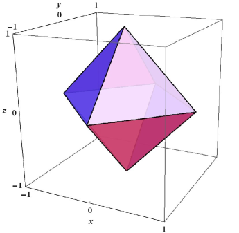
Figure 5: Three-dimensional plot of the octahedron with the vertices $\pm\vec{e}_{x}$, $\pm\vec{e}_{y}$, $\pm\vec{e}_{z}$.

In this way, $R_{x}$ is a symmetry rotation through $90^{\circ}$ about the four-fold axis $\vec{e}_{x}$ of the octahedron. But then, trivially, also $A=R_{x}^{2}$ is a symmetry rotation through $180^{\circ}$ about the same axis, and $E$ rotates the octahedron about $120^{\circ}$ through the axis given by equation (169). Having seen that $A$, $E$ and $R_{x}$, and thus also $R_{t}$, are symmetry rotations of the octahedron defined above via its vertices and knowing that $A$, $E$ and $R_{t}$ generate $S_{4}$ as a rotation group, we have indeed demonstrated the isomorphism $O\cong S_{4}$. Explicitly, it is given by

$$s=(123)\mapsto E,\quad k_{1}=(12)(34)\mapsto A,\quad t=(12)\mapsto R_{t}.$$ (189)

Having established the isomorphism (189), in the following, we will—for the sake of simplicity—use the notation of $S_{4}$ as introduced in section 4. In section 4.2 it was shown that $S_{4}$ is generated by $A_{4}$, which is itself generated by $k_{1}=(12)(34)$ and $s=(123)$, and the transposition $t=(12)$. Theorem 4.2 tells us that the classes of $S_{n}$ correspond to the different cycle structures. Equation (89) shows the five different cycle structures of the elements of $S_{4}$. We can model a four-cycle after $R_{x}$:

$$r:=s^{-1}k_{1}st=(1423).$$ (190)

We denote the classes of $S_{4}$, in the order of equation (89), by specifying one element of each class:

$$C_{1}(e),\enspace C_{2}(t),\enspace C_{3}(k_{1}),\enspace C_{4}(s),\enspace C_{5}(r).$$ (191)

Using the generators of $S_{4}$ it is easy to calculate $(\#C)$ and $\mathrm{ord}\,C$ to see the correspondence with the list of symmetry rotations (187)—see also table 8. Also $S_{4}$ is a favoured group for model building–see for instance [35]

Now we compute the irreps of $O\cong S_{4}$. We already have the representation of $S_{4}$ as a three-dimensional rotation group, i.e. as the octahedral group. Denoting this irrep by $\mathbf{3}$, in summary it is given by

$$\mathbf{3}:\quad t\mapsto R_{t}=\begin{pmatrix}-1&0&0\\ 0&0&-1\\ 0&-1&0\end{pmatrix},\quad k_{1}\mapsto A=\begin{pmatrix}1&0&0\\ 0&-1&0\\ 0&0&-1\end{pmatrix},\quad s\mapsto E=\begin{pmatrix}0&1&0\\ 0&0&1\\ 1&0&0\end{pmatrix}.$$ (192)

Theorem 4.9 tells us that there are only two one-dimensional irreps, namely

$$\begin{array}[]{clcc}\mathbf{1}:&t\mapsto 1,&k_{1}\mapsto 1,&s\mapsto 1,\\ \mathbf{1}^{\prime}:&t\mapsto-1,&k_{1}\mapsto 1,&s\mapsto 1.\end{array}$$ (193)

Then we obtain another three-dimensional irrep via

$$\mathbf{3}^{\prime}:=\mathbf{1}^{\prime}\otimes\mathbf{3}.$$ (194)

Since $S_{4}$ possesses five classes, one irrep is missing. Using theorem 3.31 we find its dimension to be two:

$$24=2\times 1^{2}+2\times 3^{2}+d^{2}\;\Rightarrow\;d=2.$$ (195)

The origin of this two-dimensional irrep can be understood from equation (105). Since Klein’s four-group $K$ is a normal subgroup of $S_{4}$, all irreps of

$$S_{4}/K\cong\mathbbm{Z}_{3}\rtimes\mathbbm{Z}_{2}\cong S_{3}$$ (196)

are irreps of $S_{4}$ too [25]. The identity element of $S_{4}/K$ is $K$, thus $k_{1}\in K$ must be mapped onto $\mathbbm{1}_{2}$. The representation matrices of $s$ and $t$ follow from the representation of $S_{3}$ as a three-dimensional rotation group—see equations (96) and (97):

$$\mathbf{2}:\quad t\mapsto\begin{pmatrix}0&1\\ 1&0\end{pmatrix},\quad k_{1}\mapsto\begin{pmatrix}1&0\\ 0&1\end{pmatrix},\quad s\mapsto\frac{1}{2}\begin{pmatrix}-1&-\sqrt{3}\\ \sqrt{3}&-1\end{pmatrix}.$$ (197)

With a basis transformation one can make the representation matrix of $s$ diagonal without altering the other two representation matrices:

$$\mathbf{2}:\quad t\mapsto\begin{pmatrix}0&1\\ 1&0\end{pmatrix},\quad k_{1}\mapsto\begin{pmatrix}1&0\\ 0&1\end{pmatrix},\quad s\mapsto\begin{pmatrix}\omega&0\\ 0&\omega^{2}\end{pmatrix}\quad\mbox{with}\quad\omega=e^{2\pi i/3}.$$ (198)

Sometimes this form of the $\mathbf{2}$ is useful. We now have all information needed in order to compute the character table of $S_{4}$, which is depicted in table 8. We want to mention that $S_{4}$ is quite popular as a flavour group—see for instance [25, 35] and references in [36].

$O\cong S_{4}$	$C_{1}(e)$	$C_{2}(t)$	$C_{3}(k_{1})$	$C_{4}(s)$	$C_{5}(r)$
(# $C$)	$(1)$	$(6)$	$(3)$	$(8)$	$(6)$
$\mbox{ord}\,(C)$	$1$	$2$	$2$	$3$	$4$
$\mathbf{1}$	$1$	$1$	$1$	$1$	$1$
$\mathbf{1}^{\prime}$	$1$	$-1$	$1$	$1$	$-1$
$\mathbf{2}$	$2$	$0$	$2$	$-1$	$0$
$\mathbf{3}$	$3$	$-1$	$-1$	$0$	$1$
$\mathbf{3}^{\prime}$	$3$	$1$	$-1$	$0$	$-1$

Table 8: The character table of $O\cong S_{4}$.

As an example for tensor products of irreps of $S_{4}$ we compute $\mathbf{3}\otimes\mathbf{3}$. Taking advantage of the character table 8 we obtain

$$\mathbf{3}\otimes\mathbf{3}=\mathbf{1}\oplus\mathbf{2}\oplus\mathbf{3}\oplus\mathbf{3}^{\prime}.$$ (199)

Since $T$ is a subgroup of $O$, equation (199) must be related to equation (177). Indeed, with the vectors defined in equation (178), the first two summands on the right-hand side of equation (199) are obtained in the following way:

$$\mathbf{1}:\;\;\mathcal{B}_{0},\quad\mathbf{2}:\;\;\mathcal{B}_{1},\;\mathcal{B}_{2}.$$ (200)

With this basis the $\mathbf{2}$ emerges in the form (198), which clearly shows that the $\mathbf{2}$ is composed of $\mathbf{1}^{(1)}$ and $\mathbf{1}^{(2)}$ of $T$. For the three-dimensional irreps one now has to use the symmetrized and antisymmetrized bases:

$$\frac{1}{\sqrt{2}}\left(e_{2}\otimes e_{3}\pm e_{3}\otimes e_{2}\right),\quad\frac{1}{\sqrt{2}}\left(e_{3}\otimes e_{1}\pm e_{1}\otimes e_{3}\right),\quad\frac{1}{\sqrt{2}}\left(e_{1}\otimes e_{2}\pm e_{2}\otimes e_{1}\right).$$ (201)

The plus sign refers to the $\mathbf{3}^{\prime}$ and the minus sign to the $\mathbf{3}$.

Now we move on to $\widetilde{O}$, the double cover of $O$. The generators of $\widetilde{O}$ are

$$\tilde{t}:=U(\pi,\vec{n}_{2}),\quad\tilde{k}_{1}:=-U(\pi,\vec{e}_{x}),\quad\tilde{s}:=U(2\pi/3,\vec{n}_{3})$$ (202)

with

$$\vec{n}_{2}=\frac{1}{\sqrt{2}}\left(\begin{array}[]{c}0\\ 1\\ -1\end{array}\right),\quad\vec{n}_{3}=-\frac{1}{\sqrt{3}}\left(\begin{array}[]{c}1\\ 1\\ 1\end{array}\right).$$ (203)

Equation (202) can be conceived as the defining irrep of $\widetilde{O}$ which explicitly is given by

$$\widetilde{\mathbf{2}}:\quad\tilde{t}=\frac{1}{\sqrt{2}}\begin{pmatrix}i&-1\\ 1&-i\end{pmatrix},\quad\tilde{k}_{1}=\begin{pmatrix}0&i\\ i&0\end{pmatrix},\quad\tilde{s}=\frac{1}{2}\left(\begin{array}[]{rc}1+i&1+i\\ -1+i&1-i\end{array}\right).$$ (204)

In the further discussion we will also utilize the elements

$$\tilde{r}={\tilde{s}}^{-1}\tilde{k}_{1}\tilde{s}\tilde{t}=\frac{1}{\sqrt{2}}\left(\begin{array}[]{rr}1&-i\\ -i&1\end{array}\right)\quad\mbox{and}\quad\tilde{k}_{2}=\tilde{s}\tilde{k}_{1}{\tilde{s}}^{-1}=\left(\begin{array}[]{cc}i&0\\ 0&-i\end{array}\right).$$ (205)

In order to find all irreps of $\widetilde{O}$ and the character table, we need to know the classes. We proceed in the same way as we did for the classes of $\widetilde{T}$. We take over the classes $C_{1}(\mathbbm{1}_{2})$, $C_{3}(\tilde{t})$, $C_{4}(\tilde{k}_{1})$, $C_{5}(\tilde{s})$ and $C_{7}(\tilde{r})$ from the octahedral group. Because of

$$\mathrm{Tr}\,\mathbbm{1}_{2}\neq 0,\enspace\mathrm{Tr}\,\tilde{s}\neq 0,\enspace\mathrm{Tr}\,\tilde{r}\neq 0$$ (206)

we find in the case of $\widetilde{O}$ three more classes:

$$C_{2}(-\mathbbm{1}_{2}),\enspace C_{6}(-\tilde{s})\quad\mbox{and}\quad C_{8}(-\tilde{r}).$$ (207)

The relations

$$\tilde{k}_{1}\tilde{t}{\tilde{k}_{1}}^{-1}=-\tilde{t}\quad\mbox{and}\quad\tilde{k}_{2}\tilde{k}_{1}{\tilde{k}_{2}}^{-1}=-\tilde{k}_{1}$$ (208)

demonstrate that there are no further classes. Since $\widetilde{O}$ possesses eight conjugacy classes, it also possesses eight inequivalent irreps. We already know six of them, namely the five irreps of $O$ and the defining irrep (204). The dimensions of the unknown irreps can be computed by means of theorem 3.31:

$$48=2\times 1^{2}+2\times 2^{2}+2\times 3^{2}+d_{7}^{2}+d_{8}^{2}\;\Rightarrow\;d_{7}=2,\quad d_{8}=4.$$ (209)

The missing two-dimensional irrep is given by

$${\widetilde{\mathbf{2}}}^{\prime}:=\mathbf{1}^{\prime}\otimes\widetilde{\mathbf{2}}.$$ (210)

Note that we keep the notation $\mathbf{1}^{\prime}$ for the one-dimensional non-trivial irrep of $O$. Keeping also the notation for the $\mathbf{2}$, one can check that the tensor product $\mathbf{2}\otimes\widetilde{\mathbf{2}}$ fulfills

$$\langle\chi^{(\mathbf{2}\otimes\widetilde{\mathbf{2}})}|\chi^{(\mathbf{2}\otimes\widetilde{\mathbf{2}})}\rangle=1.$$ (211)

Then we know from theorem 3.40 that

$$\widetilde{\mathbf{4}}:=\mathbf{2}\otimes\widetilde{\mathbf{2}}\quad\mbox{is irreducible}.$$ (212)

Having obtained all classes and irreps we can compute the character table which is presented in table 9.

$\widetilde{O}$	$C_{1}(\mathbbm{1}_{2})$	$C_{2}(-\mathbbm{1}_{2})$	$C_{3}(\tilde{t})$	$C_{4}(\tilde{k}_{1})$	$C_{5}(\tilde{s})$	$C_{6}(-\tilde{s})$	$C_{7}(\tilde{r})$	$C_{8}(-\tilde{r})$
(# $C$)	$(1)$	$(1)$	$(12)$	$(6)$	$(8)$	$(8)$	$(6)$	$(6)$
$\mbox{ord}\,(C)$	$1$	$2$	$4$	$4$	$6$	$3$	$8$	$8$
$\mathbf{1}$	$1$	$1$	$1$	$1$	$1$	$1$	$1$	$1$
$\mathbf{1}^{\prime}$	$1$	$1$	$-1$	$1$	$1$	$1$	$-1$	$-1$
$\mathbf{2}$	$2$	$2$	$0$	$2$	$-1$	$-1$	$0$	$0$
$\widetilde{\mathbf{2}}$	$2$	$-2$	$0$	$0$	$1$	$-1$	$\sqrt{2}$	$-\sqrt{2}$
${\widetilde{\mathbf{2}}}^{\prime}$	$2$	$-2$	$0$	$0$	$1$	$-1$	$-\sqrt{2}$	$\sqrt{2}$
$\mathbf{3}$	$3$	$3$	$-1$	$-1$	$0$	$0$	$1$	$1$
$\mathbf{3}^{\prime}$	$3$	$3$	$1$	$-1$	$0$	$0$	$-1$	$-1$
$\widetilde{\mathbf{4}}$	$4$	$-4$	$0$	$0$	$-1$	$1$	$0$	$0$

Table 9: The character table of $\widetilde{O}$. The irreps without tilde correspond to the irreps of $O$.

5.3.5 The icosahedral group and its double cover

The icosahedral group $I$ is the rotation symmetry group of both the regular icosahedron and the regular dodecahedron [19]. In order to construct the classes of the icosahedral group, we once more make use of the rules presented in section 5.2. The regular icosahedron possesses twelve vertices, thirty edges and twenty faces, which are unilateral triangles. The denomination of this solid follows from the Greek word for “twenty.” Using a three-dimensional model of an icosahedron, one can easily find the different types of rotation axes and their properties:

• Type 1: Axes pointing through two opposite vertices. The icosahedron has six equivalent five-fold axes of this type. Since these axes are two-sided, with any element also its inverse belongs to the same class. Therefore, we find two classes, the class of rotations through $\pm 72^{\circ}$ and the class of rotations through $\pm 144^{\circ}$, containing twelve elements each.

• Type 2: Axes connecting the centers of two opposite edges. Fifteen equivalent two-fold two-sided axes are of this type, giving rise to a single conjugacy class containing fifteen elements.

• Type 3: Axes pointing through the centers of two opposite faces. This type of axes corresponds to ten equivalent three-fold axes. One finds that these axes are also two-sided, so we obtain a single conjugacy class consisting of twenty elements which are rotations through $\pm 120^{\circ}$.

Thus we arrive at the following list of classes of $I$:

$$\begin{matrix}\mbox{axis type}&0&1&1&2&3\\ (\#C)&(1)&(12)&(12)&(15)&(20)\\ \mathrm{ord}\,C&1&5&5&2&3\end{matrix}$$ (213)

The class of the identity element is denoted by axis type 0. From the above list we find $\mbox{ord}\,I=60$.

In the previous section we have already seen that the tetrahedral and the octahedral groups are isomorphic to the permutation groups $A_{4}$ and $S_{4}$, respectively. Furthermore, in section 4.2, we have derived a representation of $A_{5}$ as a three-dimensional rotation group of order 60. Since also the classes (213) match the classes of $A_{5}$—see equation (95) and the subsequent discussion there, it is suggestive to assume that $A_{5}$ is isomorphic to $I$. That this is the case can be proven by constructing the vertices of the icosahedron from the rotational representation of $A_{5}$. This is done in appendix D.

Having established that the rotation symmetry group $I$ of a regular icosahedron is isomorphic to $A_{5}$, it is then clear from the material in section 4.2 that the concrete realization of this isomorphism is given by

$$s=(123)\mapsto E,\quad k_{1}=(12)(34)\mapsto A,\quad k_{4}=(12)(45)\mapsto W,$$ (214)

where $A$ and $E$ are defined in equation (100), and $W$ is defined in equation (111).

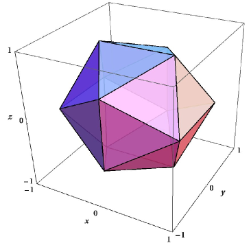
Figure 6: Three-dimensional plot of the icosahedron obtained by interpreting the vectors of equation (D2) as its vertices.

Now we want to construct the irreps and the character table of $A_{5}$. First we determine the classes. According to the discussion following equation (95) we immediately find the two non-trivial classes $C_{2}(s)$ and $C_{3}(k_{1})$. The other two classes are the classes consisting of five-cycles. Since $k_{1}k_{4}s=(12453)$ and $k_{4}k_{1}s=(12543)$ are related via

$$(45)(12453)(45)^{-1}=(12543)$$ (215)

with $(45)\not\in A_{5}$, the two remaining classes are

$$C_{4}(k_{1}k_{4}s)\quad\mbox{and}\quad C_{5}(k_{4}k_{1}s).$$ (216)

Because $s$, $k_{1}$ and $k_{4}$ generate an element of each conjugacy class, they generate the whole group—see corollary 3.5. In this way we have found an alternative proof that $A_{5}$ is generated by the permutations (214). The two inequivalent three-dimensional representations of $A_{5}$ constructed in section 4.2 are given by

$$\begin{array}[]{cccl}\mathbf{3}:&s\mapsto E,&k_{1}\mapsto A,&k_{4}\mapsto W,\\ \mathbf{3}^{\prime}:&s\mapsto E,&k_{1}\mapsto A,&k_{4}\mapsto W^{\prime},\end{array}$$ (217)

where $A$, $E$ and $W$, $W^{\prime}$ are defined in equations (100) and (111), respectively. The dimensions of the missing non-trivial irreps follow from

$$60=1^{2}+2\times 3^{2}+d_{4}^{2}+d_{5}^{2}\;\Rightarrow\;d_{4}=4,\enspace d_{5}=5.$$ (218)

The five-dimensional irrep corresponds to the five-dimensional $SO(3)$-irrep, which can be computed from equation (70). Therefore, in terms of irreps of $A_{5}$ we find

$$\mathbf{3}\otimes\mathbf{3}=\mathbf{1}\oplus\mathbf{3}\oplus\mathbf{5}.$$ (219)

The bases of the one and three-dimensional invariant subspaces are provided by equations (68) and (69), respectively. Using these bases one can easily reduce $\mathbf{3}\otimes\mathbf{3}$ and construct the $\mathbf{5}$ explicitly. However, here we confine ourselves to the character $\chi^{(\textbf{5})}$, which—according to equation (219)—is given by

$$\chi^{(\mathbf{5})}=\chi^{(\mathbf{3})}\times\chi^{(\mathbf{3})}-\chi^{(\mathbf{3})}-\chi^{(\mathbf{1})}.$$ (220)

Using the relation (58), one finds that of the irreps we have already constructed only the $\mathbf{5}$ is contained in $\mathbf{3}\otimes\mathbf{3}^{\prime}$. Therefore, the other irrep in the tensor product can only be the $\mathbf{4}$. Its character is thus given by

$$\chi^{(\mathbf{4})}=\chi^{(\mathbf{3})}\times\chi^{(\mathbf{3}^{\prime})}-\chi^{(\mathbf{5})}.$$ (221)

Having completed the computation of characters, we are in a position to write down the character table of $I\cong A_{5}$—see table 10. This flavour group has for instance been used in [37] for model building.

$I\cong A_{5}$	$C_{1}(e)$	$C_{2}(s)$	$C_{3}(k_{1})$	$C_{4}(k_{1}k_{4}s)$	$C_{5}(k_{4}k_{1}s)$
(# $C$)	$(1)$	$(20)$	$(15)$	$(12)$	$(12)$
$\mbox{ord}\,(C)$	$1$	$3$	$2$	$5$	$5$
$\mathbf{1}$	$1$	$1$	$1$	$1$	$1$
$\mathbf{3}$	$3$	$0$	$-1$	$-\mu_{2}$	$-\mu_{1}$
$\mathbf{3}^{\prime}$	$3$	$0$	$-1$	$-\mu_{1}$	$-\mu_{2}$
$\mathbf{4}$	$4$	$1$	$0$	$-1$	$-1$
$\mathbf{5}$	$5$	$-1$	$1$	$0$	$0$

Table 10: The character table of $I\cong A_{5}$ with $\mu_{1}=\frac{-1+\sqrt{5}}{2}$, $\mu_{2}=\frac{-1-\sqrt{5}}{2}$.

Now we discuss the double cover $\widetilde{I}$. Using equation (118), we compute the rotation axes and angles for $W$ and $W^{\prime}$. We obtain $\alpha=180^{\circ}$ for both $W$ and $W^{\prime}$, and the axes

$$\vec{w}=\frac{1}{2}\left(\begin{array}[]{c}1\\ \mu_{2}\\ \mu_{1}\end{array}\right)\quad\mbox{and}\quad{\vec{w}}^{\prime}=\frac{1}{2}\left(\begin{array}[]{c}1\\ \mu_{1}\\ \mu_{2}\end{array}\right),$$ (222)

respectively. Inserting this result into equation (120), we define

$$\tilde{k}_{4}:=U(\pi,\vec{w})=\frac{1}{2}\begin{pmatrix}-i\mu_{1}&-\mu_{2}-i\\ \mu_{2}-i&i\mu_{1}\end{pmatrix}$$ (223)

and

$$\tilde{k}_{4}^{\prime}:=U(\pi,{\vec{w}}^{\prime})=\frac{1}{2}\begin{pmatrix}-i\mu_{2}&-\mu_{1}-i\\ \mu_{1}-i&i\mu_{2}\end{pmatrix}.$$ (224)

Together with $\tilde{s}$ and $\tilde{k}_{1}$ defined in equation (202), we obtain two faithful inequivalent two-dimensional irreps of $\widetilde{I}$:

$$\begin{array}[]{cccl}\widetilde{\mathbf{2}}:&\tilde{s}\mapsto\tilde{s},&\tilde{k}_{1}\mapsto\tilde{k}_{1},&\tilde{k}_{4}\mapsto\tilde{k}_{4},\\ \widetilde{\mathbf{2}}^{\prime}:&\tilde{s}\mapsto\tilde{s},&\tilde{k}_{1}\mapsto\tilde{k}_{1},&\tilde{k}_{4}\mapsto\tilde{k}_{4}^{\prime}.\end{array}$$ (225)

The classes are easily deduced from the classes of $A_{5}$—see table 10. In this way, we find $C_{1}(\mathbbm{1}_{2})$, $C_{2}(-\mathbbm{1}_{2})$, $C_{3}(\tilde{s})$, $C_{4}(-\tilde{s})$. Defining

$$\tilde{y}:=\tilde{s}\tilde{k}_{1}\tilde{s}^{-1}=\begin{pmatrix}i&0\\ 0&-i\end{pmatrix},$$ (226)

we deduce that

$$\tilde{y}\tilde{k}_{1}{\tilde{y}}^{-1}=-\tilde{k}_{1}\;\Rightarrow\;C_{5}(\tilde{k}_{1})=C_{5}(-\tilde{k}_{1}).$$ (227)

Since the traces of $\tilde{k}_{1}\tilde{k}_{4}\tilde{s}$ and $\tilde{k}_{4}\tilde{k}_{1}\tilde{s}$ are non-zero, the classes corresponding to the two remaining classes of $A_{5}$ do not coincide with their negatives. Thus there are nine conjugacy classes and consequently also nine inequivalent irreps. We already know seven of them, namely the five irreps of $A_{5}$ and the two irreps (225). We denote the dimensions of the two remaining irreps by $d_{7}$ and $d_{9}$, already anticipating their positions in the character table. They are determined by

$$120=1^{2}+2\times 3^{2}+4^{2}+5^{2}+2\times 2^{2}+d_{7}^{2}+d_{9}^{2}\;\Rightarrow\,d_{7}=4,\enspace d_{9}=6.$$ (228)

Using the characters of the already constructed irreps, one can compute that

$$\widetilde{\mathbf{6}}:=\widetilde{\mathbf{2}}^{\prime}\otimes\mathbf{3}\cong\widetilde{\mathbf{2}}\otimes\mathbf{3}^{\prime}$$ (229)

is irreducible. Finally, the character of $\widetilde{\mathbf{4}}$ can be found from

$$\widetilde{\mathbf{2}}\otimes\mathbf{3}=\widetilde{\mathbf{2}}\oplus\widetilde{\mathbf{4}}.$$ (230)

The character table of $\widetilde{I}$ is presented in table 11. For the tensor products of irreps see [38]. An alternative discussion of $\widetilde{I}$ is presented in [39].

$\widetilde{I}$	$C_{1}(\mathbbm{1}_{2})$	$C_{2}(-\mathbbm{1}_{2})$	$C_{3}(\tilde{s})$	$C_{4}(-\tilde{s})$	$C_{5}(\tilde{k}_{1})$	$C_{6}(\tilde{k}_{1}\tilde{k}_{4}\tilde{s})$​	$C_{7}(-\tilde{k}_{1}\tilde{k}_{4}\tilde{s})$​	$C_{8}(\tilde{k}_{4}\tilde{k}_{1}\tilde{s})$​	$C_{9}(-\tilde{k}_{4}\tilde{k}_{1}\tilde{s})$
(# $C$)	$(1)$	$(1)$	$(20)$	$(20)$	$(30)$	$(12)$	$(12)$	$(12)$	$(12)$
$\mbox{ord}\,(C)$	$1$	$2$	$6$	$3$	$4$	$10$	$5$	$10$	$5$
$\mathbf{1}$	$1$	$1$	$1$	$1$	$1$	$1$	$1$	$1$	$1$
$\widetilde{\mathbf{2}}$	$2$	$-2$	$1$	$-1$	$0$	$-\mu_{2}$	$\mu_{2}$	$-\mu_{1}$	$\mu_{1}$
${\widetilde{\mathbf{2}}}^{\prime}$	$2$	$-2$	$1$	$-1$	$0$	$-\mu_{1}$	$\mu_{1}$	$-\mu_{2}$	$\mu_{2}$
$\mathbf{3}$	$3$	$3$	$0$	$0$	$-1$	$-\mu_{2}$	$-\mu_{2}$	$-\mu_{1}$	$-\mu_{1}$
$\mathbf{3}^{\prime}$	$3$	$3$	$0$	$0$	$-1$	$-\mu_{1}$	$-\mu_{1}$	$-\mu_{2}$	$-\mu_{2}$
$\mathbf{4}$	$4$	$4$	$1$	$1$	$0$	$-1$	$-1$	$-1$	$-1$
$\widetilde{\mathbf{4}}$	$4$	$-4$	$-1$	$1$	$0$	$1$	$-1$	$1$	$-1$
$\mathbf{5}$	$5$	$5$	$-1$	$-1$	$1$	$0$	$0$	$0$	$0$
$\widetilde{\mathbf{6}}$	$6$	$-6$	$0$	$0$	$0$	$-1$	$1$	$-1$	$1$

Table 11: The character table of $\widetilde{I}$ with $\mu_{1}=\frac{-1+\sqrt{5}}{2}$, $\mu_{2}=\frac{-1-\sqrt{5}}{2}$. The irreps without tilde correspond to the irreps of $I$.

6 The finite subgroups of $SU(3)$

6.1 Classification

According to [24, 40] the finite subgroups of $SU(3)$ can be classified into the following types:

1. Groups of diagonal matrices corresponding to Abelian groups.

2. Groups corresponding to linear transformations of two variables. Up to basis transformations such $SU(3)$-matrices have the form

   $$\left(\begin{array}[]{cc}\det A^{*}&0_{1\times 2}\\ 0_{2\times 1}&A\end{array}\right)\mbox{with}\quad A\in U(2).$$ (231)

3. The groups $C(n,a,b)$ generated by the matrices

   $$E=\begin{pmatrix}0&1&0\\ 0&0&1\\ 1&0&0\\ \end{pmatrix}\quad\mbox{and}\quad F(n,a,b)=\begin{pmatrix}\eta^{a}&0&0\\ 0&\eta^{b}&0\\ 0&0&\eta^{-a-b}\\ \end{pmatrix},$$ (232)

   where $n$ is a positive integer, $\eta=\exp(2\pi i/n)$ and integers $a$, $b$ with $0\leq a,b\leq n-1$.

4. The groups $D(n,a,b;d,r,s)$ generated by $E$ and $F(n,a,b)$ of equation (232) and

   $$\tilde{G}(d,r,s)=\left(\begin{array}[]{ccc}\delta^{r}&0&0\\ 0&0&\delta^{s}\\ 0&-\delta^{-r-s}&0\end{array}\right),$$ (233)

   where $d$ is a positive integer, $\delta=\exp(2\pi i/d)$ and integers $r$, $s$ with $0\leq r,s\leq d-1$.

5. The “exceptional” finite subgroups of $SU(3)$, denoted by $\Sigma(60)$, $\Sigma(168)$, ${\Sigma(36\times 3)}$, $\Sigma(72\times 3)$, $\Sigma(216\times 3)$ and $\Sigma(360\times 3)$.

For completeness we should add to the groups of type E the direct products $\Sigma(60)\times\mathbbm{Z}_{3}$ and $\Sigma(168)\times\mathbbm{Z}_{3}$. A brief history of the classification of the finite subgroups of $SU(3)$ can be found in the introduction of [41].

Groups of type A:

Such groups are Abelian and, therefore, they must have a structure conforming to theorems 3.15 and 3.16. However, knowing that these groups are subgroups of $SU(3)$ a more specific statement can be made, as proven in [41].

Theorem 6.1.

Every Abelian finite subgroup $G$ of $SU(3)$ is isomorphic to $\mathbbm{Z}_{m}\times\mathbbm{Z}_{n}$ where $m$ is the maximum of the orders of the elements of $G$ and $n$ is a divisor of $m$.

Groups of type B:

These groups contain all $SU(2)$ subgroups and the dihedral groups, which have been discussed already in section 5. In addition, they comprise the genuine $U(2)$ subgroups, not treated in this review.

Groups of type C:

The structure of groups of type C can be understood in the following way. We denote the subgroup of diagonal matrices of $C(n,a,b)$ by $N(n,a,b)$. Because of

$$E\,\mbox{diag}\,(\alpha,\beta,\gamma)E^{-1}=\mbox{diag}\,(\beta,\gamma,\alpha)$$ (234)

it is obvious that this subgroup is a normal subgroup, whence it follows that every element $g\in C(n,a,b)$ can be written in the form $g=FE^{k}$, with $F\in N(n,a,b)$ and $k=0,1,2$. It is easy to see that $N(n,a,b)$ is generated by

$$F(n,a,b)\quad\mbox{and}\quad EF(n,a,b)E^{-1}=\mbox{diag}\,(\eta^{b},\eta^{-a-b},\eta^{a}).$$ (235)

Armed with this knowledge we can write the multiplication rule of two group elements as

$$\left(F_{1}E^{k_{1}}\right)\left(F_{2}E^{k_{2}}\right)=\left(F_{1}E^{k_{1}}F_{2}E^{-k_{1}}\right)E^{k_{1}+k_{2}}.$$ (236)

Therefore, since $E^{3}=\mathbbm{1}$, the groups of type C can be characterized as

$$C(n,a,b)\cong N(n,a,b)\rtimes\mathbbm{Z}_{3},$$ (237)

where the homomorphism of the semidirect product, $\varphi:\mathbbm{Z}_{3}\to\mbox{Aut}(N(n,a,b))$, is read off from equation (236):

$$\varphi(E^{k})F=E^{k}FE^{-k}.$$ (238)

According to theorem 6.1, there are positive integers $m$ and $p$ such that

$$N(n,a,b)\cong\mathbbm{Z}_{m}\times\mathbbm{Z}_{p}.$$ (239)

In [41] a set of rules has been derived which allows to compute the integers $m$ and $p$ from $n,a,b$. The value of $m$ is found to be the smallest positive natural number such that

$$(\eta^{a})^{m}=(\eta^{b})^{m}=1.$$ (240)

The parameter $p$ can be determined following a prescription, which involves another parameter $t$. Starting with $p^{\prime}=1$ we go through all divisors of $m$ and check whether there exists a $t\in\{1,...,m/p^{\prime}-1\}$ such that

$$p^{\prime}(b-at)\,\mathrm{mod}\,n=0\quad\mbox{and}\quad p^{\prime}(a+b(1+t))\,\mathrm{mod}\,n=0$$ (241)

The smallest $p^{\prime}$ for which such a $t$ exists is our sought-for value of $p$—for details see [41].

As proven in appendix E, the groups of type C can only have irreps of dimension one and three.

The groups $C(n,a,b)$ contain the important series

$$C(n,1,0)\equiv\Delta(3n^{2})\cong(\mathbbm{Z}_{n}\times\mathbbm{Z}_{n})\rtimes\mathbbm{Z}_{3},$$ (242)

which will be discussed in section 6.2. Another series is $T_{n}$, given by $C(n,1,a)$ with $1+a+a^{2}=0\,\mbox{mod}\,n$. This is possible only for specific $n$, as we will discuss in section 6.3. The smallest group of type C that does not belong to $\Delta(3n^{2})$ and $T_{n}$ and that is not a direct product is

$$C(9,1,1)\cong(\mathbbm{Z}_{9}\times\mathbbm{Z}_{3})\rtimes\mathbbm{Z}_{3}$$ (243)

with 81 elements [41]. Apart from $A_{4}\cong\Delta(12)$ which has already been discussed, among the groups of type C which have been used as flavour symmetries there are $\Delta(27)$ [42], $\Delta(75)$ [43], $T_{7}$ [44, 45, 46] and $T_{13}$ [47].

Groups of type D:

To understand the structure of $D(n,a,b;d,r,s)$, it is useful to switch to a new set of generators [48, 49]. The derivation of this new set is performed in appendix F. With

$$F_{r}=\mbox{diag}\,\left(-\delta^{-r},\,-\delta^{-r},\,\delta^{2r}\right),\quad F^{\prime}_{t}=\mbox{diag}\,(\delta^{-t},\,\delta^{-t},\,\delta^{2t})\quad\mbox{with}\quad t=r-s$$ (244)

and

$$B=\left(\begin{array}[]{rrr}-1&0&0\\ 0&0&-1\\ 0&-1&0\end{array}\right),$$ (245)

it is given by

$$F(n,a,b),\;F_{r},\;F^{\prime}_{t},\;E,\;B.$$ (246)

This set of generators clearly shows the structure of the groups $D(n,a,b;d,r,s)$. The matrices $E$ and $B$ obviously generate a subgroup isomorphic to $S_{3}$. Moreover, the group $D(n,a,b;d,r,s)$ has a normal subgroup $N(n,a,b;d,r,s)$ of diagonal matrices which consists of $F(n,a,b)$, $F_{r}$, $F^{\prime}_{t}$, the matrices obtained from these three by similarity transformations with $E$ and $B$—see equations (234) and

$$B\,\mbox{diag}\,(\alpha,\beta,\gamma)B^{-1}=\mbox{diag}\,(\alpha,\gamma,\beta),$$ (247)

and all products thereof. Furthermore, it follows that every $g\in D(n,a,b;d,r,s)$ can be written as

$$g=FE^{k}B^{l}\quad\mbox{with}\quad F\in N(n,a,b;d,r,s),\;k=0,1,2,\;\;l=0,1.$$ (248)

So we find that groups of type D have the structure of a semidirect product:

$$D(n,a,b;d,r,s)\cong N(n,a,b;d,r,s)\rtimes S_{3}.$$ (249)

Finally we can exploit theorem 6.1 which tells us that $N(n,a,b;d,r,s)$ is a direct product of two cyclic groups with suitably chosen orders $m$ and $p$, where $p$ is a divisor of $m$. Therefore, we end up with

$$D(n,a,b;d,r,s)\cong\left(\mathbbm{Z}_{m}\times\mathbbm{Z}_{p}\right)\rtimes S_{3}.$$ (250)

The dimensions of the irreps of the groups of type D are quite restricted, only one, two, three and six are possible—see the proof in appendix G. In essence this follows from the semidirect product (249).

The groups of type D comprise the well-known series of dihedral-like groups

$$D(n,0,1;2,1,1)\equiv\Delta(6n^{2})\cong\left(\mathbbm{Z}_{n}\times\mathbbm{Z}_{n}\right)\rtimes S_{3},$$ (251)

which will be discussed in section 6.4. Apart from $\Delta(6)\cong S_{3}$ and $\Delta(24)\cong S_{4}$, a group of type D used as flavor symmetry is $\Delta(54)$ [50]. The smallest group of type D that is not a direct product or a group of the $\Delta(6n^{2})$-series is [41]

$$D(9,1,1;2,1,1)\cong\left(\mathbbm{Z}_{9}\times\mathbbm{Z}_{3}\right)\rtimes S_{3}.$$ (252)

The first group, $\Sigma(60)$, of the “exceptional” finite subgroups of $SU(3)$ is identical with the icosahedral group and thus isomorphic to $A_{5}$ which has been discussed in sections 4.2 and 5.3.5. It is the smallest non-Abelian simple group. The other five “exceptional” groups will not be discussed in this review. For $\Sigma(168)$, which is the second smallest non-Abelian simple group, we refer the reader to [39, 51]. The groups denoted by $\Sigma(n\times 3)$ contain the center of $SU(3)$; an extensive discussion of the groups with $n=36,\,72,\,216$ can be found in [13].

6.2 The series $\Delta(3n^{2})$

We follow the discussion of [52] where the notation

$$a\equiv E,\quad c=\mbox{diag}\,(\eta,\,1,\,\eta^{-1}),\quad d=\mbox{diag}\,(\eta^{-1},\,\eta,\,1)$$ (253)

is used, with $\eta=\exp(2\pi i/n)$. This is a set of generators of $C(n,1,0)\equiv\Delta(3n^{2})$ because $c=F(n,1,0)$ and $d=E^{-1}F(n,1,0)E$. Actually, we could skip either $c$ or $d$ but keeping both makes the structure of $\Delta(3n^{2})$ more transparent, as pointed out in [52]. One can readily verify that the generators fulfill

$$a^{3}=c^{n}=d^{n}=e,\quad cd=dc,\quad\quad aca^{-1}=c^{-1}d^{-1},\quad ada^{-1}=c.$$ (254)

Thus $c$ and $d$ commute and each of them generates a $\mathbbm{Z}_{n}$, while the element $a$ generates a $\mathbbm{Z}_{3}$ and acts on $\mathbbm{Z}_{n}\times\mathbbm{Z}_{n}$. Therefore, $\Delta(3n^{2})$ is the semidirect product of $\mathbbm{Z}_{n}\times\mathbbm{Z}_{n}$ with $\mathbbm{Z}_{3}$ and its order is

$$\mbox{ord}\,\Delta(3n^{2})=3n^{2}.$$ (255)

We already know the first two members of this series: $\Delta(3)\cong\mathbbm{Z}_{3}$ and $\Delta(12)\cong A_{4}$. The latter statement is evident from equation (100).

By means of equation (254) it is nearly trivial to find the one-dimensional irreps. In these irreps $c$ and $d$ must be presented by the same number and, moreover, $c^{3}\mapsto 1$. Since also $c^{n}\mapsto 1$, we must distinguish if three is a divisor of $n$ or not:

$$\begin{array}[]{ccrcccl}\frac{n}{3}\not\in\mathbbm{N}&\Rightarrow&\mathbf{1}^{(p)}:&a\mapsto\omega^{p},&c\mapsto 1,&d\mapsto 1&(p=0,1,2),\\ \frac{n}{3}\in\mathbbm{N}&\Rightarrow&\mathbf{1}^{(p,q)}:&a\mapsto\omega^{p},&c\mapsto\omega^{q},&d\mapsto\omega^{q}&(p,q=0,1,2).\end{array}$$ (256)

Thus, if three is a divisor of $n$, there are nine inequivalent one-dimensional irreps, otherwise this number is three. Therefore, $\Delta(27)$ has nine, but $A_{4}\cong\Delta(12)$ has only three one-dimensional irreps.

Since $\Delta(3n^{2})$ is a group of type C, the remaining irreps must all have dimension three. The number of three-dimensional irreps is $(n^{2}-1)/3$ if three is not a divisor of $n$; otherwise their number is $(n^{2}-3)/3$. The three-dimensional irreps are given by [52]

$$\mathbf{3}^{(k,l)}:\quad a\mapsto E,\quad c\mapsto\mbox{diag}\,(\eta^{l},\,\eta^{k},\,\eta^{-k-l}),\quad d\mapsto\mbox{diag}\,(\eta^{-k-l},\,\eta^{l},\,\eta^{k})$$ (257)

with $k,l,=0,1,\ldots,n-1$. The defining irrep corresponds to $(k,l)=(0,1)$. The pair $(0,0)$ does not give an irrep; if three is a divisor of $n$, also $(\frac{n}{3},\frac{n}{3})$ and $(\frac{2n}{3},\frac{2n}{3})$ must be excluded. Moreover, for some pairs $(k,l)$ one obtains equivalent irreps. For a detailed discussion we refer the reader to [52].

We discuss the irreps of $\Delta(27)$ corresponding to $n=3$ in detail. Its nine one-dimensional irreps are known from equation (256). A minimal set of generators for the defining three-dimensional irrep is, for instance, given by

$$\Delta(27):\quad E\quad\mbox{and}\quad C:=\mbox{diag}\,(1,\,\omega,\,\omega^{2}),$$ (258)

where $E$ is defined in equation (232). Note that equation (258) can be considered as the representation $a\mapsto E$, $cd\mapsto C$. With $acda^{-1}=d^{-1}$ the representation matrices of $c$ and $d$ can be reconstructed. The classes are computed by using the relations

$$ECE^{-1}=\omega C,\quad CEC^{-1}=\omega^{2}E.$$ (259)

It convenient to define the set of matrices

$$\mathcal{Z}\equiv\{\mathbbm{1},\,\omega\mathbbm{1},\,\omega^{2}\mathbbm{1}\}$$ (260)

which corresponds to the center of $SU(3)$. With the abbreviation $\mathcal{Z}\cdot g\equiv\{g,\,\omega g,\,\omega^{2}g\}$, we can readily formulate the conjugacy classes [13]:

$$\begin{array}[]{llll}C_{1}=\{\mathbbm{1}\},&C_{2}=\{\omega\mathbbm{1}\},&C_{3}=\{\omega^{2}\mathbbm{1}\},&\\ C_{4}=\mathcal{Z}\cdot C,&C_{5}=\mathcal{Z}\cdot C^{2},&C_{6}=\mathcal{Z}\cdot E,&C_{7}=\mathcal{Z}\cdot E^{2},\\ C_{8}=\mathcal{Z}\cdot CE,&C_{9}=\mathcal{Z}\cdot C^{2}E^{2},&C_{10}=\mathcal{Z}\cdot C^{2}E,&C_{11}=\mathcal{Z}\cdot CE^{2}.\end{array}$$ (261)

Therefore, there are eleven inequivalent irreps. We already know the nine one-dimensional ones. The two remaining irreps must be three-dimensional due to

$$9\times 1^{2}+2\times 3^{2}=27$$ (262)

and are given by the defining irrep and its complex conjugate:

$$\begin{array}[]{ccc}\mathbf{3}:&E\mapsto E,&C\mapsto C,\\ \mathbf{3}^{*}:&E\mapsto E,&C\mapsto C^{*}.\end{array}$$ (263)

The character table of $\Delta(27)$ is found in table 12. Note that the one-dimensional irreps $\mathbf{1}^{(p,q)}$ are obtained by the mappings $E\mapsto\omega^{p}$, $C\mapsto\omega^{2q}$.

$\Delta(27)$	$C_{1}$	$C_{2}$	$C_{3}$	$C_{4}$	$C_{5}$	$C_{6}$	$C_{7}$	$C_{8}$	$C_{9}$	$C_{10}$	$C_{11}$
(# $C$)	(1)	(1)	(1)	(3)	(3)	(3)	(3)	(3)	(3)	(3)	(3)
$\mbox{ord}\,(C)$	1	3	3	3	3	3	3	3	3	3	3
$\mathbf{1}^{(0,0)}$	$1$	$1$	$1$	$1$	$1$	$1$	$1$	$1$	$1$	$1$	$1$
$\mathbf{1}^{(0,1)}$	$1$	$1$	$1$	$\omega^{2}$	$\omega$	$1$	$1$	$\omega^{2}$	$\omega$	$\omega$	$\omega^{2}$
$\mathbf{1}^{(0,2)}$	$1$	$1$	$1$	$\omega$	$\omega^{2}$	$1$	$1$	$\omega$	$\omega^{2}$	$\omega^{2}$	$\omega$
$\mathbf{1}^{(1,0)}$	$1$	$1$	$1$	$1$	$1$	$\omega$	$\omega^{2}$	$\omega$	$\omega^{2}$	$\omega$	$\omega^{2}$
$\mathbf{1}^{(1,1)}$	$1$	$1$	$1$	$\omega^{2}$	$\omega$	$\omega$	$\omega^{2}$	$1$	$1$	$\omega^{2}$	$\omega$
$\mathbf{1}^{(1,2)}$	$1$	$1$	$1$	$\omega$	$\omega^{2}$	$\omega$	$\omega^{2}$	$\omega^{2}$	$\omega$	$1$	$1$
$\mathbf{1}^{(2,0)}$	$1$	$1$	$1$	$1$	$1$	$\omega^{2}$	$\omega$	$\omega^{2}$	$\omega$	$\omega^{2}$	$\omega$
$\mathbf{1}^{(2,1)}$	$1$	$1$	$1$	$\omega^{2}$	$\omega$	$\omega^{2}$	$\omega$	$\omega$	$\omega^{2}$	$1$	$1$
$\mathbf{1}^{(2,2)}$	$1$	$1$	$1$	$\omega$	$\omega^{2}$	$\omega^{2}$	$\omega$	$1$	$1$	$\omega$	$\omega^{2}$
$\mathbf{3}$	$3$	$3\omega$	$3\omega^{2}$	$0$	$0$	$0$	$0$	$0$	$0$	$0$	$0$
$\mathbf{3}^{*}$	$3$	$3\omega^{2}$	$3\omega$	$0$	$0$	$0$	$0$	$0$	$0$	$0$	$0$

Table 12: Character table of $\Delta(27)$ with $\omega=\frac{-1+i\sqrt{3}}{2}$.

Finally we discuss tensor products of the irreps of $\Delta(27)$. Equation (259) tells us that $\omega\mathbbm{1}\mapsto 1$ in every one-dimensional irrep. Using this observation and denoting the characters of the one-dimensional irreps by $\chi^{(p,q)}$, we read off from table 12 that

$$\chi^{(p,q)}\times\chi^{(\mathbf{3})}=\chi^{(\mathbf{3})}\quad\mbox{and}\quad\chi^{(p,q)}\times\chi^{(\mathbf{3}^{*})}=\chi^{(\mathbf{3}^{*})},$$ (264)

whence we conclude

$$\mathbf{1}^{(p,q)}\otimes\mathbf{3}\cong\mathbf{3},\quad\mathbf{1}^{(p,q)}\otimes\mathbf{3}^{*}\cong\mathbf{3}^{*}.$$ (265)

We discuss one example of this equivalence, namely $p=1$, $q=0$. In this case the tensor product corresponds to the representation

$$E\mapsto\omega E,\quad C\mapsto C.$$ (266)

Then the basis transformation which demonstrates the equivalence

$$\mathbf{1}^{(1,0)}\otimes\mathbf{3}\cong\mathbf{3}$$ (267)

is provided by the matrix $C$ due to $C(\omega E)C^{-1}=E$.

Concerning the tensor products of the three-dimensional irreps, we put forward the relations

$$\mathbf{3}\otimes\mathbf{3} = \mathbf{3}^{*}\oplus\mathbf{3}^{*}\oplus\mathbf{3}^{*},$$ (268)

$$\mathbf{3}^{*}\otimes\mathbf{3} = \bigoplus_{p,q=1}^{3}\mathbf{1}^{(p,q)}.$$ (269)

That in equation (268) the $\mathbf{3}^{*}$ occurs three times on the right-hand side is easy to understand. One $\mathbf{3}^{*}$ comes about through the antisymmetrized basis (69) and equation (73). However, in the case of the $\Delta(27)$ also the symmetrized basis gives $\mathbf{3}^{*}$. The third $\mathbf{3}^{*}$ comes from

$$\mathbf{3}^{*}:\quad e_{1}\otimes e_{1},\;\;e_{2}\otimes e_{2},\;\;e_{3}\otimes e_{3}.$$ (270)

In order to prove equation (269) we have to find nine simultaneous eigenvectors to $E\otimes E$ and $C^{*}\otimes C$. For the purpose of a convenient formulation of such eigenvectors we define an operation $k\mapsto\widehat{k}$ on $k\in\mathbbm{Z}$ which denotes a shift by multiples of three such that $\widehat{k}\in\{1,2,3\}$. This means that $\widehat{k}=k$ for $k=1,2,3$, $\widehat{0}=3$, $\widehat{4}=1$, and so on. With this notation the action of $E$ and $C$ on the Cartesian basis vectors is formulated as

$$Ee_{i}=e_{\,\widehat{i-1}}\quad\mbox{and}\quad Ce_{i}=\omega^{i-1}e_{i},$$ (271)

respectively. We define nine vectors

$$\mathcal{B}_{pq}=\frac{1}{\sqrt{3}}\,\sum_{i=1}^{3}\omega^{p(i-1)}\,e_{i}\otimes e_{\,\widehat{i+q}}\quad(p,q=0,1,2)$$ (272)

in $\mathbbm{C}^{3}\otimes\mathbbm{C}^{3}$. These vectors constitute a generalization of equation (178) with $\mathcal{B}_{p}\equiv\mathcal{B}_{p0}$. It is not difficult to check that they form an orthonormal basis and that

$$\left(E\otimes E\right)\mathcal{B}_{pq}=\omega^{p}\,\mathcal{B}_{pq},\quad\left(C^{*}\otimes C\right)\mathcal{B}_{pq}=\omega^{q}\,\mathcal{B}_{pq},$$ (273)

which proves statement (269). We note that the basis (272) will prove useful also in the context of $\Delta(54)$—see section 6.4.

6.3 The series $T_{n}$

Now we deal with the series

$$C(n,1,a)\equiv T_{n}\cong\mathbbm{Z}_{n}\rtimes\mathbbm{Z}_{3},$$ (274)

which has been treated in [21, 53, 54]. These groups exist only for very specific integers $n$. It was demonstrated in [53] that for integers $n$ which are a product of prime numbers of the form $6k+1$ with $k\in\mathbbm{N}$, the equation

$$1+a+a^{2}=0\,\mbox{mod}\,n$$ (275)

has at least one solution. The generators of $T_{n}$ are then given by [53, 54]

$$E\quad\mbox{and}\quad T=\mbox{diag}\,(\rho,\,\rho^{a},\rho^{a^{2}})\quad\mbox{with}\quad\rho=e^{2\pi i/n}.$$ (276)

The matrix $E$ is defined in equation (232). The group $T_{n}$ does not contain the center of $SU(3)$ which is given by $\{\mathbbm{1},\,\omega\mathbbm{1},\,\omega^{2}\mathbbm{1}\}$ with $\omega=\exp(2\pi i/3)$. The generators $E$ and $T$ fulfill

$$E^{3}=T^{n}=\mathbbm{1}\quad\mbox{and}\quad ETE^{-1}=\mbox{diag}\,(\rho^{a},\,\rho^{a^{2}},\rho)=T^{a}.$$ (277)

The second relation holds because from equation (275) it follows that $a^{3}=1\,\mbox{mod}\,n$. Moreover, this relation explains why no other cyclic group than the $\mathbbm{Z}_{n}$ generated by $T$ is involved and why equation (274) holds. The groups $T_{n}$ are of type C, therefore, their irreps have only dimensions one and three. Moreover, from equation (277) it follows that there are only three one-dimensional irreps, namely those where $E$ is represented by a cubic root of unity and $T$ is represented by one—see also appendix E. From this consideration we also find that $T_{n}$ has $(n-1)/3$ inequivalent three-dimensional irreps.

Equation (277) actually is a presentation of $T_{n}$ which implies equation (274) and, therefore,

$$\mbox{ord}\,T_{n}=3n.$$ (278)

For the computation of the classes, the relations

$$TET^{-1}=T^{1-a}E,\quad TE^{2}T^{-1}=T^{1-a^{2}}E^{2}$$ (279)

are particularly useful.

The smallest prime number of the form $6k+1$ is $7=6\times 1+1$; the group $T_{7}$ will be discussed in detail later in this section. To get an idea for which $n$ a group $T_{n}$ exists, we list the pairs of numbers $(n,a)$ for $n<100$, taken from [36]: $(7,2)$, $(13,3)$, $(19,7)$, $(31,5)$, $(37,10)$, $(43,6)$, $(49,30)$, $(61,13)$, $(67,29)$, $(73,8)$, $(79,23)$, $(91,9)$, $(91,16)$, $(97,35)$. Of the 14 numbers $n$, all are prime numbers of the form $6k+1$, except $49=7\times 7$ and $91=7\times 13$, which are products of such primes. Furthermore, $n=91$ is the first instance where two solutions for $a$ exist. Therefore, there are two non-isomorphic groups $T_{91}$ and $T^{\prime}_{91}$ with $3\times 91$ elements.

Now we turn to a discussion of $T_{7}$ with 21 elements [44, 45], generated by

$$E\quad\mbox{and}\quad T=\mbox{diag}\,(\rho,\,\rho^{2},\rho^{4}).$$ (280)

With equations (277) and (279) it is straightforward to compute the classes:

$$\begin{array}[]{l}C_{1}=\{\mathbbm{1}\},\;\;C_{2}=\{E,TE,\ldots,T^{6}E\},\;\;C_{3}=\{E^{2},TE^{2},\ldots,T^{6}E^{2}\},\\ C_{4}=\{T,T^{2},T^{4}\},\;\;C_{5}=\{T^{3},T^{5},T^{6}\}.\end{array}$$ (281)

Since there are five classes, we know that there are five inequivalent irreps. As discussed before, the one-dimensional irreps are given by

$$\mathbf{1}^{(p)}:\quad T\mapsto 1,\quad E\mapsto\omega^{p}\quad\mbox{with}\;\omega=e^{2\pi i/3}\quad(p=0,1,2).$$ (282)

$T_{7}$	$C_{1}$	$C_{2}$	$C_{3}$	$C_{4}$	$C_{5}$
(# $C$)	(1)	(7)	(7)	(3)	(3)
$\mbox{ord}\,(C)$	1	3	3	7	7
$\mathbf{1}^{(0)}$	1	1	1	1	1
$\mathbf{1}^{(1)}$	1	$\omega$	$\omega^{2}$	1	1
$\mathbf{1}^{(2)}$	1	$\omega^{2}$	$\omega$	1	1
$\mathbf{3}$	3	0	0	$\zeta$	$\zeta^{*}$
$\mathbf{3}^{*}$	3	0	0	$\zeta^{*}$	$\zeta$

Table 13: Character table of $T_{7}$ with $\omega=\frac{-1+i\sqrt{3}}{2}$, $\zeta=\frac{-1+i\sqrt{7}}{2}$.

We also know that the defining three-dimensional representation is irreducible. Therefore, we are in a position to compute the first four lines of the character table 13. In the case of the $\mathbf{3}$ we use

$$\mbox{Tr}\,T\equiv\zeta=\rho+\rho^{2}+\rho^{4}=\frac{-1+i\sqrt{7}}{2}.$$ (283)

The line pertaining to the $\mathbf{3}$ is genuinely complex. Therefore, its complex conjugate $\mathbf{3}^{*}$ is not equivalent to $\mathbf{3}$. Therefore, the last line in the character table is obtained by complex conjugation of the fourth line. Now we can perform all kinds of consistency checks, for instance a check of the orthogonality relations (53). It also instructive to check theorem 3.31, relating the dimensions of the irreps with the order of the group: $3\times 1^{2}+2\times 3^{2}=21$.

Finally we discuss the tensor products of the three-dimensional irreps of $T_{7}$. It is sufficient to consider $\mathbf{3}\otimes\mathbf{3}$ and $\mathbf{3}^{*}\otimes\mathbf{3}$. As usual, we denote Cartesian basis vectors of $\mathbbm{C}^{3}$ by $e_{j}$ ($j=1,2,3$). This is a basis of eigenvectors of $T$, while $Ee_{1}=e_{3}$, $Ee_{2}=e_{1}$, $Ee_{3}=e_{2}$. It is easy to reduce the tensor product $\mathbf{3}\otimes\mathbf{3}$ into irreps:

$$\begin{array}[]{cc}\mathbf{3}:&e_{3}\otimes e_{3},\;e_{1}\otimes e_{1},\;e_{2}\otimes e_{2},\\ \mathbf{3}^{*}:&e_{2}\otimes e_{3},\;e_{3}\otimes e_{1},\;e_{1}\otimes e_{2},\\ \mathbf{3}^{*}:&e_{3}\otimes e_{2},\;e_{1}\otimes e_{3},\;e_{2}\otimes e_{1}.\end{array}$$ (284)

In these bases, the reduction of the tensor product proceeds via $E\otimes E\mapsto E$, $T\otimes T\mapsto T$ for $\mathbf{3}$ and $T\otimes T\mapsto T^{*}$ for $\mathbf{3}^{*}$. Note that the $\mathbf{3}^{*}$ occurs twice in the tensor product, therefore, instead of the bases given in equation (284), one could also use symmetrized and antisymmetrized basis vectors. Turning to $\mathbf{3}^{*}\otimes\mathbf{3}$, it is easy to check the following decomposition:

$$\begin{array}[]{cl}\mathbf{1}^{(p)}:&\mathcal{B}_{p}\;\;(p=0,1,2),\\ \mathbf{3}:&e_{1}\otimes e_{2},\;e_{2}\otimes e_{3},\;e_{3}\otimes e_{1},\\ \mathbf{3}^{*}:&e_{2}\otimes e_{1},\;e_{3}\otimes e_{2},\;e_{1}\otimes e_{3}.\end{array}$$ (285)

The vectors $\mathcal{B}_{p}$ are defined in equation (178). Comparing with equation (273), it is obvious that the basis for the one-dimensional irreps is given by $\mathcal{B}_{p0}$. In summary, we have found the following results:

$$\mathbf{3}\otimes\mathbf{3} = \mathbf{3}\oplus\mathbf{3}^{*}\oplus\mathbf{3}^{*},$$ (286)

$$\mathbf{3}^{*}\otimes\mathbf{3} = \mathbf{1}^{(0)}\oplus\mathbf{1}^{(1)}\oplus\mathbf{1}^{(2)}\oplus\mathbf{3}\oplus\mathbf{3}^{*}.$$ (287)

If one considers $T_{n}$ with $n>7$, one may wonder how the further three-dimensional irreps look like. For this purpose it suffices to investigate $T_{13}$. This group has four inequivalent three-dimensional irreps. Clearly, in all these irreps $E$ is simply represented by itself. So the four irreps differ only in the representation of $T$. It is easy to see that the mappings $T\mapsto T,\,T^{2},\,T^{-1},\,T^{-2}$ lead to the four sought-after irreps. Note that $T\mapsto T^{3}$ gives an irrep equivalent to the defining one.

6.4 The series $\Delta(6n^{2})$

The presentation of $D(n,0,1;2,1,1)\equiv\Delta(6n^{2})$ is obtained from equation (254) by adding an element $b$ corresponding to the matrix $B$ of equation (245) and supplementing the corresponding relations [55]:

$$\begin{array}[]{llll}a^{3}=c^{n}=d^{n}=e,&cd=dc,&aca^{-1}=c^{-1}d^{-1},&ada^{-1}=c,\\ b^{2}=(ab)^{2}=e,&bcb^{-1}=d^{-1},&bdb^{-1}=c^{-1}.&\end{array}$$ (288)

The elements $a$ and $b$ generate $S_{3}$. Due to equation (251) it is evident that

$$\mbox{ord}\,\Delta(6n^{2})=6n^{2}.$$ (289)

The first two members of this series are $\Delta(6)\cong S_{3}$ and $\Delta(24)\cong S_{4}$, as we can infer from the discussion in section 4.2.

In appendix G we have shown that for groups of type D, and thus for $\Delta(6n^{2})$, the possible dimensions of the irreps are one, two, three and six. Using the presentation it is straightforward to derive all one-dimensional irreps. For the elements $a$ and $b$ the presentation requires the mappings $b^{2}\mapsto 1$, $a^{3}\mapsto 1$ and $(ab)^{2}\mapsto 1$, therefore, $a\mapsto 1$ and $b\mapsto\pm 1$. Moreover, $c$ and $d$ are mapped into the same number and $c^{2}d\mapsto 1$ for the same reason as in $\Delta(3n^{2})$, but in addition $cd\mapsto 1$ is required; these requirements are fulfilled simultaneously only if both $c$ and $d$ are mapped into 1. In summary, there are only two one-dimensional irreps, the trivial one and

$$\mathbf{1}^{\prime}:\quad a,c,d\mapsto 1,\quad b\mapsto-1.$$ (290)

Applying the results of appendix G, also the two-dimensional irreps are quickly found for general $n$. First we discuss the irrep where the normal subgroup $\mathbbm{Z}_{n}\times\mathbbm{Z}_{n}$ is represented trivially—see equation (G10). It is given by

$$\mathbf{2}:\quad\quad a\mapsto\left(\begin{array}[]{cc}\omega&0\\ 0&\omega^{2}\end{array}\right),\quad b\mapsto\left(\begin{array}[]{cc}0&1\\ 1&0\end{array}\right),\quad c=d\mapsto\left(\begin{array}[]{cc}1&0\\ 0&1\end{array}\right),$$ (291)

which simply corresponds to the two-dimensional irrep of $S_{3}$. Indeed, consider equations (96) and (97) where the generators $s$ and $t$ of $S_{3}$ are represented by rotation matrices and take the $2\times 2$ submatrices thereof. Then the basis transformation

$$X\left(\begin{array}[]{rr}-\frac{1}{2}&-\frac{\sqrt{3}}{2}\\ \frac{\sqrt{3}}{2}&-\frac{1}{2}\\ \end{array}\right)X^{\dagger}=\left(\begin{array}[]{cc}\omega&0\\ 0&\omega^{2}\end{array}\right),\quad X\left(\begin{array}[]{cc}0&1\\ 1&0\end{array}\right)X^{\dagger}=\left(\begin{array}[]{cc}0&1\\ 1&0\end{array}\right),$$ (292)

where $X$ is defined in equation (134), reproduces exactly the representations of $a$ and $b$, respectively, of the irrep (291). This irrep is present for any $n\geq 2$.

To find the further two-dimensional irreps we note that, according to the derivation in appendix G, in such irreps $D(a)$ commutes with $D(c)$ and $D(d)$, where $D$ indicates the representation. Then, using the third and fourth relation in equation (288), it follows that $D(c)=D(d)$ and $D(c)^{3}=\mathbbm{1}_{2}$. From the latter equation we deduce that any eigenvalue $\lambda$ of $D(c)$ fulfills $\lambda^{3}=\lambda^{n}=1$. This is only possible if three is a divisor of $n$. Therefore, in the case of $n$ being a multiple of three it follows from the derivation in appendix G that, in addition to the irrep (291), there are three further two-dimensional irreps:

$$\mathbf{2}^{\prime} :\quad a \mapsto\left(\begin{array}[]{cc}\omega&0\\ 0&\omega^{2}\end{array}\right), \quad b \mapsto\left(\begin{array}[]{cc}0&1\\ 1&0\end{array}\right), \quad c=d \mapsto\left(\begin{array}[]{cc}\omega&0\\ 0&\omega^{2}\end{array}\right),$$ (299)

$$\mathbf{2}^{\prime\prime} : a \mapsto\left(\begin{array}[]{cc}\omega&0\\ 0&\omega^{2}\end{array}\right), b \mapsto\left(\begin{array}[]{cc}0&1\\ 1&0\end{array}\right), c=d \mapsto\left(\begin{array}[]{cc}\omega^{2}&0\\ 0&\omega\end{array}\right),$$ (306)

$$\mathbf{2}^{\prime\prime\prime} : a \mapsto\left(\begin{array}[]{cc}1&0\\ 0&1\end{array}\right), b \mapsto\left(\begin{array}[]{cc}0&1\\ 1&0\end{array}\right), c=d \mapsto\left(\begin{array}[]{cc}\omega&0\\ 0&\omega^{2}\end{array}\right).$$ (313)

The three-dimensional irreps are easy to guess, taking into account the presentation of $\Delta(6n^{2})$, equation (253) and the results of appendix G. There are $2(n-1)$ inequivalent three-dimensional irreps given by [48, 55]

$$\mathbf{3}^{(k,\pm)}:\quad a\mapsto E,\quad b\mapsto\pm B,\quad c\mapsto\mbox{diag}\,(\eta^{k},\,1,\,\eta^{-k}),\quad d\mapsto\mbox{diag}\,(\eta^{-k},\,\eta^{k},\,1)$$ (314)

with $\eta=\exp(2\pi i/n)$ and $k=1,\ldots,n-1$.

From the discussion of the irreps of $\Delta(6n^{2})$ up to now we know already the number of one, two and three-dimensional irreps, therefore, we can compute the number of six-dimensional inequivalent irreps with the help of theorem 3.31. This allows to present the following list [55]:

$$\begin{array}[]{c|cccc}\mbox{dim}&\;1&\;2&3&6\\ \hline\cr n\neq 3\ell&2&1&2(n-1)&(n-1)(n-2)/6\\ n=3\ell&2&4&2(n-1)&n(n-3)/6\end{array}$$ (315)

Just as for $\Delta(3n^{2})$, one has to distinguish between three being a divisor of $n$ or not.

Finally, we discuss the six-dimensional irreps of $\Delta(6n^{2})$. The general form of such irreps of the groups of type D in appendix G applies also here:

$$a\mapsto\left(\begin{array}[]{cc}E&0\\ 0&E^{2}\end{array}\right),\quad b\mapsto\left(\begin{array}[]{cc}0&\mathbbm{1}_{3}\\ \mathbbm{1}_{3}&0\end{array}\right),\quad c\mapsto\left(\begin{array}[]{cc}c_{1}&0\\ 0&c_{2}\end{array}\right),\quad d\mapsto\left(\begin{array}[]{cc}d_{1}&0\\ 0&d_{2}\end{array}\right).$$ (316)

Then from the presentation (288) one infers that there is a series of six-dimensional irreps

$$\mathbf{6}^{(k,l)}:\quad c_{1}=d_{2}^{-1}=\mbox{diag}\,(\eta^{l},\,\eta^{k},\,\eta^{-k-l}),\quad c_{2}=d_{1}^{-1}=\mbox{diag}\,(\eta^{k+l},\,\eta^{-l},\eta^{-k})$$ (317)

with $k,l=1,\ldots,n-1$. For some pairs $(k,l)$ one obtains equivalent irreps, and for some pairs the representation $\mathbf{6}^{(k,l)}$ is not irreducible. Moreover, one has to distinguish between $n$ being a multiple of three or not. A detailed discussion of these issues can be found in [55].

We complete this section with a discussion of

$$\Delta(54)\cong(\mathbbm{Z}_{3}\times\mathbbm{Z}_{3})\rtimes S_{3}.$$ (318)

First we compute the conjugacy classes. For simplicity we regard $\Delta(54)$ as a matrix group, in the same way as we treated $\Delta(27)$—see section 6.2. Thus, a minimal set of generators is

$$\Delta(54):\quad E=\left(\begin{array}[]{ccc}0&1&0\\ 0&0&1\\ 1&0&0\end{array}\right),\quad C=\left(\begin{array}[]{ccc}1&0&0\\ 0&\omega&0\\ 0&0&\omega^{2}\end{array}\right),\quad B=\left(\begin{array}[]{rrr}-1&0&0\\ 0&0&-1\\ 0&-1&0\end{array}\right).$$ (319)

We note that $\Delta(27)$, generated by $E$ and $C$, is a normal subgroup of $\Delta(54)$ with

$$\Delta(54)/\Delta(27)\cong\mathbbm{Z}_{2}.$$ (320)

This allows us to use theorem 3.13 for constructing the conjugacy classes of $\Delta(54)$ from those of $\Delta(27)$. The matrix $B$ corresponds to the element $b$ occurring in theorem 3.13. We denote the conjugacy classes of $\Delta(54)$ by $C^{\prime}_{k}$. We apply the relations

$$BCB^{-1}=C^{2},\quad BEB^{-1}=E^{2}$$ (321)

to the conjugacy classes of $\Delta(27)$ in equation (261) and readily find

$$\begin{array}[]{llll}C^{\prime}_{1}=C_{1},&C^{\prime}_{2}=C_{2},&C^{\prime}_{3}=C_{3},&\\ C^{\prime}_{4}=C_{4}\cup C_{5},&C^{\prime}_{5}=C_{6}\cup C_{7},&C^{\prime}_{6}=C_{8}\cup C_{9},&C^{\prime}_{7}=C_{10}\cup C_{11}.\end{array}$$ (322)

This exhausts the elements of $\Delta(27)$. Then we first search for the conjugacy class associated with $B$. The relations we need are

$$CBC^{-1}=C^{2}B,\quad EBE^{-1}=E^{2}B.$$ (323)

With some reordering, e.g. $EC=\omega CE$, we obtain the result

$$C^{\prime}_{8}=\{B,\,EB,\,E^{2}B,\,CB,\,C^{2}B,\,\omega C^{2}EB,\,\omega CE^{2}B,\,\omega^{2}CEB,\,\omega^{2}C^{2}E^{2}B\}.$$ (324)

Obviously, the missing conjugacy classes are then given by

$$C^{\prime}_{9}=\omega C^{\prime}_{8},\quad C^{\prime}_{10}=\omega^{2}C^{\prime}_{8}.$$ (325)

For more details see [13].

There are ten classes of $\Delta(54)$ and, therefore, ten inequivalent irreps. According to the list presented in equation (315), $\Delta(54)$ which corresponds to $n=3$ has no six-dimensional irreps, but six-dimensional irreps do occur for $n\geq 4$. The two one-dimensional irreps are given by equation (290). Denoting the defining irrep given in equation (319) by $\mathbf{3}$, we immediately find three other three-dimensional irreps by the procedures explained in section 3.3.4, namely by complex conjugation and multiplication with $\mathbf{1}^{\prime}$. In summary, the three-dimensional irreps we have found so far are

$$\mathbf{3},\quad\mathbf{3}^{*},\quad\mathbf{3}^{\prime}:=\mathbf{1}^{\prime}\otimes\mathbf{3},\quad(\mathbf{3}^{\prime})^{*}:=\mathbf{1}^{\prime}\otimes\mathbf{3}^{*}.$$ (326)

There are four remaining irreps. Denoting their dimensions by $d_{7},\ldots,d_{10}$, it turns out that theorem 3.31 completely fixes these dimensions:

$$2\times 1^{2}+4\times 3^{2}+d_{7}^{2}+d_{8}^{2}+d_{9}^{2}+d_{10}^{2}=54\quad\Rightarrow\quad d_{7}=d_{8}=d_{9}=d_{10}=2.$$ (327)

Therefore, equation (326) contains all three-dimensional irreps and the four two-dimensional irreps are given by equations (291) and (299)–(313). Clearly, the result obtained here is in agreement with the list (315). The character table of $\Delta(54)$ is presented in table 14.

$\Delta(54)$	$C^{\prime}_{1}$	$C^{\prime}_{2}$	$C^{\prime}_{3}$	$C^{\prime}_{4}$	$C^{\prime}_{5}$	$C^{\prime}_{6}$	$C^{\prime}_{7}$	$C^{\prime}_{8}$	$C^{\prime}_{9}$	$C^{\prime}_{10}$
(# $C$)	(1)	(1)	(1)	(6)	(6)	(6)	(6)	(9)	(9)	(9)
$\mathrm{ord}(C)$	1	3	3	3	3	3	3	2	6	6
$\mathbf{1}$	$1$	$1$	$1$	$1$	$1$	$1$	$1$	$1$	$1$	$1$
$\mathbf{1}^{\prime}$	$1$	$1$	$1$	$1$	$1$	$1$	$1$	$-1$	$-1$	$-1$
$\mathbf{2}$	$2$	$2$	$2$	$2$	$-1$	$-1$	$-1$	$0$	$0$	$0$
$\mathbf{2}^{\prime}$	$2$	$2$	$2$	$-1$	$-1$	$2$	$-1$	$0$	$0$	$0$
$\mathbf{2}^{\prime\prime}$	$2$	$2$	$2$	$-1$	$-1$	$-1$	$2$	$0$	$0$	$0$
$\mathbf{2}^{\prime\prime\prime}$	$2$	$2$	$2$	$-1$	$2$	$-1$	$-1$	$0$	$0$	$0$
$\mathbf{3}$	$3$	$3\omega$	$3\omega^{2}$	$0$	$0$	$0$	$0$	$-1$	$-\omega$	$-\omega^{2}$
$\mathbf{3}^{\prime}$	$3$	$3\omega$	$3\omega^{2}$	$0$	$0$	$0$	$0$	$1$	$\omega$	$\omega^{2}$
$\mathbf{3}^{*}$	$3$	$3\omega^{2}$	$3\omega$	$0$	$0$	$0$	$0$	$-1$	$-\omega^{2}$	$-\omega$
$\left(\mathbf{3}^{\prime}\right)^{*}$	$3$	$3\omega^{2}$	$3\omega$	$0$	$0$	$0$	$0$	$1$	$\omega^{2}$	$\omega$

Table 14: Character table of $\Delta(54)$.

Before we discuss tensor products of irreps of $\Delta(54)$, we make a digression and sketch how its principal series could be used to find the one and two-dimensional irreps. This is meant to be an illustration of the usage of principal series outlined at the end of section 3.3.4. The principal series of $\Delta(54)$ is given by [13]

$$\{e\}\,\lhd\,\mathbbm{Z}_{3}\,\lhd\,\mathbbm{Z}_{3}\times\mathbbm{Z}_{3}\,\lhd\,\Delta(27)\,\lhd\,\Delta(54),$$ (328)

where $\mathbbm{Z}_{3}$ is the center of $\Delta(54)$ generated by $\omega\mathbbm{1}$ and $\mathbbm{Z}_{3}\times\mathbbm{Z}_{3}$ is the normal subgroup of equation (318) on which $S_{3}$ acts. According to the analysis presented at the end of section 3.3.4 the series of factor groups

$$\Delta(54)/\Delta(27)\cong\mathbbm{Z}_{2},\enspace\Delta(54)/(\mathbbm{Z}_{3}\times\mathbbm{Z}_{3})\cong S_{3},\enspace\Delta(54)/\mathbbm{Z}_{3},\enspace\Delta(54)/\{e\}\cong\Delta(54)$$ (329)

has the property that the irreps of any of its members are also irreps of all groups to the right of it. Starting with the smallest factor group in equation (329), it is obvious that its representations correspond to the one-dimensional irreps of $\Delta(54)$. The next factor group gives the two-dimensional irrep of $S_{3}$, i.e. the irrep of equation (291). Then we come to the group $H\equiv\Delta(54)/\mathbbm{Z}_{3}$, which is a group with 18 elements of which we have already found two one-dimensional and one two-dimensional irrep. Its remaining three two-dimensional irreps correspond to equations (299)–(313). Note that because in $H$ the center is factored out and $EC=\omega CE$ differs from $CE$ by $\omega\mathbbm{1}$, the two-dimensional irreps of $H$ correspond to irreps of $\Delta(54)$ where $E$ and $C$ commute, in agreement with the general observations concerning the two-dimensional irreps of $\Delta(6n^{2})$.

Finally, we want to discuss some tensor products of $\Delta(54)$. We confine ourselves to two three-dimensional examples, namely $\mathbf{3}\otimes\mathbf{3}$ and $\mathbf{3}^{*}\otimes\mathbf{3}$. Using the relation (58) and the character table 14, we obtain

$$\mathbf{3}\otimes\mathbf{3}=\mathbf{3}^{*}\oplus(\mathbf{3}^{\prime})^{*}\oplus(\mathbf{3}^{\prime})^{*}\quad\mbox{and}\quad\mathbf{3}^{*}\otimes\mathbf{3}=\mathbf{1}\oplus\mathbf{2}\oplus\mathbf{2}^{\prime}\oplus\mathbf{2}^{\prime\prime}\oplus\mathbf{2}^{\prime\prime\prime}.$$ (330)

The first tensor product can be understood in the following way. The $\mathbf{3}^{*}$ resides in the antisymmetric basis (69); the complex conjugation is just the consequence of equation (73). The two $(\mathbf{3}^{\prime})^{*}$ can be thought of as corresponding to the symmetric basis and the “diagonal” basis $\{e_{i}\otimes e_{i}\,|\,i=1,2,3\}$. The second tensor product of equation (330) can be understood with the basis (272):

$$\mathbf{1}:\;\;\mathcal{B}_{00},$$ (331)

$$\mathbf{2}:\;\;\mathcal{B}_{10},\;\mathcal{B}_{20},\quad\mathbf{2}^{\prime}:\;\;\mathcal{B}_{12},\;\mathcal{B}_{21},\quad\mathbf{2}^{\prime\prime}:\;\;\mathcal{B}_{11},\;\mathcal{B}_{22},\quad\mathbf{2}^{\prime\prime\prime}:\;\;\mathcal{B}_{01},\;\mathcal{B}_{02}.$$ (332)

That these basis vectors reproduce correctly $E$ and $C$ of equations (291)–(306) follows from the construction of the basis (272)—see equation (273). That $B\otimes B$ exchanges the basis vectors in each of the four instances in equation (332) can easily be verified.

7 Unitary versus special unitary groups

7.1 General considerations

We already know that every finite group $G$ has a faithful representation. Since every representation of a finite group is equivalent to a unitary representation, $G$ is isomorphic to a group of unitary matrices. Thus every finite group is isomorphic to a finite subgroup of $U(n)$ for a suitable $n$. We can choose the minimal $n$ such that $G$ has a faithful $n$-dimensional representation, not necessarily irreducible—see section 2.

Since there are three generations of fermions the finite subgroups of $U(3)$ are particularly interesting, because they offer the possibility to group the three members of a fermionic gauge multiplet into triplets transforming under faithful representations of the family group. While the finite subgroups of $SU(3)$ have been studied intensively in the past, there is, to our knowledge, no such systematic classification of the finite subgroups of $U(3)$.

As a first step it is expedient to investigate the relation between the finite subgroups of $SU(n)$ and $U(n)$. The following theorem, which can be found in [19], theorem 157 (p.177), tells us at least a partial solution to this problem.

Theorem 7.1.

If $G$ is a finite subgroup of $U(n)$, then

$$N:=\{a\in G\,|\,\det a=1\}$$ (333)

is a normal subgroup of $G$ and the factor group $G/N$ is cyclic. In other words: Every finite subgroup of $U(n)$ is a cyclic extension of a finite subgroup of $SU(n)$.
Proof: Clearly $N$ is normal in $G$, because for $a\in N$ we have $\det(bab^{-1})=\det a=1$ $\forall\,b\in G$. In order to show that $G/N$ is cyclic we define the mapping

$$\phi:\begin{array}[]{ccc}G/N&\rightarrow&\mathbbm{C},\\ aN&\mapsto&\det a.\end{array}$$ (334)

Via the property of the determinant the mapping $\phi$ is a homomorphism with values on the unit circle and, consequently, the set of complex numbers $\phi(aN)$ with $a\in G$ is a finite subgroup of $U(1)$. Thus $G/N$ is isomorphic to a finite subgroup of $U(1)$ and is, therefore, cyclic. Q.E.D.

Theorem 7.1 reduces the problem of finding all finite subgroups of $U(n)$ to an extension problem of the finite subgroups of $SU(n)$. Though we cannot solve it in general, we can list the necessary and sufficient requirements for the existence of a solution—see also [20], chapter 15.3 (p.224).

Theorem 7.2.

Let $N$ be a finite subgroup of $SU(n)$, then there exists a finite subgroup $G$ of $U(n)$ with $G/N\cong\mathbbm{Z}_{m}$ if and only if there exists a unitary $n\times n$-matrix $x$ such that

1. $x^{i}\not\in N\enspace\forall\,i\in\{1,\ldots,m-1\}$,

2. $x^{m}:=\alpha\in N$ and

3. $xnx^{-1}\in N\quad\forall n\in N$.

Thus we find all finite subgroups $G$ of $U(n)$ by taking all subgroups of $SU(n)$ and forming all matrix groups

$$G=N\cup xN\cup x^{2}N\cup\ldots\cup x^{m-1}N,$$ (335)

where $x$ fulfills the above conditions.

Conversely, if we have a finite subgroup $G$ of $U(n)$, the subset $N$ of matrices $a$ with $\det a=1$ is an $SU(n)$ subgroup, and there always exists an element $x$ such that the above conditions are fulfilled. Note that if we find a matrix $x$ such that $x^{m}=\alpha=\mathbbm{1}$, then we even have $G\cong N\rtimes\mathbbm{Z}_{m}$, where $\mathbbm{Z}_{m}$ acts on $N$ via the usual matrix multiplication:

$$\left(n_{1}x^{k_{1}}\right)\left(n_{2}x^{k_{2}}\right)=\left(n_{1}x^{k_{1}}n_{2}x^{-k_{1}}\right)x^{k_{1}+k_{2}}\quad\mbox{with}\quad k_{1},k_{2}\in\{0,1,\ldots,m-1\}$$ (336)

and $n_{1},n_{2}\in N$.

7.2 The group $\Sigma(81)$

This group is defined as a subgroup of $U(3)$, generated by the matrix $E$ of equation (232) and the three $\mathbbm{Z}_{3}$ generators [56]

$$S_{1}=\mbox{diag}\,(\omega,\,1,\,1),\quad S_{2}=\mbox{diag}\,(1,\,\omega,\,\,1),\quad S_{3}=\mbox{diag}\,(\,1,\,1,\,\omega)\quad\mbox{with}\quad\omega=e^{2\pi i/3}.$$ (337)

By replacing $\omega$ with $\eta=\exp(2\pi i/n)$ where $n=2,3,4,\ldots$, one finds a whole series, $\Sigma(3n^{3})$, of groups of this type [11]. For $n=3$, a set of generators equivalent to $E$ and the matrices of equation (337) is

$$\Sigma(81):\quad E,\;\;C,\;\;S:=\mbox{diag}\,(1,\,1,\,\omega^{2}),$$ (338)

where $C$ is defined in equation (319). The generator $S$ fulfills

$$SES^{-1}=CE,\quad SCS^{-1}=C,\quad S^{3}=\mathbbm{1}.$$ (339)

Therefore, we find the structure

$$\Sigma(81)\cong\Delta(27)\rtimes\mathbbm{Z}_{3}.$$ (340)

Note that this structure can easily be generalized. Replacing $\omega$ and $\omega^{2}$ in $C$ and $S$ by $\eta=\exp(2\pi i/n)$ and $\eta^{-1}$, respectively, it is easy to show that equation (339) holds with $S^{n}=\mathbbm{1}$. Therefore, one finds $\Sigma(3n^{3})\cong\Delta(3n^{2})\rtimes\mathbbm{Z}_{n}$.

In order to obtain the presentation of $\Sigma(81)$, we add a generator $u$ to the presentation of $\Delta(27)$—see equation (254) with $n=3$. The generator $u$ corresponds to $S$. Using equation (339), one arrives at the following presentation of $\Sigma(81)$:

$$\begin{array}[]{l}a^{3}=c^{3}=d^{3}=u^{3}=e,\\ cd=dc,\quad cu=uc,\quad du=ud,\\ aca^{-1}=c^{-1}d^{-1},\quad ada^{-1}=c,\quad uau^{-1}=cda.\end{array}$$ (341)

Now we sketch how to find all irreps of $\Sigma(81)$. For details and tensor products of irreps we refer the reader to the references [11, 45, 56, 57]. The character table is given in [56]. In order to find the one-dimensional irreps, we follow the line of arguments used in the case of $\Delta(3n^{2})$. We obtain that $c$ and $d$ are mapped into the same number and $c^{3}\mapsto 1$. Moreover, in the case of $\Sigma(81)$ we have the requirement $cd\mapsto 1$. Therefore, we conclude that $c\mapsto 1$ and $a^{3}\mapsto 1$, $u^{3}\mapsto 1$ and arrive at nine one-dimensional irreps:

$$\mathbf{1}^{(p,q)}:\quad a\mapsto\omega^{p},\quad c\mapsto 1,\quad d\mapsto 1,\quad u\mapsto\omega^{q}\quad(p,q=0,1,2).$$ (342)

Denoting the defining irrep by $\mathbf{3}$, we resort to equation (62) to discover further three-dimensional irreps. In this context we note that replacing $E$ by $\omega^{p}E$ leads to equivalent irreps, as discussed in equation (267). This leaves us with the six irreps

$$\mathbf{1}^{(0,q)}\otimes\mathbf{3}\quad\mbox{and}\quad\mathbf{1}^{(0,q)}\otimes\mathbf{3}^{*},$$ (343)

which are indeed inequivalent and which are simply the extensions of the irreps $\mathbf{3}$ and $\mathbf{3}^{*}$ of $\Delta(27)$.

Using the information from [56] that $\Sigma(81)$ has 17 conjugacy classes, theorem 3.31 tells us that there are two remaining three-dimensional irreps. Interestingly, these two irreps are not extensions of irreps of $\Delta(27)$, but irreps where $c$ and $d$ of the presentation (341) commute with $a$. Therefore, both $c$ and $d$ are mapped onto $\omega^{p}\mathbbm{1}$ with $p=1,2$. Since the product $cd$ corresponds to $C$, cf. equation (253), the presentation (341) yields the irreps

$$\mathbf{3}^{(p)}:\quad E\mapsto E,\quad C\mapsto\omega^{2p}\mathbbm{1},\quad S\mapsto\mbox{diag}\,(1,\,\omega^{p},\,\omega^{2p})\quad\mbox{with}\quad p=1,2.$$ (344)

8 Concluding remarks

Finite symmetry groups in flavour physics are a fascinating subject. Unfortunately, no consensus has yet been reached as to which is the most promising class of finite groups, let alone the most promising group. Even if we postulate that the existence of three families necessitates a group with one or more three-dimensional irreps and if, in addition, we confine ourselves to groups $G$ with $\mbox{ord}\,G\leq 100$, we are faced with the disenchanting number of 90 groups—see [59] where these groups are listed. Moreover, for each of these groups there are several possibilities for its breaking to a subgroup. So the number of possible cases is a multiple of the number of groups. Which breaking is realized will in general be model-dependent and in models which show promise with respect to explaining features of fermion masses and mixing matrices one usually faces the problem of vacuum alignment, i.e. the problem of achieving the desired symmetry breaking. This is exactly the problem from which many models based on $A_{4}$ suffer. Much emphasis has been put in recent years on this group which, with its 12 elements, is the smallest group with a three-dimensional irrep. The motivation for $A_{4}$ derived mainly from near tri-bimaximal lepton mixing [2]. However, on the one hand it was noticed that $A_{4}$ is not the only group which can generate tri-bimaximal mixing, on the other hand recent neutrino data [58], which indicate that the so-called reactor angle is not very small, have weakened the case for tri-bimaximal mixing.

It is instructive to consider the groups of low order which possess a three-dimensional irrep. There are seven such groups with $\mbox{ord}\,G\leq 30$ [59]:

$$A_{4},\quad T_{7},\quad\widetilde{T},\quad S_{4},\quad\mathbbm{Z}_{2}\times A_{4},\quad\Delta(27),\quad\mathbbm{Z}_{9}\rtimes\mathbbm{Z}_{3}.$$ (345)

All these groups have been treated in this review with the exception of $\mathbbm{Z}_{9}\rtimes\mathbbm{Z}_{3}$. This group has the following structure: Denoting the generators of $\mathbbm{Z}_{9}$ and $\mathbbm{Z}_{3}$ by $a$ and $b$, respectively, then the semidirect product is defined via $bab^{-1}=a^{3}$—see section 3.2.2. It is a genuine $U(3)$ subgroup, its generators and irreps can be found in [36]. In [46] a comparison has been made for the groups $A_{4}$, $T_{7}$ and $\Delta(27)$ with respect to their properties as flavour groups.

Recently, various arguments in favour of four Standard Model fermion generations have been put forward, which makes it worthwhile to consider groups with four-dimensional irreps [60, 61]. Among the groups discussed in the review $A_{5}$ has a four-dimensional irrep, on which the model of [60] is based. In [61] the group $\mathbbm{Z}_{5}\rtimes_{\phi}\mathbbm{Z}_{4}$ was utilized, the smallest group with a four-dimensional irrep.

Last but not least we want to mention that for the investigation of finite groups the computer algebra system GAP [62] with its associated libraries, in particular, the SmallGroups library [63] is an indispensable tool. Without it the systematic search for groups with specific properties would be very hard, if not impossible.

Appendix A A counterintuitive example of a flavour group for three families

In section 2 we have addressed the question whether, in the case of models with three fermion families, one can confine oneself to the consideration of finite subgroups of $U(3)$. Here we will show that in general this is not true. This might be counterintuitive, but we will corroborate this statement by a concrete example of a model proposed in [15]. In that model, the flavour symmetry group is defined in the following way. We define a set $N$ of diagonal $3\times 3$ matrices whose diagonal elements are $\pm 1$ and a set $\hat{S}_{3}$ of $3\times 3$ permutation matrices. The set $N$ is a group under matrix multiplication such that $N$ is isomorphic to $\mathbbm{Z}_{2}\times\mathbbm{Z}_{2}\times\mathbbm{Z}_{2}$. Now we introduce the set of triples $\left(m,n,s\right)$ with $m,n\in N$ and $s\in\hat{S}_{3}$ and endow it with the multiplication law

$$\left(m_{1},n_{1},s_{1}\right)\left(m_{2},n_{2},s_{2}\right)=\left(m_{1}s_{1}m_{2}s_{1}^{-1},n_{1}s_{1}n_{2}s_{1}^{-1},s_{1}s_{2}\right).$$ (A1)

It is tedious but straightforward to check that the group axioms are fulfilled. Actually, the group is the semidirect product $(N\times N)\rtimes S_{3}$—see section 3.2.2. Thus we have obtained a group with $2^{3}\times 2^{3}\times 3!=384$ elements, and the mappings

$$\begin{array}[]{cccc}D_{1}:&\left(m,n,s\right)&\to&ms,\\ D_{2}:&\left(m,n,s\right)&\to&ns,\\ D_{3}:&\left(m,n,s\right)&\to&mns\end{array}$$ (A2)

define three-dimensional irreps. If we assume that, for instance, $\ell_{L}$ and $e_{R}$ transform according to $D_{1}$ and $D_{2}$, respectively, and that we have a triplet of Higgs doublets, i.e. $n_{H}=3$, transforming according to $D_{3}$, then the Yukawa Lagrangian of equation (5) is given by

$$\mathcal{L}_{Y}^{(e)}=-y\sum_{i=1}^{3}\bar{\ell}_{iL}\phi_{i}e_{iR}+\mbox{H.c.}$$ (A3)

with a single Yukawa coupling constant $y$. Here, the index $i$ can be conceived as the flavour index. None of the three irreps of equation (A2) is faithful because each irrep has a non-trivial kernel with eight elements, i.e., eight elements are mapped onto the unit matrix. Moreover, all the three kernels are different. Therefore, it is not possible to replace the group by one of the three irreps, say by $D_{1}$ and conceive $D_{2}$ and $D_{3}$ as representations of $D_{1}$. Furthermore, $(N\times N)\rtimes S_{3}$ has no faithful three-dimensional (or lower-dimensional) irreps. Thus it is not possible to consider the above flavour group as a subgroup of $U(3)$.

For the group $(N\times N)\rtimes S_{3}$ one can show that the minimal dimension in which a faithful representation exists is six. Such a representation is for instance given by $D_{1}\oplus D_{2}$. Therefore, this group can be considered as a subgroup of $U(6)$. One can also demonstrate that this group has no faithful irrep [15] at all.

Appendix B The generators of $S_{3}$ and their representation as rotation matrices

In section 4.2 the generators $s=(123)$ and $t=(12)$ of $S_{3}$ are represented in two different but equivalent ways as $3\times 3$ rotation matrices. A matrix $X$ which procures the similarity transformation between the two representations has to fulfill

$$X\left(\begin{array}[]{rrr}-\frac{1}{2}&-\frac{\sqrt{3}}{2}&0\\ \frac{\sqrt{3}}{2}&-\frac{1}{2}&0\\ 0&0&\hphantom{-}1\end{array}\right)X^{\dagger}=\left(\begin{array}[]{rrr}0&1&0\\ 0&0&1\\ 1&0&0\end{array}\right)$$ (B1)

and

$$X\left(\begin{array}[]{rrr}0&\hphantom{-}1&0\\ 1&0&0\\ 0&0&-1\end{array}\right)X^{\dagger}=\left(\begin{array}[]{rrr}-1&0&0\\ 0&0&-1\\ 0&-1&0\end{array}\right)$$ (B2)

for $s$ and $t$, respectively. By explicit computation it is straightforward to check that a possible $X$ is given by

$$X=\left(\begin{array}[]{ccc}\frac{1}{\sqrt{3}}&\frac{-1}{\sqrt{3}}&\frac{1}{\sqrt{3}}\\ \frac{-3-\sqrt{3}}{6}&\frac{-3+\sqrt{3}}{6}&\frac{1}{\sqrt{3}}\\ \frac{3-\sqrt{3}}{6}&\frac{3+\sqrt{3}}{6}&\frac{1}{\sqrt{3}}\end{array}\right).$$ (B3)

Appendix C $A_{5}$ and the rotation matrix $W$

In this appendix we compute the possible solutions $W$ of equation (110). By a reformulation the third relation of equation (110) can easily be solved for $W$:

$$EWE=W\quad\Rightarrow\quad W=\left(\begin{array}[]{ccc}\alpha&\beta&\gamma\\ \beta&\gamma&\alpha\\ \gamma&\alpha&\beta\end{array}\right).$$ (C1)

With this form of $W$ we find

$$W^{2}=\mathbbm{1}\quad\Rightarrow\quad\alpha^{2}+\beta^{2}+\gamma^{2}=1,\quad\alpha\beta+\beta\gamma+\gamma\alpha=0$$ (C2)

and

$$WAW=AWA\quad\Rightarrow\quad\begin{array}[]{cc@{\,=}c}\alpha^{2}-\beta^{2}-\gamma^{2}=\alpha,&\beta\gamma-\alpha(\beta+\gamma)&\alpha,\\ \beta^{2}-\gamma^{2}-\alpha^{2}=\gamma,&\alpha\beta-\gamma(\alpha+\beta)&-\beta,\\ \gamma^{2}-\alpha^{2}-\beta^{2}=\beta,&\alpha\gamma-\beta(\alpha+\gamma)&-\gamma.\end{array}$$ (C3)

Together, equations (C2) and (C3) give us eight relations for three real parameters $\alpha,\beta,\gamma$. To solve this system of equations we begin with $\alpha^{2}+\beta^{2}+\gamma^{2}=1$ and $\alpha^{2}-\beta^{2}-\gamma^{2}=\alpha$. Adding these two relations we obtain $2\alpha^{2}-\alpha-1=0$. Therefore, $\alpha=1$ or $-1/2$. However, for $\alpha=1$ it follows that $\beta=\gamma=0$, which is in contradiction to $\beta\gamma-\alpha(\beta+\gamma)=\alpha$. Thus we conclude

$$\alpha=-1/2.$$ (C4)

Next we take the sum of $\beta^{2}-\gamma^{2}-\alpha^{2}=\beta$ and $\gamma^{2}-\alpha^{2}-\beta^{2}=\gamma$, and the sum of $\alpha\beta-\gamma(\alpha+\beta)=-\beta$ and $\alpha\gamma-\beta(\alpha+\gamma)=-\gamma$. This gives two equations in $\beta$ and $\gamma$, namely $\beta+\gamma=-1/2$ and $\beta+\gamma=2\beta\gamma$, respectively. This system of equations for $\beta$ and $\gamma$ has two solutions:

$$\beta=\frac{1}{2}\,\mu_{2},\quad\gamma=\frac{1}{2}\,\mu_{1}\quad\mbox{or}\quad\beta=\frac{1}{2}\,\mu_{1},\quad\gamma=\frac{1}{2}\,\mu_{2}\quad\mbox{with}\quad\mu_{1,2}=\frac{-1\pm\sqrt{5}}{2}.$$ (C5)

It is straightforward to check that with the results (C4) and (C5) all eight relations above are fulfilled.

Appendix D $A_{5}$ as the symmetry group of the icosahedron

Here we prove that the rotation representation of $A_{5}$ is isomorphic to the group $I$ of rotation symmetries of the regular icosahedron. This representation is given by the matrices $A$ and $E$ of equation (100) and $W$ of equation (111). As shown in section 4.2, the rotation $AW\!E$ has a five-fold rotation axis with rotation angle $\alpha=72^{\circ}$. The corresponding axis is readily computed by using equation (115). In this way we find

$$AW\!E=R(2\pi/5,\,\vec{v})\quad\mbox{with}\quad\vec{v}=\frac{1}{\sqrt{1+\mu_{2}^{2}}}\begin{pmatrix}0\\ \mu_{2}\\ 1\end{pmatrix}.$$ (D1)

The constants $\mu_{1}$ and $\mu_{2}$, which we will frequently use in the following, are defined in equation (112). Now we perform a successive conjugation of $AW\!E$ with the elements of the tetrahedral group $T$ generated by $A$ and $E$. According to equation (D1), we obtain eleven further rotations through an angle of $2\pi/5$. In summary, the twelve rotation axes are given by

$$\begin{array}[]{ccc}\pm\displaystyle{\frac{1}{N}}\begin{pmatrix}0\\ \mu_{2}\\ 1\end{pmatrix},&\pm\displaystyle{\frac{1}{N}}\begin{pmatrix}1\\ 0\\ \mu_{2}\end{pmatrix},&\pm\displaystyle{\frac{1}{N}}\begin{pmatrix}\mu_{2}\\ 1\\ 0\end{pmatrix},\\[5.69054pt] \pm\displaystyle{\frac{1}{N}}\begin{pmatrix}0\\ \mu_{2}\\ -1\end{pmatrix},&\pm\displaystyle{\frac{1}{N}}\begin{pmatrix}-1\\ 0\\ \mu_{2}\end{pmatrix},&\pm\displaystyle{\frac{1}{N}}\begin{pmatrix}\mu_{2}\\ -1\\ 0\end{pmatrix},\end{array}$$ (D2)

where $N=\sqrt{1+\mu_{2}^{2}}$. Since the conjugacy class of symmetry rotations of the icosahedron through $72^{\circ}$ contains twelve elements, it suggests itself to interpret the vectors of equation (D2) as coordinates of the vertices of an icosahedron. Indeed, plotting the endpoints of the vectors (D2) and connecting the nearest neighbors with lines, one obtains figure 6, which is the picture of a regular icosahedron. By construction, this solid is invariant under the actions of $A$ and $E$. In order to prove invariance under the full group generated by $A$, $E$ and $W$, it remains to demonstrate that it is also invariant under the action of $R(2\pi/5,\,\vec{v})$. This can be seen by explicit computation. To this end we denote the vectors of equation (D2) by the symbols $\pm\vec{v}_{ka}$ , with $k=1,2,3$ indicating the position of the zero and $a=\pm$ indicating the occurrence of $+1$ or $-1$. Then the action of $R(2\pi/5,\,\vec{v})$ can be subsumed as

$$R(2\pi/5,\,\vec{v}):\quad\vec{v}_{2+}\mapsto-\vec{v}_{3-}\mapsto-\vec{v}_{1-}\mapsto\vec{v}_{3+}\mapsto\vec{v}_{2-}\mapsto\vec{v}_{2+},$$ (D3)

which completes the proof.

For consistency we may check that the rotation axis $\vec{e}_{x}$ of $A$ points to the center of an edge and that the rotation axis $\vec{n}$, given in equation (169), of $E$ points to the center of a face of the icosahedron defined by the vertices (D2). For this purpose we note that an edge has the length $2/N$. Therefore, $\vec{v}_{2+}$ and $-\vec{v}_{2-}$ are connected by an edge and the same is true for the vectors $\vec{v}_{k-}$ with $k=1,2,3$. Then the relations

$$\vec{e}_{x}\propto\vec{v}_{2+}-\vec{v}_{2-}\quad\mbox{and}\quad\vec{n}\propto\vec{v}_{1-}+\vec{v}_{2-}+\vec{v}_{3-}$$ (D4)

provide the desired consistency check.

Appendix E Irreps of the groups of type C

In section 6.1 we have presented a classification of all subgroups of $SU(3)$. It turns out that for groups of type C and D one can give a fairly general discussion of their irreps.

We begin with the group $C(n,a,b)$. Denoting a generic element of the normal subgroup $N(n,a,b)$ of diagonal matrices of $C(n,a,b)$ by $F$, the only properties of the group we will need are

$$EFE^{-1}\in N(n,a,b)\quad\mbox{and}\quad E^{3}=\mathbbm{1},$$ (E1)

where $E$ is defined in equation (232). Suppose we have an irrep $D$ of this group on the unitary space $\mathcal{V}$. On this space the elements $g\in C(n,a,b)$ are represented by $D(g)$, which we abbreviate for simplicity of notation by $\bar{g}$. We observe that there exists a vector $x\in\mathcal{V}$ which is a simultaneous eigenvector of all $\bar{F}$ in $N(n,a,b)$. But then also the vectors ${\bar{E}}^{k}x$ with $k=1,2$ are simultaneous eigenvectors of all $\bar{F}$ in $N(n,a,b)$. This follows from

$$\bar{F}\left({\bar{E}}^{k}x\right)={\bar{E}}^{k}\left({\bar{E}}^{-k}\bar{F}{\bar{E}}^{k}\right)x$$ (E2)

and the first property of equation (E1). At this point we have to distinguish two cases.
Case 1: There is an $F_{0}$ such that $\bar{F}_{0}$ has at least two different eigenvalues on the vectors ${\bar{E}}^{k}x$ with $k=0,1,2$. In this case it turns out that the set $\mathcal{B}=\{x,\,\bar{E}x,\,{\bar{E}}^{2}x\}$ is an orthogonal basis of $\mathcal{V}$. This can be seen in the following way. First we note that no further powers of $E$ have to be considered because $E^{3}=\mathbbm{1}$. Furthermore, the space spanned by $\mathcal{B}$ is an invariant subspace of $\mathcal{V}$, but because we assume that we have an irrep it must be identical with $\mathcal{V}$. Finally we discuss the orthogonality of the vectors of $\mathcal{B}$. Let us first assume that $x$ and $\bar{E}x$ are eigenvectors of $\bar{F}_{0}$ with different eigenvalues which means that $x$ and $\bar{E}x$ must be orthogonal to each other. But then due to

$$\langle x|\bar{E}x\rangle=0\quad\Rightarrow\quad\langle x|{\bar{E}}^{2}x\rangle=\langle\bar{E}x|x\rangle=0\quad\mbox{and}\quad\langle\bar{E}x|{\bar{E}}^{2}x\rangle=\langle x|\bar{E}x\rangle=0$$ (E3)

it follows that ${\bar{E}}^{2}x$ is orthogonal to both $x$ and $\bar{E}x$ and $\mathcal{B}$ must be an orthogonal basis. The other two cases of different eigenvalues of $\bar{F}_{0}$ are treated analogously.
Case 2: There is no $F$ such that $\bar{F}$ has two different eigenvalues. In this case all elements of $N(n,a,b)$ are represented as $\bar{F}\propto\mathbbm{1}$. This means that all representation operators commute and, since we have an irrep, it must be one-dimensional. Then the vector $x$ is an eigenvector of $\bar{E}$ in a trivial way.

In summary, we have obtained the interesting result that all irreps of $C(n,a,b)$ have either dimension one or three.

A group of type C can have many different one-dimensional irreps, but from its semidirect-product structure—see equation (237)—it follows that there are at least three, namely

$$E\mapsto\omega^{p},\quad F\mapsto 1\;\forall\,F\in N(n,a,b)$$ (E4)

with $\omega=\exp(2\pi i/3)$ and $p=0,1,2$. Furthermore, from the discussion of case 1 we see that the basis $\mathcal{B}$, if we order its elements as $\{x,\,{\bar{E}}^{2}x,\,\bar{E}x\}$, is very convenient for the three-dimensional irreps, because in this basis $E$ is simply represented by itself and all elements of $N(n,a,b)$ are represented by diagonal matrices.

Appendix F A new set of generators for the groups of type D

To see the structure of $D(n,a,b;d,r,s)$ we define a new set of generators [48, 49]. First we choose the diagonal matrix

$$F_{r}=E{\tilde{G}}^{2}E^{-1}=\mbox{diag}\,\left(-\delta^{-r},\,-\delta^{-r},\,\delta^{2r}\right).$$ (F1)

Then we define a matrix $B_{t}$ by

$$B_{t}=F_{r}\tilde{G}=\left(\begin{array}[]{ccc}-1&0&0\\ 0&0&-\delta^{-t}\\ 0&-\delta^{t}&0\end{array}\right)\quad\mbox{with}\quad t=r-s.$$ (F2)

We list the properties of this matrix:

$$B_{t}^{2} = \mathbbm{1},$$ (F3)

$$B_{t}EB_{t} = F^{\prime}_{t}E^{2},$$ (F4)

$$B_{t}\,\mbox{diag}\,(\alpha,\beta,\gamma)\,B_{t}^{-1} = \mbox{diag}\,(\alpha,\gamma,\beta),$$ (F5)

where the diagonal matrix $F^{\prime}_{t}$ is given by

$$F^{\prime}_{t}=\mbox{diag}\,(\delta^{-t},\,\delta^{-t},\,\delta^{2t}).$$ (F6)

According to the discussion we have just accomplished we may take

$$F(n,a,b),\;F_{r},\;E,\;B_{t}$$ (F7)

as a new set of generators. However, equations (F3) and (F4) suggest to explore whether an $S_{3}$ structure is hidden in these equations. To this end we search for a diagonal matrix $\tilde{F}$ which resides in the normal subgroup $N(n,a,b;d,r,s)$ of diagonal matrices of $D(n,a,b;d,r,s)$, such that

$$\big{(}\tilde{F}E\big{)}^{3}=\mathbbm{1}\quad\mbox{and}\quad B_{t}\big{(}\tilde{F}E\big{)}B_{t}=\big{(}\tilde{F}E\big{)}^{2}.$$ (F8)

Together with $B_{t}^{2}=\mathbbm{1}$ these relations form a presentation of $S_{3}$—see section 4.2. The first relation of equation (F8) is solved by $\det\tilde{F}=1$, therefore, it does not give a genuine restriction on $\tilde{F}$. The second relation—taking into account our requirements on $\tilde{F}$—has the general solution

$$\tilde{F}=\mbox{diag}\,(u,\,\delta^{-t},\,\delta^{t}u^{*})\quad\mbox{with}\;|u|=1.$$ (F9)

So we may take $u=\delta^{-t}$ and identify $\tilde{F}$ with $F^{\prime}_{t}$ and define

$$E_{t}=F^{\prime}_{t}E.$$ (F10)

However, at this point we notice that the phase factors $\delta^{t}$ in $E_{t}$ and $B_{t}$ are redundant. One can remove these factors by the similarity transformation

$$e^{i\hat{\alpha}}E_{t}e^{-i\hat{\alpha}}=E,\quad e^{i\hat{\alpha}}B_{t}e^{-i\hat{\alpha}}=:B=\left(\begin{array}[]{rrr}-1&0&0\\ 0&0&-1\\ 0&-1&0\end{array}\right)\quad\mbox{with}\quad e^{i\hat{\alpha}}=\mbox{diag}\,(1,\,\delta^{-t},\,\delta^{-2t})$$ (F11)

being a diagonal matrix of phase factors. This similarity transformation leaves the diagonal generators invariant.

Summarizing, a suitable set of generators which clearly shows the structure of the groups $D(n,a,b;d,r,s)$ is given by $F(n,a,b)$, $F_{r}$, $F^{\prime}_{t}$, $E$ and $B$, where $E$ and $B$ obviously generate a subgroup isomorphic to $S_{3}$.

Appendix G Irreps of the groups of type D

Now we discuss the irreps of the groups of type D. For simplicity of notation we introduce the symbol $\mathcal{N}\equiv N(n,a,b;d,r,s)$ for the normal subgroup of diagonal matrices. Denoting a generic element of $\mathcal{N}$ by $F$, the properties relevant for the following discussion are

$$EFE^{-1}\in\mathcal{N},\quad BFB^{-1}\in\mathcal{N},\quad E^{3}=B^{2}=\mathbbm{1},\quad BEB^{-1}=E^{2}.$$ (G1)

Now we assume that we have an irrep of $D(n,a,b;d,r,s)$ and, as before, we indicate the representation of the elements of the group by a bar. Analogously to the case of groups of type C, we state that in the representation space $\mathcal{V}$ there is a vector $x$ which is a simultaneous eigenvector to all elements of $\mathcal{N}$. From equation (G1) we infer that we obtain further simultaneous eigenvectors by applying in all possible ways the operators $\bar{E}$ and $\bar{B}$ to $x$. Thus we end up with the six vectors

$$x,\,{\bar{E}}^{2}x,\,\bar{E}x,\,\bar{B}x,\,\bar{B}{\bar{E}}^{2}x,\,\bar{B}\bar{E}x.$$ (G2)

Therefore, we conclude that any irrep of $D(n,a,b;d,r,s)$ has at most dimension six. The dimension of the irrep is smaller if the system (G2) is linearly dependent. We proceed by distinguishing different cases with respect to the properties of $\mathcal{N}$ which are related to the number of linear independent vectors in equation (G2).

We begin with the following two assumptions:

1. There is an $F_{0}\in\mathcal{N}$ such that $\bar{F}_{0}$ has at least two different eigenvalues on the vectors ${\bar{E}}^{k}x$ with $k=0,1,2$.

2. For every pair $({\bar{E}}^{k}x,\,\bar{B}{\bar{E}}^{l}x)$ ($k,l=0,1,2$) there is an $F_{kl}\in\mathcal{N}$ such that its eigenvalues are different on the pair.

From assumption a) it follows the vectors ${\bar{E}}^{k}x$ form an orthogonal system—see the discussion for the groups of type C. Obviously, this is then also true for the vectors $\bar{B}{\bar{E}}^{k}x$. Assumption b) leads to pairwise orthogonal vectors. Taking both assumptions together the system (G2) forms an orthogonal basis in a six-dimensional irrep. It is easy to show that, with the basis (G2), the representation matrices have the form

$$E\mapsto\left(\begin{array}[]{cc}E&0\\ 0&E^{2}\end{array}\right),\quad B\mapsto\left(\begin{array}[]{cc}0&\mathbbm{1}_{3}\\ \mathbbm{1}_{3}&0\end{array}\right),\quad F\mapsto\left(\begin{array}[]{cc}\bar{F}_{1}&0\\ 0&\bar{F}_{2}\end{array}\right),$$ (G3)

where $\bar{F}_{1}$ and $\bar{F}_{2}$ are diagonal phase matrices.

Next we drop assumption b). This means that there is a pair $({\bar{E}}^{p}x,\,\bar{B}{\bar{E}}^{q}x)$ such that the eigenvalues of any $F\in\mathcal{N}$ are the same on both vectors. Then, the vectors

$$x_{\pm}={\bar{E}}^{p}x\pm\bar{B}{\bar{E}}^{q}x$$ (G4)

are simultaneous eigenvectors to all $F\in\mathcal{N}$ and so are the orthogonal systems

$$x_{\epsilon},\,\bar{E}x_{\epsilon},\,{\bar{E}}^{2}x_{\epsilon}$$ (G5)

with $\epsilon=\pm 1$. It turns out that this three-dimensional orthogonal system is already closed under the action of $B$. This can be seen by direct computation:

$$\bar{B}x_{\epsilon}=\epsilon{\bar{E}}^{q}x+{\bar{E}}^{2p+q}\bar{B}{\bar{E}}^{q}x=\epsilon{\bar{E}}^{q-p}\left({\bar{E}}^{p}x+\epsilon\bar{B}{\bar{E}}^{q}x\right)=\epsilon{\bar{E}}^{q-p}x_{\epsilon}$$ (G6)

because $q-p=(2p+q)\,\mbox{mod}\,3$. With a suitable ordering of the basis (G5) we end up with two types of three-dimensional irreps characterized by

$$E\mapsto E,\quad B\mapsto\mp B,$$ (G7)

where the minus (plus) sign corresponds to $\epsilon=+1$ ($-1$).

Now we relinquish assumption a) which means that every $F\in\mathcal{N}$ has one and the same eigenvalue on the vectors ${\bar{E}}^{k}x$ ($k=0,1,2$) and one and the same eigenvalue on $\bar{B}{\bar{E}}^{k}x$ ($k=0,1,2$). Now we consider the vectors

$$y_{p}=(\mathbbm{1}+\omega^{p}\bar{E}+\omega^{2p}{\bar{E}}^{2})x\quad\mbox{with}\quad p=0,1,2,$$ (G8)

which fulfill

$$\bar{E}y_{p}=\omega^{2p}y_{p}.$$ (G9)

It is impossible that all the three vectors of equation (G8) vanish at the same time. Now we distinguish some cases.

We begin with $y_{2}\neq 0$. Then we have $\bar{E}y_{2}=\omega y_{2}$ and $\bar{E}(\bar{B}y_{2})=\omega^{2}\bar{B}y_{2}$ due to equation (G1). Moreover, we are allowed to represent all elements of $\mathcal{N}$ by the unit matrix. Thus we obtain the two-dimensional irrep

$$E\mapsto\left(\begin{array}[]{cc}\omega&0\\ 0&\omega^{2}\end{array}\right),\quad B\mapsto\left(\begin{array}[]{cc}0&1\\ 1&0\end{array}\right),\quad F\mapsto\mathbbm{1}_{2}\;\forall\,F\in\mathcal{N}.$$ (G10)

This irrep is present for all groups of type D. It simply reflects the group structure (249) and is just the two-dimensional irrep of $S_{3}$. Starting with $y_{1}$ instead of $y_{2}$ leads to an equivalent irrep.

If there is an element $F_{0}\in\mathcal{N}$ such that its eigenvalues $\lambda_{1}$ and $\lambda_{2}$ with respect to $x$ and $\bar{B}x$, respectively, are different, then we have two inequivalent two-dimensional irreps, depending on whether we use $y_{1}$ or $y_{2}$. By a basis transformation we can achieve that the two irreps are distinguished in the representation of $F_{0}$:

$$E\mapsto\left(\begin{array}[]{cc}\omega&0\\ 0&\omega^{2}\end{array}\right),\quad B\mapsto\left(\begin{array}[]{cc}0&1\\ 1&0\end{array}\right),\quad F_{0}\mapsto\left(\begin{array}[]{cc}\lambda_{1}&0\\ 0&\lambda_{2}\end{array}\right)\;\mbox{or}\;\left(\begin{array}[]{cc}\lambda_{2}&0\\ 0&\lambda_{1}\end{array}\right).$$ (G11)

Figure 7: Graphical representation of the irreps of the groups of type D. At the corners of the two triangles the basis vectors of a six-dimensional irrep are indicated. Furthermore, the vectors show the action of $E$, denoted by $\bar{E}$ in this irrep, the dotted line shows the action of $B$, denoted by $\bar{B}$. For three-dimensional irreps the two triangles collapse into one, for two-dimensional irreps each triangle shrinks to a point, and for one-dimensional irreps the whole figure shrinks to a point.

However, with the $F_{0}$ above and $\lambda_{1}\neq\lambda_{2}$ we have one more possibility for a two-dimensional irrep, because in this case we are allowed to represent $E$ trivially; this corresponds to the usage of $y_{0}$. In this case we obtain

$$E\mapsto\mathbbm{1}_{2},\quad B\mapsto\left(\begin{array}[]{cc}0&1\\ 1&0\end{array}\right),\quad F_{0}\mapsto\left(\begin{array}[]{cc}\lambda_{1}&0\\ 0&\lambda_{2}\end{array}\right).$$ (G12)

We stress once more that the irrep (G10) exists for all groups of type D while the irreps (G11) and (G12) depend on the structure of $\mathcal{N}$, which is not specified here; such irreps need not even exist. Moreover, for each type of irrep (G11) and (G12) there could be several irreps differing in the representation of $\mathcal{N}$. For instance it was shown in [55] that, in the case of $\Delta(6n^{2})$, irreps of the type (G11) and (G12) exist only if $n$ is a multiple of three, in which case there are altogether four inequivalent two-dimensional irreps; otherwise there is only one two-dimensional irrep, namely that of equation (G10).

We finally discuss the one-dimensional irreps. Clearly, from equation (249) it follows that

$$E\mapsto 1,\quad B\mapsto\pm 1,\quad F\mapsto 1\;\forall\,F\in\mathcal{N}$$ (G13)

are irreps. These two irreps always exist irrespective of the structure of $\mathcal{N}$. Of course, more one-dimensional irreps, depending on the properties $\mathcal{N}$ may exist.

In summary, we have found the result that the dimension of an irrep of the groups of type D is either one, two, three or six. Figure 7 represents graphically our method for finding the dimensions of the irreps.

References

-
[1]
R. Gatto, G. Sartori and M. Tonin,
Weak self-masses, Cabibbo angle, and broken ,
Phys. Lett. 28B (1968) 128;
N. Cabibbo and L. Maiani, Dynamical interrelations of weak, electromagnetic and strong interactions and the value of , Phys. Lett. 28B (1968) 131. - [2] P.F. Harrison, D.H. Perkins and W.G. Scott, Tri-bimaximal mixing and the neutrino oscillation data, Phys. Lett. B 530 (2002) 167 [hep-ph/0202074].
- [3] K. Nakamura et al. (Particle Data Group) Review of particle physics, J. Phys. G 37 (2010) 075021.
-
[4]
T. Schwetz, M.A. Tórtola and J.W.F. Valle,
Global neutrino data and recent reactor fluxes: status of
three-flavor oscillation parameters,
New J. Phys. 13 (2011) 063004
[arXiv:1103.0734];
G.L. Fogli, E. Lisi, A. Marrone, A. Palazzo and A.M. Rotunno, Evidence for from global neutrino data analysis, Phys. Rev. D 84 (2011) 053007 [arXiv:1106.6028];
T. Schwetz, M.A. Tórtola and J.W.F. Valle, Where we are on : addendum to “Global neutrino data and recent reactor fluxes: status of three-flavor oscillation parameters,” New J. Phys. 13 (2011) 109401 [arXiv:1108.1376]. - [5] A. Vilenkin, Cosmic strings and domain walls, Phys. Repts. 121 (1985) 263.
- [6] W. Grimus, A.S. Joshipura, L. Lavoura and M. Tanimoto, Symmetry realization of texture zeros, Eur. Phys. J. 36 (2004) 227 [hep-ph/0405016].
- [7] C.I. Low, Abelian family symmetries and the simplest models that give in the neutrino mixing matrix, Phys. Rev. D 71 (2005) 073007 [hep-ph/0501251].
- [8] E. Ma and G. Rajasekaran, Softly broken symmetry for nearly degenerate neutrino masses, Phys. Rev. D 64 (2001) 113012 [hep-ph/0106291].
- [9] C. Hagedorn and M. Serone, Leptons in holographic composite Higgs models with non-Abelian discrete symmetries, J. High Energy Phys. 10 (2011) 083 [arXiv:1106.4021].
-
[10]
G. Altarelli and F. Feruglio,
Discrete flavor symmetries and models of neutrino mixing,
Rev. Mod. Phys. 82 (2010) 2701
[arXiv:1002.0211];
A.Yu. Smirnov, Discrete symmetries and models of flavor mixing, Talk given at the Symposium “DISCRETE 2010,” December 6 – 11, 2010, La Sapienza, Rome, Italy, J. Phys. Conf. Ser. 335 (2011) 012006 [arXiv:1103.3461]. - [11] H. Ishimori, T. Kobayashi, H. Ohki, H. Okada, Y. Shimizu and M. Tanimoto, Non-Abelian discrete symmetries in particle physics, Prog. Theor. Phys. Suppl. 183 (2010) 1 [arXiv:1003.3552].
- [12] A. Hanany and Yang-Hui He, Non-Abelian finite gauge theories, J. High Energy Phys. 02 (1999) 013 [hep-th/9811183].
- [13] W. Grimus and P.O. Ludl, Principal series of finite subgroups of , J. Phys. A 43 (2010) 445209 [arXiv:1006.0098].
- [14] W. Grimus, Theory of neutrino masses and mixing, Lecture presented at IV International Pontecorvo Physics School, September 26 – October 6, 2010, Alushta, Crimea, Phys. Part. Nucl. 42 (2011) 566 [arXiv:1101.0137].
- [15] W. Grimus and L. Lavoura, A three-parameter model for the neutrino mass matrix, J. Phys. G 34 (2007) 1757 [arXiv:hep-ph/0611149].
-
[16]
C. Luhn,
Spontaneous breaking of to finite family symmetries: a
pedestrian’s approach,
J. High Energy Phys. 03 (2011) 108
[arXiv:1101.2417];
A. Merle and R. Zwicky, Explicit and spontaneous breaking of into its finite subgroups, arXiv:1110.4891. - [17] P. Ramond, Group theory: A physicist’s survey, (Cambridge University Press, Cambridge, UK, 2010).
- [18] M. Hamermesh, Group theory and its application to physical problems (Addison-Wesley, Reading, Massachusetts, 1962).
- [19] A. Speiser, Die Theorie der Gruppen von endlicher Ordnung (Julius Springer, Berlin, 1927).
- [20] M. Hall, Jr., The theory of groups (The Macmillan Company, New York, 1959).
- [21] A. Bovier, M. Lüling and D. Wyler, Representations and Clebsch–Gordan coefficients of -metacyclic groups, J. Math. Phys. 22 (1981) 1536.
- [22] S. Sternberg, Group theory and physics (Cambridge University Press, Cambridge, UK, 1994).
- [23] F.D. Murnaghan, The theory of group representations (Dover Publications, New York, 1963).
- [24] G.A. Miller, H.F. Blichfeldt and L.E. Dickson, Theory and applications of finite groups (John Wiley & Sons, New York, 1916).
- [25] W. Grimus, L. Lavoura and P.O. Ludl, Is the horizontal symmetry of tri-bimaximal lepton mixing?, J. Phys. G 36 (2009) 115007 [arXiv:0906.2689].
- [26] P.H. Frampton, T.W. Kephart and R.M. Rohm, A note on embedding nonabelian finite flavor groups in continuous groups, Phys. Lett. B 679 (2009) 478 [arXiv:0904.0420].
- [27] A. Blum, C. Hagedorn, M. Lindner, Fermion masses and mixings from dihedral flavor symmetries with preserved subgroups, Phys. Rev. D 77 (2008) 076004 [arXiv:0709.3450].
-
[28]
S. Pakvasa and H. Sugawara,
Discrete symmetry and Cabibbo angle,
Phys. Lett. 73B (1978) 61;
J. Kubo, A. Mondragon, M. Mondragon and E. Rodriguez-Jauregui, The flavor symmetry, Prog. Theor. Phys. 109 (2003) 795; Err. ibid. 114 (2005) 287 [hep-ph/0302196];
W. Grimus and L. Lavoura, model for neutrino masses, J. High. Energy Phys. 01 (2006) 018 [hep-ph/0509239];
M. Mitra and S. Choubey, Lepton masses in a minimal model with triplet Higgs and flavor symmetry, Phys. Rev. D 78 (2009) 115014 [arXiv:0806.3254]. -
[29]
W. Grimus and L. Lavoura,
A discrete symmetry group for maximal atmospheric neutrino mixing,
Phys. Lett. B 572 (2003) 189
[hep-ph/0305046];
W. Grimus, A.S. Joshipura, S. Kaneko, L. Lavoura and M. Tanimoto, Lepton mixing angle with a horizontal symmetry , J. High Energy Phys. 07 (2004) 078 [hep-ph/0407112]. - [30] C. Hagedorn, M. Lindner and F. Plentinger, The discrete flavor symmetry , Phys. Rev. D 74 (2006) 025007 [hep-ph/0604265].
-
[31]
A. Blum, C. Hagedorn and A. Hohenegger,
from the dihedral flavor symmetries and ,
J. High Energy Phys. 03 (2008) 070
[arXiv:0710.5061];
A. Blum and C. Hagedorn, The Cabibbo angle in a supersymmetric model, Nucl. Phys. B 821 (2009) 327 [arXiv:0902.4885]. -
[32]
D. Wyler,
Discrete symmetries in the six quark model,
Phys. Rev. D 19 (1979) 3369;
G.C. Branco, H.P. Nilles and V. Rittenberg, Fermion masses and hierarchy in symmetry breaking, Phys. Rev. D 21 (1980) 3417;
K.S. Babu, E. Ma and J.W.F. Valle, Underlying symmetry for the neutrino mass matrix and the quark mixing matrix, Phys. Lett. B 552 (2003) 207 [hep-ph/0206292];
G. Altarelli and F. Feruglio, Tri-bimaximal neutrino mixing, and the modular symmetry, Nucl. Phys. B 741 (2006) 215 [hep-ph/0512103];
I. de Medeiros Varzielas, S.F. King and G.G. Ross, Tri-bimaximal neutrino mixing from discrete subgroups of and family symmetry, Phys. Lett. B 644 (2007) 153 [hep-ph/0512313];
X.-G. He, Y. Keum and R.R. Volkas, flavour symmetry breaking scheme for understanding quark and neutrino mixing angles, J. High Energy Phys. 04 (2006) 039 [hep-ph/0601001]. -
[33]
A. Aranda, C.D. Carone and R.F. Lebed,
flavor physics without symmetry,
Phys. Lett. B 474 (2000) 170
[hep-ph/9910392];
P.H. Frampton, T.W. Kephart and S. Matsuzaki, Simplified renormalizable model for tribimaximal mixing and Cabibbo angle, Phys. Rev. D 78 (2008) 073004 [arXiv:0807.4713];
Mu-Chun Chen and K.T. Mahanthappa, CKM and tri-bimaximal MNS matrices in a model, Phys. Lett. B 652 (2007) 34 [arXiv:0705.0714];
Mu-Chun Chen and K.T. Mahanthappa, Group theoretical origin of CP violation, Phys. Lett. B 681 (2009) 444 [arXiv:0904.1721];
Y. BenTov and A. Zee, Neutrino mixing and the double tetrahedral group,
arXiv:1101.1987;
Mu-Chun Chen and K.T. Mahanthappa, Leptogenesis in a SUSY model with geometrical CP violation, arXiv:1107.3856. - [34] F. Feruglio, C. Hagedorn, Y. Lin and L. Merlo, Tri-bimaximal neutrino mixing and quark masses from a discrete flavor symmetry, Nucl. Phys. B 775 (2007) 120 [hep-ph/0702194].
-
[35]
Y. Yamanaka, H. Sugawara and S. Pakvasa,
Permutation symmetries and the fermion mass matrix,
Phys. Rev. D 25 (1982) 1895;
Err. ibid. D 29 (1984) 2135;
C. Hagedorn, M. Lindner and R.N. Mohapatra, flavor symmetry and fermion masses: Towards a Grand Unified Theory of flavor, J. High Energy Phys. 06 (2006) 042 [hep-ph/0602244];
C.S. Lam, Determining horizontal symmetry from neutrino mixing, Phys. Rev. Lett. 101 (2008) 121602 [arXiv:0804.2622];
F. Bazzocchi and S. Morisi, as a natural flavor symmetry for lepton mixing Phys. Rev. D 80 (2009) 096005 [hep-ph/0811.0345];
G. Altarelli, F. Feruglio and L. Merlo, Revisiting bimaximal neutrino mixing in a model with discrete symmetry, J. High Energy Phys. 05 (2009) 020 [arXiv:0903.1940];
C. Hagedorn, S.F. King and C. Luhn, A SUSY GUT of flavour with to NLO, J. High Energy Phys. 06 (2010) 048 [arXiv:1003.4249];
Y.H. Ahn, S.K. Kang, C.S. Kim and T.P. Nguyen, A direct link between neutrinoless double beta decay and leptogenesis in a seesaw model with symmetry, Phys. Rev. D 82 (2010) 093005 [arXiv:1004.3469];
H. Ishimori, K. Saga, Y. Shimizu and M. Tanimoto, Tri-bimaximal mixing and Cabibbo angle in flavor model in SUSY, Phys. Rev. D 81 (2010) 115009 [arXiv:1004.5004]. - [36] P.O. Ludl, On the finite subgroups of of order smaller than 512, J. Phys. A 43 (2010) 395204 [arXiv:1006.1479]; Err. ibid. A 44 (2011) 139501.
-
[37]
L.L. Everett and A.J. Stuart,
Icosahedral () family symmetry and the golden ratio prediction
for solar neutrino mixing,
Phys. Rev. D 79 (2009) 085005
[hep-ph/0812.1057];
F. Feruglio and A. Paris, The golden ratio prediction for the solar angle from a natural model with flavour symmetry, J. High Energy Phys. 03 (2011) 101 [arXiv:1101.0393];
Gui-Jun Ding, L.L. Everett and A.J. Stuart, Golden ratio neutrino mixing and flavor symmetry, Nucl. Phys. B 857 (2012) 219 [arXiv:1110.1688]. - [38] K. Hashimoto and H. Okada, Lepton flavor model and decaying dark matter in the binary icosahedral group symmetry, arXiv:1110.3640.
- [39] C. Luhn, S. Nasri and P. Ramond, Simple finite non-Abelian flavor groups, J. Math. Phys. 48 (2007) 123519 [arXiv:0709.1447].
- [40] W.M. Fairbairn, T. Fulton and H. Klink, Finite and disconnected subgroups of and their application to the elementary-particle spectrum, J. Math. Phys. 5 (1964) 1038.
- [41] P.O. Ludl, Comments on the classification of the finite subgroups of SU(3), J. Phys. A 44 (2011) 255204 [arXiv:1101.2308v2].
-
[42]
G.C. Branco, J.–M. Gérard and W. Grimus,
Geometrical T–violation,
Phys. Lett. 136B (1984) 383;
E. Ma, Neutrino mass matrix from symmetry, Mod. Phys. Lett. A 21 (2006) 1917 [hep-ph/0607056];
I. de Medeiros Varzielas, S.F. King and G.G. Ross, Neutrino tri-bi-maximal mixing from a non-Abelian discrete family symmetry, Phys. Lett. B 648 (2007) 201 [hep-ph/0607045];
E. Ma, Near tribimaximal neutrino mixing with symmetry, Phys. Lett. B 660 (2008) 505 [arXiv:0709.0507]. - [43] D.B. Kaplan and M. Schmaltz, Flavor unification and discrete nonabelian symmetries, Phys. Rev. D 49 (1994) 3741 [hep-ph/9311281].
- [44] C. Luhn, S. Nasri and P. Ramond, Tri-bimaximal neutrino mixing and the family symmetry , Phys. Lett. B 652 (2007) 27 [arXiv:0706.2341].
- [45] C. Hagedorn, M.A. Schmidt and A.Yu. Smirnov, Lepton mixing and cancellation of the Dirac mass hierarchy in GUTs with flavor symmetries and , Phys. Rev. D 79 (2009) 036002 [arXiv:0811.2955].
- [46] Qing-Hong Cao, S. Khalil, E. Ma and H. Okada, Observable lepton flavor symmetry at the Large Hadron Collider, Phys. Rev. Lett. 106 (2011) 131801 [arXiv:1009.5415].
-
[47]
C. Hartmann and A. Zee,
Neutrino mixing and the Frobenius group ,
Nucl. Phys. B 853 (2011) 105
[arXiv:1106.0333];
Gui-Jun Ding, Tri-bimaximal neutrino mixing and the flavor symmetry, Nucl. Phys. B 853 (2011) 635 [arXiv:1105.5879]. - [48] P.O. Ludl, Systematic analysis of finite family symmetry groups and their application to the lepton sector, diploma thesis, University of Vienna, arXiv:0907.5587.
- [49] R. Zwicky and T. Fischbacher, On discrete minimal flavour violation, Phys. Rev. D 80 (2009) 076009 [arXiv:0908.4182].
-
[50]
T. Kobayashi, H.P. Nilles, F. Plöger, S. Raby and M. Ratz,
Stringy origin of non-Abelian discrete flavor symmetries,
Nucl. Phys. B 768 (2007) 135
[hep-ph/0611020];
W. Grimus and L. Lavoura, Tri-bimaximal mixing from symmetry only, J. High Energy Phys. 04 (2009) 013 [arXiv:0811.4766];
H. Ishimori, T. Kobayashi, H. Okada, Y. Shimizu and M. Tanimoto, Lepton flavor model from symmetry, J. High Energy Phys. 04 (2009) 011 [arXiv:0811.4683]. - [51] S.F. King and C. Luhn, A new family symmetry for GUTs, Nucl. Phys. B 820 (2009) 269 [arXiv:0905.1686].
- [52] C. Luhn, S. Nasri and P. Ramond, The flavor group , J. Math. Phys. 48 (2007) 073501 [hep-th/0701188].
- [53] A. Bovier, M. Lüling and D. Wyler, Finite subgroups of , J. Math. Phys. 22 (1981) 1543; Erratum: J. Math. Phys. 23 (1982) 1992.
- [54] W.M. Fairbairn and T. Fulton, Some comments on finite subgroups of , J. Math. Phys. 23 (1982) 1747.
- [55] J.A. Escobar and C. Luhn, The flavor group , J. Math. Phys. 50 (2009) 013524 [hep-th/0809.0639].
- [56] E. Ma, Lepton family symmetry and possible application to the Koide mass formula, Phys. Lett. B 649 (2007) 287 [hep-ph/0612022].
-
[57]
Y. BenTov and A. Zee,
Lepton private Higgs and the discrete group ,
arXiv:1202.4234. -
[58]
K. Abe et al. (T2K Collaboration),
Indication of electron neutrino appearance from an
accelerator-produced off-axis muon neutrino beam,
Phys. Rev. Lett. 107 (2011) 041801
[arXiv:1106.2822];
P. Adamson et al. (MINOS Collaboration), Improved search for muon-neutrino to electron-neutrino oscillations in MINOS, arXiv:1108.0015. - [59] K.M. Parattu and A. Wingerter, Tribimaximal mixing from small groups, Phys. Rev. D 84 (2011) 013011 [arXiv:1012.2842].
- [60] Chian-Shu Chen, T.W. Kephart and Tzu-Chiang Yuan, An model of four lepton generations, J. High Energy Phys. 04 (2011) 015 [arXiv:1011.3199].
- [61] M.A. Schmidt and A.Yu. Smirnov, Neutrino masses and a fourth generation of fermions, Nucl. Phys. B 857 (2012) 1 [arXiv:1110.0874].
- [62] Groups, Algorithms, Programming – A System for Computational Discrete Algebra (GAP), http://www.gap-system.org.
-
[63]
H.U. Besche, B. Eick and E.A. O’Brien, SmallGroups – A GAP
package, 2002,
http://www.gap-system.org/Packages/sgl.html.