Competitive Contagion in Networks

Abstract

We develop a game-theoretic framework for the study of competition between firms who have budgets to “seed” the initial adoption of their products by consumers located in a social network. The payoffs to the firms are the eventual number of adoptions of their product through a competitive stochastic diffusion process in the network. This framework yields a rich class of competitive strategies, which depend in subtle ways on the stochastic dynamics of adoption, the relative budgets of the players, and the underlying structure of the social network.

We identify a general property of the adoption dynamics — namely, decreasing returns to local adoption — for which the inefficiency of resource use at equilibrium (the Price of Anarchy) is uniformly bounded above, across all networks. We also show that if this property is violated the Price of Anarchy can be unbounded, thus yielding sharp threshold behavior for a broad class of dynamics.

We also introduce a new notion, the Budget Multiplier, that measures the extent that imbalances in player budgets can be amplified at equilibrium. We again identify a general property of the adoption dynamics — namely, proportional local adoption between competitors — for which the (pure strategy) Budget Multiplier is uniformly bounded above, across all networks. We show that a violation of this property can lead to unbounded Budget Multiplier, again yielding sharp threshold behavior for a broad class of dynamics.

1 Introduction

The role of social networks in shaping individual choices has been brought out in a number of studies over the years. In the past, the deliberate use of such social influences by external agents was hampered by the lack of good data on social networks. In recent years, data from on-line social networking sites along with other advances in information technology have created interest in ways that firms and governments can use social networks to further their goals.

In this work, we study competition between firms who use their resources to maximize product adoption by consumers located in a social network. The social network may transmit information about products, and adoption of products by neighbors may have direct consumption benefits. The firms, denoted Red and Blue, know the graph which defines the social network and offer similar or interchangeable products or services. The two firms simultaneously choose to allocate their resources on subsets of consumers, i.e., to seed the network with initial adoptions. The stochastic dynamics of local adoption determine how the influence of each player’s seeds spreads throughout the graph to create new adoptions. Our work thus builds upon recent interest in models of competitive contagion [2, 3, 5].

A distinctive feature of our framework is that we allow for a broad class of local influence processes. We decompose the dynamics into two parts: a switching function $f$, which specifies the probability of a consumer switching from non-adoption to adoption as a function of the fraction of his neighbors who have adopted either of the two products Red and Blue; and a selection function $g$, which specifies, conditional on switching, the probability that the consumer adopts (say) Red as function of the fraction of adopting neighbors who have adopted Red. Each firm seeks to maximize the total number of consumers who adopt its product. Broadly speaking, the switching function captures “stickiness” of the (interchangeable) products based on their local prevalence, and the selection function captures preference for firms based on local market share.

This framework yields a rich class of competitive strategies, which depend in subtle ways on the dynamics, the relative budgets of the players, and the structure of the social network (Section 4 gives some warm-up examples illustrating this point). Here we focus on understanding two general features of equilibrium: first, the efficiency of resource use by the players (Price of Anarchy) and second, the role of the network and dynamics in amplifying ex-ante resource differences between the players (Budget Multiplier).

Our first set of results concern efficiency of resource use by the players. For a fixed graph and fixed local dynamics (given by $f$ and $g$), and budgets of $K_{R}$ and $K_{B}$ seed infections for the players, let $(S_{R},S_{B})$ be the sets of seed infections that maximize the joint expected infections (payoffs) $\Pi_{R}(S_{R},S_{B})+\Pi_{B}(S_{R},S_{B})$ subject to $|S_{R}|=K_{R}$ and $|S_{B}|=K_{B}$, and let $\sigma_{R}$ and $\sigma_{B}$ be Nash equilibrium strategies obeying the budget constraints that minimize the joint payoff $\Pi_{R}(\sigma_{R},\sigma_{B})+\Pi_{B}(\sigma_{R},\sigma_{B})$ across all Nash equilibria. The Price of Anarchy (or PoA) is then defined as:

$$\frac{\Pi_{R}(S_{R},S_{B})+\Pi_{B}(S_{R},S_{B})}{\Pi_{R}(\sigma_{R},\sigma_{B})+\Pi_{B}(\sigma_{R},\sigma_{B})}.$$

Our first main result, Theorem 1, shows that if the switching function $f$ is concave and the selection function $g$ is linear, then the PoA is uniformly bounded above by 4, across all networks. The main proof technique we employ is the construction of certain coupled stochastic dynamical processes that allow us to demonstrate that, under the assumptions on $f$ and $g$, the departure of one player can only benefit the other player, even though the total number of joint infections can only decrease. This in turn lets us argue that players can successfully defect to the maximum social welfare solution and realize a significant fraction of its payoff, thus implying they must also do so at equilibrium.

Our next main result, Theorem 2, shows that even a small amount of convexity in the switching function $f$ can lead to arbitrarily high PoA. This result is obtained by constructing a family of layered networks whose dynamics effectively compose $f$ many times, thus amplifying its convexity. Equilibrium and large PoA are enforced by the fact that despite this amplification, the players are better off playing near each other: this means that if one player locates in one part of the network, the other player has an incentive to locate close by, even if they would jointly be better off locating in a different part of the network. Taken together, our PoA upper and lower bounds yield sharp threshold behavior in a parametric classes of dynamics. For example, if the switching function is $f(x)=x^{r}$ for $r>0$ and the selection function $g$ is linear, then for all $r\leq 1$ the PoA is at most 4, while for any $r>1$ it can be unbounded.

Our second set of results are about the effects of networks and dynamics on budget differences across the players. We introduce and study a new quantity called the Budget Multiplier. For any fixed graph, local dynamics, and initial budgets, with $K_{R}\geq K_{B}$, let $(\sigma_{R},\sigma_{B})$ be the Nash equilibrium that maximizes the quantity

$$\frac{\Pi_{R}(\sigma_{R},\sigma_{B})}{\Pi_{B}(\sigma_{R},\sigma_{B})}\times\frac{K_{B}}{K_{R}}$$

among all Nash equilibria $(\sigma_{R},\sigma_{B})$; this quantity is just the ratio of the final payoffs divided by the ratio of the initial budgets. The resulting maximized quantity is the Budget Multiplier, and it measures the extent to which the larger budget player can obtain a final market share that exceeds their share of the initial budgets.

Theorem 4 shows that if the switching function is concave and the selection function is linear, then the (pure strategy) Budget Multiplier is bounded above by 2, uniformly across all networks. The proof imports elements of the proof for the PoA upper bound, and additionally employs a method for attributing adoptions back to the initial seeds that generated them.

Our next result, Theorem 5, shows that even a slight departure from linearity in the selection function can yield unbounded Budget Multiplier. The proof again appeals to network structures that amplify the nonlinearity of $g$ by self-composition, which has the effect of “squeezing out” the player with smaller budget. Combining the Budget Multiplier upper and lower bounds again allows us to exhibit simple parametric forms yielding threshold behavior: for instance, if $f$ is linear and $g$ is from the well-studied Tullock contest function family (discussed shortly), which includes linear $g$ and therefore bounded Budget Multiplier, even an infinitesimal departure from linearity can result in unbounded Budget Multiplier.

Related Literature. Our paper contributes to the study of competitive strategy in network environments. We build a framework which combines ideas from economics (contests, competitive seeding and advertising) and computer science – uniform bounds on properties of equilibria, as in the Price of Anarchy – to address a topical and natural question. The Tullock contest function was introduced in Tullock [26]; for an axiomatic development see Skaperdas [24]. For early and influential studies of competitive advertising, see Butters [4] and Grossman and Shapiro [16] . The Price of Anarchy (PoA) was introduced by Koutsoupias and Papadimitriou [18], and important early results bounding the PoA in networked settings regardless of network structure were given by Roughgarden and Tardos [23]. The tension between equilibrium and Nash efficiency is a recurring theme in economics; for a general result on the inefficiency of Nash equilibria, see Dubey [10].

More specifically, we contribute to the study of influence in networks. This has been an active field of study in the last decade, see e.g., Ballester, Calvo-Armengol and Zenou [1]; Bharathi, Kempe and Salek [2]; Galeotti and Goyal [13]; Kempe, Kleinberg, and Tardos [19, 20]; Mossel and Roch [21]; Borodin, Filmus, and Oren [3]; Chasparis and Shamma [5]; Carnes et al [8]; Dubey, Garg and De Meyer [9]; Vetta [27]. There are three elements in our framework which appear to be novel: one, we consider a fairly general class of adoption rules at the individual consumer level which correspond to different roles which social interaction can potentially play (existing work often considers specific local dynamics); two, we study competition for influence in a network (existing work has often focused on the case of a single player seeking to maximize influence), and three, we introduce and study the notion of Budget Multiplier as a measure of how networks amplify budget differences. To the best of our knowledge, our results on the relationship between the dynamics and qualitative features of the strategic equilibrium are novel. Nevertheless, there are definite points of contact between our results and proof techniques and earlier research in (single-player and competitive) contagion in networks that we shall elaborate on where appropriate.

2 Model

2.1 Graph, Allocations, and Seeds

We consider a 2-player game of competitive adoption on a (possibly directed) graph $G$ over $n$ vertices. $G$ is known to the two players, whom we shall refer to as $R$(ed) and $B$(lue). We shall also use $R,B$ and $U$(ninfected) to denote the state of a vertex in $G$, according to whether it is currently infected by one of the two players or uninfected. The two players simultaneously choose some number of vertices to initially seed; after this seeding, the stochastic dynamics of local adoption (discussed below) determine how each player’s seeds spread throughout $G$ to create adoptions by new nodes. Each player seeks to maximize their (expected) total number of eventual adoptions.

More precisely, suppose that player $p=R,B$ has budget $K_{p}\in\mathbf{N}_{+}$; Each player $p$ chooses an allocation of budget across the $n$ vertices, $a_{p}=(a_{p1},a_{p2},...,a_{pn})$, where $a_{pj}\in\mathbf{N}_{+}$ and $\sum_{j=1}^{n}a_{pj}=K_{p}$. Let $A_{p}$ be the set of allocations for player $p$, which is their pure strategy space. A mixed strategy for player $p$ is a probability distribution $\mathcal{\sigma}_{p}$ on $A_{p}$. Let $\mathcal{A}_{p}$ denote the set of probability distributions for player $p$. The two players simultaneously choose their strategies $(\sigma_{R},\sigma_{B})$. Consider any realized initial allocation $(a_{R},a_{B})$ for the two players. Let $V(a_{R})=\{v|a_{vR}>0\}$, $V(a_{B})=\{v|a_{vB}>0\}$ and let $V(a_{R},a_{B})=V(a_{R})\cup V(a_{B})$. A vertex $v$ becomes initially infected if one or more players assigns a seed to infect $v$. If both players assign seeds to the same vertex, then the probability of initial infection by a player is proportional to the seeds allocated by the player (relative to the other player). More precisely, fix any allocation $(a_{R},a_{B})$. For any vertex $v$, the initial state $s_{v}$ of $v$ is in $\{R,B\}$ if and only if $v\in V(a_{R},a_{B})$. Moreover, $s_{v}=R$ with probability $a_{vR}/(a_{vR}+a_{vB})$, and $s_{v}=B$ with probability $a_{vB}/(a_{vR}+a_{vB})$.

Following the allocation of seeds, the stochastic contagion process on $G$ determines how these $R$ and $B$ infections generate new adoptions in the network. We consider a discrete time model for this process. The state of a vertex $v$ at time $t$ is denoted $s_{vt}\in\{U,R,B\}$, where $U$ stands for Uninfected, $R$ stands for infection by $R$, and $B$ stands for infection by $B$.

2.2 The Switching-Selection Model

We assume there is an update schedule which determines the order in which vertices are considered for state updates. The primary simplifying assumption we shall make about this schedule is that once a vertex is infected, it is never a candidate for updating again.

Within this constraint, we allow for a variety of behaviors, such as randomly choosing an uninfected vertex to update at each time step (a form of sequential updating), or updating all uninfected vertices simultaneously at each time step (a form of parallel updating). We can also allow for an immunity property — if a vertex is exposed once to infection and remains uninfected after updating, it is never updated again. Update schedules may also have finite termination times or conditions — for instance, if the firms primarily care about the number of adoptions in the coming fiscal year. We can also allow schedules that update each uninfected vertex only a fixed number of times. Note that a schedule which perpetually updates uninfected vertices will eventually cause any connected $G$ to become entirely infected, thus trivializing the PoA (though not necessarily the Budget Multiplier), but we allow for considerably more general schedules.

For the stochastic update of an uninfected vertex $v$, we will consider what we shall call the switching-selection model. In this model, updating is determined by the application of two functions to $v$’s local neighborhood: $f(x)$ (the switching function), and $g(y)$ (the selection function). More precisely, let $\alpha_{R}$ and $\alpha_{B}$ be the fraction of $v$’s neighbors infected by $R$ and $B$, respectively, at the time of the update, and let $\alpha=\alpha_{R}+\alpha_{B}$ be the total fraction of infected neighbors. The function $f$ maps $\alpha$ to the interval $[0,1]$ and $g$ maps $\alpha_{R}/(\alpha_{R}+\alpha_{B})$ (the relative fraction of infections that are $R$) to $[0,1]$. These two functions determine the stochastic update in the following fashion:

1. With probability $f(\alpha)$, $v$ becomes infected by either $R$ or $B$; with probability $1-f(\alpha)$, $v$ remains in state $U$(ninfected), and the update ends.

2. If it is determined that $v$ becomes infected, it becomes infected by $R$ with probability

   $$g(\alpha_{R}/(\alpha_{R}+\alpha_{B})),$$

   and infected by $B$ with probability

   $$g(\alpha_{B}/(\alpha_{R}+\alpha_{B})).$$

We assume $f(0)=0$ (infection requires exposure), $f(1)=1$ (full neighborhood infection forces infection), and $f$ is increasing (more exposure yields more infection); and $g(0)=0$ (players need some local market share to win an infection), $g(1)=1$. Note that since the selection step above requires that an infection take place, we also have $g(y)+g(1-y)=1$, which implies $g(1/2)=1/2$. We assume that the switching and selection functions are the same across vertices.

We think of the switching function as specifying how rapidly adoption increases with the fraction of neighbors who have adopted (i.e. the stickiness of the interchangeable products or services), regardless of their $R$ or $B$ value; while the selection function specifies the probability of infection by each firm in terms of the local relative market share split. In addition to being a natural decomposition of the dynamics, our results will show that we can articulate properties of $f$ and $g$ which sharply characterize the PoA and Budget Multiplier. In Section 4, we shall provide economic motivation for this formulation and also illustrate with specific parametric families of functions $f$ and $g$. We also discuss more general models for the local dynamics at a number of places in the paper. The Appendix also illustrates how these switching and selection functions $f$-$g$ may arise out of optimal decisions made by consumers located in social networks.

Relationship to Other Models. It is natural to consider both general and specific relationships between our models and others in the literature, especially the widely studied general threshold model [19, 21, 2]. One primary difference is our allowance of rather general choices for the switching and selection functions $f$ and $g$, and our study of how these choices influence equilibrium properties. When considering concave $f$ — which is a special case of sub-modularity — the relationship becomes closer, and our proof techniques bear similarity to those in the general threshold model (particularly the extensive use of coupling arguments). Nevertheless there seem to be elements of our model not easily captured in the general threshold model, including our allowance of rather general update schedules that may depend on the state of a vertex; the general threshold model asks that all randomization (in the form of the selection of a random threshold for each vertex) occur prior to the updating process, whereas our model permits repeated randomization in subsequent updates, in a possibly state-dependent fashion. We shall make related technical comments where appropriate.

2.3 Payoffs and Equilibrium

Given a graph $G$ and an initial allocation of seeds $(a_{R},a_{B})$, the dynamics described above — determined by $f$, $g$, and the update schedule — yield a stochastic number of eventual infections for the two players. For $p=R,B$, let $\chi_{p}$ denote this random variable for $R$ and $B$, respectively, at the termination of the dynamics. Given strategy profile $(\sigma_{R},\sigma_{B})$, the payoff to player $p=R,B$ is $\Pi_{p}(\sigma_{R},\sigma_{B})={\bf E}[\chi_{p}|(\sigma_{R},\sigma_{B})]$. Here the expectation is over any randomization in the player strategies in the choice of initial allocations, and the randomization in the stochastic updating dynamics. A Nash equilibrium is a profile of strategies $(\sigma_{R},\sigma_{B})$ such that $\sigma_{p}$ maximizes player $p$’s payoff given the strategy $\sigma_{-p}$ of the other player.

2.4 Price of Anarchy and Budget Multiplier

For a fixed graph $G$, stochastic update dynamics, and budgets $K_{R},K_{B}$, the maximum payoff allocation is the (deterministic) allocation $(a_{R}^{*},a_{B}^{*})$ obeying the budget constraints that maximizes ${\bf E}[\chi_{R}+\chi_{B}|(a_{R},a_{B})]$. For the same fixed graph, update dynamics and budgets, let $(\sigma_{R},\sigma_{B})$ be the Nash equilibrium strategies that minimize ${\bf E}[\chi_{R}+\chi_{B}|(\sigma_{R},\sigma_{B})]$ among all Nash equilibria — that is, the Nash equilibrium with the smallest joint payoff. Then the Price of Anarchy (or PoA) is defined to be

$$\frac{{\bf E}[\chi_{R}+\chi_{B}|(a_{R}^{*},a_{B}^{*})]}{{\bf E}[\chi_{R}+\chi_{B}|(\sigma_{R},\sigma_{B})]}$$

The Price of Anarchy is a measure of the inefficiency in resource use created due to decentralized/ non-cooperative behavior by the two players. In the context of competition between firms, one interpretation of the PoA is as a measure of the relative improvement in efficiency effected by a hypothetical merger of the firms.

We also introduce and study a new quantity called the Budget Multiplier. The Budget Multiplier measures the extent to which network structure and dynamics can amplify initial resource inequality across the players. Thus for any fixed graph $G$ and stochastic update dynamics, and initial budgets $K_{R},K_{B}$, with $K_{R}\geq K_{B}$, let $(\sigma_{R},\sigma_{B})$ be the Nash equilibrium that maximizes the ratio

$$\frac{\Pi_{R}(\sigma_{R},\sigma_{B})}{\Pi_{B}(\sigma_{R},\sigma_{B})}\times\frac{K_{B}}{K_{R}}$$

among all Nash equilibria. The resulting maximized ratio is the Budget Multiplier, and it measures the extent to which the larger budget player can obtain a final market share that exceeds their share of the initial budgets.

3 Local Dynamics: Motivation

In this section, we provide some examples of the decomposition of the local update dynamics into a switching function $f$ and a selection function $g$. As discussed above, we view the switching function as representing how contagious a product or service is, regardless of which competing party provides it; and we view the selection function as representing the extent to which a firm having majority local market share favors its selection in the case of adoption. We illustrate the richness of this model by examining a variety of different mathematical choices for the functions $f$ and $g$, and discuss examples from the domain of technology adoption that might (qualitatively) match these forms. Finally, to illustrate the scope of this formulation, we also discuss examples of natural update dynamics that cannot be decomposed in this way.

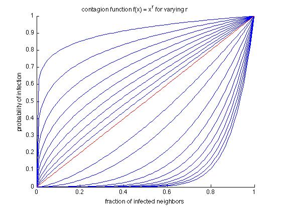
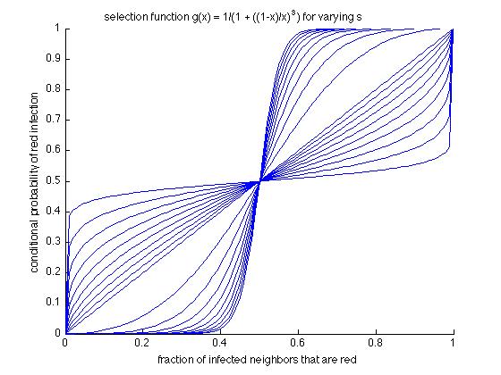
Figure 1: Left: Plots of $f(x)=x^{r}$ for varying choices of $r$, including $r=1$ (linear, red line), $r<1$ (concave), and $r>1$ (convex). Right: Plots of $g(y)=y^{s}/(y^{s}+(1-y)^{s})$ for varying choices of $s$, including $s=1$ (linear, red line), $s<1$ (equalizing), and $s>1$ (polarizing).

A fairly broad class of dynamics is captured by the following parametric family of functions. The switching function

$$f(x)=x^{r}\;\;r\geq 0$$

and the selection function

$$g(y)=y^{s}/(y^{s}+((1-y)^{s})\;\;s\geq 0.$$

Regarding this form for $f$, for $r=1$ we have linear adoption. For $r<1$ we have $f$ concave, corresponding to cases in which the probability of adoption rises quickly with only a small fraction of adopting neighbors, but then saturates or levels off with larger fractions of adopting neighbors. In contrast, for $r>1$ we have $f$ convex, which at very large values of $r$ can begin to approximate threshold adoption behavior — the probability of adoption remains small until some fraction of neighbors has adopted, then rises rapidly. See Figure 1.

Regarding this form for $g$, which is known as the Tullock contest function (Tullock (1980)), for $s=1$ we have a (linear) voter model in which the probability of selection is proportional to local market share. For $s<1$ we have what we shall call an equalizing $g$, by which we mean that selection of the minority party in the neighborhood is favored relative to the linear voter model $g(y)=y$; and for $s>1$ we have a polarizing $g$, meaning that the minority party is disfavored relative to the linear model. As $s$ approaches 0, we approach the completely equalizing choice $g\equiv 1/2$, and as $s$ approaches infinity, we approach the completely polarizing winner-take-all $g$; see Figure 1.

These parametric families of switching and selection functions will play an important role in illustrating our general results. We now discuss a few technology adoption examples which are (qualitatively) covered by these families of functions.

• Social Network Services (Facebook, Google+, etc.): Here adoption probabilities might grow slowly with a small fraction of adopting neighbors, since there is little value in using (any) social networking services if none of your friends are using them; thus a convex switching function $f$ ($r>1$) might be a reasonable model. However, given that it is currently difficult or impossible to export friends and other settings from one service to another, there are strong platform effects in service selection, so a polarizing or even winner-take-all selection function $g$ ($s>1$) might be most appropriate.

• Televisions (Sharp, Sony, etc.): Televisions were immediately useful upon their introduction, without the need for adoption by neighbors, since they allowed immediate access to broadcast programming; the adoption by neighbors serves mainly as a route for information sharing about value of the product. The information value of more neighbors adopting a product is falling with adoption and so a concave $f$ might be appropriate. Compared to social networking services, the platform effects are lower here, and so a linear or equalizing $g$ is appropriate.

• Mobile Phone Service (Verizon, T-Mobile, etc.): Mobile phone service was immediately useful upon its introduction without adoption by neighbors, since one could always call land lines, thus arguing for a concave $f$. Since telephony systems need to be interoperable, platform effects derive mainly from marketing efforts such as “Friends and Family” programs, and thus are extant but perhaps weak, suggesting an equalizing $g$.

In the proofs of some of our results, it will sometimes be convenient to use a more general adoption function formulation with some additional technical conditions that are met by our switching-selection formulation. We will refer to this general, single-step model as the generalized adoption function model. In this model, if the local fractions of Red and Blue neighbors are $\alpha_{R}$ and $\alpha_{B}$, the probability that we update the vertex with an $R$ infection is $h(\alpha_{R},\alpha_{B})$ for some adoption function $h$ with range $[0,1]$, and symmetrically the probability of $B$ infection is thus $h(\alpha_{B},\alpha_{R})$. Let us use $H(\alpha_{R},\alpha_{B})=h(\alpha_{R},\alpha_{B})+h(\alpha_{B},\alpha_{R})$ to denote the total infection probability under $h$. Note that we can still always decompose $h$ into a two-step process by defining the switching function to be $f(\alpha_{R},\alpha_{B})=H(\alpha_{R},\alpha_{B})$ and defining the selection function to be

$$g(\alpha_{R},\alpha_{B})=h(\alpha_{R},\alpha_{B})/(h(\alpha_{R},\alpha_{B})+h(\alpha_{B},\alpha_{R}))$$

which is the infection-conditional probability that $R$ wins the infection. The switching-selection model is thus the special case of the generalized adoption function model in which $H(\alpha_{R},\alpha_{B})=f(\alpha_{R}+\alpha_{B})$ is a function of only $\alpha_{R}+\alpha_{B}$, and $g(\alpha_{R},\alpha_{B})$ is a function of only $\alpha_{R}/(\alpha_{R}+\alpha_{B})$.

4 Equilibrium Examples

The examples here illustrate that our framework yields a rich class of competitive strategies, which can depend in subtle ways on the dynamics, the relative budgets of the players and the structure of the social network.

Price of Anarchy: Suppose that budgets of the firms are $K_{R}=K_{B}=1$, and the update rule is such that all vertices are updated only once. The network contains two connected components with $10$ vertices and $100$ vertices, respectively. In each component there are 2 influential vertices, each of which is connected to the other 8 and 98 vertices, respectively. So in component $1$, there are $16$ directed links while in component $2$ there are $196$ directed links in all.

• Suppose that the switching function and the selection function are both linear, $f(x)=x$ and $g(y)=y$. Then there is a unique equilibrium in which players place their seeds on distinct influential vertices of component 2. The total infection is then $100$ and this is the maximum number of infections possible with $2$ seeds. So here the PoA is $1$.

• Let us now alter the switching function such that $f(1/2)=\epsilon$ for some $\epsilon<1/2$ (keeping $f(1)=1$, as always), but retain the selection function to be $g(y)=y$. Now there also exists an equilibrium in which the firms locate on the influential vertices of component $1$. In this equilibrium payoffs to each player are equal to $5$. Observe that for $\epsilon<1/25$, a deviation to the other component is not profitable: it yields an expected payoff equal to $\epsilon\times 100$, and this is strictly smaller than $5$. Since it is still possible to infect component $2$ with $2$ seeds, the PoA is $10$. Here inefficiency is created by a coordination failure of the players.

• Finally, suppose there is only one component with $110$ vertices, with $2$ influential vertices and $108$ vertices receiving directed links. Then equilibrium under both switching functions considered above will involve firms locating at the $2$ influential vertices and this will lead to infection of all vertices. So the PoA is $1$, irrespective of whether the switching function is linear $f(x)=x$ or whether $f(1/2)<1/25$.

Thus for a fixed network, updating rule and selection function, variations in the switching function can generate large variations in the PoA. Similarly, for fixed update rule and switching and selection functions, a change in the network structure yields very different PoA.

Theorem 1 provides a set of sufficient conditions on switching and selection function, under which the PoA is uniformly bounded from above. Theorem 3 shows how even small violations of these conditions can lead to arbitrarily high PoA.

Budget Multiplier: Suppose that budgets of the firms are $K_{R}=1$, $K_{B}=2$ and the update rule is such that all vertices are updated only once. The network contains $3$ influential vertices, each of which has a directed link to all the other $n-3$ vertices, respectively. So there are $3(n-3)$ links in all. Let $n\gg 3$.

• Suppose the switching function and selection function are both linear, i.e., $f(x)=x$ and $g(y)=y$. There is a unique equilibrium and in this equilibrium, players will place their resources on distinct influential vertices. The (expected) payoffs to player $R$ are $n/3$, while the payoffs to player $B$ are $2n/3$. So the Budget Multiplier is equal to $1$.

• Next, suppose the switching function is convex with $f(2/3)=1/25$, and the selection function $g(y)$ is as in Tullock (1980). Suppose the two players place their resources on the three influential vertices. The payoffs to $R$ are $g(1/3)n$, while firm $B$ earns $g(2/3)n$. Clearly this is optimal for firm $B$ as any deviation can only lower payoffs. And, it can be checked that a deviation by firm $R$ to one of the influential vertices occupied by player $B$ will yield a payoff of $n/100$ (approximately). So the configuration specified is an equilibrium so long as $g(1/3)\geq 1/100$. The Budget Multiplier is now (approximately) 50.

• Finally, suppose the network consists of $\ell$ equally-sized connected components. In each component, there is $1$ influential vertex which has a directed link to each of the $(n/\ell)-1$ other vertices. In equilibrium each player locates on a distinct influential vertex, irrespective of whether the switching function is convex or concave and whether the Tullock selection function is linear ($s=1$) or whether it is polarizing ($s>1$). The Budget Multiplier is now equal to 1.

These examples show that for fixed network and updating rule, variations in the switching and selection functions generate large variations in Budget Multiplier. Moreover, for fixed switching and selection functions the payoffs depend crucially on the network.

Theorem 4 provides a set of sufficient conditions on the switching and selection function, under which the Budget Multiplier is uniformly bounded. Theorem 5 shows how even small violations of these conditions can lead to arbitrarily high Budget Multiplier. Theorem 6 illustrates the role of concavity of the switching function in shaping the Budget Multiplier.

5 Results: Price of Anarchy

We first state and prove a theorem providing general conditions in the switching-selection model under which the Price of Anarchy is bounded by a constant that is independent of the size and structure of the graph $G$. The simplest characterization is that $f$ being any concave function (satisfying $f(0)=0$, $f(1)=1$ and $f$ increasing), and $g$ being the linear voter function $g(y)=y$ leads to bounded PoA; but we shall see the conditions allow for certain combinations of concave $f$ and nonlinear $g$ as well. We then prove a lower bound showing that the concavity of $f$ is required for bounded PoA in a very strong sense — a small amount of convexity can lead to unbounded PoA.

5.1 PoA: Upper Bound

We find it useful to state and prove our theorems using the generalized adoption model formulation described in section 3, but with some additional conditions on $h$ that we now discuss. If $h(\alpha_{R},\alpha_{B})$ (respectively, $h(\alpha_{B},\alpha_{R})$) is the probability that a vertex with fractions $\alpha_{R}$ and $\alpha_{B}$ of $R$ and $B$ neighbors is infected by $R$ (respectively, $B$), we say that the total infection probability $H(\alpha_{R},\alpha_{B})=h(\alpha_{R},\alpha_{B})+h(\alpha_{B},\alpha_{R})$ is additive in its arguments (or simply additive) if $H$ can be written $H(\alpha_{R},\alpha_{B})=f(\alpha_{R}+\alpha_{B})$ for some increasing function $f$ — in other words, $h$ permits interpretation as a switching function. We shall say that $h$ is competitive if $h(\alpha_{R},\alpha_{B})\leq h(\alpha_{R},0)$ for all $\alpha_{R},\alpha_{B}\in[0,1]$. In other words, a player always has equal or higher infection probability in the absence of the other player.

Concave $f$ and linear $g$. Observe that the switching-selection formulation always satisfies the additivity property by definition. Moreover, in the switching-selection formulation, if $g$ is linear, the competitiveness condition becomes

$$h(x,y)=f(x+y)(x/(x+y))\leq f(x)=h(x,0)$$

or

$$f(x+y)/(x+y)\leq f(x)/x.$$

This condition is satisfied by the concavity of $f$. We will later see that the following theorem also applies to certain combinations of concave $f$ and nonlinear $g$. The first theorem can now be stated.

Theorem 1

If the adoption function $h(\alpha^{R},\alpha^{B})$ is competitive and $H$ is additive in its arguments, then Price of Anarchy is at most 4 for any graph $G$.

We establish the theorem via a series of lemmas and inequalities that can be summarized as follows. Let $(S_{R}^{*},S_{B}^{*})$ be an initial allocation of infections that gives the maximum joint payoff, and let $(S_{R},S_{B})$ be a pure Nash equilibrium with $S_{R}$ being the larger set of seeds, so $K_{R}=|S_{R}^{*}|=|S_{R}|\geq K_{B}=|S_{B}^{*}|=|S_{B}|$. We first establish a general lemma (Lemma 1) that implies that the set $S_{R}^{*}$ alone (without $S_{B}^{*}$ present) must yield payoffs close to the maximum joint payoff (Corollary 1). The proof involves the construction of a coupled stochastic process technique we employ repeatedly in the paper. We then contemplate a deviation by the Red player to $(S_{R}^{*},S_{B})$. Another coupling argument (Lemma 2) establishes that the total payoffs for both players under $(S_{R}^{*},S_{B})$ must be at least those for the Red player alone under $(S_{R}^{*},\emptyset)$. This means that under $(S_{R}^{*},S_{B})$, one of the two players must be approaching the maximum joint infections. If it is Red, we are done, since Red’s equilibrium payoff must also be this large. If it is Blue, Lemma 1 implies that Blue could still get this large payoff even after the departure of Red. Next we invoke Lemma 2 to show that total eventual payoff to both players under $(S_{R},S_{B})$ must exceed this large payoff accruing to Blue, proving the theorem.

Lemma 1

Let $A_{R}$ and $A_{B}$ be any sets of seed vertices for the two players. Then if $h$ is competitive and $H$ is additive,

$${\bf E}[\chi_{R}|(A_{R},\emptyset)]\geq{\bf E}[\chi_{R}|(A_{R},A_{B})]$$

and

$${\bf E}[\chi_{B}|(\emptyset,A_{B})]\geq{\bf E}[\chi_{B}|(A_{R},A_{B})].$$

We provide the proof for the first statement involving $\chi_{R}$; the proof for $\chi_{B}$ is identical. We introduce a simple coupled simulation technique that we shall appeal to several times throughout the paper. Consider the stochastic dynamical process on $G$ under two different initial conditions: both $A_{R}$ and $A_{B}$ are present (the joint process, denoted $(A_{R},A_{B})$ in the conditioning in the statement of the lemma); and only the set $A_{R}$ is present (the solo Red process, denoted $(A_{R},\emptyset)$). Our goal is to define a new stochastic process on $G$, called the coupled process, in which the state of each vertex $v$ will be a pair $<X_{v},Y_{v}>$. We shall arrange that $X_{v}$ faithfully represents the state of a vertex in the joint process, and $Y_{v}$ the state in the solo Red process. However, these state components will be correlated or a coupled in a deliberate manner. More precisely, we wish to arrange the coupled process to have the following properties:

1. At each step, and for any vertex state $<X_{v},Y_{v}>$, $X_{v}\in\{U,R,B\}$ and $Y_{v}\in\{U,R\}$.

2. Projecting the states of the coupled process onto either component faithfully yields the respective process. Thus, if $<X_{v},Y_{v}>$ represents the state of vertex $v$ in the coupled process, then the $\{X_{v}\}$ are stochastically identical to the joint process, and the $\{Y_{v}\}$ are stochastically identical to the solo Red process.

3. At each step, and for any vertex state $<X_{v},Y_{v}>$, $X_{v}=R$ implies $Y_{v}=R$.

Note that the first two properties are easily achieved by simply running independent joint and solo Red processes. But this will violate the third property, which yields the lemma, and thus we introduce the coupling.

For any vertex $v$, we define its initial coupled process state $<X_{v},Y_{v}>$ as follows: $X_{v}=R$ if $v\in A_{R}$, $X_{v}=B$ if $v\in A_{B}$, and $X_{v}=U$ otherwise; and $Y_{v}=R$ if $v\in A_{R}$, and $Y_{v}=U$ otherwise. It is easily verified that these initial states satisfy Properties 1 and 3 above, thus encoding the initial states of the two separate processes.

Assume for now that the first vertex or vertices $v$ to be updated in the $X$ and $Y$ processes are the same — i.e. the same vertices are updated in both the joint and solo update schedules, which may in general depend on the state of the network in each. We now describe the coupled updates of $v$. Let $\alpha^{R}_{v}$ denote the fraction of $v$’s neighbors $w$ such that $X_{w}=R$, and $\alpha^{B}_{v}$ the fraction such that $X_{w}=B$. Note that by the initialization of the coupled process, $\alpha^{R}_{v}$ is also equal to the fraction of $Y_{w}=R$ (which we denote $\tilde{\alpha}^{R}_{v}$).

In the joint process, the probability that $v$ is updated to $R$ is $h(\alpha^{R}_{v},\alpha^{B}_{v})$, and to $B$ is $h(\alpha^{B}_{v},\alpha^{R}_{v})$. In the solo Red process, the probability that $v$ is updated to $R$ is $h(\alpha^{R}_{v},0)$, which by competitiveness is greater than or equal to $h(\alpha^{R}_{v},\alpha^{B}_{v})$.

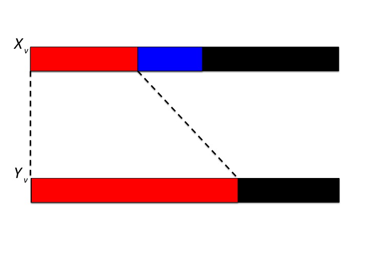
Figure 2: Illustration of the coupled dynamics defined in the proof of Lemma 1. In the update dynamic for $X_{v}$ (top line), the probabilities of Red and Blue updates are represented by disjoint line segments of length $h(\alpha^{R}_{v},\alpha^{B}_{v})$ and $h(\alpha^{B}_{v},\alpha^{R}_{v})$ respectively. By competitiveness, the Red segment has length less than $h(\alpha^{R}_{v},0)$, which is the probability of Red update of $Y_{v}$ (bottom line). The dashed red lines indicate this inequality. Thus by the arrangement of the line segments we enforce the invariant that $X_{v}=R$ implies $Y_{v}=R$.

We can thus define the update dynamics of the coupled process as follows: pick a real value $z$ uniformly at random from $[0,1]$. Update the state $<X_{v},Y_{v}>$ of $v$ as follows:

• $X_{v}$ update: If $z\in[0,h(\alpha^{R}_{v},\alpha^{B}_{v}))$, update $X_{v}$ to $R$; if $z\in[h(\alpha^{R}_{v},\alpha^{B}_{v}),h(\alpha^{R}_{v},\alpha^{B}_{v})+h(\alpha^{B}_{v},\alpha^{R}_{v})]$, update $X_{v}$ to $B$; otherwise, update $X_{v}$ to $U$. Note that the probabilities $X_{v}$ are updated to $R$ and $B$ exactly match those of the joint process, as required by Property 2 above. See Figure 2.

• $Y_{v}$ update: If $z\in[0,h(\alpha^{R}_{v},0)]$, update $Y_{v}$ to $R$; otherwise, update $Y_{v}$ to $U$. The probability $Y_{v}$ is updated to $R$ is thus exactly $h(\alpha^{R}_{v},0)$, matching that in a solo Red process. See Figure 2.

Since by competitiveness, $z\in[0,h(\alpha^{R}_{v},\alpha^{B}_{v}))$ implies $z\in[0,h^{R}(\alpha^{R}_{v},0)]$, we ensure Property 3. Thus in subsequent updates we shall have $\alpha^{R}\leq\tilde{\alpha}^{R}$. Thus as long as $h(\alpha^{R},\alpha^{B})\leq h(\tilde{\alpha}^{R},0)$ we can continue to maintain the invariant. These inequalities follow from competitiveness and the additivity of $H$.

So far we have assumed the same vertices were candidates for updating in both the joint and solo processes; while this may be true for some update schedules, in general it will not be (such as in parallel updates of all uninfected vertices, where vertices with only blue neighbors in the joint process will not be candidates for updating in the red solo process). However, this is easily handled by considering three cases. Case 1: Assuming Property 3 holds, if a vertex is a candidate for updating in both processes, we can maintain this property by performing the coupled updates described above. Case 2: If a vertex $v$ is a candidate for updating only in the solo red process, then by Property 3 $X_{v}$ cannot be $R$, so Property 3 will still hold after the update of $Y_{v}$. Case 3: Finally, if $v$ is a candidate for updating only in the joint process, then if $Y_{v}=R$, Property 3 will still hold after the update of $X_{v}$, and if $Y_{v}=U$ and all neighbors of $v$ in the joint process are $B$, Property 3 will remain true after the update. The only case remaining is that $Y_{v}=U$ and $v$ has $R$ neighbors in the joint process. This is impossible for the update schedules mentioned in Section 2.2: $v$ should have also been a candidate for updating in the solo red process, since by Property 3 $v$ has weakly more $R$ neighbors in the solo process.

Since Properties 2 and 3 hold on an update-by-update basis in any run or sample path of the coupled dynamics, they also hold in expectation over runs, yielding the statement of the lemma.  (Lemma 1)

Corollary 1

Let $A_{R}$ and $A_{B}$ be any sets of seeded nodes for the two players. Then if the adoption function $h(\alpha^{R},\alpha^{B})$ is competitive and $H$ is additive,

$${\bf E}[\chi_{R}+\chi_{B}|(A_{R},A_{B})]\leq{\bf E}[\chi_{R}|(A_{R},\emptyset)]+{\bf E}[\chi_{B}|(\emptyset,A_{B})].$$

Follows from linearity of expectation applied to the left hand side of the inequality, and two applications of Lemma 1.  (Corollary 1)

Let $(S_{R}^{*},S_{B}^{*})$ be the maximum joint payoff seed sets. Let $(S_{R},S_{B})$ be any (pure) Nash equilibrium, with $S_{R}$ having the larger budget. Corollary 1 implies either ${\bf E}[\chi_{R}|(S_{R}^{*},\emptyset)]$ or ${\bf E}[\chi_{B}|(\emptyset,S_{B}^{*})]$ is at least as great as ${\bf E}[\chi_{R}+\chi_{B}|(S_{R}^{*},S_{B}^{*})]/2$; so assume without loss of generality that ${\bf E}[\chi_{R}|(S_{R}^{*},\emptyset)]\geq{\bf E}[\chi_{R}+\chi_{B}|(S_{R}^{*},S_{B}^{*})]/2$. Let us now contemplate a unilateral deviation of the Red player from $S_{R}$ to $S_{R}^{*}$, in which case the strategies are $(S_{R}^{*},S_{B})$. In the following lemma we show that total number of eventual adoptions for the two players is larger than adoptions accruing to a single player under solo seeding.

Lemma 2

Let $A_{R}$ and $A_{B}$ be any sets of seeded nodes for the two players. If $H$ is additive,

$${\bf E}[\chi_{R}+\chi_{B}|(A_{R},A_{B})]\geq{\bf E}[\chi_{R}|(A_{R},\emptyset)].$$

We employ a coupling argument similar to that in the proof of Lemma 1. We define a stochastic process in which the state of a vertex $v$ is a pair $<X_{v},Y_{v}>$ in which the following properties are obeyed:

1. At each step, and for any vertex state $<X_{v},Y_{v}>$, $X_{v}\in\{R,B,U\}$ and $Y_{v}\in\{R,U\}$.

2. Projecting the state of the coupled process onto either component faithfully yields the respective process. Thus, if $<X_{v},Y_{v}>$ represents the state of vertex $v$ in the coupled process, then the $\{X_{v}\}$ are stochastically identical to the joint process $(A_{R},A_{B})$, and the $\{Y_{v}\}$ are stochastically identical to the solo Red process $(A_{R},\emptyset)$.

3. At each step, and for any vertex state $<X_{v},Y_{v}>$, $Y_{v}=R$ implies $X_{v}=R$ or $X_{v}=B$.

We initialize the coupled process in the obvious way: if $v\in A_{R}$ then $X_{v}=R$, if $v\in A_{B}$ then $X_{v}=B$, and $X_{v}=U$ otherwise; and if $v\in A_{R}$ then $Y_{v}=R$, and $Y_{v}=U$ otherwise. Let us fix a vertex $v$ to update, and let $\alpha^{R}_{v},\alpha^{B}_{v}$ denote the fraction of neighbors $w$ of $v$ with $X_{w}=R$ and $X_{w}=B$ respectively, and let $\tilde{\alpha}^{R}_{v}$ denote the fraction with $Y_{w}=R$. Initially we have $\alpha^{R}_{v}=\tilde{\alpha}^{R}_{v}$.

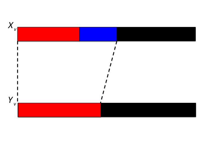
Figure 3: Illustration of the coupled dynamics defined in the proof of Lemma 2. In the update dynamic for $X_{v}$ (top line), the probabilities of Red and Blue updates are represented by line segments of length $h(\alpha^{R}_{v},\alpha^{B}_{v})$ and $h(\alpha^{B}_{v},\alpha^{R}_{v})$ respectively. By additivity of $H$, together these two segments are greater than $h(\alpha^{R}_{v},0)$ which is the probability of Red update of $Y_{v}$ (bottom line). This inequality is represented by the dashed black lines.

We assume the vertex or vertices $v$ to be updated in the $X$ and $Y$ processes are the same; the fact that the update schedules may cause these sets to differ is handled in the same way as in the proof of Lemma 1. On the first update of $v$ in the joint process $(A_{R},A_{B})$, the total probability infection by either $R$ or $B$ is

$$H(\alpha^{R}_{v},\alpha^{B}_{v})=h(\alpha^{R}_{v},\alpha^{B}_{v})+h(\alpha^{B}_{v},\alpha^{R}_{v}).$$

In the solo process $(A_{R},\emptyset)$, the probability of infection by $R$ is $h(\alpha^{R}_{v},0)\leq h(\alpha^{R}_{v},0)+h(0,\alpha^{R}_{v})=H(\alpha^{R}_{v},0)\leq H(\alpha^{R}_{v},\alpha^{B}_{v})$ where the last inequality follows by the additivity of $H$.

We thus define the update dynamics in the coupled process as follows: pick a real value $z$ uniformly at random from $[0,1]$. Update $<X_{v},Y_{v}>$ as follows:

• $X_{v}$ update:
  If $z\in[0,h(\alpha^{R}_{v},\alpha^{B}_{v}))$, update $X_{v}$ to $R$;
  if $z\in[h(\alpha^{R}_{v},\alpha^{B}_{v}),h(\alpha^{R}_{v},\alpha^{B}_{v})+h(\alpha^{B}_{v},\alpha^{R}_{v})]\\ \equiv[h(\alpha^{R}_{v},\alpha^{B}_{v}),H(\alpha^{R}_{v},\alpha^{B}_{v})]$, update $X_{v}$ to $B$;
  otherwise update $X_{v}$ to $U$. See Figure 3.

• $Y_{v}$ update: If $r\in[0,h(\alpha^{R}_{v},0))$, update $Y_{v}$ to $R$;
  otherwise update $Y_{v}$ to $U$. See Figure 3.

It is easily verified that at each such update, the probabilities of $R$ and $B$ updates of $X_{v}$ are exactly as in the joint $(A_{R},A_{B})$ process, and the probability of an $R$ update of $Y_{v}$ is exactly as in the solo $(A_{R},\emptyset)$ process, thus maintaining Property 2 above. Property 3 follows from the previously established fact that $h(\alpha^{R}_{v},0)\leq H(\alpha^{R}_{v},\alpha^{B}_{v})$, so whenever $Y_{v}$ is updated to $R$, $X_{v}$ is updated to either $R$ or $B$.

Notice that since $h(\alpha^{R}_{v},0)\geq h(\alpha^{R}_{v},\alpha^{B}_{v})$ by competitiveness, for the overall theorem (which requires competitiveness of $h$) we cannot ensure that $Y_{v}=R$ is always accompanied by $X_{v}=R$. Thus the Red infections in the solo process may exceed those in the joint process, yielding $\tilde{\alpha}^{R}_{v}>\alpha^{R}_{v}$ for subsequent updates. To maintain Property 3 in subsequent updates we thus require that $\tilde{\alpha}^{R}_{v}\leq\alpha^{R}_{v}+\alpha^{B}_{v}$ implies $h(\tilde{\alpha}^{R}_{v},0)\leq H(\tilde{\alpha}^{R}_{v},0)\leq H(\alpha^{R}_{v},\alpha^{B}_{v})$ which follows from the additivity of $H$. Also, notice that since the lemma holds for every fixed $A_{R}$ and $A_{B}$, it also holds in expectation for mixed strategies.  (Lemma 2)

Continuing the analysis of a unilateral deviation by the Red player from $S_{R}$ to $S_{R}^{*}$, we have thus established

$${\bf E}[\chi_{R}+\chi_{B}|(S_{R}^{*},S_{B})]$$

$$= {\bf E}[\chi_{R}|(S_{R}^{*},S_{B})]+{\bf E}[\chi_{B}|(S_{R}^{*},S_{B})]$$

$$\geq {\bf E}[\chi_{R}|(S_{R}^{*},\emptyset)]$$

$$\geq {\bf E}[\chi_{R}+\chi_{B}|(S_{R}^{*},S_{B}^{*})]/2$$

where the equality is by linearity of expectation, the first inequality follows from Lemma 2, and the second inequality from Corollary 1. Thus at least one of ${\bf E}[\chi_{R}|(S_{R}^{*},S_{B})]$ and ${\bf E}[\chi_{B}|(S_{R}^{*},S_{B})]$ must be at least ${\bf E}[\chi_{R}+\chi_{B}|(S_{R}^{*},S_{B}^{*})]/4$.

If ${\bf E}[\chi_{R}|(S_{R}^{*},S_{B})]\geq{\bf E}[\chi_{R}+\chi_{B}|(R^{*},B^{*})]/4$, then since $(S_{R},S_{B})$ is Nash, ${\bf E}[\chi_{R}|(S_{R},S_{B})]\geq{\bf E}[\chi_{R}+\chi_{B}|(S_{R}^{*},S_{B}^{*})]/4$, and the theorem is proved. The only remaining case is where ${\bf E}[\chi_{B}|(S_{R}^{*},S_{B})]\geq{\bf E}[\chi_{R}+\chi_{B}|(S_{R}^{*},S_{B}^{*})]/4$. But Lemma 1 has already established that ${\bf E}[\chi_{B}|(\emptyset,S_{B})]\geq{\bf E}[\chi_{B}|(S_{R}^{*},S_{B})]$, and we have ${\bf E}[\chi_{R}+\chi_{B}|(S_{R},S_{B})]\geq{\bf E}[\chi_{B}|(\emptyset,S_{B})]$ from Lemma 2. Combining, we have the following chain of inequalities:

$${\bf E}[\chi_{R}+\chi_{B}|(S_{R},S_{B})] \geq {\bf E}[\chi_{B}|(\emptyset,S_{B})]$$

$$\geq {\bf E}[\chi_{B}|(S_{R}^{*},S_{B})]$$

$$\geq {\bf E}[\chi_{R}+\chi_{B}|(S_{R}^{*},S_{B}^{*})]/4$$

thus establishing the theorem.  (Theorem 1)

Concave $f$, non-linear $g$. Recall that the switching-selection formulation in which $f$ is concave and $g$ is linear satisfies the hypothesis of the Theorem above. But Theorem 1 also provides more general conditions for bounded PoA in the switching-selection model. For example, suppose we consider switching functions of the form $f(x)=x^{r}$ for $r\leq 1$ (thus yielding concavity) and selection functions of the Tullock contest form $g(y)=y^{s}/(y^{s}+(1-y)^{s})$, as discussed in Section 2.2. Letting $a$ and $b$ denote the local fraction of Red and Blue neighbors for notational convenience, this leads to an adoption function of the form $h(a,b)=(a+b)^{r}/(1+(b/a)^{s})$. The condition for competitiveness is

$$h(a,0)-h(a,b)=a^{r}-(a+b)^{r}/(1+(b/a)^{s})\geq 0.$$

Dividing through by $(a+b)^{r}$ yields

$$(a/(a+b))^{r}-1/(1+(b/a)^{s})$$

$$=1/(1+(b/a))^{r}-1/(1+(b/a)^{s})\geq 0.$$

Making the substitution $z=b/a$ and moving the second term to the right-hand side gives

$$1/(1+z)^{r}\geq 1/(1+z^{s}).$$

Thus competitiveness is equivalent to the condition $1+z^{s}\geq(1+z)^{r}$ for all $z\geq 0$. It is not difficult to show that any $s\in[r,1]$ will satisfy this condition. In other words, the more concave $f$ is (i.e. the smaller $r$ is), the more equalizing $g$ can be (i.e. the smaller $s$ can be) while maintaining competitiveness. By Theorem 1 we have thus shown:

Corollary 2

Let the switching function be $f(x)=x^{r}$ for $r\leq 1$ and let $g(y)=y^{s}/(y^{s}+(1-y)^{s})$ be the selection function. Then as long as $s\in[r,1]$, the Price of Anarchy is at most 4 for any graph.

5.2 PoA: Lower Bound

We now show that concavity of the switching function is required in a very strong sense — essentially, even a slight convexity leads to unbounded PoA. As a first step in this demonstration, it is useful to begin with a simpler result showing that the PoA is unbounded if the switching function is permitted to violate concavity to an arbitrary extent.

Theorem 2

Fix $\alpha^{*}\in(0,1)$, and let the switching function $f$ be the threshold function $f(x)=0$ for $x<\alpha^{*}$, and $f(x)=1$ for $x\geq\alpha^{*}$. Let the selection function be linear $g(y)=y$. Then for any value $V>0$, there exists $G$ such that the Price of Anarchy in $G$ is greater than $V$.

Let $m$ be a large integer, and set the initial budgets of both players to be $\alpha^{*}m/2$. The graph $G$ will consist of two components. The first component $C_{1}$ consists of two layers; the first layer has $m$ vertices and the second $n_{1}$ vertices, and there is a directed edge from every vertex in the first layer to every vertex in the second layer. The second component $C_{2}$ has the same structure, but with $m$ vertices in the first layer and $n_{2}$ in the second layer. We let $n_{2}\gg n_{1}\gg m$. For concreteness, let us choose an update schedule that updates each vertex in the second layers of the two components exactly once in some fixed ordering (the same result holds for many other updating schedules).

It is easy to see that the maximum joint profit solution is to place the combined $\alpha^{*}m$ of seeds of the two players in the first layer $C_{2}$, in which case the number of second-layer infections will be $n_{2}$ since $f(\alpha^{*})=1$. Any configuration which places at least one infection in each of the two components will not cause any second-layer infections, since then the threshold of $f$ will not be exceeding in either component.

It is also easy to see that both players placing all their infections in the first layer of $C_{1}$, which will result in $n_{1}$ infections in the second layer since the threshold is exceeded, is a Nash equilibrium. Any deviation of a player to $C_{2}$, or to layer 2 of $C_{1}$, causes the threshold to no longer be exceeded in either component. Thus the PoA here is $n_{2}/n_{1}$, which can be made arbitrarily large. Note that the maximum joint infections solution is also a Nash equilibrium — we are exploiting the worst-case (over Nash) nature of the PoA here (as will all our lower bounds, though see Footnote 5).  (Theorem 2)

Thus, a switching function strongly violating concavity can lead to unbounded PoA even with a linear selection function. But it turns out that functions even slightly violating concavity also cause unbounded PoA — as we shall see, network structure can amplify small amounts of convexity.

Theorem 3

Let the switching function be $f(x)=x^{r}$ for any $r>1$, and let the selection function be linear $g(y)=y$. Then for any $V>0$, there exists a graph $G$ for which the Price of Anarchy is greater than $V$. More precisely, there is a family of graphs for which the Price of Anarchy grows linearly with the population size (number of vertices).

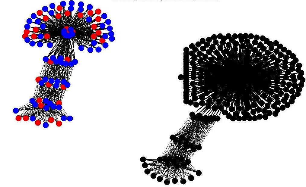
Figure 4: Illustration of convexity amplification in the Price of Anarchy lower bound of Theorem 3, under convex switching function $f(x)=x^{3}$ and linear selection function $g$. Top: Two-component, directed, layered “flower” graph, with the right flower having many more petals than the left. In the configuration shown, both players play in the first layer of the stem of the smaller flower. The convexity of $f$ does not enter the dynamics, since at each update an entire successive layer is infected, quickly reaching the petals. Bottom: However, if the two players locate in different components, layers are not fully infected and the convexity of $f$ is amplified via composition in successive layers, damping out the infection rate quickly.

The idea is to create a layered, directed graph whose dynamics rapidly amplify the convexity of $f$. Taking two such amplification components of differing sizes yields an equilibrium in which the players coordinate on the smaller component, while the maximum joint payoffs solution lies in the larger component. The construction of the proof is illustrated in Figure 4.

The amplification gadget will be a layered, directed graph with $\ell_{i}$ vertices in the $i$th layer and $N$ layers total. There are directed edges from every vertex in layer $i$ to every vertex in layer $i+1$, and no other edges. Let the two players have equal budgets of $k$, and define $\alpha=2k/\ell_{1}$ — thus, $\alpha$ is the fraction of layer 1 the two players could jointly infect.

Let us consider what happens if indeed the two players jointly infect $2k$ vertices in the first layer, and the update schedule proceeds by updating each successive layer $2,\ldots,N$. Since every vertex in layer 2 has every vertex in layer 1 as a directed neighbor, and no others, the expected fraction of layer 2 that is infected is $f(\alpha)=\alpha^{r}$. Inductively, the expected fraction of layer 3 that is infected is thus $f(f(\alpha))=\alpha^{r^{2}}$. In general, the expected fraction of layer $i$ that is infected is $\alpha^{r^{i-1}}$, and by the linearity of $g$ the two players will split these infections. Here, we note that the actual path of infections will be stochastic; this stochastic path is well approximated by the expected infections, if layers are sufficiently large. Throughout this proof we will use this approximation (which relies on an appeal to the strong law of large numbers).

Now let $\alpha=\beta_{1}+\beta_{2}$, and let us instead place $\beta_{1}\ell_{1}$ seeds at layer 1 and $\beta_{2}\ell_{1}$ at layer $i$. The total number of infections expected at layer $i$ now becomes $\beta_{1}^{r^{i-1}}\ell_{i}+\beta_{2}\ell_{1}$. By the convexity of the function $f^{(i-1)}(x)=x^{r^{i-1}}$, this will be smaller than $\alpha^{r^{i-1}}\ell_{i}=(\beta_{1}+\beta_{2})^{r^{i-1}}\ell_{i}$ as long as $\beta_{2}\ell_{1}<\beta_{2}^{r^{i-1}}\ell_{i}$, or $\ell_{i}>\ell_{1}/\beta_{2}^{r^{i-2}}$. Also, notice that the smallest nonzero deviation requires $\beta_{2}\ell_{1}\geq 1$, or $\beta_{2}\geq 1/\ell_{1}$. Thus as long as $\ell_{i}\geq\ell_{1}^{r^{i-1}}$, the total fraction of infections generated by placing $\beta_{1}\ell_{1}$ seeds at layer 1 and $\beta_{2}\ell_{1}$ at layer $i$ will be less than by placing all in layer 1. Furthermore, by the linearity of $g$, any individual player who effects such a unilateral deviation will suffer.

Note that we can make the final, $N$th, layer arbitrarily large. In particular, if we choose $\ell_{i}=\ell_{1}^{r^{i-1}}$ as specified above for all $2\leq i\leq N-1$, and choose $\alpha^{r^{N-1}}\ell_{N}\gg\sum_{i=1}^{N-1}\alpha^{r^{i-1}}\ell_{i}$, the total expected number of infections conditioned on both players playing in the first layer will be dominated by the $\alpha^{r^{N-1}}\ell_{N}$ expected infections in the final layer.

Now consider a graph consisting of two disjoint amplification gadgets $G_{1}$ and $G_{2}$ that are exactly as described above, but differ only in the sizes of their final $N$th layers — $\ell_{N}(1)$ for $G_{1}$ and $\ell_{N}(2)$ for $G_{2}$, where we will choose $\ell_{N}(2)\gg\ell_{N}(1)$. Consider a configuration where all seeds are in the first layer of $G_{1}$. We have already argued above that no deviation to later layers of $G_{1}$ can be profitable. Now let us consider a unilateral deviation of the Red player from $G_{1}$ to the first layer of $G_{2}$. Since Red alone infects now only infects a fraction $\alpha/2$ of the $\ell_{1}$ vertices in the first layer of $G_{2}$, the expected final number of Red infections will be approximately $(\alpha/2)^{r^{N-1}}\ell_{N}(2)$, compared with $\alpha^{r^{N-1}}\ell_{N}(1)/2$ for not deviating from $G_{1}$. Thus as long as $(\alpha/2)^{r^{N-1}}\ell_{N}(2)\leq\alpha^{r^{N-1}}\ell_{N}(1)/2$, or $\ell_{N}(2)/\ell_{N}(1)\leq 2^{r^{N-1}-1}$, this deviation is unprofitable for Red. More generally, if Red divides its $(\alpha/2)\ell_{1}$ resources by placing a fraction $\beta_{1}$ of them in the first layer of $G_{1}$ and a fraction $\beta_{2}=1-\beta$ of them in the first layer of $G_{2}$, its expected payoff is

$$\left[(1+\beta_{1})(\alpha/2)\right]^{r^{N-1}}\ell_{N}(1)\frac{\beta_{1}}{1+\beta_{1}}+\left[\beta_{2}(\alpha/2)\right]^{r^{N-1}}\ell_{N}(2).$$

The first term of this sum represents the share of the final layer of $G_{1}$ that Red obtains given that Blue is playing entirely in this component, while the second term represents the uncontested infections Red wins in $G_{2}$. This expression can be written as

$$\alpha^{r^{N-1}}\left[\left(\frac{1+\beta_{1}}{2}\right)^{r^{N-1}}\ell_{N}(1)\frac{\beta_{1}}{1+\beta_{1}}+\left(\frac{1-\beta_{1}}{2}\right)^{r^{N-1}}\ell_{N}(2)\right]$$

which for the choice $\ell_{N}(2)=2^{r^{N-1}}\ell_{N}(1)/2$ becomes

$$\alpha^{r^{N-1}}\left[\left(\frac{1+\beta_{1}}{2}\right)^{r^{N-1}}\ell_{N}(1)\frac{\beta_{1}}{1+\beta_{1}}+\left({1-\beta_{1}}\right)^{r^{N-1}}\ell_{N}(1)/2\right].$$

For any $0<\beta_{1}<1$, both terms inside the brackets above are exponentially damped and result in suboptimal payoff for Red. Thus the best response choices are given by the extremes $\beta_{1}=1$ and $\beta_{1}=0$, which both yield expected payoff $\ell_{N}(1)/2$ for Red. (Note that by choosing $\ell_{N}(2)$ slightly smaller above, we can force $\beta_{1}=1$ to be a strict best response.)

However, the maximum joint payoffs solution (as well as the best, as opposed to worst Nash equilibrium) is for both players to initially infect in the first layer of $G_{2}$, in which case the total payoff will be approximately $\alpha^{r^{N-1}}\ell_{N}(2)$. The Price of Anarchy is thus

$$\frac{\alpha^{r^{N-1}}\ell_{N}(2)}{\alpha^{r^{N-1}}\ell_{N}(1)}=\frac{\ell_{N}(2)}{\ell_{N}(1)}\geq 2^{r^{N-1}-1}$$

by the choice of $\ell_{N}(2)$ above. Thus by choosing the number of layers $N$ as large as needed, the Price of Anarchy exceeds any finite bound $V$.  (Theorem 3)

Combining Theorem 1 and Theorem 3, we note that for $f(x)=x^{r}$ and linear $g$ we obtain the following sharp threshold result:

Corollary 3

Let the switching function be $f(x)=x^{r}$, and let the selection function be linear, $g(y)=y$. Then:

• For any $r\leq 1$, the Price of Anarchy is at most 4 for any graph $G$;

• For any $r>1$ and any $V$, there exists a graph $G$ for which the Price of Anarchy is greater than $V$.

6 Results: Budget Multiplier

We derive sufficient conditions for bounded Budget Multiplier, and show that violations of these conditions can lead to unbounded Budget Multiplier.

6.1 Budget Multiplier: Upper Bound

As in the PoA analysis, it will be technically convenient to return to the generalized adoption function model. Recall that for PoA, competitiveness of $h$ and additivity of $H$ were needed to prove upper bounds, but we didn’t require that the implied selection function be linear. Here we introduce that additional requirement, and prove that the (pure strategy) Budget Multiplier is bounded.

Theorem 4

Suppose the adoption functions $h(\alpha^{R},\alpha^{B})$ is competitive, that $H$ is additive in its arguments, and that the implied selection function is linear:

$$g(\alpha_{R},\alpha_{B})=\frac{h(\alpha_{R},\alpha_{B})}{h(\alpha_{R},\alpha_{B})+h(\alpha_{B},\alpha_{B})}=\alpha_{R}/(\alpha_{R}+\alpha_{B})$$

Then the pure strategy Budget Multiplier is at most 2 for any graph $G$.

The proof borrows elements from the proof of Theorem 1, and introduces the additional notion of tracking or attributing indirect infections generated by the dynamics to specific seeds.

Consider any pure Nash equilibrium given by seed sets $S_{R}$ and $S_{B}$ in which $|S_{R}|=K>|S_{B}|=L$. For our purposes the interesting case is one in which

$${\bf E}[\chi_{R}|(S_{R},S_{B})]\geq{\bf E}[\chi_{B}|(S_{R},S_{B}))]$$

and so

$${\bf E}[\chi_{R}|(S_{R},S_{B})]\geq{\bf E}[\chi_{R}+\chi_{B}|(S_{R},S_{B})]/2.$$

Since the adoption function is competitive and additive, Lemma 1 implies that ${\bf E}[\chi_{R}|(S_{R},\emptyset)]\geq E[\chi_{R}|(S_{R},S_{B})]$ — that is, the Red player only benefits from the departure of the Blue player.

Let us consider the dynamics of the solo Red process given by $(S_{R},\emptyset)$. We first introduce a faithful simulation of these dynamics that also allows us to attribute subsequent infections to exactly one of the seeds in $S_{R}$; we shall call this process the attribution simulation of $(S_{R},\emptyset)$. Thus, let $S_{R}=\{v_{1},\ldots,v_{K}\}$ be the initial Red infections, and let us label $v_{i}$ by $R_{i}$, and label all other vertices $U$. All infections in the process will also be assigned one of the $K$ labels $R_{i}$ in the following manner: when updating a vertex $v$, we first compute the fraction $\alpha^{R}_{v}$ of neighbors whose current label is one of $R_{1},\ldots,R_{K}$, and with probability $H(\alpha^{R}_{v},0)=h(\alpha^{R}_{v},0)+h(0,\alpha^{R}_{v})$ we decide that an infection will occur (otherwise the label of $v$ is updated to $U$). If an infection occurs, we simply choose an infected neighbor of $v$ uniformly at random, and update $v$ to have the same label (which will be one of the $R_{i}$). It is easily seen that at every step, the dynamics of the $(S_{R},\emptyset)$ process are faithfully implemented if we drop label subscripts and simply view any label $R_{i}$ as a generic Red infection $R$. Furthermore, at all times every infected vertex has only one of the labels $R_{i}$. Thus if we denote the expected number of vertices with label $R_{i}$ by ${\bf E}[\chi_{R_{i}}|(S_{R},\emptyset)]$, we have ${\bf E}[\chi_{R}|(S_{R},\emptyset)]=\sum_{i=1}^{K}{\bf E}[\chi_{R_{i}}|(S_{R},\emptyset)]$. Let us assume without loss of generality that the labels $R_{i}$ are sorted in order of decreasing ${\bf E}[\chi_{R_{i}}|(S_{R},\emptyset)]$.

We now consider the payoff to Blue under a deviation from $S_{B}$ to the set $\hat{S}_{B}=\{v_{1},\ldots,v_{L}\}\subset S_{R}$ — that is, the $L$ “most profitable” initial infections in $S_{R}$. Our goal is to show that the Blue player must enjoy roughly the same payoff from these $L$ seeds as the Red player did in the solo attribution simulation.

Lemma 3

$${\bf E}[\chi_{B}|(S_{R},\hat{S}_{B})] \geq \frac{1}{2}\sum_{i=1}^{L}{\bf E}[\chi_{R_{i}}|(S_{R},\emptyset)]$$

$$\geq \frac{L}{2K}{\bf E}[\chi_{R}|(S_{R},\emptyset)]$$

The second inequality follows from

$${\bf E}[\chi_{R}|(S_{R},\emptyset)]=\sum_{i=1}^{K}{\bf E}[\chi_{R_{i}}|(S_{R},\emptyset)],$$

established above, and fact that the vertices in $S_{R}$ are ordered in decreasing profitability. For the first inequality, we introduce coupled attribution simulations for the two processes $(S_{R},\emptyset)$ (the solo Red process) and $(S_{R},\hat{S}_{B})$. For simplicity, let us actually examine $(S_{R},\emptyset)$ and $(S_{R}-\hat{S}_{B},\hat{S}_{B})$; the latter joint process is simply the process $(S_{R},\hat{S}_{B})$, but in which the contested seeded nodes in $\hat{S}_{B}$ are all won by the Blue player. (The proof for the general $(S_{R},\hat{S}_{B})$ case is the same but causes the factor of $1/2$ in the lemma.)

The coupled attribution dynamics are as follows: as above, in the solo Red process, for $1\leq i\leq L$, the vertex $v_{i}$ in $S_{R}$ is initially labeled $R_{i}$, and all other vertices are labeled $U$. In the joint process, the vertex $v_{i}$ is labeled $B_{i}$ for $i\leq L$ (corresponding to the Blue invasions of $S_{R}$), while for $L<i\leq K$ the vertex $v_{i}$ is labeled $R_{i}$ as before. Now at the first update vertex $v$, let $\alpha^{R}_{v}$ be the fraction of Red neighbors in the solo process, and let $\tilde{\alpha}^{R}_{v}$ and $\tilde{\alpha}^{B}_{v}$ be the fraction of Red and Blue neighbors, respectively, in the joint process.

Note that initially we have $\alpha^{R}_{v}=\tilde{\alpha}^{R}_{v}+\tilde{\alpha}^{B}_{v}$. Thus by additivity $H$, the total probabilities of infection $H(\alpha^{R}_{v},0)$ and $H(\tilde{\alpha}^{R}_{v},\tilde{\alpha}^{B}_{v})$ in the two processes must be identical. We thus flip a common coin with this shared infection probability to determine whether infections occur in the coupled process. If not, $v$ is updated to $U$ in both processes. If so, we now use a coupled attribution step in which we pick an infected neighbor of $v$ at random and copy its label to $v$ in both processes. Thus if a label with index $i\leq L$ is chosen, $v$ will be updated to $R_{i}$ in the solo process, and to $B_{i}$ in the joint process; whereas if $L<i\leq K$ is chosen, the update will be to $R_{i}$ in both processes. It is easily verified that each of the two processes faithfully implement the dynamics of the solo and joint attribution processes, respectively.

This coupled update dynamic maintains two invariants: infections are always matched in the two processes, thus maintaining $\alpha^{R}_{v}=\tilde{\alpha}^{R}_{v}+\tilde{\alpha}^{B}_{v}$ for all $v$ and every step; and for all $i\leq L$, every $R_{i}$ attribution in the solo Red process is matched by a $B_{i}$ attribution in the joint process, thus establishing the lemma.  (Lemma 3)

Thus, by simply imitating the strategy of the Red player in the $L$ most profitable resources, the Blue player can expect to infect $(1/2)(L/K)$ proportion of infections accruing to Red in isolation. Since $(S_{R},S_{B})$ is an equilibrium, the payoffs of Blue in equilibrium must also respect this inequality.  (Theorem 4)

6.2 Budget Multiplier: Lower Bound

We have already seen that concavity of $f$ and linearity of $g$ lead to bounded PoA and Budget Multiplier, and that even slight deviations from concavity can lead to unbounded PoA. We now show that fixing $f$ to be linear (which is concave), slight deviations from linearity of $g$ towards polarizing $g$ can lead to unbounded Budget Multiplier, for similar reasons as in the PoA case: graph structure can amplify a slightly polarizing $g$ towards arbitrarily high punishment of the minority player.

Theorem 5

Let the switching function be $f(x)=x$, and let the selection function be of Tullock contest form, $g(y)=y^{s}/(y^{s}+((1-y)^{s})$, where $s>1$. Then for any $V>0$, there exists a graph $G$ for which the Budget Multiplier is greater than $V$. More precisely, there is a family of graphs for which the Budget Multiplier grows linearly with the population size (number of vertices).

As in the PoA lower bound, the proof relies on a layered amplification graph, this time amplifying punishment in the selection function rather than convexity in the switching function. The graph will consist of two components, $C_{1}$ and $C_{2}$.

Let us fix the budget of the Red player to be 3, and that of the Blue player to be 1 (the proof generalizes to other unequal values). $C_{1}$ is a directed, layered graph with $k+1$ layers. The first layer has $4$ vertices, and layers 2 through $k$ have $n\gg 4$ vertices, while layer $k+1$ has $n_{1}$ vertices, where we shall choose $n_{1}\gg n$, meaning that payoffs in $C_{1}$ are dominated by infections in the final layer.

The second component $C_{2}$ is a 2-layer directed graph, with 1 vertex in the first layer and $n_{2}$ in the final layer, and all directed edges from layer 1 to 2. We will eventually choose $n_{2}\ll n_{1}$, so that $C_{1}$ is the much bigger component. We choose an update rule in which each layer is updated in succession and only once.

Consider the configuration in which Red places its 3 infections in the first layer of $C_{1}$, and Blue places its 1 infection in the first layer of $C_{2}$. We shall later show that this configuration is a Nash equilibrium. In this configuration, the expected payoff to Red is approximately $\sum_{i=2}^{k}(3/4)n+(3/4)n_{1}$ by linearity of $f$; notice that the selection function does not enter since the players are in disjoint components. Similarly, the expected payoff to Blue is $n_{2}$. In this configuration, the ratio of Red and Blue expected payoffs is thus at least $(3/4)n_{1}/n_{2}$, whereas the initial budget ratio is $1/3$. So the Budget Multiplier for this configuration is at least $n_{1}/(4n_{2})$.

We now develop conditions under which this configuration is an equilibrium. It is easy to verify that red is playing a best response. Moving vertices to later layers of $C_{1}$ lowers Red’s payoff, since $n\gg 4$ and $f$ is linear. Finally, moving infections to invade the first layer of $C_{2}$ will lower Red’s payoff as long as, say, $(1/4)n_{1}$ (Red’s current payoff per initial infection in the final layer of $C_{1}$) exceeds $n_{2}$ (the maximum amount Red could get in $C_{2}$ by full deviation), or $n_{1}\gg 4n_{2}$.

We now turn to deviations by Blue. Moving the solo Blue initial infection to the second layer of $C_{2}$ is clearly a losing proposition. So consider deviations in which Blue moves to vertices in component 1. If he moves to the lone unoccupied vertex in layer 1 of $C_{1}$, his payoff is approximately:

$$\sum_{i=2}^{k}g^{(i)}(1/4)n+g^{(k+1)}(1/4)n_{1}$$

$$= \sum_{i=2}^{k}\frac{(1/4)^{s^{i}}}{(1/4)^{s^{i}}+(3/4)^{s^{i}}}n$$

$$+\frac{(1/4)^{s^{k+1}}}{(1/4)^{s^{k+1}}+(3/4)^{s^{k+1}}}n_{1}$$

Similarly, if Blue directly invades a Red vertex, Blue’s payoff is approximately

$$\chi=\sum_{i=2}^{k}\frac{(1/3)^{s^{i}}}{(1/3)^{s^{i}}+(2/3)^{s^{i}}}n+\frac{(1/3)^{s^{k+1}}}{(1/3)^{s^{k+1}}+(2/3)^{s^{k+1}}}n_{1}$$

Since in both cases Blue’s payoff is being exponentially dampened at each successive layer, it is easy to see that the second deviation is more profitable. Finally, Blue may choose a vertex in a later layer of $C_{1}$, but again by $n\gg 4$ and the linearity of $f$, this will be suboptimal.

Thus as long as we arrange that $n_{2}$ — Blue’s payoff without deviation — exceeds $\chi$ above, we will have ensured that no player has an incentive to deviate from the specified strategy configuration. Let us scale $n_{1}$ up as large as necessary to have $\chi$ dominated by the term involving $n_{1}$, and now set $n_{2}$ to equal that term:

$$n_{2}=\frac{(1/3)^{s^{k+1}}}{(1/3)^{s^{k+1}}+(2/3)^{s^{k+1}}}n_{1}$$

in order to satisfy the equilibrium condition. The ratio $n_{1}/n_{2}$, which we have already shown above lower bounds the Budget Multiplier, is thus a function that is increasing exponentially in $k$ for any fixed $s>1$. Thus by choosing $k$ sufficiently large, we can force the Budget Multiplier larger than any chosen value.  (Theorem 5)

Combining Theorem 4 and Theorem 5, we note that for linear $f$ and Tullock $g$, we obtain the following sharp threshold result, which is analogous to the PoA result in Corollary 3.

Corollary 4

Let the switching function $f$ be linear, and let the selection function $g$ be Tullock, $g(y)=y^{s}/(y^{s}+(1-y)^{s})$. Then:

• For $s=1$, the Budget Multiplier is at most 2 for any graph $G$;

• For any $s>1$ and any $V$, there exists a graph $G$ for which the Budget Multiplier is greater than $V$.

In fact, if we permit a slight generalization of our model, in which certain vertices in the graph are “hard-wired” to adopt only one or the other color (so there is no use for the opposing player to seed them), unbounded Budget Multiplier also holds in the Tullock case for $s<1$ (equalizing). So in this generalization, linearity of $g$ is required for bounded Budget Multiplier.

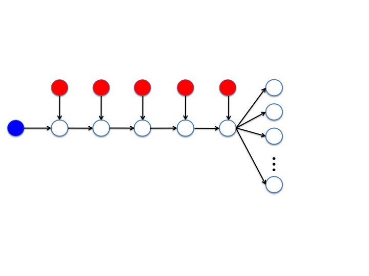
Figure 5: Illustration of the construction in the proof of Theorem 6. Left: Basic gadget. Right: Equilibrium construction.

We have thus shown that even when the switching function is “nice” (linear), even slight punishment in the selection function can lead to unbounded Budget Multiplier. Recall that we require switching and selection functions to be 0 (1, respectively) on input 0 (respectively) and increasing, and additionally that $g(1/2)=1$. The following theorem shows that if $f$ is allowed to be a sufficiently convex function, then the Budget Multiplier is again unbounded for any selection function. This establishes the importance of concavity of $f$ for both the PoA and Budget Multiplier.

Theorem 6

Let the switching $f$ satisfy $f(1/2)=0$ and $f(1)=1$. Then for any value $V>0$, there exists $G$ such that the Budget Multiplier is greater than $V$.

Let the Blue player have 1 initial infection and the Red player have $K\geq 2$ (the proof can be generalized to any unequal initial budgets, which we comment on below). Consider the directed graph shown in the left panel of Figure 5, where we have arranged the 1 Blue and $K$ Red seeded nodes in a particular configuration. Aside from the initially infected vertices, this graph consists of a directed chain of $K$ vertices, whose final vertex then connects to a large number $N\gg K$ of terminal vertices. Let us update each vertex in the chain from left to right, followed by the terminal vertices.

Let us first compute the expected payoffs for the two players in this configuration. First, note that since $f(1)=1$, it is certain that every vertex in the chain will be infected in sequence, followed by all of the terminal vertices; the only question is which player will win the most. By choosing $N\gg K$ we can ignore the infections in the chain and just focus on the terminal vertices, which will be won by whichever player infects the final chain vertex. It is easy to see that the probability this vertex is won by Blue is $1/2^{K}$, since Blue must “beat” a competing Red infection at every vertex in the chain. Thus the expected payoffs are approximately $N/2^{K}$ for Blue and $N(1-1/2^{K})$ for Red. If this configuration were an equilibrium, the Budget Multiplier would thus be $2^{K}/K$, which can be made as large as desired by choosing $K$ large enough.

However, this configuration is not an equilibrium — clearly, either player would be better off by simplifying initially infecting the final vertex of the chain, thus winning all the terminal vertices. This is fixed by the construction shown in the right panel of Figure 5, where we have replicated the chain and terminal vertices $M$ times, but have only the original $K+1$ seeded nodes as common “inputs” to all of these replications. Notice that now if either player defects to an uninfected vertex, neither player will receive any infections in any of the other replications, since now there is a missing “input infection” and reaching the terminal vertices requires all $K+1$ input infections since $f(1/2)=0$ (each chain vertex has two inputs, and if either is uninfected, the chain of infections halts). Similarly, if either player attempts to defect by invading the seeded nodes of the other player, there will be no payoff for either player in any of the replications. Thus the most Blue can obtain by deviation is $N$ (moving its one infection to the final chain vertex of a single replication), while the most Red can obtain is $KN$ (moving all of their infections to the final chain vertices of $K$ replications. The equilibrium requirements are thus $M(N/2^{K})>N$ for Blue, and $MN(1-1/2^{k})>KN$ for Red. The Blue requirement is the stronger one, and yields $M>2^{K}$. The Budget Multiplier for this configuration is the same as for the single replication case, and thus if we let $K$ be as large as desired and choose $M>2^{K}$, we can make the Budget Multiplier exceed any value.  (Theorem 6)

It is worth noting that even if the Blue player has $L>1$ seeded nodes, and we repeat the construction above with chain length $K+L-1$, but with Blue forced to play at the beginning of the chain, followed by all the Red infections, the argument and calculations above are unchanged: effectively, Blues $L$ seeded nodes are no better than 1 infection, because they are simply causing a chain of $L-1$ Blue infections before then facing the chain of $K$ Red inputs. In fact, even if we let $L\gg K$, Blue’s payoff will still be a factor of $1/2^{K}$ smaller than Red’s. Thus in some sense the theorem shows that if $f$ is sufficiently convex, not only is the Budget Multiplier unbounded, but the much smaller initial budget may yield arbitrarily higher payoffs!

7 Concluding Remarks

We have developed a general framework for the study of competition between firms who use their resources to maximize adoption of their product by consumers located in a social network. This framework yields a very rich class of competitive strategies, which depend in subtle ways on the dynamics, the relative budgets of the players and the structure of the social network. We identified properties of the dynamics of local adoption under which resource use by players is efficient or unboundedly inefficient. Similarly, we identified adoption dynamics for which networks neutralize or dramatically accentuate ex-ante resource difference across players.

There are a number of other questions which can be fruitfully investigated within our framework. One obvious direction is to understand the structure of equilibria in greater detail, and in particular how it is related to network structure. While our results on the PoA and Budget Multiplier demonstrate that network structure can interact in dramatic ways with the switching and selection functions at equilibrium, a more general and detailed understanding would be of interest.

Our model assumed that players’ budgets are exogenously given. In many contexts, the budget may itself be a decision variable. It is important to understand if endogenous budgets would aggravate or mitigate the problem of high PoA. Large network advantages from resources (reflected in high Budget Multiplier) create an incentive to increase budgets, and may be self-neutralizing.

Other interesting directions include algorithmic issues such as computing equilibria and best responses in our framework, and how their difficulty depends on the switching and selection functions; and the multi-stage version of our game, in which the two firms may gradually spend their seed budgets in a way that depends on the evolving state of the network.

One criticism of the model presented here is that while we assume rationality on the part of the competing firms, consumers (represented by the vertices in the social network) behave in a purely stochastic, non-rational fashion. In this appendix, we sketch natural cases in which these stochastic decisions can actually be provided with rational microeconomic models. We illustrate how the switching and selection functions $f$-$g$ may be founded upon optimal decisions made by consumers located in social networks. Information sharing about products and direct advantages accruing from adopting compatible products are two important ingredients of local social influence.

Example 1: Information Sharing: Consumers are looking for a good whose utility depends on its quality; the quality is known or easily verified upon inspection (such products are referred to as ‘search’ goods), but its availability may not be known. Examples of such products might be televisions and desktop computers. Consumers search on their own and they also get information from their friends and neighbors. Suppose for simplicity that the consumer talks to one friend before making his decision. As he runs into friends at random, other things being equal, the probability of adopting a product is equal to the probability of meeting someone who has adopted it. This probability is in turn given by the fraction of neighbors who have adopted the product. This corresponds to the case where $f$ and $g$ are both linear.

Example 2: Information Sharing and Payoff Externalities. Consumers are choosing between goods whose utility depends on how many other consumers have adopted the same product. Prominent examples include social networking sites. Suppose products offer stand alone advantage $v$, and a adoption related reward which is equal to the number of Reds or the number of Blues. Consumer picks neighbors at random. If neighbor is Red or Blue, then consumer becomes aware of product market. There is a small cost (relative to $v$) at which he can ask all his neighbors about their status. He then compares the adoption rates of the two products and given the benefits to being in a larger (local) network, the consumer selects the more popular product. This situation gives rise to an $f$ which is increasing and concave in the fraction of adopters, while $g$ is polarizing (close to a winner-take-it all).

We leave to future work the formulation of further and richer microeconomic consumer models, including a fully game-theoretic formulation over both firms and consumers.

References

- [1] Ballester, C., A. Calvo-Armengol, and Y. Zenou (2006), Who’s Who in Networks. Wanted: The Key Player, Econometrica, 74, 5, 1403-1417.
- [2] Bharathi, S., D. Kempe and M. Salek (2007), Competitive Influence Maximization in Social Networks, Internet and Network Economics Lecture Notes in Computer Science, 4858, 306-311.
- [3] Borodin, A., Filmus, Y., Oren, J. (2010) Threshold Models for Competitive Influence in Social Networks, Proc. Workshop on Internet and Network Economics (WINE)
- [4] Butters, G. (1977), Equilibrium Distribution of Prices and Advertising, Review of Economic Studies, 44, 465-492.
- [5] Chasparis, G. and Shamma, J. (2010), Control of Preferences in Social Networks", 49th IEEE Conference on Decision and Control.
- [6] Coleman, J. (1966), Medical Innovation: A Diffusion Study. Second Edition, Bobbs-Merrill. New York.
- [7] Conley, T. and C. Udry (2010), Learning about a New Technology: Pineapple in Ghana. American Economic Review, .
- [8] Carnes, T., Nagarajan, C., Wild, S., van Zuylen, A. (2007), Maximizing Influence in a Competitive Social Network: A Follower’s Perspective. Proc. Ninth ACM Conference on Electronic Commerce (EC), pages 351-360.
- [9] Dubey, P., Garg, R., De Meyer, B. (2006), Competing for Customers in a Social Network: The Quasi-linear Case. Proc. Workshop on Internet and Network Economics (WINE)
- [10] Dubey, P. (1986), Inefficiency of Nash Equilibria. Mathematics of Operations Research., 11, 1, 1 8.
- [11] Feick, L.F. and L.L. Price (1987), The Market Maven: A Diffuser of Marketplace Information. Journal of Marketing, 51(1), 83-97.
- [12] Foster, A.D. and M.R. Rosenzweig (1995), Learning by Doing and Learning from Others: Human Capital and Technical Change in Agriculture. Journal of Political Economy, 103(6), 1176-1209.
- [13] Galeotti, A., and S. Goyal (2009), Influencing the Influencers: a Theory of Strategic Diffusion, Rand Journal of Economics, 40, 3,
- [14] Godes D. and D. Mayzlin (2004), Using Online Conversations to Study Word of Mouth Communication. Marketing Science, 23(4), 545-560.
- [15] Granovetter, M. (1978), Threshold Models of Collective Behavior, American Journal of Sociology, 83, 6, 1420-1443.
- [16] Grossman, G. and C. Shapiro (1984), Informative Advertising with Differentiated Products. Review of Economic Studies, 51, 63-82.
- [17] Heidari, H. (2012), A Note on the Competitive Contagion Problem. Personal communication.
- [18] Koutsoupias, E., and C. H. Papadimitriou (1999), Worst-case Equilibria, STACS.
- [19] Kempe, D., J. Kleinberg, E. Tardos. (2003), Maximizing the Spread of Influence through a Social Network. Proc. 9th ACM SIGKDD Intl. Conf. on Knowledge Discovery and Data Mining.
- [20] Kempe, D., J. Kleinberg, E. Tardos (2005), Influential Nodes in a Diffusion Model for Social Networks. Proc. 32nd International Colloquium on Automata, Languages and Programming (ICALP).
- [21] Mossel, E., Roch, S. (2007), Submodularity of Influence in Social Networks: From Local to Global. SIAM J. Computing, 39(6):2176-2188.
- [22] Reingen, P.H., B.L. Foster, J.J. Brown and S.B. Seidman (1984), Brand Congruence in Interpersonal Relations: A Social Network Analysis. The Journal of Consumer Research, 11(3), 771-783.
- [23] Roughgarden, T., Tardos, E. (2000), How Bad is Selfish Routing? Proc. 41st Annual IEEE Symposium on Foundations of Computer Science (FOCS).
- [24] Skaperdas, S. (1996), Contest Success Functions, Economic Theory, 7, 2, 283-290.
- [25] Tullock, G. (1967), The Welfare Costs of Tariffs, Monopolies, and Theft, Western Economic Journal 5, 3, 224-232.
- [26] Tullock, G. (1980), Efficient Rent Seeking, Towards a theory of the rent-seeking society, edited by Buchanan, J., Tollison, R., and Tullock, G., Texas A&M University Press.
- [27] Vetta, A. (2002), Nash Equilibria in Competitive Societies with Applications to Facility Location, Traffic Routing and Auctions. Proceedings of the 43rd Symposium on the Foundations of Computer Science (FOCS), 416-425.