Multifractals Competing with Solitons on Fibonacci Optical Lattice

Abstract

We study the stationary states for the nonlinear Schrödinger equation on the Fibonacci lattice which is expected to be realized by Bose-Einstein condensates loaded into an optical lattice. When the model does not have a nonlinear term, the wavefunctions and the spectrum are known to show fractal structures. Such wavefunctions are called critical. We present a phase diagram of the energy spectrum for varying the nonlinearity. It consists of three portions, a forbidden region, the spectrum of critical states, and the spectrum of stationary solitons. We show that the energy spectrum of critical states remains intact irrespective of the nonlinearity in the sea of a large number of stationary solitons.

1 Introduction

The realization of Bose-Einstein condensation (BEC) in optical lattices has opened a new avenue for studying a variety of phenomena in condensed matter systems [1, 2]. A major advantage of using ultracold atomic gases is that one can control the interatomic interactions and the lattice parameters in an extremely clean environment. This high degree of tunability enables one to study BEC in artificially designed structures which cannot be achieved in conventional solids. For instance, the one-dimensional bichromatic potential has been realized in a system of ⁸⁷Rb atoms [3], and such a quasiperiodic potential has been studied theoretically [4] in the context of BEC. More recently, a new method for creating potentials through a holographic mask was introduced [5]. Using this technique, it seems feasible to experimentally generate exotic structures such as the Fibonacci lattice [6, 7, 8] and the Penrose tiling [9, 10] which are of interest as one- and two-dimensional quasicrystals, respectively.

These low-dimensional quasicrystals have attracted considerable theoretical attention since there appear fractal wavefunctions which are neither extended nor localized [8, 11]. They are called critical states. The rapid progress in the study of BEC can set a stage for exploring these exotic states in experiments. The new ingredient that appears in the system of BEC is the nonlinearity caused by interatomic interactions which can be tuned by the Feshbach resonance. One might expect that fractal wavefunctions are fragile and are easily destroyed by the nonlinearity. Surprisingly, this is not the case. In fact, we demonstrate that there indeed exist critical states on the Fibonacci optical lattice. This is intended to stimulate experimental efforts to observe critical states in a cold-atom setup.

In order to describe a Bose-Einstein condensate on the Fibonacci optical lattice, we resort to the nonlinear Schrödinger equation with on-site potentials arranged in the Fibonacci sequence [13]. In the absence of the nonlinear term, it is known that all the eigenstates are critical, and that the spectrum shows a fractal structure [8, 11]. More precisely, the spectrum is singular continuous [11, 14] and called the Cantor spectrum. In order to elucidate the effect of nonlinearity on the critical states, we numerically solve the stationary nonlinear Schrödinger equation. As mentioned above, our numerical results show that the critical states persist despite the presence of the nonlinearity in the sea of stationary solitons [15, 13]. With the aid of mathematical tools, we show that for any critical state, the “eigenenergy” must be included in the Cantor spectrum of the Schrödinger equation without nonlinearity. Further, we determine a forbidden region for the eigenenergy and the strength of the nonlinearity. Putting these together, we present a phase diagram of the energy spectrum for varying the nonlinearity. (See Fig. 4 in Sec. 6.) The energy spectrum of the critical states retains its profile irrespective of the nonlinearity, while the number of the stationary solitons increases enormously as the nonlinearity increases. One might think that the presence of the sea of solitons makes it difficult to experimentally detect the fractal profiles of the critical states. However, in the neighborhood of the forbidden region, such an experimental detection is expected to be possible. (See Sec. 6 and Fig. 4 for details.)

Throughout the present paper, we will not treat dynamical properties of the wavefunctions for the nonlinear Schrödinger equation. However, we think we should at least stress that knowledge of the stationary states is not sufficient for understanding the dynamics such as diffusion of wave packets in quasiperiodic or random environment [16, 17, 18, 19, 20, 21]. For the random nonlinear Schrödinger equation, see a recent review [22].

The present paper is organized as follows: The precise definition of the nonlinear Schrödinger equation which we consider in the present paper is given in Sec. 2. In Sec. 3, the numerical solutions of the model are obtained. In Sec. 4, we apply the multifractal analysis to the solutions so obtained. The mathematical analysis for the model is given in Sec. 5. Our results are summarized as the phase diagram in Sec. 6. Section 7 is devoted to summary and conclusion. In A, we discuss effects of nonlinearity on localization.

2 Preliminary

Let us consider the one-dimensional chain which is determined by the Fibonacci rule. The $\ell$-th chain, $S_{\ell}$, $\ell\!=\!1,2,\ldots$, consists of two symbols, $A$ and $B$, and is constructed by the recursion, $S_{\ell\!+\!1}\!=\!S_{\ell}S_{\ell\!-\!1}$, with the initial condition, $S_{0}\!=\!B$ and $S_{1}\!=\!A$:

$$S_{1}\!=\!A,~{}~{}S_{2}\!=\!AB,~{}~{}S_{3}\!=\!ABA,~{}~{}S_{4}\!=\!ABAAB,~{}\ldots$$

We denote by $N\!=\!N_{\ell}$ the number of symbols in $S_{\ell}$. Clearly, $N_{\ell}$ is equal to the Fibonacci number because they satisfy $N_{\ell\!+\!1}\!=\!N_{\ell}\!+\!N_{\ell\!-\!1}$ with $N_{0}\!=\!N_{1}\!=\!1$. In the limit $\ell\!\rightarrow\!\infty$, the Fibonacci chain is neither random nor periodic. In fact, it is quasiperiodic.

The nonlinear Schrödinger equation for stationary states, $(\psi_{1},\psi_{2},\ldots,\psi_{N})$, on the Fibonacci chain is given by

$$t(\psi_{i+1}+\psi_{i-1})+V_{i}\psi_{i}+g|\psi_{i}|^{2}\psi_{i}=E\psi_{i}\quad\mbox{for}\ \ i=1,2,\ldots,N,$$ (1)

where the hopping integral $t$ and the coupling constant $g$ are real, $E$ is an “eigenenergy” [23, 24, 25], and the on-site potential $V_{i}$ is given by

$$V_{i}=\begin{cases}V_{A}&\text{if $i$-th symbol of $S_{\ell}$ is $A$,}\\ V_{B}&\text{if $i$-th symbol of $S_{\ell}$ is $B$}\end{cases}$$

with real $V_{A}$ and $V_{B}$. We impose the Dirichlet boundary conditions, $\psi_{0}\!=\!\psi_{N\!+\!1}\!=\!0$, or the periodic boundary condition, $\psi_{N\!+\!i}\!=\!\psi_{i}$. We choose the normalization of the wavefunctions as $\sum_{i=1}^{N}|\psi_{i}|^{2}\!=\!1$.

3 Numerical analysis

Using the shooting method, we numerically solve (1) with the Dirichlet boundary condition. We choose $V_{A}\!=\!-\!1$, $V_{B}\!=\!+\!1$ and $t\!=\!1$. For fixed $E$ and $g$, we continuously vary the amplitude $\psi_{1}$ so as to hit $\psi_{N\!+\!1}\!=\!0$ at site $N\!+\!1$. A solution so obtained does not satisfy $\sum_{i=1}^{N}|\psi_{i}|^{2}\!=\!1$ in general. So we set $\psi_{i}\!=\!\lambda\psi_{i}^{\prime}$ with $\lambda>0$ so as to satisfy $\sum_{i=1}^{N}|\psi_{i}^{\prime}|^{2}\!=\!1$. Then the coupling constant is given by $g^{\prime}\!=\!\lambda^{2}g$. In the following we drop primes.

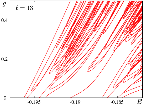
Figure 1: Numerical solutions of (1) are plotted in the $E$-$g$ plane near the band center for chain length $N_{\ell}\!=\!377$ with $\ell\!=\!13$.

The numerical results for eigenenergies $E$ are plotted in the $E$-$g$ plane in Fig. 1. Each eigenenergy $E$ is an increasing function of $g$. This is a consequence of the positivity of the nonlinear term. Unlike the linear Schrödinger equation, there appear many solutions whose number is beyond the total number of the sites of the chain $N$. These contain a large number of localized states. Since the localized states are due to the nonlinearity, we call them solitons. This phenomenon is already known as the appearance of localized states for lattice systems [15, 13]. There are solutions with different spatial profiles as shown in Figs. 2. It seems likely that all the states, extended, critical, soliton, and surface states, mix like a complicated “soup”. However, we will show below that extended states are absent, whereas critical states and solitons exist. The surface states exist only for a system with the Dirichlet boundary condition.

For the Harper model [26, 27] at criticality, effects of nonlinearity were discussed in [28]. Their numerical results show that the eigenmodes can be classified into two families: the conventional modes which are continuously connected to those in the corresponding linear model and new modes that have no origin in the linear model. If the latter modes are interpreted as stationary solitons due to the nonlinearity as in our case, their results of [28] are consistent with ours.

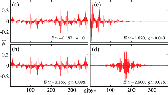
Figure 2: The left column shows critical wavefunctions in (a) a linear case and (b) a nonlinear case. The right column shows localized wavefunctions of (c) a surface state and (d) a soliton in a nonlinear case. All the data are for chain length $N_{\ell}\!=\!377$ with $\ell\!=\!13$.

4 Multifractal analysis

As is well known, the scaling analysis which is called multifractal analysis [29, 30] is a very useful tool to determine whether or not a given wavefunction is critical [31]. Relying on this analysis, we numerically check the existence of critical states. We expect that the wavefunction which is shown in Fig. 2 (b) with $g\!\neq\!0$ leads to a critical state in the infinite-length limit of the chain. In the multifractal analysis, a wavefunction is characterized by $f(\alpha)$. For a wavefunction $\bm{\psi}\!=\!(\psi_{1},\ldots,\psi_{N})$, the number of sites $i$ satisfying $|\psi_{i}|^{2}\!\sim\!N^{-\alpha}$ is assumed to be proportional to $N^{f_{\ell}(\alpha)}$. The subscript $\ell$ and the chain length $N$ are related through $N\!=\!N_{\ell}$ with the Fibonacci number $N_{\ell}$ whose definition is given in Sec. 2. We denote by $f(\alpha)$ the infinite-length limit of $f_{\ell}(\alpha)$. Using $f(\alpha)$, one can determine the character of a given wavefunction as follows:

• An extended state shows a single point, $(f,\alpha)\!=\!(1,1)$.

• A localized state shows two points, $(f,\alpha)\!=\!(0,0)$ and $(1,\infty)$.

• A critical state shows a sequence of smooth curves $f_{\ell}(\alpha)$ which do not fall into the above two categories in the infinite-length limit.

As to critical states, the corresponding sequence does not necessarily converge to some $f(\alpha)$. But, it is known that $f_{\ell}(\alpha)$ for a wavefunction with a multifractal character converges to a single smooth curve $f(\alpha)$. Our numerical results of $f_{\ell}(\alpha)$ are shown in Fig. 3. The results show that the wavefunctions are critical because the behavior of the sequence of $f_{\ell}(\alpha)$ is totally different from those of $f_{\ell}(\alpha)$ for extended and localized states [31]. In consequence, the critical states persist in spite of the nonlinear term.

However, it is still unclear whether or not the state shows perfect multifractality [32] within our numerical analysis since the right side of the profile of $f_{\ell}(\alpha)$ is oscillating as $\ell$ increases, and does not seem to converge to a single smooth curve in the limit $\ell\rightarrow\infty$. The oscillation in Fig. 3 can be explained as the effect of the Dirichlet boundary condition as follows: We treat only the case of the linear Schrödinger equation, i.e., (1) with $g=0$. We impose the periodic boundary condition. Let ${\bm{\psi}}\!=\!(\psi_{1},\ldots,\psi_{N})$ and ${\bm{\psi}}^{\prime}\!=\!(\psi_{1}^{\prime},\ldots,\psi_{N}^{\prime})$ be two independent eigenvectors with the eigenvalues, $E$ and $E^{\prime}$, respectively. We assume that $E$ is nearly equal to $E^{\prime}$, and that $|\psi_{1}|^{2}\sim N^{-\alpha_{1}}$ and $|\psi_{1}^{\prime}|^{2}\sim N^{-\alpha_{1}^{\prime}}$ with $\alpha_{1}>\alpha_{1}^{\prime}>0$. Consider

$${\bm{\varphi}}=\bm{\psi}-\frac{\psi_{1}}{\psi_{1}^{\prime}}{\bm{\psi}}^{\prime}.$$ (2)

Then, ${\bm{\varphi}}$ satisfies the Dirichlet boundary condition, $\varphi_{1}=\varphi_{N+1}=0$. We assume that both of ${\bm{\psi}}$ and ${\bm{\psi}}^{\prime}$ show the same $f_{\ell}(\alpha)$. In order to distinguish $f_{\ell}(\alpha)$ of the wavefunction ${\bm{\varphi}}$ from that of $\bm{\psi}$ or ${\bm{\psi}}^{\prime}$, we write ${\tilde{f}}_{\ell}(\alpha)$ for $f_{\ell}(\alpha)$ of ${\bm{\varphi}}$.

We want to show that ${\tilde{f}}_{\ell}(\alpha)$ is not necessarily equal to $f_{\ell}(\alpha)$, and the deviation strongly depends on $\alpha_{1}$ and $\alpha_{1}^{\prime}$. Consider the probability density $|\varphi_{i}|^{2}$ at the site $i$. The contribution of the first term $\bm{\psi}$ in the right-hand side of (2) is written

$$|\psi_{i}|^{2}\sim N^{-\alpha_{i}}$$ (3)

with some $\alpha_{i}>0$. The contribution of the second term is written

$$\left|\frac{\psi_{1}}{\psi_{1}^{\prime}}\psi_{i}^{\prime}\right|^{2}\sim N^{-(\alpha_{1}-\alpha^{\prime}_{1})}N^{-\alpha^{\prime}_{i}}=N^{-(\alpha_{i}^{\prime}+\Delta\alpha)}$$ (4)

with $\Delta\alpha:=\alpha_{1}-\alpha_{1}^{\prime}$, where we have assumed

$$\left|\psi_{i}^{\prime}\right|^{2}\sim N^{-\alpha_{i}^{\prime}}$$ (5)

with some $\alpha_{i}^{\prime}>0$. Therefore, we naively expect that the number of the site $i$ satisfying $|\varphi_{i}|^{2}\sim N^{-\alpha}$ is given by

$$N^{{\tilde{f}}_{\ell}(\alpha)}\sim\begin{cases}N^{f_{\ell}(\alpha)}&\mbox{if}\ \ f_{\ell}(\alpha)\geq f_{\ell}(\alpha-\Delta\alpha),\\ N^{f_{\ell}(\alpha-\Delta\alpha)}&\mbox{if}\ \ f_{\ell}(\alpha)<f_{\ell}(\alpha-\Delta\alpha).\end{cases}$$ (6)

However, the behavior in the second case is questionable. Clearly, from (4), the second case occurs for large $\alpha$. Further, if $\alpha=\alpha_{i}^{\prime}+\Delta\alpha>\alpha_{i}$, then one has $|\varphi_{i}|^{2}\sim N^{-\alpha_{i}}$. In such a case, the second term in the right-hand side of (2) does not contribute to ${\tilde{f}}_{\ell}(\alpha)$ although $\alpha_{i}^{\prime}+\Delta\alpha=\alpha$. From these observations, we conclude that $N^{f_{\ell}(\alpha-\Delta\alpha)}$ in the second case of (6) is reduced to some value $N^{{\tilde{f}}_{\ell}(\alpha)}$ which satisfies

$$N^{f_{\ell}(\alpha)}\leq N^{{\tilde{f}}_{\ell}(\alpha)}\leq N^{f_{\ell}(\alpha-\Delta\alpha)}.$$ (7)

In fact, as is well known, ${\tilde{f}}_{\ell}(\alpha)$ must become a smooth curve having a single peak. To summarize, we obtain

$$\begin{cases}{\tilde{f}}_{\ell}(\alpha)=f_{\ell}(\alpha)&\mbox{if}\ \ f_{\ell}(\alpha)\geq f_{\ell}(\alpha-\Delta\alpha),\\ f_{\ell}(\alpha)\leq{\tilde{f}}_{\ell}(\alpha)\leq f_{\ell}(\alpha-\Delta\alpha)&\mbox{if}\ \ f_{\ell}(\alpha)<f_{\ell}(\alpha-\Delta\alpha).\end{cases}$$ (8)

This explains the oscillation of $f_{\ell}(\alpha)$ on the right side of the profile in Fig. 3. Thus the oscillation of the profile of the right side is due to the Dirichlet boundary condition.

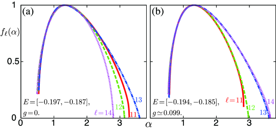
Figure 3: (color online) $f_{\ell}(\alpha)$ in (a) linear cases and (b) nonlinear cases. These numerical results show that the corresponding states are critical. Even in the linear case, $f_{\ell}(\alpha)$ oscillates as $\ell$ increases.

5 Mathematical analysis

We want to elucidate the spectral structure of Fig. 1, and extrapolate it to the infinite-length limit of the chain (Fig. 4).

First of all, it is practical to review the known results in the linear case, $g\!=\!0$. Consider first the linear Schrödinger equation with the periodic boundary condition. In the infinite-length limit, all of the stationary states are critical and the energy spectrum becomes a singular continuous Cantor set. On the other hand, as to the Dirichlet boundary condition, the surface states appear and their eigenenergies form a pure point spectrum in addition to the Cantor spectrum of the critical states.

In this section, we prove three theorems for the nonlinear Schrödinger equation: Theorem 1 states that there exists a forbidden region for two parameters, energy and nonlinearity, such that the nonlinear Schrödinger equation (1) with the periodic boundary condition has no solution. In the infinite-length limit, this forbidden region for the spectrum is common to both of the periodic and Dirichlet boundary conditions except for the spectrum of the surface states as we will show in Theorem 3. Theorem 2 states that an eigenenergy of a critical or extended state for the nonlinear Schrödinger equation is included in the spectrum in the case of $g\!=\!0$ in the infinite-length limit. This leads to the robustness of the critical states irrespective of the nonlinearity.

Consider the linear Schrödinger equation,

$$t(\psi_{i+1}+\psi_{i-1})+V_{i}\psi_{i}=E\psi_{i},$$ (9)

i.e., (1) with $g\!=\!0$ and with the periodic boundary condition. We denote the Hamiltonian for (9) by $H_{0}$. We also denote the $N$ eigenvalues by $\mathcal{E}_{m}$, $m\!=\!1,2,\ldots,N$, satisfying $\mathcal{E}_{j}\!\leq\!\mathcal{E}_{k}$ for $j\!<\!k$. Define a set of real numbers,

$$\Gamma :=(-\infty,\mathcal{E}_{1})\cup(\mathcal{E}_{1}+g,\mathcal{E}_{2})\cup\cdots\cup(\mathcal{E}_{N-1}+g,\mathcal{E}_{N})\cup(\mathcal{E}_{N}+g,+\infty),$$ (10)

for $g\!\geq\!0$, where $(\cdot,\cdot)$ denotes an open interval. Here, if $g\geq\mathcal{E}_{n\!+\!1}-\mathcal{E}_{n}$, then $(\mathcal{E}_{n}\!+\!g,\mathcal{E}_{n\!+\!1})=\emptyset$ for $n\!=\!1,2,\ldots,N\!-\!1$.

Theorem 1.

Let $g>0$. Let $E$ be an eigenenergy of the nonlinear Schrödinger equation (1) with the periodic boundary condition. Then, $E\!\notin\!\Gamma$.

Proof.

Let $(\tilde{\psi}_{1},\ldots,\tilde{\psi}_{N})$ be a solution of the nonlinear Schrödinger equation (1) with the eigenenergy $\tilde{E}$. As in the assumption, we impose the periodic boundary condition. Then one can find $n\in\!\{1,2,\ldots,N\}$ which satisfies $\mathcal{E}_{n}\!\leq\!\tilde{E}\!<\!\mathcal{E}_{n\!+\!1}$, where $\mathcal{E}_{N\!+\!1}\!:=\!+\!\infty$. Therefore, it is sufficient to show that $\tilde{E}\!\leq\!\mathcal{E}_{n}\!+\!g$. Write $U_{i}\!=\!|\tilde{\psi}_{i}|^{2}$, and consider the linear Schrödinger equation,

$$t(\psi_{i+1}+\psi_{i-1})+V_{i}\psi_{i}+gU_{i}\psi_{i}=E\psi_{i},$$ (11)

with the additional potential $gU_{i}$, and with the periodic boundary condition. Namely, we fix the additional potential $gU_{i}$ by using the solution $(\tilde{\psi}_{1},\ldots,\tilde{\psi}_{N})$ of the nonlinear Schrödinger equation. Clearly, $(\tilde{\psi}_{1},\ldots,\tilde{\psi}_{N})$ is a particular solution of the equation (11) with the eigenvalue $\tilde{E}$. We denote by $\tilde{H}$ the Hamiltonian for (11), and denote the $N$ eigenvalues by $\tilde{\mathcal{E}}_{m}$, $m\!=\!1,2,\ldots,N$, satisfying $\tilde{\mathcal{E}}_{j}\!\leq\!\tilde{\mathcal{E}}_{k}$ for $j\!<\!k$.

Note that the Hamiltonian $\tilde{H}$ is written as $\tilde{H}\!=\!H_{0}\!+\!gU$ with $U\!=\!\textrm{diag}(U_{1},\!U_{2},\!\ldots,\!U_{N})$. By the positivity of $gU$, we have $H_{0}\!\leq\!\tilde{H}$. As is well known, by applying the min-max principle to this type of an operator inequality, one can get an inequality between their eigenvalues. In the present case, we obtain $\mathcal{E}_{n\!+\!1}\!\leq\!\tilde{\mathcal{E}}_{n\!+\!1}$. Combining this, the assumption $\tilde{E}\!<\!\mathcal{E}_{n\!+\!1}$ and the fact that $\tilde{E}$ is the eigenvalue of $\tilde{H}$, we obtain $\tilde{E}\!\leq\!\tilde{\mathcal{E}}_{n}$.

On the other hand, we have the bound, $\tilde{H}\!\leq\!H_{0}\!+\!g$. Applying the min-max principle again, we obtain $\tilde{\mathcal{E}}_{n}\!\leq\!\mathcal{E}_{n}\!+\!g$. Combining this with the above result $\tilde{E}\!\leq\!\tilde{\mathcal{E}}_{n}$, we obtain the desired bound $\tilde{E}\!\leq\!\mathcal{E}_{n}\!+\!g$. ∎

Thus the nonlinear Schrödinger equation (1) has no solution in the region

$$\tilde{\Gamma}\!:=\!\{(E,g)|\ E\!\in\!\Gamma,g\!\geq\!0\}$$ (12)

for two parameters, energy and nonlinearity. The region $\tilde{\Gamma}$ is depicted as the non-colored region in Fig. 4. by replacing “periodic” to “Dirichlet” in the proof. The forbidden region of the energy spectrum for the Dirichlet boundary condition will be treated in Theorem 3 below. One might think that Theorem 1 is not too surprising because the deviation of the eigenenergy is less than or equal to $g$ from $U_{i}\!=\!|\psi_{i}|^{2}\!\leq\!1$. We stress that the statement of Theorem 1 includes that all the eigenenergies of the stationary solitons which are caused by the nonlinearity are also forbidden in the region $\tilde{\Gamma}$. The key idea of the proof is to introduce the potential $gU$ into the linear Schrödinger equation. This enables us to apply the min-max principle to nonlinear problems for the first time.

In order to determine whether a given state is critical or not, we must treat the infinite-length limit. Let $\{N(k)\}_{k\!=\!1}^{\infty}$ be an increasing sequence of the length $N\!=\!N(k)$ of the present chain. Let $\tilde{\bm{\psi}}^{(k)}\!=\!(\tilde{\psi}_{1}^{(k)},\tilde{\psi}_{2}^{(k)},\ldots,\tilde{\psi}_{N(k)}^{(k)})$ be a solution of the nonlinear Schrödinger equation (1) with the eigenenergy $\tilde{E}^{(k)}$ for the chain with the length $N(k)$. Write $U_{i}^{(k)}\!=\!|\tilde{\psi}_{i}^{(k)}|^{2}$, and $U_{\mathrm{max}}^{(k)}\!=\!\max_{i}U_{i}^{(k)}$. We assume that $\lim_{k\!\rightarrow\!\infty}U_{\mathrm{max}}^{(k)}$ exists. If not so, we take a subsequence. We say that the wavefunction $\tilde{\bm{\psi}}^{(k)}$ is localized if $\lim_{k\!\rightarrow\!\infty}U_{\mathrm{max}}^{(k)}\!>\!0$, and $\tilde{\bm{\psi}}^{(k)}$ is critical or extended if $\lim_{k\!\rightarrow\!\infty}U_{\mathrm{max}}^{(k)}\!=\!0$. We write $H_{0,N(k)}^{P}$ for $H_{0}$ of (9) with the length $N(k)$ and with the periodic boundary condition. The spectrum of $H_{0,N(k)}^{P}$ is given by $\sigma(H_{0,N(k)}^{P})\!:=\!\{\mathcal{E}_{1},\ldots,\mathcal{E}_{N(k)}\}$.

Theorem 2.

Consider the nonlinear Schrödinger equation (1) with periodic/Dirichlet boundary condition. If a sequence $\{\tilde{\bm{\psi}}^{(k)}\}_{k\!=\!1}^{\infty}$ of the solutions is critical or extended in the infinite-length limit of the chain, $k\!\rightarrow\!\infty$, then the distance between the eigenenergy $\tilde{E}^{(k)}$ of $\tilde{\bm{\psi}}^{(k)}$ and the spectrum $\sigma(H_{0,N(k)}^{P})$ must go to zero in the limit $k\!\rightarrow\!\infty$.

Proof.

First consider the Hamiltonian $\tilde{H}_{N(k)}^{D}$ for the linear Schrödinger equation (11) with the Dirichlet boundary condition in the proof of Theorem 1 with the additional potential $U_{i}^{(k)}$ and with the length $N(k)$. Clearly, $\tilde{\bm{\psi}}^{(k)}$ is the eigenvector of $\tilde{H}_{N(k)}^{D}$ with the eigenvalue $\tilde{E}^{(k)}$. This yields

$$\left\langle\tilde{\bm{\psi}}^{(k)},\left(\tilde{H}_{N(k)}^{D}-H_{0,N(k)}^{P}\right)^{2}\tilde{\bm{\psi}}^{(k)}\right\rangle=\left\langle\tilde{\bm{\psi}}^{(k)},\left(\tilde{E}^{(k)}-H_{0,N(k)}^{P}\right)^{2}\tilde{\bm{\psi}}^{(k)}\right\rangle.$$ (13)

In order to obtain the lower bound for the right-hand side, we introduce the system of the complete orthonormal eigenvectors $\{\textbf{u}_{i}^{(k)}\}$ for $H_{0,N(k)}^{P}$. Namely,

$$H_{0,N(k)}^{P}\textbf{u}_{i}^{(k)}={\cal E}_{i}^{(k)}\textbf{u}_{i}^{(k)}$$ (14)

with the eigenvalues ${\cal E}_{i}~{}{(k)}$. Then, one has the expansion,

$$\tilde{\bm{\psi}}^{(k)}=\sum_{i}a_{i}^{(k)}\textbf{u}_{i}^{(k)}\quad\mbox{with}\ \ \sum_{i}\left|a_{i}^{(k)}\right|^{2}=1.$$ (15)

Using this, the right-hand side of (13) is evaluated as

$$\left\langle\tilde{\bm{\psi}}^{(k)},\left(\tilde{E}^{(k)}-H_{0,N(k)}^{P}\right)^{2}\tilde{\bm{\psi}}^{(k)}\right\rangle =\sum_{i}\left({\tilde{E}}^{(k)}-{\cal E}_{i}^{(k)}\right)^{2}\left|a_{i}^{(k)}\right|^{2}$$

$$\geq\min_{i}\left\{\left({\tilde{E}}^{(k)}-{\cal E}_{i}^{(k)}\right)^{2}\right\}.$$ (16)

Substituting this into the right-hand side of (13), we obtain

$$\left\langle\tilde{\bm{\psi}}^{(k)},\left(\tilde{H}_{N(k)}^{D}-H_{0,N(k)}^{P}\right)^{2}\tilde{\bm{\psi}}^{(k)}\right\rangle\geq\left[\mathrm{dist}(\sigma(H_{0,N(k)}^{P}),\tilde{E}^{(k)})\right]^{2}.$$ (17)

Next, let us obtain an upper bound for the left-hand side of (17). Note that $\tilde{H}_{N(k)}^{D}\!-\!H_{0,N(k)}^{P}\!=\!gU^{(k)}\!+\!\Delta H_{0,N(k)}$, where $\Delta H_{0,N(k)}\!=\!H_{0,N(k)}^{D}\!-\!H_{0,N(k)}^{P}$, i.e., the deference between the Hamiltonian $H_{0}$ (9) with the Dirichlet and with the periodic boundary conditions. Clearly, we have

$$\left\langle\tilde{\bm{\psi}}^{(k)},\left(\tilde{H}_{N(k)}^{D}-H_{0,N(k)}^{P}\right)^{2}\tilde{\bm{\psi}}^{(k)}\right\rangle =\left\langle\tilde{\bm{\psi}}^{(k)},g^{2}(U^{(k)})^{2}\tilde{\bm{\psi}}^{(k)}\right\rangle+\left\langle\tilde{\bm{\psi}}^{(k)},\Delta H_{0,N(k)}^{2}\tilde{\bm{\psi}}^{(k)}\right\rangle$$

$$+\left\langle\tilde{\bm{\psi}}^{(k)},\left(gU^{(k)}\Delta H_{0,N(k)}+\Delta H_{0,N(k)}gU^{(k)}\right)\tilde{\bm{\psi}}^{(k)}\right\rangle.$$ (18)

Since $gU^{(k)}$ and $\Delta H_{0,N(k)}$ are self-adjoint, Schwarz inequality yields

$$\left|\left\langle\tilde{\bm{\psi}}^{(k)},gU^{(k)}\Delta H_{0,N(k)}\tilde{\bm{\psi}}^{(k)}\right\rangle\right|^{2}\leq\left\langle\tilde{\bm{\psi}}^{(k)},g^{2}\left(U^{(k)}\right)^{2}\tilde{\bm{\psi}}^{(k)}\right\rangle\left\langle\tilde{\bm{\psi}}^{(k)},\Delta H_{0,N(k)}^{2}\tilde{\bm{\psi}}^{(k)}\right\rangle.$$ (19)

Substituting this into the right-hand side of (18), we have

$$\left\langle\tilde{\bm{\psi}}^{(k)},\left(\tilde{H}_{N(k)}^{D}-H_{0,N(k)}^{P}\right)^{2}\tilde{\bm{\psi}}^{(k)}\right\rangle$$

$$\leq\left\langle\tilde{\bm{\psi}}^{(k)},g^{2}(U^{(k)})^{2}\tilde{\bm{\psi}}^{(k)}\right\rangle+\left\langle\tilde{\bm{\psi}}^{(k)},\Delta H_{0,N(k)}^{2}\tilde{\bm{\psi}}^{(k)}\right\rangle$$

$$+2\sqrt{\left\langle\tilde{\bm{\psi}}^{(k)},g^{2}(U^{(k)})^{2}\tilde{\bm{\psi}}^{(k)}\right\rangle\left\langle\tilde{\bm{\psi}}^{(k)},\Delta H_{0,N(k)}^{2}\tilde{\bm{\psi}}^{(k)}\right\rangle}$$

$$=\left[\sqrt{\left\langle\tilde{\bm{\psi}}^{(k)},g^{2}(U^{(k)})^{2}\tilde{\bm{\psi}}^{(k)}\right\rangle}+\sqrt{\left\langle\tilde{\bm{\psi}}^{(k)},\Delta H_{0,N(k)}^{2}\tilde{\bm{\psi}}^{(k)}\right\rangle}\right]^{2}$$

$$\leq\left[|g|U_{\mathrm{max}}^{(k)}+|t|\sqrt{|\tilde{\psi}_{1}^{(k)}|^{2}+|\tilde{\psi}_{N(k)}^{(k)}|^{2}}\right]^{2}.$$ (20)

Combining this with the above bound (17), we obtain

$$\mathrm{dist}(\sigma(H_{0,N(k)}^{P}),\tilde{E}^{(k)})\leq|g|U_{\mathrm{max}}^{(k)}+|t|\sqrt{|\tilde{\psi}_{1}^{(k)}|^{2}+|\tilde{\psi}_{N(k)}^{(k)}|^{2}}.$$ (21)

If $\tilde{\bm{\psi}}^{(k)}$ is critical or extended, then this right-hand side is vanishing as $k\!\rightarrow\!\infty$.

Clearly, the same statement holds with the periodic boundary condition. In this case, the second term in the right-hand side of (21) does not appear since $\Delta H_{0,N(k)}\!=\!0$. ∎

We recall the well known fact that the spectrum $\sigma(H_{0,\infty}^{P})$ of the linear model in the infinite-length limit is singular continuous and has zero Lebesgue measure [6, 14, 11]. Theorem 2 states that all of the eigenenergies of critical or extended states in the nonlinear model fall into the set $\sigma(H_{0,\infty}^{P})$. This implies that the spectrum of critical or extended states in the nonlinear model in the infinite-length limit is a subset of $\sigma(H_{0,\infty}^{P})$, and has zero Lebesgue measure. In general linear models, a set of extended states is defined to have a spectrum having nonvanishing Lebesgue measure. Therefore, in this sense, there is no extended state in the present nonlinear model. However, we cannot conclude, from Theorem 2, that critical states indeed exist in the nonlinear model, and that all of the critical states in the linear model survive switching on the nonlinearity. This expectation is supported by our numerical results. Actually, as shown in Fig. 1, each of the critical states is continuously connected to that in the linear model for varying the strength of the nonlinearity. We also remark that eigenenergies of surface states due to the Dirichlet boundary condition can appear outside the spectrum $\sigma(H_{0,N(k)}^{P})$ in general.

The quantity $U_{i}=|\tilde{\psi}_{i}|^{2}$ which we introduced in the proof of Theorem 1 can be interpreted as an effective potential due to the nonlinearity. Since $U_{i}$ is vanishing for critical or extended states in the infinite-length limit, one might think that Theorem 2 is a trivial consequence of this fact. This is not true because the effect of the nonlinearity for the whole chain is estimated by $g\sum_{i}U_{i}$. Using the normalization condition $\sum_{i}|\tilde{\psi}_{i}|^{2}\!=\!1$, one has $g\sum_{i}U_{i}=g\sum_{i}|{\tilde{\psi}}_{i}|^{2}=g$. Thus, for a fixed $g$, the effect of the nonlinearity is ${\cal O}(1)$ irrespective of the length of the chain. We numerically check that the difference between critical wavefunctions $\bm{\psi}_{g\!=\!0}$ for $g\!=\!0$ and $\bm{\psi}_{g\!\neq\!0}$ for $g\!\neq\!0$ is ${\cal O}(1)$ in the sense of norm $||\bm{\psi}_{g\!\neq\!0}\!-\!\bm{\psi}_{g\!=\!0}||$ irrespective of the chain length. Here, $\bm{\psi}_{g\!\neq\!0}$ is continuously connected with $\bm{\psi}_{g\!=\!0}$. For a typical $\bm{\psi}_{g\!\neq\!0}$, we have $||\bm{\psi}_{g\!\neq\!0}\!-\!\bm{\psi}_{g\!=\!0}||\!\simeq\!0.208$ for $g\!\simeq\!0.098$ and $\ell\!=\!13$, where $\ell$ is defined in Sec. 2. Here the eigenenergy of $\bm{\psi}_{g\!=\!0}$ is $E\!\simeq\!-0.187$.

Roughly speaking, nonlinearity does not change the character of eigenstates of a linear Schrödinger equation. Since the property of the on-site potential is not used in the proof of Theorem 2, one can expect that nonlinearity does not change the localization character of eigenstates of a random linear Schrödinger equation, too. Actually, we can justify this type of statement for a certain class of nonlinear Schrödinger equations. The precise statement of the theorem and its proof are given in A.

We write ${\tilde{\Gamma}}_{\infty}$ for the forbidden region ${\tilde{\Gamma}}$ of (12) in the infinite-length limit, i.e., ${\tilde{\Gamma}}_{\infty}:=\lim_{N\rightarrow\infty}{\tilde{\Gamma}}$. Theorem 3 below states that the forbidden region for the spectrum of (1) with the Dirichlet boundary condition is identical to the forbidden region $\tilde{\Gamma}_{\infty}$ for the periodic boundary condition in the infinite-length limit except for the spectrum of the surface states. In other words, the spectrum of the surface states can appear on $\tilde{\Gamma}_{\infty}$.

Theorem 3.

Let $g\!\geq\!0$. Let $\{\tilde{\bm{\psi}}^{(k)}\}_{k\!=\!1}^{\infty}$ be a sequence of the solutions of the nonlinear Schrödinger equation (1) with the Dirichlet boundary condition and with the eigenenergy $\tilde{E}^{(k)}$ such that

$$\lim_{k\rightarrow\infty}\left|\tilde{\psi}_{1}^{(k)}\right|=\lim_{k\rightarrow\infty}\left|\tilde{\psi}_{N(k)}^{(k)}\right|=0.$$ (22)

Then,

$$\lim_{k\rightarrow\infty}\mathrm{dist}(\mathbb{R}\setminus\Gamma,\tilde{E}^{(k)})=0,$$ (23)

where $\Gamma$ is given by (10) and $\mathbb{R}\setminus\Gamma$ is the complement of $\Gamma$. Namely, in the infinite-length limit of the chain, (1) has no solution in the forbidden region $\tilde{\Gamma}_{\infty}$ except for the surface states which are localized at the surface $\{1,N\}$.

Proof.

Write $\tilde{H}_{N(k)}^{P}$ for the Hamiltonian $\tilde{H}$ in the proof of Theorem 1 with the additional potential $U_{i}^{(k)}\!=\!|\tilde{\psi}_{i}^{(k)}|^{2}$ and with the chain length $N\!=\!N(k)$. Then the min-max principle yields $\sigma(\tilde{H}_{N(k)}^{P})\cap\Gamma\!=\!\emptyset$ for any $k$. On the other hand, the same argument as in the proof of Theorem 2 yields

$$\mathrm{dist}(\sigma(\tilde{H}_{N(k)}^{P}),\tilde{E}^{(k)})\leq|t|\sqrt{|\tilde{\psi}_{1}^{(k)}|^{2}+|\tilde{\psi}_{N(k)}^{(k)}|^{2}}.$$ (24)

From the assumption (22), this right-hand side is vanishing as $k\!\rightarrow\!\infty$. These imply the desired result (23). ∎

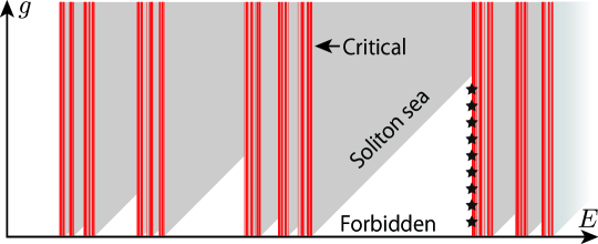
Figure 4: (color online) The spectral structure which consists of the Cantor spectrum of critical states (vertical red lines), the sea of stationary solitons (gray), and the forbidden region, $\tilde{\Gamma_{\infty}}$ (non-colored), in $E$-$g$ plane with the periodic boundary condition. An example of a region where experimentally detectable critical states exist are marked as stars.

6 Phase diagram of the energy spectrum

Let us describe the spectral properties of the nonlinear Schrödinger equation (1) in the limit $\ell\!\rightarrow\!\infty$. A schematic phase diagram is shown in Fig. 4. It consists of three portions, the Cantor set for the critical states, the forbidden region $\tilde{\Gamma}_{\infty}$, and the soliton sea. From the numerical results, we confirm that there exist critical states with the finite coupling $g$ (Fig. 3 (b)). Combining this with Theorem 2, the Cantor set for the critical states is shown as vertical (red) lines in Fig. 4. We numerically found solitons due to the nonlinear effects (Fig. 2 (d)). The point spectrum of the solitons must be distributed outside the forbidden region $\tilde{\Gamma}_{\infty}$ from Theorem 1 and 3. We cannot exclude the possibility that an eigenenergy of a soliton lies just on the Cantor set. It is obvious that surface states are absent with the periodic boundary condition, and not shown in Fig. 4.

7 Summary and conclusion

We studied the stationary states for the nonlinear Schrödinger equation on the Fibonacci optical lattice. We found that the nonlinearity does not destroy the critical states which exist in the absence of nonlinearity and exhibit fractal properties. The existence of these states was confirmed numerically using multifractal analysis. To our knowledge, this kind of analysis is applied to the field of BEC for the first time. We also showed that the energy spectrum of the critical states remains intact irrespective of the strength of the nonlinearity. Besides the critical states, there is a large number of localized solutions, solitons, resulting from the nonlinearity. These solitons may seem an obstacle to observing critical states. However, we found the forbidden region for solitons, in the neighborhood of which the experimental detection of critical states is expected to be possible. Our analysis is intended to stimulate such an experimental effort to observe exotic critical states in optical lattices.

The nonlinear Schrödinger equation (1) is nothing but the discrete Gross-Pitaevskii equation for BEC. Therefore, the chemical potential $\mu$ is equal to some eigenenergy $E$. In real experiments, the controllable parameters are the total number of the particles and the coupling constant $g$. In the nonlinear Schrödinger equation (1), these two parameters appear as a single parameter $g$ which is the effective coupling constant under a normalization condition of the wavefunctions. Within a mean field approximation for many-body BEC systems, the effective single-body state which has the lowest internal energy is most likely to be realized as the ground state. We numerically checked, for relatively small effective couplings $g$ (up to $1$), that the ground state is given by the eigenstate of (1) with the lowest eigenenergy $E$. Then, $E$ is identical to the corresponding the chemical potential $\mu$. When a chemical potential $\mu$ is given instead of the total number of the particles, we can also numerically determine the internal energy.

The method presented in this paper equally applies to a higher dimensional model in which the on-site potential in each direction is arranged by a generic quasiperiodic rule such as the Fibonacci rule. Actually, the eigenstates for the corresponding linear Schrödinger equation have a product form of the one-dimensional eigenstates. (See, for example, [34, 35, 36].) This implies that, in order to detect critical states or fractal wavefunctions on BEC, experimentalists do not necessarily need to stick to a one-dimensional system. Also our method is applicable to a wide class of nonlinear Schrödinger equations for studying the properties of stationary states. For example, we can treat bichromatic on-site potentials [4] which is considered as the Harper equation [26, 27], two different hopping integrals arranged in the Fibonacci sequence [8, 32], and different types of nonlinearities such as the Ablowitz-Ladik one [37].

Appendix A Nonlinear effects for localization

Although Theorem 4 below holds for a wide class of nonlinear Schrödinger equations which have a localization regime in the spectrum of the corresponding linear Schrödinger equation, we consider a random nonlinear Schrödinger equation in one dimension as a concrete example. The nonlinear Schrödinger equation is given by replacing the on-site Fibonacci potential with a random potential in (1). As is well known, all the eigenstates in the corresponding linear system are localized for a general class of randomness in one dimension. As to the nonlinear eigenvalue problem, a certain set of localized eigenstates is proved to exist for more general setting [23, 24, 25]. See also a related article [39].

In the following, we will prove that there is no stationary solution of the nonlinear Schrödinger equation such that the solution exhibits conventional properties of critical or extended states. Unfortunately, we cannot exclude the existence of certain pathological states which are not localized. We believe that such pathological states cannot appear for standard systems. Thus, the localization of the stationary states are expected to survive switching on the nonlinearity [40]. Clearly, our result is consistent with the previous results[23, 24, 25].

Let $\{\Lambda(k)\}_{k=1}^{\infty}$ be a sequence of finite lattices satisfying

$$\Lambda(1)\subset\Lambda(2)\subset\cdots\subset\Lambda(k)\subset\cdots.$$

Let $\tilde{\bm{\psi}}^{(k)}\!=\!(\tilde{\psi}_{1}^{(k)},\tilde{\psi}_{2}^{(k)},\ldots,\tilde{\psi}_{N(k)}^{(k)})$ be a stationary solution of the nonlinear Schrödinger equation on the lattice $\Lambda(k)$ with the eigenenergy $\tilde{E}^{(k)}$, where $N(k)$ is the number of the sites in $\Lambda(k)$. We choose the sequence $\{\Lambda(k)\}_{k=1}^{\infty}$ so that the eigenenergy $\tilde{E}^{(k)}$ converges to some value ${\tilde{E}}$ in the infinite-volume limit $k\rightarrow\infty$. Set

$$\bm{\phi}^{(k)}:=(\phi_{1}^{(k)},\phi_{2}^{(k)},\ldots,\phi_{N(k)}^{(k)}):=\frac{1}{\max_{i}{|\tilde{\psi}_{i}^{(k)}|}}\tilde{\bm{\psi}}^{(k)}.$$ (25)

For the wavefunction $\tilde{\bm{\psi}}^{(k)}$, we introduce the following two conditions:

$$\lim_{k^{\prime}\rightarrow\infty}\lim_{k\rightarrow\infty}\sum_{i\in\Lambda(k^{\prime})}\left|\phi_{i}^{(k)}\right|^{2}=\infty,$$ (26)

and there exists a finite lattice $\Omega$ such that

$$\mathop{\lim\inf}_{k\rightarrow\infty}\max_{i\in\Omega}\left|\phi_{i}^{(k)}\right|>0.$$ (27)

The former condition (26) implies that the wavefunction $\tilde{\bm{\psi}}^{(k)}$ is not localized, and it does not split into two portions, a localized part and the rest, such that the distance between two portions becomes infinity in the infinite-volume limit. In fact, if

$$\lim_{k^{\prime}\rightarrow\infty}\lim_{k\rightarrow\infty}\sum_{i\in\Lambda(k^{\prime})}\left|\phi_{i}^{(k)}\right|^{2}<\infty,$$ (28)

then $\bm{\phi}^{(k)}$ converges to a localized state in the infinite-volume limit even for a critical or extended state ${\tilde{\bm{\psi}}}^{(k)}$.

The latter condition (27) implies that the wavefunction $\bm{\phi}^{(k)}$ does not disappear from finite regions.

We also consider the corresponding linear Schrödinger equation, and write $H_{0,N(k)}$ for the Hamiltonian. The statement is given in a generic form as follows:

Theorem 4.

Let $\tilde{\bm{\psi}}^{(k)}$ be a stationary solution of the nonlinear Schrödinger equation. Suppose that the eigenenergy ${\tilde{E}}$ in the infinite-volume limit is an interior point of the localization regime in the energy spectrum of the corresponding linear Schrödinger equation. Then the solution $\tilde{\bm{\psi}}^{(k)}$ cannot simultaneously satisfy the above two conditions (26) and (27). In other words, if a stationary solution is purely critical or extended in the sense of (26) and satisfies the energy condition, then its dominant part in the sense of the absolute value of the wavefunction cannot appear in any finite region.

Proof.

Assume that $\tilde{\bm{\psi}}^{(k)}$ satisfies the conditions (26) and (27). From this assumption, we will show that one can construct an extended or a critical state for the corresponding linear Schrödinger equation in the infinite-volume limit.

From (27), there exist a subsequence $\{\Lambda(k_{j})\}_{j=1}^{\infty}$ of $\{\Lambda(k)\}_{k=1}^{\infty}$ and a site $i_{0}\in\Omega$ such that $\phi_{i_{0}}^{(k_{j})}$ converges to some nonzero value $\phi_{i_{0}}^{(\infty)}>0$ as $j\rightarrow\infty$. Therefore, we can obtain a wavefunction $\bm{\phi}^{(\infty)}$ in the infinite-volume limit by using the diagonal trick around the site $i_{0}$. Clearly, the wavefunction $\bm{\phi}^{(\infty)}$ is nonvanishing, and non-normalizable from the condition (26).

In the same way as in (11), we define by $\tilde{H}_{N(k)}$ the Hamiltonian with the additional potential $U$ which is determined by $\tilde{\psi}_{i}^{(k)}$. Then, we have $\tilde{H}_{N(k)}\bm{\phi}^{(k)}\!=\!\tilde{E}^{(k)}\bm{\phi}^{(k)}$.

From these, we have

$$\lim_{j\!\rightarrow\!\infty}\left\langle\chi^{(j)},\tilde{H}_{N(\ell_{j})}\bm{\phi}^{(\ell_{j})}\right\rangle =\left\langle\chi^{(\infty)},H_{0,\infty}\bm{\phi}^{(\infty)}\right\rangle$$

$$=\tilde{E}\left\langle\chi^{(\infty)},\bm{\phi}^{(\infty)}\right\rangle,$$ (29)

where $\{\ell_{j}\}_{j=1}^{\infty}$ is a subsequence of $\{k_{j}\}_{j=1}^{\infty}$, and $\chi^{(j)}$ is a function which converges to a rapidly decreasing function $\chi^{(\infty)}$ in the limit $j\!\rightarrow\!\infty$, and $H_{0,\infty}$ is the Hamiltonian of the linear Schrödinger equation in the infinite-volume limit. This result implies that $\bm{\phi}^{(\infty)}$ is a generalized eigenvector of $H_{0,\infty}$. Since $\bm{\phi}^{(\infty)}$ is non-normalizable, this contradicts with the assumption that $\tilde{E}$ is an interior point of the localization regime. ∎

The result (29) implies that the vector $\bm{\phi}^{(\infty)}=(\cdots,\phi_{-1}^{(\infty)},\phi_{0}^{(\infty)},\phi_{1}^{(\infty)},\cdots,\phi_{i}^{(\infty)},\cdots)$ locally satisfies the linear Schrödinger equation as

$$t\left(\phi_{i+1}^{(\infty)}+\phi_{i-1}^{(\infty)}\right)+V_{i}\phi_{i}^{(\infty)}={\tilde{E}}\phi_{i}^{(\infty)}.$$ (30)

If there exists a localization regime in the corresponding linear Schrödineger equation, then the statement of Theorem 4 generally holds. For example, the Harper model has a localization regime for certain values of the coupling constant of the quasiperiodic potential. Therefore, there is no stationary solution which is a conventional critical or extended state by switching on nonlinearity under the condition that the nonlinear potential $U$ vanishes in the infinite-volume limit. As a result, we can expect that the localization of the stationary states in the model is not destroyed by nonlinearity.

Finally, we remark the following: Localization of stationary states may not lead to dynamical localization for nonlinear systems. (For related articles, see [42, 16, 17, 18, 19, 20, 21].) However, the existence [23, 24, 25] of stationary localized states implies that, if nonlinearity dynamically destroys localization in a linear system, whether a wavefunction is dynamically localized or not strongly depends on the initial wavefunction. Actually, if an eigenstate is localized as a stationary solution of the nonlinear Schrödinger equation, then the time evolution of the state is localized, too.

References

References

- [1] Bloch I 2005 Nat. Phys. 1 23
- [2] Morsch O and Oberthaler M 2006 Rev. Mod. Phys. 78 179
- [3] Fallani L, Lye J E, Guarrera V, Fort C and Inguscio M 2007 Phys. Rev. Lett. 98 130404
- [4] Larcher M, Dalfovo F and Modugno M 2009 Phys. Rev. A 80 053606
- [5] Bakr W S, Gillen J I, Peng A, Folling S and Greiner M 2009 Nature 462 74
- [6] Kohmoto M, Kadanoff L P and Tang C 1983 Phys. Rev. Lett. 50 1870
- [7] Ostlund S, Pandit R, Rand D, Schellnhuber H J and Siggia E D 1983 Phys. Rev. Lett. 50 1873
- [8] Kohmoto M, Sutherland B and Tang C 1987 Phys. Rev. B 35 1020
- [9] Penrose R 1974 Bull. Inst. Math. Appl. 10 266
- [10] Gardner M 1977 Sci. Am. 236 110
- [11] Sütő A 1989 J. Stat. Phys. 56 525
- [12] Levi L, Rechtsman M, Freedman B, Schwartz T, Manela O and Segev M 2011 Science 332 1541
- [13] Johansson M and Riklund R 1994 Phys. Rev. B 49 6587
- [14] Kohmoto M and Oono Y 1984 Phys. Lett. A 102 145
- [15] Kivshar Y S and Agrawal G P 2003 Optical Solitons: From Fibers to Photonic Crystals. Academic Press, London
- [16] Pikovsky A S and Shepelyansky D L 2008 Phys. Rev. Lett. 100 094101
- [17] Wang W M and Zhang Z 2009 J. Stat. Phys. 134 953
- [18] Flach S, Krimer D O and Skokos Ch 2009 Phys. Rev. Lett. 102 024101
- [19] Skokos Ch, Krimer D O, Komineas S and Flach S 2009 Phys. Rev. E 79 056211
- [20] Fishman S, Krivolapov Y and Soffer A 2009 Nonlinearity 22 2861
- [21] Krivolapov Y, Fishman S and Soffer A 2010 New J. Phys. 12 063035
- [22] Fishman S, Krivolapov Y and Soffer A 2012 Nonlinearity 25 R53
- [23] Albanese C and Fröhlich J 1988 Commun. Math. Phys. 116 475
- [24] Albanese C, Fröhlich J and Spencer T 1988 Commun. Math. Phys. 119 677
- [25] Albanese C and Fröhlich J 1991 Commun. Math. Phys. 138 193
- [26] Harper P G 1955 Proc. Phys. Soc. Sec. A 68 874
- [27] Aubry S and Andrè G 1980 Ann. Isr. Phys. Soc. 3 133
- [28] Manela O, Segev M, Christodoulides D N and Kip D 2010 New J. Phys. 12 053017
- [29] Halsey T C, Jensen M H, Kadanoff L P, Procaccia I and Shraiman B I 1986 Phys. Rev. A 33 1141
- [30] Kohmoto M 1988 Phys. Rev. A 37 1345
- [31] Hiramoto H and Kohmoto M 1992 Int. J. Mod. Phys. B 3 281
- [32] Fujiwara T, Kohmoto M and Tokihiro T 1989 Phys. Rev. B 40 7413
- [33] Reed M and Simon B 1978 Methods of modern mathematical physics: Vol. IV: Analysis of operators. Academic Press, New York
- [34] Ueda K and Tsunetsugu H 1987 Phys. Rev. Lett. 58 1272
- [35] Schwalm W A and Schwalm M K 1988 Phys. Rev. B 37 9524
- [36] Ashraff J A, Luck J-M and Stinchcombe R B 1990 Phys. Rev. B 41 4314
- [37] Ablowitz M J and Ladik J F 1976 J. Math. Phys. 17 1011
- [38] Lifshits I M, Pastur L A and Gredeskul S A 1988 Introduction to the theory of disordered systems. Wiley, New York
- [39] Fröhlich J, Spencer T and Wayne C E 1986 J. Stat. Phys. 42 247
- [40] McKenna M J, Stanley R L and Maynard J D 1992 Phys. Rev. Lett. 69 1807
- [41] Gel’fand I M and Vilenkin N Y 1968 Generalized functions: Vol. 4: Applications of harmonic analysis. Academic Press, London
- [42] Bourgain J and Wang W M 2007 Diffusion Bound for a Nonlinear Schrodinger Equation. In Mathematical aspects of nonlinear dispersive equations. Princeton Univ. Press