Fu Ori outbursts and the planet-disc mass exchange

Abstract

It has been recently proposed that giant protoplanets migrating inward through the disc more rapidly than they contract could be tidally disrupted when they fill their Roche lobes $\sim 0.1$ AU away from their parent protostars. Here we consider the process of mass and angular momentum exchange between the tidally disrupted planet and the surrounding disc in detail. We find that the planet’s adiabatic mass-radius relation and its ability to open a deep gap in the disc determine whether the disruption proceeds as a sudden runaway or a balanced quasi-static process. In the latter case the planet feeds the inner disc through its Lagrangian L1 point like a secondary star in a stellar binary system. As the planet loses mass it gains specific angular momentum and normally migrates in the outward direction until the gap closes. Numerical experiments show that planet disruption outbursts are preceded by long “quiescent” periods during which the disc inward of the planet is empty. The hole in the disc is created when the planet opens a deep gap, letting the inner disc to drain onto the star while keeping the outer one stalled behind the planet. We find that the mass-losing planet embedded in a realistic protoplanetary disc spawns an extremely rich set of variability patterns. In a subset of parameter space, there is a limit cycle behaviour caused by non-linear interaction between the planet mass loss and the disc hydrogen ionisation instability. We suggest that tidal disruptions of young massive planets near their stars may be responsible for the observed variability of young accreting protostars such as FU Ori, EXor and T Tauri stars in general.

1 Introduction

Young protostars can be highly variable (e.g., Herbig, 1989). The best known members of this club are the Fu Orionis objects, which are young stars showing very large (factors of hundreds) and abrupt increases in their brightness (Hartmann & Kenyon, 1996). Observations of these objects are best understood as variability in the accretion rate onto the growing protostar from a base accretion rate state of $\sim 10^{-7}{\,{\rm M}_{\odot}}$ yr^-1 to a high of up to $10^{-4}{\,{\rm M}_{\odot}}$ yr^-1. Although detailed statistics is still lacking, the duration of the outbursts is believed to be in the range of tens to hundreds of years. Clear spectroscopic signatures implicate an accretion disc in the inner $\lower 2.15277pt\hbox{$\;\buildrel<\over{\sim}\;$}1$ AU as the driver of this variable accretion rate and luminosity output (Zhu et al., 2007; Eisner & Hillenbrand, 2011). The rise times of the outbursts are very short, from a year to $\sim$ ten years. FU Ori phenomenon is not just a fine detail of young stars evolution: the statistics of FU Ori objects suggests that an average proto-star may experience 10-20 of such outbursts, which may still be considered a lower limit on the importance of the FU Ori outbursts (Hartmann & Kenyon, 1996). It is not impossible that proto-stars accrete most of its mass during these relatively short but very intense growth episodes.

A rather natural model for FU Ori variables is a viscously and thermally unstable accretion disc that undergoes periodic switching between the stable quiescent and the outburst states (e.g., Bell & Lin, 1994). Hydrogen is mainly neutral in the quiescent state and is mainly ionised in the outburst state, partially explaining the large difference in the accretion rates. In detail, however, external triggering of the outbursts may still be desirable (e.g., Bonnell & Bastien, 1992; Bell et al., 1995; Lodato & Clarke, 2004), as the theoretically produced outburst rise time scales are longer than $\sim$ 10 yrs.

The key deficiency of the pure thermal disc instability model (e.g., Bell & Lin, 1994) is in the fact that the unstable inner disc region is relatively small, e.g., $R\sim 20{\,R_{\odot}}\sim 0.1$ AU (Zhu et al., 2007). This produces outbursts that are too short, unless one uses very small values for the viscosity $\alpha$-parameter, e.g., as small as $\alpha=10^{-4}$ (Lodato & Clarke, 2004). This seems to be unlikely (King et al., 2007; Zhu et al., 2009). In addition, spectral modeling of the inner disc of the FU Ori variables (Zhu et al., 2007), and their NIR interferometry Eisner & Hillenbrand (2011), require the hot disc region to be greater than $R\sim 0.5-1$ AU, which is clearly too large for the pure thermal disc instability models (Zhu et al., 2009). The small extent of the unstable region translates into too small a disc mass participating in the instability (since the mass is set by the critical surface densities at which the instability operates; Bell & Lin, 1994). The disc instability model thus may be said to suffer from the “mass and time-scale deficit problem” as there is not enough mass in the disc to explain the observed long and bright FU Ori outbursts.

A very promising way forward to enlarging the unstable region, and thus solving the deficit problem, was proposed by Armitage et al. (2001). These authors pointed out that the intermediate disc region, $R\sim 0.1-2$ AU is expected to have a layered structure (Gammie, 1996). The disc midplane region is shielded by the upper layers from the ionisation sources, and is likely to be too cold to support the Magneto-Rotational Instability (e.g., Balbus & Hawley, 1998) that would otherwise yield an efficient angular momentum transport. Accretion thus proceeds only inside the upper ionised “skin” of the disc. Bulk of the material is underneath the skin, too cold to flow radially, settling into what is called “the dead zone”. Over time, and in the right range of external mass supply rates, the dead zone becomes very massive, e.g., $\sim 0.1{\,{\rm M}_{\odot}}$, which eventually triggers a gravitational instability. The associated gravito-turbulence (Lin & Pringle, 1987; Rice et al., 2005) initiates a rapid angular momentum transfer. Armitage et al. (2001) obtained relatively bright, $\dot{M}\sim 10^{-5}{\,{\rm M}_{\odot}}$ yr^-1, outbursts lasting for as long as $10^{3}-10^{4}$ yrs. The current consensus is that the model of Armitage et al. (2001) satisfies observational and physical constraints on FU Ori outbursts better than any other (e.g., Zhu et al., 2009).

Here we propose another solution to the inner disc mass deficit problem, which relies on an entirely different mass reservoir. We suggest that the material accreted onto the star during the FU Ori outbursts comes from giant young planets that fill their Roche lobes inside the inner 1 AU from the star. The planets are assumed to be pushed inward closer to the star by gravitational torques of the protoplanetary disc. The significance of young planets as serious contenders on the role of mass donors for FU Ori outbursts is easily appreciated. The mass of gaseous proto-planets may be as high as tens of Jupiter masses ($M_{J}$), much higher than the likely disc mass in the inner fractions of an AU. If the material of such a planet is dumped into the inner disc and then accreted onto the star at an accretion rate of $\sim 10^{-4}{\,{\rm M}_{\odot}}$ yr^-1, then there is enough gas for a $\sim O(100)$ yrs-long accretion outburst.

Our work is based on ideas of Nayakshin (2011b) who pointed out that the early ($t\lower 2.15277pt\hbox{$\;\buildrel<\over{\sim}\;$}1$ Myr) stages of the thermal relaxation of the planet are highly uncertain and model dependent (see a fuller discussion of this in §3.4). The “low density start” models of such planets are sufficiently fluffy to be tidally disrupted inside a fraction of an AU. We shall also find important connections to the earlier work of Lodato & Clarke (2004) who showed that a massive planet in the inner disc region can trigger rapid rise outbursts, as observed. Finally, our calculations of young protoplanet disruptions are complimentary to the “outburst accretion mode” simulations of large ($10-1000$ AU) discs by Vorobyov & Basu (2005, 2006). These authors have found that massive gaseous clumps born in their discs at $\sim O(100)$ AU distances migrate inward quickly, being accreted by their inner boundary condition.

The purpose of our paper is to investigate the process of tidal disruption of compact proto-planets in the inner $\sim 0.1$ AU of the star in unison with a more self-consistent modeling of the protostellar disc evolution to probe the proposed link of young protoplanets to the FU Ori outbursts. To model the disc, we use the standard (Shakura & Sunyaev, 1973; Frank et al., 2002) 1D time-dependent viscous disc evolution equations in the presence of a massive embedded satellite. An approximate but well understood and tested type II migration model is used to communicate the gravitational torques between the planet and the disc (Lin & Papaloizou, 1986; Lodato & Clarke, 2004). In our modeling of the mass loss, we are aided by the well known results from semi-detached stellar binaries (e.g., Ritter, 1988).

The structure of the paper and main results are the following. In §2 we build a simplified analytical theory for the mass loss and radial motion of the planet embedded in a proto-planetary disc. We show that due to conservation of angular momentum, a mass-transferring planet may migrate outward. Repeating the well known stellar binary results, we also find that the mass transfer rate and the migration pattern can be a quasi-steady or run-away process that may end in a complete (or nearly so) destruction of the planet. We introduce our numerical methods in §3. In §4 we present numerical experiments in which the outer disc is replaced by a constant external torque parameter. This allows us to test our simplified theory in a “clean” controlled setting. In §5, simulations with a self-consistent disc evolution and torque on the planet are presented. A range of variability patterns is found there, and further expanded on in §6. The effective temperature profiles of our disc models are discussed in §7. In §8 we summarise the main results of our paper.

2 Analytical considerations

The numerical scheme presented in §4 is well suited for studying tidal disruptions of planets in arbitrarily initialised time-dependent gas discs. Here we attempt to build a simple analytical understanding of what to expect from numerical simulations later on. We start with the simplest possible situations and gradually add different physical effects. In this section, the outer accretion disc is only considered as a source of a given gravitational torque on the planet ($\tau_{e}$, cf. §2.3) affecting its radial motion. The inner disc interaction with the planet is described by the parameter $f_{a}$ introduced shortly below. We emphasise that $\tau_{e}$ and $f_{a}$ are only defined for convenience of our analytical study (this section); these parameters are replaced by a self-consistent treatment of the disc-planet torques in the time-dependent numerical calculation.

2.1 Outward radial migration driven by planet’s mass loss

A planet embedded in an accretion disc is a subject to gravitational torques from the surrounding discs that in general push it inward (Lin & Papaloizou, 1979; Goldreich & Tremaine, 1980). Here we point out that a mass-losing planet can push itself outward. Operationally, the effect is due to a different balance between the inner and the outer disc torques than that in the standard no-mass-loss case; however, the effect is best understood simply on the basis of angular momentum conservation in the star-planet system.

Consider a planet of mass $M_{p}$ orbiting the star of mass $M_{*}\gg M_{p}$ at a distance $a$ in a circular orbit. The planet’s orbital angular momentum is given by

$$J_{p}=M_{p}\Omega_{a}a^{2}=M_{p}\left(GM_{*}a\right)^{1/2}\;.$$ (1)

If the planet fills its Roche lobe and transfers mass inward through the Lagrangian L1 point (Frank et al., 2002), the system is analogous to a semi-detached stellar binary system with an extreme mass ratio. In the case of conservative mass transfer, we have $dM_{*}/dt=-dM_{p}/dt>0$. We neglect the spin angular momentum of the planet as it is small compared to the orbital angular momentum. We first assume that the star’s spin does not change as a result of gas accretion onto it, in which case the planet’s angular momentum is conserved during the mass transfer process. Therefore,

$${d\ln a\over dt}=-2{d\ln M_{p}\over dt}\;.$$ (2)

This demonstrates that the planet migrates outward as it loses mass. This effect is well known in stellar binary evolution where a conservative mass exchange between the two components leads to widening of the orbit if the secondary is less massive than the primary, and shrinking of the orbit if mass is lost by the more massive star (Ritter, 1988).

In a more general case, accretion of mass onto the star may spin up the star. Alternatively, the star could be slowing down its rotation by passing angular momentum to the inner disc via magnetospheric torques (Collier Cameron & Campbell, 1993; Armitage & Clarke, 1996). Also, as we shall see later, the angular momentum of the gas accreting onto the star may flow past the planet’s orbit if the gap, which is generally opened in the disc by a massive planet, is closed. If the viscous time of the inner disc is long compared with the planet’s mass loss timescale, then we should also account in equation 2 for the angular momentum stored in the disc. To continue with our analytical arguments below, we find it convenient to introduce a free parameter describing the efficiency of the outward migration due to mass transfer, $f_{a}>0$:

$${d\ln a\over dt}=-2f_{a}{d\ln M_{p}\over dt}\;.$$ (3)

If the star is a sink of angular momentum, $f_{a}<1$, but if it gives the angular momentum to the disc then $f_{a}$ may be larger than unity.

We emphasise that, while introduced for convenience in the analytical considerations described here, $f_{a}$ is not a free parameter of our numerical simulations (see Section 3 below), since the outward torque on the planet due to the inner disc is calculated self-consistently. We only use $f_{a}$ in our analytical model below, and also for an interpretation of the numerical results in cases where we can make a good guess on the appropriate value of $f_{a}$.

2.2 Planet’s mass loss rate

Mass transfer from a Roche lobe-filling secondary to the primary has been a subject of numerous papers in the context of cataclysmic binaries secular evolution (e.g., Ritter, 1988). The main result of these studies is that the mass loss rate is a very strong function of $\Delta r=r_{p}-r_{H}$, where

$$r_{H}=a(M_{p}/3M_{*})^{1/3}$$ (4)

is the Hills radius of the planet, which we set approximately equal to its Roche lobe radius, and $r_{p}$ is the planet’s radius. The mass loss rate is very small for negative $\Delta r$, increasing rapidly for positive $\Delta r$.

These basic facts are in fact sufficient for the analytical treatment below, but we find it timely to introduce our numerical mass transfer scheme here as well, to emphasise the importance of the difference $\Delta r$ once more. Before the Roche lobe of the secondary is filled, $\Delta r<0$, the mass transfer rate has an exponential form reflecting the exponential decrease of density with height in the stellar atmosphere (cf. eq. 9 of Ritter, 1988):

$${dM_{p}\over dt}=-{\rho_{\rm ph}c_{\rm ph}r_{H}h_{p}\over e^{1/2}}\exp\left[{\Delta r\over h_{p}}\right]\;,$$ (5)

where $h_{p}$ is the scale height of the planet’s atmosphere, $\rho_{\rm ph}$ and $c_{\rm ph}$ are the photosphere’s density and sound speed, respectively.

When the Roche lobe of the planet is filled, and $\Delta r>0$, the mass transfer rate can be calculated in a similar way (see section 1 of Pringle & Wade, 1985), and the result turns out to be dependent on whether the outer layers of the star are convective or radiative (Rappaport et al., 1983; Kolb & Ritter, 1992). For an isothermal atmosphere, $dM_{p}/dt\propto\exp[\Delta r/h_{p}]$, with $h_{p}=$const, whereas for a convective star with polytropic index $\gamma$, the result is

$${dM_{p}\over dt}\propto-\Delta r^{(3\gamma-1)/(2(\gamma-1))}\;\quad\hbox{if}\quad\Delta r>0\;$$ (6)

(equation (1.27) in Pringle & Wade, 1985). Importantly, for any value of $\gamma>1$ this function is strongly increasing with $\Delta r$. For $\gamma=5/3$, for example, $dM_{p}/dt\propto-\Delta r^{3}$, whereas for molecular hydrogen, $\gamma\approx 1.4$, and $dM_{p}/dt\propto-\Delta r^{4}$. For definitiveness, we parametrise the mass flow rate through the L1 point as

$${dM_{p}\over dt}=-\left({\Delta r\over r_{p}}\right)^{3}{M_{p}\over t_{\rm dyn}}\;\quad\hbox{if}\quad\Delta r>0\;,$$ (7)

where $t_{\rm dyn}=\sqrt{r_{p}^{3}/GM_{p}}$ is the (internal) dynamical time of the planet. Note that when the planet fills its Roche lobe, $t_{\rm dyn}\approx 1/\Omega_{k}(a)=\sqrt{GM_{*}/a^{3}}$, and we can re-write equation 7 as

$${dM_{p}\over dt}=-2{\,{\rm M}_{\odot}}\;\mbox{yr}^{-1}a_{0.1}^{-3/2}\;{M_{p}\over 10M_{J}}\;\left({\Delta r\over r_{p}}\right)^{3}\;,$$ (8)

where $a_{0.1}=a/$(0.1 AU). Since the headline factor in equation 8 is so large, one obtains very high Roche lobe overflow rates even for modest values of $\Delta r$. For example, even at $\Delta r=0.01r_{p}$ the overflow rate is about two order of magnitude larger than the mean accretion rate onto embedded protostars, $\dot{M}\sim 10^{-8}{\,{\rm M}_{\odot}}$ yr^-1 (Hartmann et al., 1998).

We found through experimenting with different power-law indexes in this dependence that the results are very insensitive to the exact form of the mass loss rate dependence on $\Delta r$. This result is well known from stellar binary evolutionary calculations, and will be re-derived for the problem at hand below. Physically, since the mass transfer rate is a strong function of $\Delta r$, it turns out that the process is stable only if $|\Delta r|$ may be maintained very small, which is equivalent to requiring $r_{p}\approx r_{H}$. In this situation the mass loss rate self-adjusts to satisfy the angular momentum loss or gain constraints (cf. Ritter, 1988). Different mass loss formulations only yield slightly different values of $\Delta r$ at which the required equilibrium value of $dM_{p}/dt$ is achieved.

On the other hand, in cases where the mass transfer leads to $r_{H}$ shrinking faster than $r_{p}$, or $r_{p}$ increasing faster than $r_{H}$, a runaway mass transfer occurs. One well known example of this in stellar binaries is the case where the secondary is more massive than the primary, in which case the separation of the components shrinks rather than increases as the mass is transferred (Pringle & Wade, 1985). In this case the disruption of the companion is nearly dynamical, and therefore the exact form of the transfer rate is again not very important.

2.3 Roche lobe overflow: L1 or both L1 and L2?

We follow here the usual assumption that the planet’s surface is determined by the equipotential surfaces (e.g., §of Frank et al., 2002). We also assume that the planet and the star are on circular orbits around the centre of mass of the system. The dimensionless potential in a frame corotating with the centre of mass of the star-planet system has two saddle points, L1 and L2. The points lie on the line connecting the star and the planet, with L1 positioned between the planet and the star, and L2 further away “behind” the planet.

In stellar binaries, the overflow of the secondary’s Roche lobe always proceeds via the Lagrangian point L1 since it is much closer to the secondary. However, for the planet-star system, the mass ratio, $q=M_{p}/M_{*}$, is very small, and thus the overflow may proceed via both L1 and L2. We quantify this following the treatment given in §4.1 of Gu et al. (2003). The difference between distances of the L1 and L2 points ($D_{1}$ and $D_{2}$, respectively) from the centre of the planet are

$$\Delta D\equiv D_{2}-D_{1}\approx{2\eta a\over 3}\left(\eta^{1/2}+\eta\right)\;,$$ (9)

where $\eta=r_{H}/a=(M_{p}/3M_{*})^{1/3}\ll 1$ (see eq. 63 in Gu et al., 2003).

We see that the point L2 is distance $\Delta D$ further away from the centre of the planet than L1. Now, if the atmosphere’s scaleheight $h_{p}$ were infinitely small, the overflow would only proceed via the L1 point (if the planet overflow maintains the $r_{p}=r_{H}\approx D_{1}$ condition). However, if the atmosphere is extended enough, that is $h_{p}\lower 2.15277pt\hbox{$\;\buildrel>\over{\sim}\;$}\Delta D$, then the outflow should proceed through both points L1 and L2.

Equation (66) of Gu et al. (2003) shows that

$${h_{p}\over\Delta D}\approx{9\over 8}\;{c_{\rm ph}^{2}a\over GM_{p}}\;.$$ (10)

Our models will characteristically assume that $T_{\rm eff}\sim 10^{3}$ K (see §3.4 below), and the planet-star separation at which the Roche lobe overflow occurs is often $a\sim 0.1$ AU. For these fiducial parameters,

$${h_{p}\over\Delta D}\approx 0.45\;\left({T_{\rm eff}\over 10^{3}\;\mbox{K}}\right)\;\left({a\over 0.1\mbox{AU}}\right)\;\left({M_{J}\over M_{p}}\right)\;.$$ (11)

This shows that for massive young protoplanets, $M_{p}\sim 10M_{J}$, the overflow should indeed proceed mainly via the L1 point, but as the planet’s mass drops below $1M_{J}$ both L1 and L2 can be letting the planet’s atmosphere to escape.

There is actually one further condition to check. In §2.2 we have shown that the overflow rate is a strongly increasing function of $\Delta r$. In the simulations below, we shall find relatively large Roche lobe overflow rates, requiring small but not infinitesimally small values for $\Delta r/r_{p}$. The difference between locations $L1$ and $L2$, $\Delta D$, is also small in units of $r_{p}$. For a large enough values of $|dM_{p}/dt|$, it is possible that the required Roche lobe “overfilling”, $\Delta r$, is larger than $\Delta D$. We expect that if $\Delta r\lower 2.15277pt\hbox{$\;\buildrel<\over{\sim}\;$}\Delta D$, the overflow proceeds mainly via L1 as argued above, but if $\Delta r\gg\Delta D$, both L1 and L2 will siphon gas away at comparable rates. To compare these, we note that for $M_{p}=10M_{J}$, $\Delta D\approx r_{p}\eta^{3/2}=0.06r_{p}(M_{p}/10M_{J})^{1/2}$. On the other hand, the planet mass loss of $|dM_{p}/dt|=10^{-4}{\,{\rm M}_{\odot}}$ yr^-1 requires $\Delta r\approx 0.037r_{p}$. Thus we see that, at least for $M_{p}=10M_{J}$ the overflow should proceed mainly through the L1 point.

In general, the ratio of the two length scales is

$${\Delta r\over\Delta D}\approx 0.6\;\left[{|dM_{p}/dt|\over 10^{-4}{\,{\rm M}_{\odot}}\mbox{yr}^{-1}}\right]^{1/3}\;a_{0.1}^{1/2}\left({10M_{J}\over M_{p}}\right)^{-5/6}\;.$$ (12)

This shows that at the high mass loss rates the outflow proceeds via L1 point as long as $M_{p}\lower 2.15277pt\hbox{$\;\buildrel>\over{\sim}\;$}5M_{J}$; at lower planet masses the outflow may occur via both L1 and L2 points.

We conclude that in the most typical parameter space sampled by our models below, the Roche lobe overflow occurs via the L1 point. However, for relatively low mass planets, $M_{p}\lower 2.15277pt\hbox{$\;\buildrel<\over{\sim}\;$}1M_{J}$, the overflow should take place via both L1 and L2. In this paper we make an approximation that the outflow always occurs via L1.

2.4 Definitions

The time evolution of $\Delta r$ is of primary interest to us here. Let us calculate the full time derivatives of the Hill (Roche) radius and the planet radius:

$${d\ln r_{H}\over dt}=\left({\partial\ln r_{H}\over\partial\ln M_{p}}\right){d\ln M_{p}\over dt}+\left({\partial\ln r_{H}\over\partial t}\right)_{\dot{M}_{p}=0}\;,$$ (13)

and

$${d\ln r_{p}\over dt}=\left({\partial\ln r_{p}\over\partial\ln M_{p}}\right){d\ln M_{p}\over dt}+\left({\partial\ln r_{p}\over\partial t}\right)_{\dot{M}_{p}=0}\;,$$ (14)

respectively. Here, $(\partial\ln r_{p}/\partial\ln M_{p})$ is the adiabatic mass-radius exponent of the planet, discussed below, and $(\partial\ln r_{p}/\partial t)_{\dot{M}_{p}=0}$ is the time derivative of planet’s radius due to thermal relaxation, e.g., radiative cooling of the planet. Similarly, $(\partial\ln r_{H}/\partial\ln M_{p})$ is the rate of Hills radius change due to planet’s mass changing, and $(\partial\ln r_{H}/\partial t)_{\dot{M}_{p}=0}$ is the term due to external torques onto the planet in the absence of the mass loss.

Since $r_{H}=a(M_{p}/3M_{*})^{1/3}$, and in view of equation 3,

$$\zeta_{H}\equiv{\partial\ln r_{H}\over\partial\ln M_{p}}\approx-2f_{a}+1/3\;,$$ (15)

where we neglected the small term $-(\partial\ln M_{*}/\partial\ln M_{p})=q=M_{p}/M_{*}\ll 1$. Further, we introduce the following notations for brevity

$$\zeta_{p}\equiv{\partial\ln r_{p}\over\partial\ln M_{p}}\;,$$ (16)

$$\tau_{c}=\left({\partial\ln r_{p}\over\partial t}\right)_{\dot{M}_{p}=0}^{-1}\;,$$ (17)

$$\tau_{\rm e}=\left({\partial\ln r_{H}\over\partial t}\right)_{\dot{M}_{p}=0}^{-1}=\left({\partial\ln a\over\partial t}\right)_{\dot{M}_{p}=0}^{-1}\;.$$ (18)

The mass-radius relation for a polytropic planet is given by

$$r_{p}\propto M_{p}^{\frac{1-n}{3-n}}\;,$$ (19)

where $n=1/(\gamma-1)$ is the polytrope’s index, and $\gamma$ is the ratio of the specific heats for the planet’s gas. It is noteworthy that the radius-mass relation for a polytrope strongly depends on $\gamma$, and that the polytropic cloud usually (for large enough values of $\gamma$) expands as the mass is lost. For example, for $\gamma=5/3$, $n=3/2$, and $r_{p}\propto M_{p}^{-1/3}$; for $\gamma=7/5$, $n=5/2$, $r_{p}\propto M_{p}^{-3}$.

Note that $\tau_{\rm e}$ can be related to the external torque, $T_{\rm ext}$, on the planet. Here we anticipate that in our model situation the external torque is negative, $T_{\rm ext}<0$, pushing the planet closer to the star. To relate $\tau_{\rm e}$ and $T_{\rm ext}$, note that angular momentum conservation in the absence of mass loss yields

$$M_{p}{d\over dt}\left(GM_{*}a\right)^{1/2}=-|T_{\rm ext}|\;,$$ (20)

where $(GM_{*}a)^{1/2}=\Omega_{a}a^{2}$ is a specific angular momentum of the planet. From which we conclude that

$$\tau_{\rm e}^{-1}=-{2|T_{\rm ext}|\over M_{p}\Omega_{a}a^{2}}<0$$ (21)

Note also that $\tau_{\rm c}$ is negative for a planet contracting as the result of radiative cooling and it is positive for a planet expanding with time at a constant mass. The latter situation may occur when the planet’s interior is heated by the solid core accretion luminosity (Pollack et al., 1996; Nayakshin, 2011a), or due to dissipation of tides induced by the parent star (e.g., Gu et al., 2003), irradiation (Burrows et al., 2000; Baraffe et al., 2003).

2.5 Stability of mass transfer

In accord with our plan to progress from simple to more complex we first study a non-cooling planet without external torques, i.e., $1/\tau_{\rm e}=1/\tau_{c}=0$, which has $R_{H}\approx R_{p}$, i.e., transfers mass onto the star at some non-zero rate, $-\dot{M}_{p}^{(0)}$. As far as realistic planets in massive gas discs are concerned, this model situation is of an academic interest, as one needs external torques or internal evolution of the planet (e.g., planet swelling due to internal or tidal heating) to fill its Roche lobe, but it will be seen to provide important hints to the results of the more realistic numerical experiments later on.

Following the discussion in §2.2, the dominant factor in the mass loss rate dependence is the difference $r_{p}-r_{H}$. Write

$${d\ln M_{p}\over dt}\approx-\phi\left(\Delta r\right)\;,$$ (22)

where $\phi>0$ is a positive and monotonically increasing function of its argument (note that $dM_{p}/dt<0$). We have explicitly neglected here the much slower dependence of the mass transfer rate on other variables (such as the photosphere’s temperature and the density in equation 5). Within this approximation, we have,

$${d^{2}\ln M_{p}\over dt^{2}}=-\phi^{\prime}\left({dr_{p}\over dt}-{dr_{H}\over dt}\right)\;,$$ (23)

where $\phi^{\prime}=\partial\phi/\partial\Delta r$. Since at the onset of the mass transfer $r_{p}\approx r_{H}$,

$${d^{2}\ln M_{p}\over dt^{2}}=-\phi^{\prime}r_{p}\left({d\ln r_{p}\over dt}-{d\ln r_{H}\over dt}\right)\;.$$ (24)

Referring now to equations 13, 14, and definitions 15, 16, we find that

$${d^{2}\ln M_{p}\over dt^{2}}=-\phi^{\prime}r_{p}\left(\zeta_{p}-\zeta_{H}\right){d\ln M_{p}\over dt}\;.$$ (25)

It is now apparent that the stability of the mass transfer rate is determined by the sign of $\zeta_{p}-\zeta_{H}$ since $\partial\phi^{\prime}>0$. If this term is negative, the mass loss rate increases exponentially with time. Thus, the mass loss is unstable if

$$\zeta_{p}-\zeta_{H}=\zeta_{p}-{1\over 3}+2f_{a}<0\;,$$ (26)

where we used equation 15. This relation demonstrates that stability of the mass loss process is decided by the mass-radius relation for the planet, and by the angular momentum transfer between the planet and the star (the factor $f_{a}$). Physically, this is because the planet moves outward as the result of the mass transfer, which increases $r_{H}$. However, the planet may also increase in size due to mass loss. When the condition (26) is satisfied, $r_{p}$ increases faster than $r_{H}$ as the planet siphons away its mass. In this case, once the planet filled its Roche lobe (Hill’s radius), the mass loss process is a runaway one.

The opposite situation, $\zeta_{p}-\zeta_{H}>0$, is stable. In the presently considered case of zero external torques and no cooling, the mass loss rate drops exponentially with time. The physics of this is simple – the planet moves outward and eventually it becomes smaller than its Roche lobe. In a more realistic situation where there are non-zero external torques, a steady-state situation can be set up, where the planet moves radially at just the right rate to maintain the balance $r_{p}\approx r_{H}$.

Clearly, the stability of the mass transfer is strongly dependent both on the details of the evolution of the planet’s angular momentum (described by the parameter $f_{a}$) and by the evolution of the planetary radius in response to mass loss (described by the parameter $\zeta_{p}$).

2.6 Quasi equilibrium mass loss

Let us now turn our attention to more realistic situations where the external torque and the planet’s radius internal evolution are not negligible. In this case equation 24 leads to

$${d^{2}\over dt^{2}}\ln M_{p}=-\phi^{\prime}r_{p}\left[\left(\zeta_{p}-\zeta_{H}\right){d\ln M_{p}\over dt}+{1\over\tau_{c}}-{1\over\tau_{\rm e}}\right]\;.$$ (27)

Since this is a linear differential equation, our conclusions about the stability of mass transfer do not change. If $\zeta_{p}-\zeta_{H}<0$, the mass transfer is unstable as the mass loss rate runs away exponentially.

However, if $\zeta_{p}-\zeta_{H}>0$, there is a quasi steady state solution of the above equation with $d^{2}\ln M_{p}/dt^{2}\approx 0$, where the mass loss rate is locked at a unique value given by

$$\dot{M}_{\rm eq}=-{M_{p}\over\zeta_{p}-\zeta_{H}}\left({1\over\tau_{c}}-{1\over\tau_{\rm e}}\right)\;.$$ (28)

This result, except for different notations, is the same as equation (16) of Ritter (1988), a well known result in the binary mass transfer studies.

We note that if the planet is cooling and there is no internal energy source, then $\tau_{c}<0$, e.g., the planet contracts with time (equation 17). The external torque is also negative by assumption, therefore for a contracting planet,

$$\dot{M}_{\rm eq}=-{M_{p}\over\zeta_{p}-\zeta_{H}}\left(-{1\over|\tau_{c}|}+{1\over|\tau_{\rm e}|}\right)\;.$$ (29)

As $\dot{M}_{p}<0$ by definition, we see that the quasi-equilibrium mass loss solution is possible only if $|\tau_{c}|>|\tau_{e}|$. In the opposite case the planet contracts too quickly to be tidally disrupted (Nayakshin, 2011b); despite migrating in closer to the star, the mass transfer rate shuts down with time because $r_{p}$ decreases faster than $r_{H}$.

On the contrary, if there are evolutionary reasons for the planet to swell with time, such as stellar irradiation or a powerful internal energy release by the solid core, then the thermal relaxation term in equation 28 amplifies rather than dumps the mass loss rate. In fact, mass loss from the planet may occur in this case even if there are no external torques on the planet.

We can now justify our claim (also well known from the stellar binary mass transfer studies) in the end of §2.2 that the equilibrium mass transfer rate does not depend on the exact form of the mass transfer rate function, $\phi$. As long as that dependence is monotonic and a strong one, the difference $\delta r=r_{p}-r_{H}$ adjusts to “the right value” which yields the equilibrium mass transfer rate given by equation 28. The mass transfer rate in this sense is not a “driving” variable of the problem; it is one determined by the balance of the torques on the planet.

Curiously, in the case of the external torques strongly dominating over the thermal relaxation of the planet, $|\tau_{\rm e}|\ll|\tau_{c}|$, the mass transfer rate is further insensitive even to the planet’s mass, $M_{p}$. Consulting equation 21, we find that equation 28 reads in this case,

$$\dot{M}_{\rm eq}=-{2|T_{\rm ext}|\over\zeta_{p}-\zeta_{H}}{1\over\Omega_{a}a^{2}}\;.$$ (30)

That is, in this case, the mass loss rate depends only on the external torque and location of the planet, $a$, but not the mass of the planet.

2.7 Radial migration due to mass loss

Having understood the conditions under which the mass transfer rate can be steady, we now turn to the consequences of this for the radial migration of the planet. Adding the external torque on the planet to equation 3, we have

$${d\ln a\over dt}=-2f_{a}{d\ln M_{p}\over dt}+{1\over\tau_{\rm e}}\;.$$ (31)

When the mass loss rate is in the steady state regime (equation 28), this becomes

$${d\ln a\over dt}={1\over\tau_{\rm e}}{\zeta_{p}-1/3\over\zeta_{p}-1/3+2f_{a}}+{1\over\tau_{\rm c}}{2f_{a}\over\zeta_{p}-1/3+2f_{a}}\;.$$ (32)

We remind ourselves that $\tau_{\rm e}$ is defined to be negative (equation 21), that is, the the external torques are defined to drive the planet in rather than out. In contrast, $\tau_{\rm c}$ could be positive or negative. The remarkable property of equation 32 is that, depending on the different terms in the equation, the planet may migrate either in or out despite being pushed inward by the external torque, e.g., the outer disc. Furthermore, the relative magnitude of these terms may vary as the planet loses mass or evolves internally. We shall later see that due to this, the same planet may change the direction of migration several times.

2.7.1 Negligible cooling: inward or outward migration?

When the thermal evolution of the planet is insignificant during the tidal disruption process, so that $|\tau_{c}|\gg|\tau_{e}|$, we can neglect the cooling term in equation 32:

$${d\ln a\over dt}={1\over\tau_{\rm e}}{\zeta_{p}-1/3\over\zeta_{p}-1/3+2f_{a}}\;.$$ (33)

Recall that in the steady-state mass transfer rate regime, the denominator of equation 33 is positive (cf. §2.5). Since $\tau_{e}<0$, we see that when the polytropic approximation for the planet is adequate,

$$\hbox{sign}\left({da\over dt}\right)=-\hbox{sign}\left(\zeta_{p}-1/3\right)\;.$$ (34)

That is, the planet migrates outward if $\zeta_{p}<1/3$, and inward otherwise. In particular, polytropic planets that expand as they lose mass ($\zeta_{p}<0$) always migrate outward. Physically, $\zeta_{p}$ controls the amount of mass that the planet has to shed in response to being forced inward by the external torque. This response is meager for planets that shrink due to mass loss. In order to maintain the $r_{p}\approx r_{H}$ equilibrium condition, such planets may simply lose mass as $r_{H}$ shrinks. Thus external torques are able to push these planets in. In the opposite case, when $\zeta_{p}<0$, applying the external torque to push the planet in causes it to lose so much mass that the outward torque of this material exceeds the originally applied torque, and the planet thus moves outward rather than inward.

2.7.2 Rapidly cooling planets

When thermal relaxation of the planet is not negligible, e.g., $|\tau_{c}|$ comparable to or much smaller than the external torque time scale, $|\tau_{e}|$, the last term in equation 32 cannot be neglected. A casual look at the equation 32 would suggest that a rapidly contracting planet, $\tau_{c}<0$, $|\tau_{c}|\ll|\tau_{e}|$, migrates as prescribed by the last term of that equation. However, as remarked after equation 29, the quasi-equilibrium mass loss is only possible if $|\tau_{c}|>|\tau_{e}|$ or else the rapid thermal contraction of the planet shuts down the mass transfer entirely because $r_{p}$ becomes smaller than $r_{H}$.

Nevertheless, even in the quasi-equilibrium situation the second term in equation 32 may indeed exceed the first one and hence dictate the direction of the planet’s migration. To give an example, consider our standard case of a planet with $\zeta_{p}=-1/3$ (gas polytropic index $\gamma=5/3$). Equation 32 reads for this case

$${d\ln a\over dt}=-{1\over\tau_{\rm e}}{1\over 3f_{a}-1}+{1\over\tau_{\rm c}}{3f_{a}\over 3f_{a}-1}\;.$$ (35)

Therefore we see that for $|\tau_{c}|$ somewhat larger than $|\tau_{e}|$, the planet may lose the mass in the quasi-steady regime and yet migrate outward if $f_{a}$ is sufficiently close to unity.

2.7.3 Thermally expanding planets

Let us now turn to the case of planets expanding as the result of thermal evolution, e.g., an inner energy source such as the solid core formation due to dust sedimentation (Nayakshin, 2011a). By definition, $\tau_{\rm c}>0$ in this case, so the steady-state mass loss is possible for any value of $\tau_{\rm e}$ (provided $\zeta_{p}-\zeta_{H}>0$). The last term in equation 32 acts to push the planet outward; however, depending on the first term in that equation the migration direction can be inward or outward.

3 Numerical Methods

3.1 Mass and angular momentum transfer in the disc

We use the code of Lodato et al. (2009) for the evolution of an accretion disc in the presence of an embedded satellite, rescaled to the case of a protostar of mass $M_{*}$ and a planet of mass $M_{\rm p}$. The disc is described by a diffusive evolution model that includes the tidal torque term arising from the planet and the mass deposition term, related to the planet mass loss:

$$\frac{\partial\Sigma}{\partial t} = \frac{3}{R}\frac{\partial}{\partial R}\left[R^{1/2}\frac{\partial}{\partial R}(R^{1/2}\nu\Sigma)\right]-\frac{1}{R}\frac{\partial}{\partial R}\left(2\Omega R^{2}\lambda\Sigma\right)$$ (36)

$$- \frac{\dot{M}_{p}}{2\pi R}\;\delta\left(R-R_{\rm dep}\right)\qquad$$

where $\lambda=\Lambda/(\Omega R)^{2}$, and $\Lambda$ is the specific tidal torque, where

$$\lambda= \displaystyle\frac{q^{2}}{2}\left(\displaystyle\frac{a}{p}\right)^{4} R>a$$ (37)

$$\lambda= -\displaystyle\frac{q^{2}}{2}\left(\displaystyle\frac{R}{p}\right)^{4} R<a.$$

In equation (37), $\Omega=\sqrt{GM_{*}/R^{3}}$ is the angular velocity at radius $R$, $a$ is the radial position of the planet, $q=M_{p}/M_{*}$ and $p=R-a$. This simplified form of the specific torque is commonly used in literature (see, e.g., Lin & Papaloizou 1986; Armitage & Bonnell 2002; Lodato & Clarke 2004; Alexander et al. 2006). We smooth the torque term for $R\approx a$, where it would have a singularity (see equation 37). We use the same smoothing prescription as in Syer & Clarke (1995) and Lin & Papaloizou (1986), i.e. for $|R-a|<\max[H,r_{H}]$, where $H$ is the disc thickness and $r_{H}=a(M_{\rm p}/3M_{*})^{1/3}$ is the size of the Hill sphere (Roche lobe) of the planet.

We shall note here that we use a constant $\alpha$-viscosity parameterisation for the angular momentum transfer in the disc. Gravitoturbulent discs could in principle generate an additional viscosity through gravitational torques (Lin & Pringle, 1987; Gammie, 2001; Rice et al., 2005). However, here we are interested in the inner few AU discs that are unlikely to be self-gravitating since the radiative cooling is very inefficient in units of local dynamical time in such discs (e.g., Rafikov, 2005; Clarke & Lodato, 2009). Such small discs are also expected to be much less massive than the central star and hence the global model of mass transfer is also very unlikely (Lodato & Rice, 2005; Cossins et al., 2009).

The last term in equation 36 describes the mass deposition in the inner disc by the planet (note that $\dot{M}_{p}<0$). The mass deposition takes place into a narrow ring centred onto the deposition radius $R_{\rm dep}$, which is the circularisation radius of the planet’s material lost through the L1 point into the inner disc. The specific angular momentum of the gas at L1 is $\Omega_{a}(a-r_{H})^{2}$, where $\Omega_{a}=\sqrt{GM_{*}/a^{3}}$, and thus the deposition radius is given by

$$R_{\rm dep}=a\left(1-\frac{r_{H}}{a}\right)^{4}\;.$$ (38)

Operationally, we find the radial zone inside of which $R_{\rm dep}$ fall and deposit all of the mass lost by the planet there. Note that $R_{\rm dep}$ is a function of time. Depositing gas in a single zone does not appear to lead to any numerical problems as the gas spreads in both directions from that locations fairly quickly, resulting in a well behaved surface density profile.

3.2 Thermal disc equations

The rest of disc equations follow the standard vertically-averaged approach (e.g., Shakura & Sunyaev, 1973) with minimum necessary complexity. In particular, disc viscosity in the $\alpha$-prescription for a gas–pressure–dominated disc is

$$\nu=\alpha c_{\rm g}^{2}/\Omega,$$ (39)

where $c_{\rm g}=kT_{\rm c}/\mu m_{H}$ is the gas sound speed at the disc midplane, $T_{\rm c}$ is the midplane temperature, $\mu$ is the dimensionless mean molecular weight and $m_{H}$ is the mass of the proton. The disc vertical scale height $H$ is found by solving for the vertical pressure balance, taking into account the radiation pressure (although for most cases considered here radiation pressure is generally negligible):

$$P_{\rm gas}+{1\over 3}a_{\rm rad}T_{\rm c}^{4}=\frac{GM_{*}}{R}\rho_{c}\left({H\over R}\right)^{2}\;,$$ (40)

where $\rho_{c}$ and $P_{\rm gas}=\rho_{c}kT_{\rm c}/\mu m_{H}$ are the gas midplane density and pressure, respectively, and $a_{\rm rad}$ is the radiation energy density constant. The central gas density and the disc surface density are related by $\Sigma=2\rho_{c}H$.

The midplane equilibrium temperature is solved assuming the vertical energy balance for the disc:

$$\frac{9}{8}\nu(T_{\rm eq})\Sigma\Omega^{2}={\sigma_{B}T_{\rm eq}^{4}\over\tau}\;,$$ (41)

where $\tau=\kappa(\rho_{c},T_{\rm eq})\rho_{c}H$ is the disc opacity for the opacity coefficient $\kappa(\rho_{c},T_{\rm eq})$. For opacities varying slowly with temperature, this approach is entirely satisfactory, as the thermal equilibrium is established on the time scale $t_{\rm th}=1/\alpha\Omega$, which is much shorter than the disc viscous time (e.g., cf. Frank et al., 2002).

We modify this standard equation to account approximately for the irradiation heating of the disc by the star, whose luminosity is set to $L_{*}={\,L_{\odot}}(M_{*}/{\,{\rm M}_{\odot}})^{3}$. The incidence angle of the irradiation for simplicity is set to give $\cos i=0.1$ everywhere, although in principle this should be a function of position and the disc vertical scale height, $H(R)$. Thus we write

$$T_{\rm irr}=\left({L_{*}\cos i\over 4\pi\sigma_{B}R^{2}}\right)^{1/4}\;,$$ (42)

and

$$T_{\rm eq}^{4}=T_{\rm irr}^{4}+\frac{9}{8\sigma_{B}}\tau\nu\Sigma\Omega^{2}\;.$$ (43)

For protostellar discs, however, due to a strong temperature dependence of opacity coefficient $\kappa$ on temperature (primarily), the disc may be thermally unstable (e.g. Bell & Lin, 1994). In terms of equation 43, it means that there may be more than one solution for a given $\Sigma$, and that some of the solutions may be thermally unstable. The time evolution of the disc in this case depends on its previous thermal state, and one needs to solve a time-dependent version of the energy equation rather than assume thermal equilibrium.

While thermal instabilities are clearly relevant to the problem at hand, we would like to concentrate here on the “new” physics – the planet tidal disruption and the resulting inner disc refilling – as much as possible. We therefore pick a very simple and transparent numerical method to deal with thermal instabilities in the present paper. In this minimalist approach, similar to that of Lodato & Clarke (2004), we use a time-dependent energy balance equation with a radial advection of heat term:

$${\partial T\over\partial t}=-{T-T_{\rm eq}\over t_{\rm th}}-v_{R}{\partial T\over\partial R}\;.$$ (44)

In this equation, $T_{\rm eq}$ is found from equation 43 using the previous timestep value for the gas temperature, $T_{t}$, in the disc opacity calculation, $\kappa(\rho_{c},T_{t})$. The radial velocity $v_{R}$ is given by the following:

$$v_{R}=-\frac{3}{\Sigma R^{1/2}}{\partial\over\partial R}\left[\nu\Sigma R^{1/2}\right]+2\Omega R\lambda\;.$$ (45)

Our simple energy equation allows us to capture the thermal disc instability if it does occur without an excessive associated numerical cost.

3.3 Radial motion of the planet

In our approach, there are two ways in which the angular momentum is passed between the planet and the disc. First of these is due to gravitational torques (the second term on the right hand side of equation 36) and is independent of the instantaneous mass loss rate by the planet. The term represents the back reaction of the disc on the planet’s motion and follows from angular momentum conservation (see Lodato et al., 2009):

$$M_{p}\left(\frac{\mbox{d}}{\mbox{d}t}\Omega_{a}a^{2}\right)_{\rm J} = -\int_{R_{\mathrm{in}}}^{R_{\mathrm{out}}}2\pi\Omega^{2}R^{3}\lambda\Sigma dR$$

$$= -2\pi GM_{*}\int_{R_{\rm in}}^{R_{\rm out}}\lambda\Sigma dR,$$

where the integral is taken over the whole disc surface and $\Omega_{a}$ is the angular velocity of the planet. The subscript “J” indicates that the term arises due to the planet-disc angular momentum exchange.

The second channel for the angular momentum exchange is only present when the planet loses mass to the disc. As explained in §3.1, the disc gains material with the specific angular momentum of the L1 point of the planet. The material is deposited at the respective circularisation radius, $R_{\rm dep}$ (equation 38). The planet’s specific angular momentum thus increases at the rate

$$M_{p}\left(\frac{\mbox{d}}{\mbox{d}t}\Omega_{a}a^{2}\right)_{\rm mass\,loss}=-{\dot{M}_{p}}\left[\Omega_{a}a^{2}-\Omega_{a}(a-r_{H})^{2}\right]\;.$$ (47)

Adding the two terms for the radial migration of the planet, we obtain

$$\frac{\mbox{d}\ln a}{\mbox{d}t} = -\frac{4\pi G}{\sqrt{GM_{*}a}}\int_{R_{\rm in}}^{R_{\rm out}}\lambda\Sigma dR$$

$$- \quad\frac{\dot{M}_{p}}{M_{p}}\frac{2r_{H}}{a}\left(2-\frac{r_{H}}{a}\right)\;.$$

Note that the planet mass loss rate appears directly only in the second term on the right hand side, but it is also indirectly present in the first one. As the planet fills in the inner disc with gas, it changes the disc surface density profile, and therefore the first term on the right as well. This system of equations is thus quite non-linear.

3.4 Planet contraction

In this paper we are only interested in the planets disrupted inside the inner 1 AU of the star. Such disruptions were termed “hot” by Nayakshin (2011b) due to their possible physical links to the “hot” jupiters and lower-mass close-in exoplanets. Only giant planets in which molecular hydrogen has been dissociated into atomic or ionised H are dense enough to venture into this region (see Nayakshin, 2010).

Our isolated constant mass planet model is based on the toy model of Nayakshin (2011b) who assumed that the young planet follows a Hayashi-like track during its early evolution (Graboske et al., 1975). The model gives the radius of the planet, $r_{p}(t)$, at time $t$, as

$$r_{p}^{3}(t)={r_{2}^{3}\over 1+Ar_{2}^{3}t}\;,$$ (49)

where $r_{2}$ is the planet’s radius at the time of the second collapse, and $A=24\pi\sigma_{B}T_{\rm eff}^{4}/(GM_{p}^{2})$, where the effective temperature of the planet, $T_{\rm eff}$ is a free parameter that is fixed for a given simulation. To accommodate a range of possible cooling rates, Nayakshin (2011b) explored models of contracting planets with three values of the effective temperature, 500, 1000 and 2000 K, but we test only the mid range model here.

The initial radius of the planet, $r_{2}$, right after molecular hydrogen dissociation is also uncertain, with results depending on dust opacity, internal energy liberation by a possibly present solid core, planet rotation, and the detailed equation of state at high densities (cf. Marley et al., 2007). Following Nayakshin (2011b), we estimate the initial (post-collapse) radius of the planet by the energy conservation argument. We assume that the change in the gravitational potential energy of the planet, $\approx-GM_{p}^{2}/2r_{p}$, as the planet radius collapses, is mainly used to dissociate H₂ molecules and ionise hydrogen atoms. Molecular hydrogen is completely dissociated after the collapse, whereas the fraction of fully ionised hydrogen, $0\leq X_{i}\leq 1$, is a free parameter of the model that encapsulates the uncertainties pointed out above. Going through this simple logic (cf. Nayakshin, 2011b), we obtain for the initial radius of the planet,

$$r_{2}\approx{GM_{p}m_{H}\over D+2X_{i}{\cal E}}\approx 4.5R_{J}{M_{p}\over M_{J}}{1\over 1+2X_{i}{\cal E}/D}\;,$$ (50)

where $D=4.5$ eV and ${\cal E}=13.6$ are the dissociation energy of hydrogen molecules and the ionisation energy of hydrogen atom, respectively. The lowest starting density models correspond to $X_{i}=0$, whereas $X_{1}=1$ give the densest possible models.

In equation 49 the time $t$ is counted from the time of the second collapse, which we take to be the start time of the simulations presented below. This simple model does not take into account the electron degeneracy pressure. For low density start models, electrons becomes partially degenerate only after $t\lower 2.15277pt\hbox{$\;\buildrel>\over{\sim}\;$}10^{6}$ yrs (e.g., Graboske et al., 1975). We do not run our models for that long in the present paper. For the high density start models, we over-estimate the density of the planet (since the electron degeneracy pressure is neglected), but this becomes important only in the innermost regions of the disc, $R\lower 2.15277pt\hbox{$\;\buildrel<\over{\sim}\;$}0.02$ AU, where the planets are likely to be swallowed by the star anyway. We also neglect the importance of the possible solid core inside the planet. We plan to address these issues in future publications.

In practice, we start our calculations with the planet of a given mass $M_{p}$ right after the second hydrodynamical collapse. The initial planet’s radius, $r_{p}(0)=r_{2}$, is given by equation 50. When the mass loss from the planet commences (cf. §2.2), the planet’s radius is advanced according to equation 14. The right hand side of that equation is the sum of the term due to the planet’s mass loss and the radiative cooling term calculated at a constant planet mass. For our toy cooling model, we have,

$${1\over\tau_{c}}=\left({d\ln r_{p}\over dt}\right)_{\dot{M}_{p}=0}=-{1\over 3}\;Ar_{p}^{3}\;,$$ (51)

where $A=24\pi\sigma_{B}T_{\rm eff}^{4}/(GM_{p}(t)^{2})$, i.e., calculated with the evolved $M_{p}(t)$. For reference,

$$|\tau_{c}|=1.8\times 10^{5}\mbox{ yr}\;\left({M_{p}\over 10M_{J}}\right)^{2}\left({0.01\mbox{ AU}\over r_{p}}\right)^{3}\left({1000\mbox{ K}\over T_{\rm eff}}\right)^{4}\;.$$ (52)

3.5 Parameter $f_{a}$ and the gap in the disc

Our analytical study showed that the outcome of the tidal disruption of a planet strongly depends on the parameter $f_{a}$ that describes the fraction of the specific angular momentum lost through L1 but then regained by the planet due to gravitational torques from the inner disc (cf. equation 3). In numerical experiments below, these torques are calculated self-consistently, so $f_{a}$ is neither needed nor introduced. But it may be quite beneficial to know what an effective value of $f_{a}$ is for a given numerical situation to be able to appeal to the analytical insights.

The simplest situation here is when the planet carves out a deep gap in the disc that stops any significant gas flows across the gap. The outer disc can then be viewed as a source of an external torque onto the planet, and the situation is thus quite analogous to that in a semi-detached stellar binary system. In a binary system, in the conservative mass and angular momentum exchange scenario, the disc transfers mass in and angular momentum out, giving the excess specific angular momentum to the secondary. In our problem, if the star accretes gas with the specific angular momentum of the last circular orbit around the star (which we set for simplicity to $R=R_{*}$), $\sqrt{GM_{*}R_{*}}$, and the planet recovers the rest of the specific angular momentum lost through the L1 point, then

$$f_{a}=1-(R_{*}/a)^{1/2}\;.$$ (53)

If $a\gg R_{*}$, then $f_{a}\approx 1$.

Now, when the gap is partially or completely closed, gas is able to flow past the planet, taking with it the excess angular momentum as well. While details clearly depend on how deep the gap is, we expect that $f_{a}$ becomes smaller as the gap closes, and in fact goes to zero in the limit of no gap.

According to Takeuchi et al. (1996), the planet opens an annual gap in the disc if $M_{p}$ exceeds

$${M_{p}\over M_{*}}>2\alpha^{1/2}\left({H\over R}\right)^{2}\;.$$ (54)

As $H/R\sim 0.1-0.2$, the estimated gap opening mass varies from a sub-Jupiter to a few Jupiter masses depending on the $\alpha$-parameter of the disc. Obviously, various degrees of stellar irradiation and different opacity laws can affect the gap opening through increasing or decreasing the geometrical aspect ratio $H/R$.

4 Tests of planetary destruction

We now present a series of controlled numerical experiments. To focus our attention on the planet only, we do not yet introduce an outer disc. Instead, we express the effects of the outer disc by a fixed torque,

$$\left({d\ln a\over dt}\right)_{\rm ext}={1\over\tau_{\rm e}}\;,$$ (55)

where $\tau_{\rm e}=-250$ yrs for the tests below. Except for the extreme mass ratio, $M_{p}/M_{*}$, the setting of the problem is exactly analogous to that of mass transfer in stellar binaries, where the external torque might be due to the gravitational radiation or magnetic breaking. Such a setup facilitates a straight forward comparison with the analytical theory for the planet migration and Roche lobe overflow developed earlier. However, we shall find “new” behaviour compared with stellar binaries motivated by the disc gap closing (something that never happens for stellar binaries). More self-consistent simulations, those without an external torque and where the outer disc torques the planet in, are to follow in §5.

In this section, the planet initial mass is $M_{p}=10M_{J}$, the initial planet-star separation is $a_{0}=0.25$ AU, the initial planet’s radius, $R_{p}=0.021\mbox{AU}\approx 44R_{\rm J}$, obtained from equation 50 with $X_{i}=0$. The effective temperature of the planet is set to $T_{\rm eff}=1000$ K. We do not allow the planet’s mass to fall below $M_{\rm core}=5{\,{\rm M}_{\oplus}}$, assuming that there is a solid core of that mass inside the planet. This particular assumption only affects the results at the very end of the tidal disruption of the planet. We use Thompson scattering opacity for the disc for simplicity (we shall use a more realistic one for the full disc simulations later on). The inner radius of the computational domain, assumed to equal the stellar radius, is $R_{\rm in}=0.01$ AU, and the outer radius is $R_{\rm out}=4.2$ AU (which is sufficient for these tests as we are only interested in the inner regions). The number of grid zones is $N_{r}=500$, unless otherwise stated.

Table 1 shows the list of the simulations presented in this paper, most important parameter values, respective figure numbers and also the most notable behaviour patterns of the disc or the planet.

4.1 Simulation Ext1

The first run presented, labelled Ext1, is for a disc viscosity parameter $\alpha=0.02$ and the planet radius-mass exponent of $\zeta_{p}=-1/3$.

4.1.1 Evolution of the planet

Figure 1 shows the most interesting characteristics of this simulation. The solid line in the top panel shows the planet’s location, $a$, as a function of time, in units of AU. The dashed curve shows the planet mass in units of $10M_{J}$. The solid curve in the middle panel shows the radius of the planet, $R_{p}$, whereas the dashed curve shows the Hill’s radius. The bottom panel of Fig. 1 presents three mass loss/gain rates: the accretion rate onto the star, the absolute value of the planet mass loss rate, $|\dot{M}_{p}|$, and the analytical prediction for that mass loss rate given by equation 28, shown with the solid, the red dotted and the blue dashed curves, respectively.

The general outcome of the simulation is that the planet spirals in for about 200 years with zero mass loss, until it fills its Roche radius and starts losing mass. The mass lost by the planet is transferred into the disc interior to it. A quasi-steady state is established in which the mass loss by the planet is exactly matched by the mass accreted onto the surface of the star. The inner disc transfers its excess angular momentum back to the planet, producing an outward directed torque on the latter. This reverses the direction of planet’s migration. Losing mass, it is migrating outward, as predicted. The quasi-steady state mass loss cannot last forever as the planet’s mass is finite, and eventually the mass loss runs away, destroying most of the gas component of the planet rapidly (see the spike at around 660 yrs). Only $\sim 0.12M_{J}$ of the gaseous planet survive the disruption in this simple model (see §4.1.3 below).

The blue dashed curve in the lower panel of Fig. 1 shows the predicted mass loss rate given by 28 with $f_{a}$ given by equation 53. We observe that the analytical prediction provides an excellent description of the numerical results starting from the time when the planet fills its Roche lobe, e.g., from time $t\approx 200$ yrs to $t\approx 550$ yrs. During this time the mass loss rate from the planet is matched by the accretion rate of the star. The second marker of this quasi-equilibrium is the fact that the rate of planet’s expansion/contraction due to mass loss and radiative cooling is exactly matched by the corresponding change in the Hill’s radius, so that the two are approximately equal (cf. the middle panel of Figure 1). Note that the radius of the planet increases from $t\approx 200$ to $\approx 400$ yrs, and then decreases until the sharp spike. This change in behaviour is explained by the fact that initially the planet’s radius evolution is controlled by the mass loss, with cooling being negligible. Thus the planet initially expands. After $\approx 400$ yrs, when the planet loses about half of its original mass, the radiative cooling becomes dominant in controlling the planet’s radius evolution. The planet then contracts until the accretion rate spike.

The quasi-equilibrium state of the planet-star system is analogous to that of a semi-detached stellar binary system where the lower mass secondary transfers its mass to the primary. However, after $t\approx 550$ yrs the planet’s mass loss rate stops decreasing with time, flattens off and then increases. The accretion rate onto the star follows the trend, but lagging behind the planet’s mass loss. As we shall see below, this is not a time-delay effect but rather is a signature of a very important effect that does not occur in stellar binaries: the closing of the gap in the disc, due to which the inner disc material may flow past the planet. As the result of this, the planet suffers a nearly catastrophic disruption at $t\approx 660$ yrs.

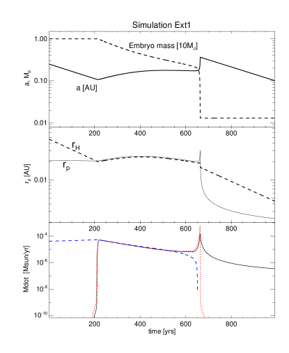
Figure 1: Evolution of a massive gas planet tidally disrupted near its parent star. The top panel shows the radial location and planet’s mass versus time, as labelled. The middle panel shows the planet’s radius, $r_{p}$, and its Hills radius, $r_{H}$. The bottom panel shows the accretion rate onto the star, the planet mass loss rate and the theoretical prediction for that rate (equation 28) with the solid black, red dotted and blue dashed curves, respectively. The theoretical prediction works exceedingly well in the region where the planet fills its Roche lobe and the gap in the disc is opened (see §4.1.1).

4.1.2 Evolution of the disc

Figure 2 shows several snapshots of the disc surface density versus radius covering the most interesting moments of this numerical experiment. The curves are marked by the respective time $t$ shown right next to them. As stated earlier, initially the surface density profile is everywhere zero. At $t\approx 200$ yrs (see the middle panel of Figure 1), the planet eventually fills its Roche lobe and starts transferring mass into the inner disc, filling it out. The first curve shown in Figure 2 corresponds to time $t=198$ yrs (black solid curve), when the planet disruption just begins. The planet at that moment is at $a=0.12$ AU. The material lost through the L1 point is circularised and is deposited at $R_{\rm dep}\approx 0.06$ AU (note the break in the black curve in the Figure), and then spreads viscously in both directions. At small radii the material eventually starts accreting onto the star, whereas at larger radii the torques from the planet prevent it from spreading outwards further. During this time the mass loss rate from the planet exceeds the accretion rate onto the star (the rising part of the red dotted curve at $t\approx 200$ yrs in the bottom panel of Figure 1). The inner disc is thus being filled in by the material lost from the planet.

The swelling of the inner disc cannot go on forever, however. When the mass of the disc becomes significant enough ($t=211$ and $t=219$ yrs curves in Figure 2), the gravitational torque of the inner disc starts to affect the radial migration of the planet. The inner disc torque in fact exceeds that of the externally applied torque and the planet reverses its direction of migration. Migrating outward, it is now able to settle into the self-regulated quasi-steady regime discussed earlier.

This amiable quasi-steady state evolution of the planet and the inner disc continues until time $t\approx 500-600$ yrs or so. By that time, the mass of the planet drops to only $\sim 3M_{J}$. This severely undercuts the ability of the planet to keep the gap open (cf. equation 54). This is why the gap starts to be partially filled by gas, and the material from the inner disc starts to leak into the outer one (cf. the $t=358$ yrs curve in Figure 2). By $t=643$ yrs curve, the gap is seriously compromised. The last of the curves, $t=971$ yrs, shows that in the end the gap is completely erased and the disc spreads viscously outward even more. By that time the planet has lost most of its mass and the disc is hardly aware of its presence (even though it consists entirely from the material formerly belonging to the planet in this simulation).

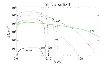
Figure 2: The disc surface density for several different times, as marked on the Figure. The evolution of the disc can be summarised as following: (a) the inner disc is inflated with material from the disrupted planet; (b) the disc pushes the planet outward; (c) the gap is partially closed, leading to a runaway in planet’s mass loss rate; (d) the disc overflows the remaining low mass planet. The evolution after that is that of a “standard” accretion flow unperturbed by the planet.

4.1.3 The late spike/final destruction of the planet

The partial gap closing at $t\sim 600$ yrs has catastrophic consequences for the planet. As the inner disc material diffuses outward through the gap, past the planet’s orbit, less of the inner disc torque is passed on to the planet. In terms of the analytical parameterisation of §2, the fraction of the angular momentum passed back to the planet, $f_{a}$, drops. Since $\zeta_{p}-\zeta_{H}=2(f_{a}-1/3)$ for $\gamma=5/3$ planet, the mass transfer rate from the planet becomes unstable when $f_{a}$ drops below $1/3$. The mass loss rate runs away exponentially at time $t\approx 660$ yrs. Physically, the planet’s radius increases more rapidly due to the mass loss than the Hill’s radius could increase since the outward radial migration is compromised by the leaking gap. As can be seen from the bottom panel of figure 1, during this exponential runaway, the protostellar accretion rate does not manage to keep up with the rate at which the matter is deposited in it. This is not surprising as some of the matter flows outward through the gap.

The runaway planet destruction via Roche lobe overflow is bound to end in one of the two ways. One is a complete unbinding of the gaseous envelope that would leave only a rocky core (which is present for this simulation by assumption). On the other hand, if the cooling time of the planet becomes very short at low masses, the planet may go into a “runaway contraction” phase instead, where it contracts faster than the Hill’s radius expands. This second outcome is indeed what happens in simulation Ext1. The end mass of the planet is $0.12M_{J}$, including the assumed $5{\,{\rm M}_{\oplus}}$ of the rocky core.

We emphasise that the final mass of the planet strongly depends on its internal structure, and so is very model dependent. In our simple constant $T_{\rm eff}=1000$ K cooling prescription, contraction time scale becomes very short at low planet’s masses. This shuts off the mass loss at the end of simulation Ext1. A more realistic cooling model would probably lead to longer cooling times. On the other hand, the solid core may have created its own dense gas “atmosphere” strongly bound to the core, in analogy to the nucleated core instability model for giant planet formation (e.g., Mizuno, 1980; Pollack et al., 1996), as argued by Nayakshin (2011a). This atmosphere is not modelled here, and may remain bound to the core. Clearly, better models of the internal structure of the planets must be used to address the issue of the post-disruption mass.

4.2 Importance of gap opening: simulation Ext2

As we have seen in simulation Ext1, when the gap closes, $f_{a}$ drops since the matter and angular momentum flow from the inner disc into the outer disc, past the planet. This reduces the rate of the outward migration of the planet and may destabilise the mass loss by the planet, leading to its runaway disruption. In view of the gap opening criterion (equation 54), then, the outcome of the planetary tidal disruption depends on the disc viscosity, the planet mass, and the outer disc torque. The latter controls the accretion rate in the inner disc (through the equilibrium mass loss condition in equation 30) which in its turn regulates the geometrical disc aspect ratio, $H/R$.

To explore this issue, we run one further simulation, labelled Ext2, entirely identical to Ext1 except that the viscosity parameter $\alpha$ is increased to $\alpha=0.1$. Figure 3 shows the resulting time evolution of the planet in the same format as Figure 1. The outcome of the higher $\alpha$ simulation is markedly different from that of its lower $\alpha$ counterpart. There is no quasi-steady state plateau in the accretion rate corresponding to an equilibrium tidal evaporation of the planet. Analysis of the disc surface density evolution (not shown here for brevity) for simulation Ext2 shows that there is only a depression in the surface density profile rather than a deep gap. As explained earlier, a partially opened gap lowers the effective $f_{a}$. The planet does not move outwards quickly enough, and the expansion of the planet (recall that $R_{p}\propto M_{p}^{-1/3}$) increases the mass loss rate further, until the planet is destroyed in a runaway fashion.

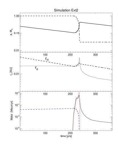
Figure 3: Same as Fig. 1 but for simulation Ext2 with a higher disc viscosity parameter, $\alpha=0.1$. Due to this, the disc is hotter, and the planet is unable to keep the gap opened. As the result, the material from the inner disc is able to flow past the planet. The reduced angular momentum feedback on the planet destabilises the mass transfer process. Most of the planet’s gaseous inventory is completely disrupted on a very short time scale.

4.3 Importance of the mass–radius relation: simulation Ext3

As a final numerical experiment in a series with the fixed external torque timescale, we present simulation Ext3, in which the mass–radius relation for the planet is steeper, $r_{p}\propto M_{p}^{-1}$. That is, $\zeta_{p}=-1$ rather than $-1/3$ for simulations Ext1 and Ext2. Figure 4 shows the outcome of this simulation, demonstrating that there are actually two mass loss episodes and both are unstable.

The stability of the mass transfer depends (see §2.6) on the difference $\zeta_{p}-\zeta_{H}=2f_{a}-4/3$ in this case. If the gap is impenetrable to the gas from the inner disc, and the material lost by the planet is instantaneously gained by the star, then $f_{a}=1-\sqrt{R_{\star}/a}$, as explained in §3.5. The planet is first disrupted at $R\approx 0.11$ AU in this experiment, so $f_{a}\approx 0.7$, and $\zeta_{p}-\zeta_{H}=2f_{a}-4/3\approx 0.1$, i.e., small but marginally positive. However, there is a small lag between the mass loss rate of the planet and the accretion rate, which reduces the effective value of $f_{a}$ below the above (theoretically maximum) estimate. This is probably the reason for the mass transfer being unstable in this simulation.

The first disruption episode is not final in this simulation. As the planet loses all but $\sim 0.3M_{J}$ of its gaseous mass (which corresponds to only 3% of its initial mass), the radiative cooling accelerates, and $r_{p}$ shrinks rapidly. At the same time, the planet migrates outward, so the Hill’s radius increases. This allows the remaining Saturn-mass planet to shut down the mass loss for a while. However, the inner disc drains onto the star, while the “external torque” in our fixed $\tau_{e}$ model continues to push the planet inward. So the planet resumes its inward migration. By the time $t=800$ yrs it finds itself at $R=0.06$ AU, where it fills its Roche lobe for the second time. A second outburst, physically but not quantitatively similar to the first one, results. The remaining reservoir of the gas is lost. The “naked” solid core then continues to migrate inward as prescribed by the fixed $\tau_{e}$ model.

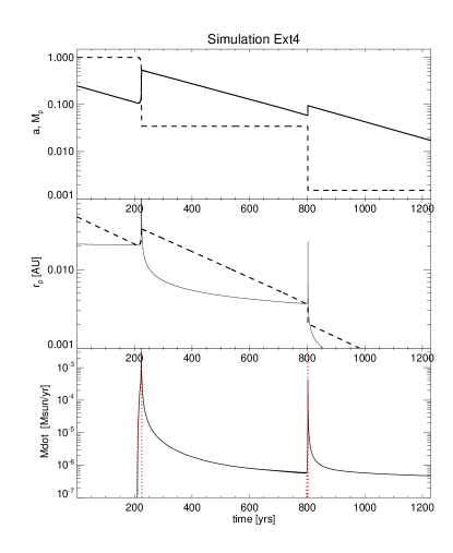
Figure 4: Same as Fig. 1 but for simulation Ext3. Here the mass–radius relation of the planet is steeper, $r_{p}\propto M_{p}^{-1}$. The mass-loss from the planet fuels too fast an expansion of $r_{p}$, so that the difference $r_{p}-r_{H}$ “runs away”, and so does the planet mass loss rate. The planet loses most of its mass on a very short time scale in the first very luminous burst. The remaining gas envelope is unbound in the second disruption when the planet migrates inward even closer.

5 Disruption of planets in realistic discs

5.1 Parameters and initial conditions

We now consider a more realistic set of calculations in which we do not introduce an artificial external torque. Instead, we start with an accretion disc filling in the computational domain. The torque parametrized in §4 by the timescale $\tau_{\rm e}$ is now self-consistently computed from the time-dependent disc structure. The disc is initialised with a surface density profile commonly used in the literature (e.g., Matsuyama et al., 2003; Alexander et al., 2006) in studies of protostellar disc evolution:

$$\Sigma_{0}(R)={A_{m}\over R}\left(1-\sqrt{R_{\rm in}\over R}\;\right)\;\exp\left[-{R\over R_{0}}\right]\;,$$ (56)

where $R_{0}$ is the disc length-scale, set at $R_{0}=5$ AU unless stated otherwise, and $A_{m}$ is a normalisation constant chosen so that the disc contains a given initial mass $M_{d}=2\pi\int_{R_{\rm in}}^{R_{\rm out}}RdR\Sigma_{0}(R)$. In hindsight, the exact shape of the initial surface density profile does not appear very important, as long as one samples all the interesting parameter space by varying other parameters of the problem, such as the disc mass $M_{d}$ and the viscosity parameter $\alpha$. We use the opacity of Zhu et al. (2009) instead of Thompson electron scattering opacity, used in tests Ext1–Ext3. The computational domain is modelled by $N_{r}=500$ to 700 radial zones. We also use $R_{\rm in}=0.02$ AU for the inner boundary of the disc, instead of 0.01 AU as used in tests Ext1–Ext3. The outer boundary of the computational domain is set to $R_{\rm out}=25$ AU for the tests below, or otherwise explicitly stated. We use a reflecting boundary condition at $R_{\rm out}$. This choice is of no particular importance for the results as there is little gas mass at large $R$ and the most interesting effects take place at $R\lower 2.15277pt\hbox{$\;\buildrel<\over{\sim}\;$}1$ AU. In addition, the viscous time at $R_{\rm out}$ is much longer than the duration of the simulations below. The initial mass of the planet is set at $M_{p}=10M_{J}$.

5.2 Simulation Sim1

Simulation Sim1 is done with the following parameters: viscosity parameter $\alpha=0.002$, $M_{d}=20M_{J}$, $X_{i}=0$, $T_{\rm eff}=1000$ K, $\zeta_{p}=-1/3$. The initial location of the planet, $a_{0}=0.13$ AU, is chosen to be such that the Roche radius $r_{H}$ is just slightly larger than the planet radius, $r_{p}$. This is done for computational expediency. Tests Sim3 and Sim4 below are started with larger value for $a_{0}$.

Figure 5 shows the resulting evolution of the planet and the accretion rate onto the star. In brief, the time evolution of the system can be described as the following stages: (i) From $t=0$ to $t\approx 100$ yrs. The evacuation of the disc interior of the planet; (ii) $t\approx 100$ to 400 yrs. An inward migration of the planet and then commencement of the Roche lobe overflow, which re-fills the inner disc; (iii) $t\approx 400$ to 2600 yrs; the quasi steady state outward migration of the planet as the result of the inner disc torque exceeding that of the outer disc torque. The planet loses most of its mass during this time, evolving from $10M_{J}$ to only about $1M_{J}$. (iv) $t\approx 2660$ yrs. The gap is partially closed. This reduces the inner disc torque and destabilises the quasi-equilibrium condition ($r_{p}\approx r_{H}$). The planet mass loss runs away since $r_{p}$ expands faster than $r_{H}$ could increase due to the outward migration. This leads to the “final destruction” spike in the planet mass loss rate (the dotted curve in the bottom panel of figure 5). The planet loses almost all of its gaseous mass in this particular simulation. (v) $t>2660$ yrs, the “post-planet” disc evolution. With the planet now all but destroyed (the remaining solid core is dynamically unimportant for the disc), the disc evolves independently of the planet.

Figure 5: Same as Fig. 1 but for simulation Sim1 that models the disc torques self-consistently.

We now discuss this evolution in greater depth. Figure 6 shows the disc surface density profile at key epochs. Panel (a) concentrates on the earlier times, when the planet is still massive enough to keep the gap opened. The solid curve shows the initial $\Sigma(R)$. The next curve at $t=81$ yrs shows a greatly reduced surface density in the disc interior to the location of the planet. It also demonstrates that the planet pushes the outer disc back, creating a bump in $\Sigma(R)$ just behind the gap. After the inner disc disappears (accretes onto the star), the outer disc pushes the planet closer to the star. Roche lobe overflow sets in, and the inner disc is refilled by the planet’s material. The $t=712$ curve in Figure 6a shows that it is filled almost to the same values of $\Sigma$ as at $t=0$. The planet now migrates outward, and the gap becomes less wide since the planet’s mass is reduced. This description (and Figure 6a) covers simulation stages (i) to (iii), as defined above.

Figure 6b shows what happens when the planet’s mass is too small to keep the gap opened. The gap is significantly compromised by the time of the black solid curve, $t=2654$ yrs. The gap is completely closed, and the planet’s mass is dispersed and assimilated into the inner disc in the next $\sim 20$ yrs (see the $t=2665$ yrs curve). The mass released by the planet streams both inwards – onto the star – and outwards (note the spike in the red $t=2665$ yrs curve in the figure).

Figure 7 zooms in onto the time interval around the “final destruction” of the planet, e.g., around the gap closing, showing the planet’s radius and Hills radius in the top panel, and the accretion rate onto the star (solid) and the planet’s mass loss rate (dotted) in the bottom panel. The planet’s destruction in this simulation ends when only $\approx 0.1{\,{\rm M}_{\oplus}}$ of gas remains bound to the $5{\,{\rm M}_{\oplus}}$ solid core we assumed in this simulation. Given our toy cooling model (fixed $T_{\rm eff}$), this amount of mass cools very quickly, allowing the radius to contract very fast and avoid a complete unbinding of all of the gaseous mass. It is clear that this outcome is completely dependent on the cooling model, which becomes unrealistic at this point. Nevertheless, this demonstrates an important point. If radiative cooling becomes sufficiently rapid as the planet loses mass, the planet (the gas atmosphere of the solid core, actually) may contract below the Hill’s radius before the evaporation of all of the gas. The end result of this is then a solid core plus a gas envelope planet.

We see from Figure 7 that most of the material lost by the planet in the “last disruption” outburst is accreted by the star within half a century or so (see also the curve $t=2831$ yrs in fig. 6b). The disc then evolves independently of the planet, accreting onto the star. The sharp transitions in $\Sigma(R)$ in Figure 6b at late times ($t=6425$ yrs, for example) are caused by the strong opacity jumps where Hydrogen becomes partially ionised.

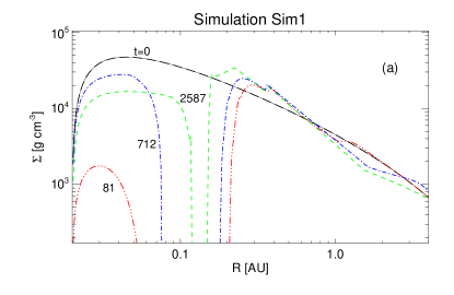
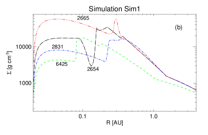
Figure 6: The disc surface density profile for several snapshots from the simulation Sim1. The times of the snapshots are labelled on the figure next to the respective curves. (a) The early evolution of the system. The $t=0$ initial condition neglects the presence of the planet, but the planet opens a gap in the disc very quickly. The inner disc then empties out onto the star. The outer disc then “pushes” the planet closer in where it fills its Roche lobe and starts transferring mass to the inner disc. The inner disc then refills with the planet material. Note that the gap becomes narrower as the planet loses mass. (b) Later evolution of the disc, centred around the spike at $t=2660$ yrs (see Figs. 5 and 7). The planet is rapidly dispersed when the mass loss rate runs away due to the partially closed gap. An ionisation front propagates outward, but stalls quickly. After the giant planet is destroyed, the disc accretes onto the star as if there were no planet.

Figure 7: A zoom in on the evolution of the planet’s radius, and the Hills radius (top panel), and the planet mass loss rate and the star’s accretion rate (the bottom panel) for simulation Sim1.

5.3 Sim1.X: More compact start models

So far we explored only the low density start models, introduced by setting the parameter $X_{i}=0$ (cf. equation 50). This parameter stands for the fraction of the ionised hydrogen atoms in the planet right after the second hydrodynamical collapse. In our toy model for the planet this parameter controls the radius of the planet right after H₂ dissociation. The larger the initial radius of the planet, the farther away from the star can the planet be disrupted. We now explore how the results depend on the value of $X_{i}$, keeping the other parameters of the simulation fixed at same values as in Sim1 (cf. Table 1). We label the simulations Sim1.X, where $X=10\times X_{1}$.

Figure 8 shows the outcome of simulation Sim1.4, with $X_{i}=0.4$. Since the initial radius of the planet is less than one third that of simulation Sim1 (compare the solid curves in the middle panels of Figs. 8 and 5), the planet is able to migrate farther in before it fills its Roche lobe. The planet is located at $R\sim 0.035$ AU at time $t\approx 2300$ yrs when it fills its Roche lobe. In contrast to simulation Sim1, the mass transfer rate is not quasi-steady in this case. The whole of the planet’s envelope is tidally disrupted in a short Roche lobe overflow event. The main destabilising factor is the decreased fractional amount of the angular momentum that the planet receives back when its mass is accreted by the protostar. In particular, $f_{a}=1-\sqrt{R_{\rm in}/a}\approx 0.24$ for the present simulation, whereas for Sim1 $f_{a}\approx 0.55$ due to the more distant disruption location. For $\zeta_{p}=-1/3$, we have $\zeta_{p}-\zeta_{H}=2(f_{a}-1/3)$. Therefore, for simulation Sim1, $\zeta_{p}-\zeta_{H}>0$, whereas for Sim1.4 $\zeta_{p}-\zeta_{H}<0$, explaining the vastly different outcomes of these simulations.

The mass deposited in the inner disc drives the planet outwards to about 0.2 AU. During this short planet Roche lobe overflow spike our model for the mass deposition is probably somewhat unrealistic, as the mass may also overflow through the L2 point, in the outer disc, at these very high outflow rates.

Figure 8: Same as Fig. 5 but for simulation Sim1.4 which differs from Sim1 by a higher hydrogen ionisation parameter, $X_{i}=0.4$. The planet is thus about 3 times more compact, thus being disrupted closer in to the protostar. The disruption is abrupt and non steady because $\zeta_{p}-\zeta_{H}<0$ for this simulation (see §5.3 for detail).

Figure 9 shows the stellar accretion rate evolution near the tidal disruption point for simulations Sim1, Sim1.2, Sim1.3 and Sim1.4. The rise times of the light-curves are between a year to ten, but the more compact the planet is (the larger $X_{i}$), the steeper the rising and the falling parts of the curves. This is natural, as the more compact models are disrupted closer in. The rise time of the light-curves is about the inner disc viscous time, which becomes shorter at smaller values for deposition radius, $R$, scaling as $\propto R^{3/2}$ (at a fixed $\alpha$ parameter and $H/R$).

Figure 9: Comparison of the protostellar accretion rates, $\dot{M}_{*}$, around the first Roche lobe overflow event for simulations Sim1 and Sim1.X. The simulations differ from one another only by the initial ionised hydrogen fraction, $X_{i}=0,0.2,0.3$ and 0.4, for the dashed, solid, dotted and dash-dot curves, respectively. Note that the more compact the planet is (the larger $X_{i}$ is), the shorter the rise time of the outburst and the larger the peak value of $\dot{M}_{*}$. The curves were arbitrarily translated along the time coordinate to appear on the same figure.

5.4 Simulation Sim2: higher disc mass

Figure 10: Same as Fig. 5 but for simulation Sim2. Note that the timescales are shorter and the mass loss rates are larger in Sim2 than they are in Sim1.

We now present simulation Sim2, which is identical to Sim1 except for a higher initial accretion disc mass, $M_{d}=50M_{J}$. Figure 10 shows the main results of this numerical experiment. Since the disc accretion rate is higher, the torques acting on the planet are higher too. Therefore the time scales for planet migration in this simulation are shorter than in Sim1. In terms of our analytical approach to the problem, the external disc torque timescale, $|\tau_{e}|$, is shorter in Sim2 than in Sim1.

As before, the inner disc is first emptied onto the star. The planet fills its Roche lobe at around $t=100$ yrs, starting a very large accretion event. Note that the maximum accretion rate reached in this simulation at the first Roche lobe overflow event is nearly $10^{-4}{\,{\rm M}_{\odot}}$ yr^-1, almost an order of magnitude higher than in simulation Sim1, which is explainable by the larger disc torques onto the planet.

During the quasi-steady Roche lobe overflow stage, the planet migrates outward, as before. Interestingly, by the time it reaches $1M_{J}$ mass, the planet has migrated outward to $R\approx 0.2$ AU, farther than it did in simulation Sim1. This can be understood from equation 32. The two terms on the right hand side of that equation have different signs, with the last term (due to radiative cooling) causing inward migration. This term remains roughly the same in Sim1 and Sim2 as $r_{p}$ is almost the same in the two simulations. However, the external disc torque is much larger in Sim2. Since the net result of the outer disc torque is outward migration in this case, the planet migrates outward faster in Sim2 than it does in Sim1.

We would like to pause here for longer to clarify the physical interpretation of the faster radial migration in Sim2 compared with Sim1 better. At first this result seems to contradict the common sense: “A more massive outer disc should provide a larger spin down torque, so the planet should migrate outward slower or even migrate inward in Sim2 as compared to Sim1”. However, the equilibrium mass loss conditions imply that the planet must lose mass more rapidly in Sim2 precisely because the outer disc torque is larger. This means that the inner disc in Sim2 is more massive than it is in Sim1, and it produces a larger outward torque on the planet. To be in the equilibrium situation, the outward and inward disc torques on the planet must work in such a way as to push it steadily outward at a rate proportional to the outward disc torque (cf. equation 33). So physically, a larger outer disc torque causes a stronger response from the planet through the inner disc feeding and that is why the planet migrates outward even faster.

As the result of this more effective outward migration, the planet does not actually suffers a nearly catastrophic disruption when it reaches $M\approx 1M_{J}$. At the start of the second planet mass loss spike (time $t\approx 400$ yrs in fig. 10), the planet moves outward quickly. Instead of suffering a runaway mass loss as in Sim1, a shutdown of the mass loss occurs at this moment in Sim2. The planet continues to be pushed outward by the inflated inner disc, reaching $R\approx 0.3$ AU at $t\approx 500$ yrs. By that time the inner disc drains sufficiently onto the star, and the inward migration of the planet resumes. Despite some contraction of the planet’s radius with time, the Hills radius becomes smaller than $r_{p}$ again at time $t\approx 800$ yrs. This time Roche lobe overflow is terminal for the gaseous part of the planet, and it is completely destroyed in the third Roche lobe overflow event very quickly. The evolution of the disc after that is similar to Sim1.

5.5 Thermal instability in the gap (Sim3)

To explore the importance of initial conditions, we set up simulation Sim3, which has same initial disc mass as Sim2, $M_{d}=50M_{J}$, but higher disc viscosity parameter, $\alpha=0.01$, and a different disc radial cutoff $R_{0}=7$ AU (see equation 56). The outer boundary of the disc is enlarged to $R_{\rm out}=40$ AU. We also place the planet at larger starting separation, $a_{0}=1$ AU rather than $0.13$ AU in Sim1, Sim2.

The results of this test are shown in Figure 11. If we were to average out the shorter period (tens of years) variations in the curves, the gross evolution of the system is not that different from that found previously. Once again, the inner disc drains onto the star whilst the outer disc is “dammed up” behind the planet. The accretion rate onto the star then plummets to very small values until the planet is pushed to $R\sim 0.11$ AU where it overfills its Roche lobe. The material siphoned from the planet feeds the inner disc, restarting the accretion onto the star. Neglecting the oscillatory pattern for now, the planet loses mass and moves first outward and then inward until $M_{p}\approx 1.5M_{J}$, all the time satisfying $r_{p}\approx r_{H}$. When the gap is partially filled, there is a very large outburst that unbinds the residual gaseous mass of the planet. After this, the gap in the disc shuts completely, and the planet is of no importance for the disc.

Figure 11: Same as Fig. 10 but for simulation Sim3, in which the planet is inserted at $a=1$ AU instead of $a=0.13$ AU. The oscillations in the mass loss/gain rates in the bottom panel are due to thermal ionisation instability in the gap, as explained in §5.5.

However, on shorter time scales, there is far more variability in Sim3 than in any presented before. Figure 12 zooms in onto two selected time intervals from simulation Sim3, showing just the mass loss and accretion rates. An oscillatory behaviour is seen already $\approx 70$ years after the the first Roche lobe overflow (cf. the top panel of fig. 12). Limit-cycle variations persist throughout most of the time preceding the “final destruction spike” (cf. the bottom panel of fig. 12).

Figure 12: Same as the bottom panel of Fig. 11 but zooming onto two interesting time periods in the disc/planet evolution. In the top panel, the beginning of the outburst is shown, when the Roche lobe is overfilled for the first time. The bottom panel of the figure corresponds to the period around the “final” destruction of the gaseous envelope of the planet.

Figure 13 shows the disc central (midplane) temperature, surface density, and the effective temperature, $T_{\rm eff}$, at two times, $t=1171$ yrs, and $t=1195$ yrs. The first of these times (solid black curves in Figure 13) is close to the third peak in the stellar accretion rate curve in the top panel of fig. 12, whereas the second set of curves (red dashed curves in fig. 13, respectively) corresponds to the next trough in the accretion rate.

Concentrating on the top panel of fig. 13, we note that the two curves differ by a factor of $\sim$ two in the inner disc, and are almost identical behind the gap region. However, the gap region is significantly different at these two selected times. In particular, the disc central temperature $T_{c}\sim 2\times 10^{4}$ K at the peak of the accretion rate cycle, and only $T_{c}\sim 800$ K at the minimum of the cycle.

These profound changes in the disc temperature have similarly profound consequences for planet evolution and the inner disc, as that is strongly linked to the planet’s migration and mass loss rate. The middle panel of fig. 13 shows that while the gap is only partially opened at the “high-T” state of the gap region, it gets fully opened at the “low-T” state, when viscosity of the material in the gap drops in response to the temperature variation.

However, what causes the temperature drop in the gap region? To address that, note that the planet mass loss rate actually dips much faster than the stellar accretion rate after any one of the peaks visible in the top panel of 12. This implies that the planet has been pushed outward “too far” by the inner disc torques, and it continues to be pushed even further out for some $\sim 10$ yrs after the peak. The inner disc eventually runs out of material, as it is accreted onto the star. The outer disc then over-powers the torques from the inner one and the planet migrates inward again, restarting the mass loss and re-filling the inner disc for another cycle. Thus, while the gap changes are pronounced, they appear to be driven by the behaviour of the inner disc, which makes the planet to switch between the full-gap to a partial-opened gap states.

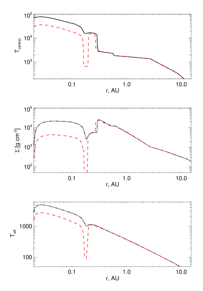
Figure 13: Disc behaviour through one of the instability cycles for simulation Sim3. Top: disc central temperature; Middle: disc surface density; Bottom: disc effective temperature. The curves are for two selected times, $t=1171$ yrs (solid black curves), and $t=1195$ yrs (dashed red curves). These correspond to a peak and a trough in the star’s accretion rate (cf. §5.5).

6 Planet-Disc thermal instabilities

During the outburst state, the inner disc becomes very hot, with most of hydrogen atoms ionised. One may therefore expect that the $\alpha$-parameter may be higher, in accord with estimates from dwarf nova systems King et al. (2007), and Magneto-Rotational Instability simulations (Balbus & Hawley, 1998). Furthermore, modeling of the observations of FU Ori outbursts by Zhu et al. (2007) suggested that $\alpha\sim 0.02-0.2$. We therefore present now simulation Sim4, which is identical to Sim3 except $\alpha=0.04$.

Figure 14: Same as Fig. 14 but for simulation Sim4, which is identical to Sim3 except that $\alpha$-parameter is increased to $\alpha=0.04$. The resulting behaviour change is significant: the thermal disc instability is triggered before the planet overflows its Roche lobe. The resulting disc/planet behaviour is somewhat similar to that found by Lodato & Clarke (2004).

Figure 14 shows the outcome of this simulation, which contains both similarities and also very significant differences from all of the simulations presented earlier. Similarly to the previously studied cases, the inner disc first empties onto the star, while the outer disc pushes the planet in. However, unlike any of the previous cases, the first accretion outburst episode onto the star is not driven by the planet filling its Roche lobe and transferring its mass inward. Instead, at time $t\approx 179$ yrs, thermal disc instability is triggered. At that time, the planet is situated at $R\approx 0.2$ AU and does not fill its Roche lobe.

To analyse the disc behaviour in greater detail, Figure 15 shows the disc structure just before the instability is triggered (black solid curve), during the initial luminosity rise (red dashed curve) and just after the rise (blue dotted). One notices that the instability is actually triggered at the outer banked-up edge of the gap, behind the planet, at $R\sim 0.3$ AU. Before the instability, the disc is relatively cold everywhere, but especially so in the gap. As the instability flares up, the disc behind the gap heats up and the increased pressure of the gas is able to partially close the gap. The gas thus rushes inward, accumulating in the inner disc, sending that region of the disc on the hotter, upper stable branch of the “S-curve” (Bell & Lin, 1994; Lodato & Clarke, 2004), and leading to a massive rapid-rise outburst.

The outburst in the simulation Sim4 is in a qualitative agreement with Lodato & Clarke (2004), except here it is supplemented by the mass loss from the planet. Note that in this high $\alpha$ (and thus high accretion rate) simulation, the mass loss from the planet is a relatively minor detail. Indeed, when the mass loss from the planet sets in ($t\approx 300$ yrs), it exceeds the prior value of the accretion rate onto the star only in the first $\sim 50$ yrs or so. Together with Sim3, this simulation clearly demonstrates that non-linear coupling between the hydrogen ionisation instability in the disc and the planet-disc mass exchange may be important in determining a variability pattern in the accretion rate onto the star.

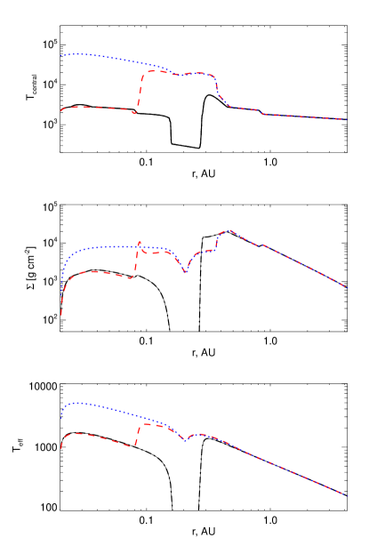
Figure 15: The disc structure at times $t=176.4$ yrs, 179.2 and 179.5 yrs for simulation Sim4, shown with the black solid, red dashed and blue dotted curves, respectively. Note that thermal hydrogen ionisation instability is triggered just behind the gap, and the instability then propagates in, as in models of (Lodato & Clarke, 2004).

7 Emission region size

Figure 16 shows the disc central temperature (top panel) and the disc effective temperature (bottom panel) for several representative times for the simulation Sim4. Along with those curves, we also show the best fit power-laws of the inner hot disc model of Eisner & Hillenbrand (2011) to their NIR Keck interferometer data for the three well known FU Ori objects. These observations have spatial resolution as good as $\sim 0.05$ AU, and thus serve as direct and sensitive probes of the spectral disc model fits.

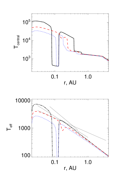
Figure 16: The disc central temperature (Top panel) and the effective temperature (Bottom panel) versus radius for simulation Sim4, at three selected times, $t=1036,1248$ and 1584 yrs, shown with the thick solid black, red dashed and blue dotted curves, respectively. The three black solid power-laws represent the best fitting effective temperature profiles inferred by Eisner and Hillenbrand (2011) for the three FU Ori sources.

The effective temperature profiles of our discs in the inner region are not that dissimilar from the best fit models of Eisner & Hillenbrand (2011), except for the presence of the gap. This qualitative agreement is encouraging, given that we did not try to fine tune our models to satisfy the spectral constraints. This suggests that our models may be relevant to the observed FU Ori sources, although it is desirable to attempt more detailed spectral fits to the observations in the spirit of Eisner & Hillenbrand (2011). This is however beyond the scope of the present paper.

8 Discussion

8.1 Main results of this paper

In this paper we presented calculations of the tidal disruption of massive gaseous planets in massive accretion discs of young protostars. In the analytical part of the paper (§2), we derived conditions under which the mass and angular momentum exchange between the planet and the disc is in a quasi steady state (cf. text around equation 26), and the corresponding equilibrium mass loss rate from the planet. Qualitatively, these conditions require (a) the planet to be massive enough to keep the gap in the disc opened; and (b) the mass-radius relation for the planet to be such that the planet contracts as it loses mass or at least expands only as a weak power-law of the planet’s mass, $M_{p}$.

We then formulated a numerical 1D approach to modeling the planet-disc mass and angular momentum exchange (§3). Utilising a toy cooling model for a young planet, and a fixed external torque driving the planet in, we found that our numerical model reproduces the analytically expected results well (§4), including the quasi-steady state planet’s disruption (Roche lobe overflow), and the eventual closing of the gap and a runaway planet disruption when the planet’s mass becomes too low. We then proceeded to several tests (labelled Sim1 to Sim4 in Table 1) in which the planet-disc torques are calculated self-consistently.

The most robust result of our calculations is that if there is a massive young planet in the inner disc, then the accretion rate onto the protostar must be strongly variable on time scales ranging from a few years to a few hundred or even thousands of years. There are simply too many non linear physical processes occurring in the planet-disc system for the accretion rate to remain static over long time scales.

First of all, as well known from previous literature (Rice et al., 2003) a massive planet opens a deep gap in the disc, blocking the flow of matter from the exterior disc to the inner one. Such a blockade of the protostar by the young planet may be the reason why the average accretion rates of protostars appear to be lower than expected theoretically (Dunham et al., 2010).

We found two ways in which the blockade is ended, and both lead to a rapid rise accretion outburst that may be relevant for the observations of FU Ori outbursts. The first of these, encountered in the relatively high $\alpha$ simulation Sim4 ($\alpha=0.04$, cf. §6 and figure 14), is the same as the Lodato & Clarke (2004) model for FU Ori outbursts. In this case thermal (hydrogen ionisation) instability sets in at the outer edge of the gap in the material piled up behind the planet. Heating up, the outer disc is able to close the gap, overflow the planet and fuel an outside-out accretion outburst.

The second way to kick-start accretion onto the star was found in all of our lower $\alpha$ simulations (Sim1 to Sim3 in Table 1). In these cases the planet is pushed inward sufficiently fast to fill its Roche lobe before the hydrogen ionisation instability at the outer gap takes place. The planet then loses mass through its L1 point. The material circularises inward of the planet, and spreads viscously. As gas accretes onto the protostar, the accretion rate rises by orders of magnitude. What happens next depends on the internal properties of the planet. If conditions for the quasi-steady state mass transfer are satisfied, then the planet migrates radially (usually in the outward direction), so that the Hills radius is exactly equal to the planet’s radius. The resulting outburst light curve may then resemble a step function, similarly to the FU Ori outburst itself (Clarke et al., 2005).

During this quasi-steady state planet-star mass transfer, the role of the planet completely reverses. While before the outburst the planet prevented the material from the outer disc from reaching the star, now it is the donor for the star. Also, like in a stellar binary system, the planet takes the excess angular momentum of the inner disc away and does not allow the material to spread outward viscously. This latter effect keeps the accretion rate onto the star at a higher value for longer than it would have been if the gas could flow past the planet.

If the steady-state conditions for mass transfer are violated, then an even more dramatic outburst may occur. The planet is then tidally disrupted on time scale of a few to few tens of years. The material disrupted off the planet then spreads viscously in both directions, and the accretion rate onto the star drops rapidly as there is no planet to bank up the inner disc in the outward direction.

On the top of this generic behaviour, we found variability on smaller time scales caused by a non-linear connection between the planet migration and mass loss and hydrogen ionisation instability. For example, in simulation Sim3 (§5.5), only the gap region of the disc is unstable and switches between the ionised and the non-ionised states, modulating the accretion rate onto the protostar.

These results do depend quite sensitively on the internal structure of the planet, as we described in §3.4. In particular, if planets are smaller after H₂ dissociation than we assumed in most of our simulations here, then they may not be disrupted at all. In this case the planets are driven all the way into the star or the magnetospheric cavity. This corresponds to the “high density start” models (Nayakshin, 2011b) parametrised by $X_{i}=1$. Therefore, better modeling of the internal relaxation of the growing planets, including possible massive solid cores and the luminosity released by these, is absolutely necessary to detail predictions of our model further.

8.2 Where do the inner planets come from?

It is possible that every young protostar goes through as many as 10-20 FU Ori events during its growth (Hartmann & Kenyon, 1996). Recent modeling of the embedded phase of low mass proto stars by Dunham et al. (2010) also suggests that large amplitude variability in the accretion rate is widespread, and that stars may actually acquire most of its mass in bursts. If our model for FU Ori outbursts is to apply to the observations, many giant planets are required per star. Is this reasonable?

The answer strongly depends on which planet formation theory is accepted. In the standard Core Accretion (CA) model (Pollack et al., 1996; Alibert et al., 2005) of planet formation, giant planets are formed “late”, e.g., after a few Myrs. These planets are also expected to be rather compact (Marley et al., 2007). Tidal disruption of giant CA planets is therefore unlikely, and having as many as ten of such per star would also seem implausible.

The gravitational disc instability model for planet formation (e.g., Boss, 1997) was thought to form planets only at distances greater than 50-100 AU (e.g., Rafikov, 2005) due to inefficient cooling at closer distances (Gammie, 2001; Mayer et al., 2004; Rafikov, 2005; Meru & Bate, 2011). It may therefore appear that planets born at these large distances would be of no relevance to this paper. However, working in the context of proto stellar accretion rather than planet formation, Vorobyov & Basu (2005, 2006) showed that their clumps migrated inward rapidly, reaching all the way to their inner computational domain boundary of 10 AU. These results have been supported by their more recent simulations (Vorobyov & Basu, 2010) and by simulations of a number of independent authors (Boley et al., 2010; Boley & Durisen, 2010; Cha & Nayakshin, 2011; Machida et al., 2011; Baruteau et al., 2011; Michael et al., 2011). Baruteau et al. (2011) provide an in depth analysis of the rapid migration of gas clumps in self-gravitating discs and conclude that these clumps migrate via type I regime. These authors find that massive planets migrate inward faster than a disc gap could be opened. A recently submitted manuscript by Zhu et al (2011b; private communication) also shows many examples of massive clumps migrating inward rapidly although the authors find that some of these clumps become substantially more massive than a giant planet.

Note that these results only apply to the outer gravito-turbulent discs; in the inner non self-gravitating disc regions studied here, planet migration must slow down considerably just because planets we consider are 1-3 orders of magnitude more massive than the total mass of these inner discs. Standard gap opening criteria should apply then.

Boley et al. (2010); Nayakshin (2010) argued that tidal disruption of gaseous envelopes of the giant proto-planets may be a plausible way to form all kinds of planets in what was called the “Tidal Downsizing Hypothesis” for planet formation. More recently, Nayakshin (2011b) have shown that proto-planets in which molecular hydrogen is dissociated are dense enough to undergo tidal disruption inside the inner $\sim 0.1$ AU from the star.

If these ideas are to be relevant to FU Ori outbursts and episodic accretion of stars, one must accept that most early formed planets are completely destroyed and swallowed by their parent stars. This is required both from the fact that many outbursts are needed per star (Hartmann & Kenyon, 1996).

Name${}^{\,a}$	$M_{d}$ ${}^{\,b}$	$\alpha^{\,c}$	$X_{i}$ ${}^{\,d}$	$a_{0}^{\,e}$	$\zeta_{p}^{\;f}$		Figs.${}^{\,g}$	Commentsh
	$\left(M_{J}\right)$			$\left(\hbox{AU}\right)$
Ext1	–	0.02	0	0.25	$-1/3$		1,2	Reference case
Ext2	–	0.1	0	0.25	$-1/3$		3	Gap closed
Ext2	–	0.02	0	0.25	$-1$		4	Unstable mass transfer
Sim1	20	0.002	0	0.13	$-1/3$		5,6, 7	Reference case
Sim1.X	20	0.002	X	0.13	$-1/3$		8,9	closer-in disruptions
Sim2	50	0.002	0	0.13	$-1/3$		10	Temporary shutdown of mass transfer
Sim3	50	0.01	0	1	$-1/3$		11, 12, 13	Thermal instability in the gap
Sim4	50	0.04	0	1	$-1/3$		14	Disc instability before mass loss

Table 1: List of simulations performed and main parameters. Notes:

^a Simulation IDs. Those starting with “Ext” are simulations with an imposed external torque (§4). Those with “Sim” are full disc simulations where the disc-planet torques are calculated self-consistently.

^b Initial disc mass for the full disc simulations.

^c $\alpha$-parameter of the simulation.

^d The fraction of ionised hydrogen used to determine the initial planet radius (eq. 50).

^e The starting location of the planet, in AU.

^f The index of the planet’s mass-radius relation (equation 16).

^g Corresponding figures in the paper.

^h Notable behaviour in the simulation.

9 Conclusions

In this paper we studied the planet and the disc evolution in cases when the young massive gas giant planet overfills its Roche lobe and transfer its mass back into the disc. Due to significant uncertainties in the internal structure of young planets, large parameter space for the problem, and still missing physics, our study cannot yet give definitive answers on what exactly happens with the planets. Instead, this work is to be viewed as one establishing an analytical and numerical framework for further studies of the planet-disc-star mass exchange.

It appears that Roche lobe overflow of young giant gas planets holds a potential promise as an explanation for the enigmatic FU Ori outbursts of protostars. We note in passing that a subset of our models (such as Sim3) may be relevant to shorter period and lower accretion rate variable protostars such as EXors (Herbig, 1989; Sicilia-Aguilar et al., 2008; Lorenzetti et al., 2009). If FU Ori outbursts and episodic accretion onto protostars are indeed connected to tidal disruptions of young planets then the implication would be that many young giant planets are tidally destroyed or perhaps swallowed whole by their parent proto-stars.

Future work should include better treatment of the planet’s internal structure, especially a possible presence of truly massive solid cores, add type I migration (neglected here), the possibility for the overflow through the L2 point (neglected here), and aim to model the “end” result when the gas disc is presumably dispersed by disc photo-evaporation.

10 Acknowledgments

Theoretical astrophysics research in Leicester is supported by an STFC Rolling Grant. This research used the ALICE High Performance Computing Facility at the University of Leicester. Some resources on ALICE form part of the DiRAC Facility jointly funded by STFC and the Large Facilities Capital Fund of BIS. Cathie Clarke’s careful reading of the manuscript and useful suggestions are much appreciated. Andrew King is thanked for discussions of mass transfer in stellar binaries. Richard Alexander is thanked for useful comments on the early draft of the manuscript. Charles Gammie is thanked for showing us the Zhu et al. 2011b manuscript before it appears in the public domain. SN thanks Rashid Sunyaev and the Max Planck Institute for Astrophysics in Garching where the manuscript was completed for hospitality. Finally, we benefited from discussions of planet migration with Sijme-Jan Paardekooper and Clement Baruteau.

References

- Alexander et al. (2006) Alexander R. D., Clarke C. J., Pringle J. E., 2006, MNRAS, 369, 229
- Alibert et al. (2005) Alibert Y., Mordasini C., Benz W., Winisdoerffer C., 2005, A&A, 434, 343
- Armitage & Bonnell (2002) Armitage P. J., Bonnell I. A., 2002, MNRAS, 330, L11
- Armitage & Clarke (1996) Armitage P. J., Clarke C. J., 1996, MNRAS, 280, 458
- Armitage et al. (2001) Armitage P. J., Livio M., Pringle J. E., 2001, MNRAS, 324, 705
- Balbus & Hawley (1998) Balbus S. A., Hawley J. F., 1998, Reviews of Modern Physics, 70, 1
- Baraffe et al. (2003) Baraffe I., Chabrier G., Barman T. S., Allard F., Hauschildt P. H., 2003, A&A, 402, 701
- Baruteau et al. (2011) Baruteau C., Meru F., Paardekooper S.-J., 2011, MNRAS, 416, 1971
- Bell & Lin (1994) Bell K. R., Lin D. N. C., 1994, ApJ, 427, 987
- Bell et al. (1995) Bell K. R., Lin D. N. C., Hartmann L. W., Kenyon S. J., 1995, ApJ, 444, 376
- Boley & Durisen (2010) Boley A. C., Durisen R. H., 2010, ApJ, 724, 618
- Boley et al. (2010) Boley A. C., Hayfield T., Mayer L., Durisen R. H., 2010, Icarus, 207, 509
- Bonnell & Bastien (1992) Bonnell I., Bastien P., 1992, ApJL, 401, L31
- Boss (1997) Boss A. P., 1997, Science, 276, 1836
- Burrows et al. (2000) Burrows A., Guillot T., Hubbard W. B., et al., 2000, ApJL, 534, L97
- Cha & Nayakshin (2011) Cha S.-H., Nayakshin S., 2011, MNRAS, 415, 3319
- Clarke et al. (2005) Clarke C., Lodato G., Melnikov S. Y., Ibrahimov M. A., 2005, MNRAS, 361, 942
- Clarke & Lodato (2009) Clarke C. J., Lodato G., 2009, MNRAS, 398, L6
- Collier Cameron & Campbell (1993) Collier Cameron A., Campbell C. G., 1993, A&A, 274, 309
- Cossins et al. (2009) Cossins P., Lodato G., Clarke C. J., 2009, MNRAS, 393, 1157
- Dunham et al. (2010) Dunham M. M., Evans II N. J., Terebey S., Dullemond C. P., Young C. H., 2010, ApJ, 710, 470
- Eisner & Hillenbrand (2011) Eisner J. A., Hillenbrand L. A., 2011, ArXiv e-prints
- Frank et al. (2002) Frank J., King A., Raine D. J., 2002, Accretion Power in Astrophysics: Third Edition, Accretion Power in Astrophysics, by Juhan Frank and Andrew King and Derek Raine, pp. 398. ISBN 0521620538. Cambridge, UK: Cambridge University Press, February 2002.
- Gammie (1996) Gammie C. F., 1996, ApJ, 457, 355
- Gammie (2001) Gammie C. F., 2001, ApJ, 553, 174
- Goldreich & Tremaine (1980) Goldreich P., Tremaine S., 1980, ApJ, 241, 425
- Graboske et al. (1975) Graboske Jr. H. C., Olness R. J., Pollack J. B., Grossman A. S., 1975, ApJ, 199, 265
- Gu et al. (2003) Gu P.-G., Lin D. N. C., Bodenheimer P. H., 2003, ApJ, 588, 509
- Hartmann et al. (1998) Hartmann L., Calvet N., Gullbring E., D’Alessio P., 1998, ApJ, 495, 385
- Hartmann & Kenyon (1996) Hartmann L., Kenyon S. J., 1996, ARA&A, 34, 207
- Herbig (1989) Herbig G. H., 1989, in European Southern Observatory Conference and Workshop Proceedings, edited by B. Reipurth, vol. 33 of European Southern Observatory Conference and Workshop Proceedings, 233–246
- King et al. (2007) King A. R., Pringle J. E., Livio M., 2007, MNRAS, 376, 1740
- Kolb & Ritter (1992) Kolb U., Ritter H., 1992, A&A, 254, 213
- Lin & Papaloizou (1979) Lin D. N. C., Papaloizou J., 1979, MNRAS, 186, 799
- Lin & Papaloizou (1986) Lin D. N. C., Papaloizou J., 1986, ApJ, 309, 846
- Lin & Pringle (1987) Lin D. N. C., Pringle J. E., 1987, MNRAS, 225, 607
- Lodato & Clarke (2004) Lodato G., Clarke C. J., 2004, MNRAS, 353, 841
- Lodato et al. (2009) Lodato G., Nayakshin S., King A. R., Pringle J. E., 2009, MNRAS, 398, 1392
- Lodato & Rice (2005) Lodato G., Rice W. K. M., 2005, MNRAS, 358, 1489
- Lorenzetti et al. (2009) Lorenzetti D., Larionov V. M., Giannini T., et al., 2009, ApJ, 693, 1056
- Machida et al. (2011) Machida M. N., Inutsuka S.-i., Matsumoto T., 2011, ApJ, 729, 42
- Marley et al. (2007) Marley M. S., Fortney J. J., Hubickyj O., Bodenheimer P., Lissauer J. J., 2007, ApJ, 655, 541
- Matsuyama et al. (2003) Matsuyama I., Johnstone D., Hartmann L., 2003, ApJ, 582, 893
- Mayer et al. (2004) Mayer L., Quinn T., Wadsley J., Stadel J., 2004, ApJ, 609, 1045
- Meru & Bate (2011) Meru F., Bate M. R., 2011, MNRAS, 410, 559
- Michael et al. (2011) Michael S., Durisen R. H., Boley A. C., 2011, ApJL, 737, L42+
- Mizuno (1980) Mizuno H., 1980, Progress of Theoretical Physics, 64, 544
- Nayakshin (2010) Nayakshin S., 2010, MNRAS, 408, L36
- Nayakshin (2011a) Nayakshin S., 2011a, MNRAS, 413, 1462
- Nayakshin (2011b) Nayakshin S., 2011b, MNRAS, 416, 2974
- Pollack et al. (1996) Pollack J. B., Hubickyj O., Bodenheimer P., Lissauer J. J., Podolak M., Greenzweig Y., 1996, Icarus, 124, 62
- Pringle & Wade (1985) Pringle J. E., Wade R. A., 1985, Interacting binary stars
- Rafikov (2005) Rafikov R. R., 2005, ApJL, 621, L69
- Rappaport et al. (1983) Rappaport S., Verbunt F., Joss P. C., 1983, ApJ, 275, 713
- Rice et al. (2005) Rice W. K. M., Lodato G., Armitage P. J., 2005, MNRAS, 364, L56
- Rice et al. (2003) Rice W. K. M., Wood K., Armitage P. J., Whitney B. A., Bjorkman J. E., 2003, MNRAS, 342, 79
- Ritter (1988) Ritter H., 1988, A&A, 202, 93
- Shakura & Sunyaev (1973) Shakura N. I., Sunyaev R. A., 1973, A&A, 24, 337
- Sicilia-Aguilar et al. (2008) Sicilia-Aguilar A., Merín B., Hormuth F., et al., 2008, ApJ, 673, 382
- Syer & Clarke (1995) Syer D., Clarke C. J., 1995, MNRAS, 277, 758
- Takeuchi et al. (1996) Takeuchi T., Miyama S. M., Lin D. N. C., 1996, ApJ, 460, 832
- Vorobyov & Basu (2005) Vorobyov E. I., Basu S., 2005, ApJL, 633, L137
- Vorobyov & Basu (2006) Vorobyov E. I., Basu S., 2006, ApJ, 650, 956
- Vorobyov & Basu (2010) Vorobyov E. I., Basu S., 2010, ApJ, 719, 1896
- Zhu et al. (2007) Zhu Z., Hartmann L., Calvet N., Hernandez J., Muzerolle J., Tannirkulam A.-K., 2007, ApJ, 669, 483
- Zhu et al. (2009) Zhu Z., Hartmann L., Gammie C., 2009, ApJ, 694, 1045