Finite-Size Corrections for Ground States of Edwards-Anderson Spin Glasses

Abstract

Extensive computations of ground state energies of the Edwards-Anderson spin glass on bond-diluted, hypercubic lattices are conducted in dimensions $d=3,\ldots,7$. Results are presented for bond-densities exactly at the percolation threshold, $p=p_{c}$, and deep within the glassy regime, $p>p_{c}$, where finding ground-states is one of the hardest combinatorial optimization problems. Finite-size corrections of the form $1/N^{\omega}$ are shown to be consistent throughout with the prediction $\omega=1-y/d$, where $y$ refers to the “stiffness” exponent that controls the formation of domain wall excitations at low temperatures. At $p=p_{c}$, an extrapolation for $d\to\infty$ appears to match our mean-field results for these corrections. In the glassy phase, however, $\omega$ does not approach its anticipated mean-field value of $2/3$, obtained from simulations of the Sherrington-Kirkpatrick spin glass on an $N$-clique graph. Instead, the value of $\omega$ reached at the upper critical dimension matches another type of mean-field spin glass models, namely those on sparse random networks of regular degree called Bethe lattices.

I Introduction

The relevance of mean-field predictions based on the Sherrington-Kirkpatrick model (SK)(Sherrington and Kirkpatrick, 1975) for the finite-dimensional Ising spin-glass introduced by Edwards and Anderson (EA)(Edwards and Anderson, 1975) has been an issue of extensive discussions.(Parisi, 1979, 1980; Bray and Moore, 1986; Fisher and Huse, 1986; Franz et al., 1994; Marinari et al., 1998; de Dominicis et al., 1998; Young, 2008) Qualitative predictions of mean-field calculations often are taken for granted in non-disordered systems. Yet, many questions have been raised(Bray and Moore, 1986; Fisher and Huse, 1986; Marinari et al., 1998; Krzakala et al., 2001; Katzgraber and Young, 2003a; Young and Katzgraber, 2004; Jörg et al., 2008) about those predictions for the phase diagram of EA obtained from SK, as solved with replica symmetry breaking (RSB) by Parisi.(Parisi, 1979, 1980) Whatever the true nature of the broken symmetry in a real Ising glass may turn out to be, one would expect tantalizing insights into the properties of energy landscapes of disordered systems generally(Wales, 2003) by understanding how any mean-field RSB-solution morphs into its finite-dimensional counterpart across the upper critical dimension, here, $d_{u}=6$. Unfortunately, a direct study of this connection with an expansion in $\epsilon=d_{u}-d$ is beset with technical difficulties(de Dominicis et al., 1998) and results remain hard to interpret. Numerical approaches have renewed interest in this connection, based on simulations of 1d long-range models(Katzgraber and Young, 2003a, b; Katzgraber and Young, 2005; Leuzzi et al., 2008) or of bond-diluted hypercubic lattices,(Boettcher, 2004a, b, 2005a; Boettcher and Marchetti, 2008) which we adapt for our study here. Prior to the development of this method, scaling studies on ground states beyond $d=4$ ($L\leq 7$)(Hartmann, 1999) were unheard of.

In this Letter we investigate finite-size corrections (FSC) in EA on dilute lattices at some bond-density $p$ and sizes $N=L^{d}$ in up to $d=7$ dimensions and probe their connection with similar studies in mean-field models, such as SK or sparse regular random graphs frequently called Bethe lattices (BL).(Mézard and Parisi, 2001; Mezard and Parisi, 2003; Boettcher, 2003, 2010a) For lattices at the bond-percolation threshold, the exponent $\omega$ adheres to the predicted scaling relation,(Campbell et al., 2004) Eq. (2) below, and connects smoothly with its mean-field counterpart above $d_{l}$. Most of our computational effort is directed at showing that, in the glassy phase, $\omega$ is equally consistent with the same scaling relation. Although widely conjectured, a rigorous argument for that relation at $T=0$ when $T_{c}>0$ is lacking. The extrapolation to its apparent mean-field limit is surprising: it does not match up (nor cross over) with corrections found numerically for either, SK(Boettcher, 2005b; Aspelmeier et al., 2008; Boettcher, 2010b) or BL with $\pm J$-bonds.(Boettcher, 2003) Only FSC for BL with Gaussian bonds(Boettcher, 2010a) seem to provide a plausible mean-field limit for $\omega$ in EA. This evidence for a disconnect in the FSC between EA and SK beyond the upper critical dimension calls upon a better understanding of their relation.

On a practical level, understanding the FSC is an essential ingredient to infer correct equilibrium properties in the thermodynamic limit from simulations of (inevitably) small system size $N$.(Palassini and Young, 2000) Similarly, controlling the finite-size behavior is crucial to prove the existence of averages in random graph and combinatorial optimization problems.(Bollobas, 1985)

II Finite Size Corrections in Spin Glasses

In this study we focus on the paradigmatic EA Ising spin glass defined by the Hamiltonian(Edwards and Anderson, 1975)

$$H=-\sum_{\left\langle i,j\right\rangle}J_{i,j}\sigma_{i}\sigma_{j},$$ (1)

with spin variables $\sigma_{i}\in\left\{\pm 1\right\}$ coupled in a hyper-cubic lattice of size $N=L^{d}$ via nearest-neighbor bonds $J_{i,j}$, randomly drawn from some distribution $P\left(J\right)$ of zero mean and variance $\left\langle J^{2}\right\rangle=J_{0}^{2}$. The difficulty of computing with any statistical accuracy the FSC of $H$ at $T=0$ traces mainly to two disorder-specific complications: (1) Averages over many instances have to be taken, and (2) finding zero- or low-temperature states for each instance with certainty requires algorithms of exponential complexity. Thus, even with good heuristic algorithms,(Hartmann and Rieger, 2004) attainable systems sizes are typically rather limited such that the form of corrections often must be guessed.(Palassini and Young, 2000; Boettcher et al., 2008) Sometimes, theoretical arguments, such as those valid at $T=T_{c}$ for SK,(Parisi et al., 1993) can be used to justify the extrapolation of data. But there are no predictions yet for FSC below $T_{c}$ at mean-field level. For EA the conjectured scaling relation at $T=0$ (e.g., see Ref. [Bouchaud et al., 2003]) is

$$\omega=1-\frac{y}{d}.$$ (2)

For square lattices at $T=0=T_{c}$ this was shown in Ref. [Campbell et al., 2004]. Eq. (2) relies on the fundamental exponent(Bray and Moore, 1984, 1986) $y(=\theta)$ governing the “stiffness” of domain walls in low-temperature excitations. It is far more complicated to verify this relation in the glassy phase at $T=0$ for systems with $T_{c}>0$, such as EA in $d\geq 3$.(Bouchaud et al., 2003) The smallness of the stiffness exponent $y$ in $d=3$ obscures the distinction between bulk- and domain-wall effects in the FSC. While $y/d$ is found to increase in higher dimensions,(Boettcher, 2005a) computational limits on the number of degrees of freedom, and hence on the length $L$, in higher-$d$ simulations diminishes any such advantage.

Here, we utilize diluted lattices to attain sufficiently large lengths $L$, in particular, in larger $d$ to access the optimal scenario to distinguish scaling behaviors. Using the Extremal Optimization (EO) heuristic(Boettcher and Percus, 2001; Hartmann and Rieger, 2004) to sample many instances at $T=0$, we find evidence in dimensions $d=4,\ldots,7$ that the scaling behavior, controlled by domain-wall excitations, also applies when $T<T_{c}$.(Bouchaud et al., 2003)

II.1 Cost versus Energy

In ground-states simulations of finite-degree systems (like EA or BL) it is convenient to measure the “cost” $C_{0}$, i.e., the absolute sum of unsatisfied bond-weights. The Hamiltonian for EA in Eq. (1) is a sum over all bonds, where this cost $C$ contributes positively to the energy and satisfied bonds provide a sum $S$ that contributes negatively, $E=C-S$. The absolute weight of all bonds, $B=C+S$ is easily counted for each instance, amounting to a simple relation between cost and energy,

$$E=-B+2C.$$ (3)

Averaging over undiluted ($p=1$) lattices with discrete $\pm J_{0}$-bonds, the absolute weight of all bonds is fixed, $B=dNJ_{0}$, and $E$ and $C$ fluctuate identically. In contrast, for randomly diluted and/or a continuously distributed bonds, instances fluctuate normally around the ensemble mean, $B\sim\left\langle B\right\rangle+O\left(\sqrt{N}\right)$ with $\left\langle B\right\rangle=pdN\left\langle\left|J\right|\right\rangle$ here. When only a small fraction of bonds contribute to $C$, as in these dilute systems, those trivial fluctuations in $B$ contribute a statistical error to the measurement of $E$ but not of $C$, although both exhibit the same FSC.(Boettcher, 2010a) Thus, we prefer to extrapolate for the cost density

$$\left\langle c_{0}\right\rangle_{N}\equiv\frac{\left\langle C_{0}\right\rangle_{N}}{N}\sim\left\langle c_{0}\right\rangle_{\infty}+\frac{1}{2}\Upsilon N^{-\omega},$$ (4)

and use Eq. (3) with the energy density in the thermodynamic limit, $\left\langle e_{0}\right\rangle_{\infty}=2\left\langle c_{0}\right\rangle_{\infty}-\left\langle B\right\rangle/N$, to obtain

$$\left\langle e_{0}\right\rangle\equiv\frac{\left\langle E_{0}\right\rangle_{N}}{N}\sim\left\langle e_{0}\right\rangle_{\infty}+\Upsilon N^{-\omega}.$$ (5)

When $C_{0}$ is intensive, in fact, only a measurement of $C$ can provide the relevant FSC for $E$: Now $\left\langle C_{0}\right\rangle_{N}\sim\left\langle C_{0}\right\rangle_{\infty}+\frac{1}{2}\Upsilon N^{1-\omega}$ leads to Eq. (5) with $\left\langle e_{0}\right\rangle_{\infty}\sim\left(-\left\langle B\right\rangle+2\left\langle C_{0}\right\rangle_{\infty}\right)/N$. A direct measurement of $\left\langle e_{0}\right\rangle$ would merely yield the trivial constant $-\left\langle B\right\rangle/N$ with $2\left\langle C_{0}\right\rangle_{\infty}/N$ as equally trivial “correction”. Note that any such finite-degree systems is very different from SK, for which $\left\langle B\right\rangle\sim J_{0}N^{2}/2+O(N)$ and $\left\langle C_{0}\right\rangle\sim N^{2}/4\left(J_{0}-2e_{SK}/\sqrt{N}\right)$ so that by Eq. (3) $e_{SK}\sim\left\langle E\right\rangle/N^{3/2}$ remains as ground-state energy density.

II.2 Finite-Size Corrections from Domain Wall

It is well-known that at low temperatures thermal excitations in Ising spin systems take the form of “droplets”,(Bray and Moore, 1986; Fisher and Huse, 1986) which at size $s$ require a fluctuation in the energy $\sim s^{y}$, due to the build-up of interfacial energy. For $y>0$, large droplets are inhibited, indicating the existence of an ordered state, i.e., a phase transition must occur at some $T_{c}>0$. For instance, in an Ising ferromagnet, droplets must be compact to minimize interfacial energies at $\sim s^{d-1}$, i.e., $y=d-1$, making $d_{l}=1$ the lower critical dimension. In EA, such droplets are shaped irregularly to take advantage of the bond-disorder, bounding $y<(d-1)/2$,(Fisher and Huse, 1986) and in fact, it is $d_{l}=2.5$.(Bray and Moore, 1984; Franz et al., 1994; Boettcher, 2005a)

Table 1: Stiffness exponents for Edwards-Anderson spin glasses for dimensions $d=3,\ldots,7$ obtained numerically from domain-wall excitations of ground states. The exponent $y_{P}$ refers to lattices at the bond-percolation threshold $p_{c}$,(Boettcher and Marchetti, 2008) and $y$ characterizes the $T=0$ fixed point in the glassy phase (since $T_{c}>0$ for $d\geq 3$) for bond densities $p_{c}<p\leq 1$.(Boettcher, 2004b) The last column contains the measured values, denoted as $\bar{\omega}$, from the fit in Fig. 4.

$d$	$y_{P}$[Boettcher and Marchetti, 2008]	$1-y_{P}/d$	$y$[Boettcher, 2004b]	$1-y/d$	$\bar{\omega}$
3	-1.289(6)	1.429(3)	0.24(1)	0.920(4)	0.915(4)
4	-1.574(6)	1.393(2)	0.61(1)	0.847(3)	0.82(1)
5	-1.84(2)	1.368(4)	0.88(5)	0.824(10)	0.81(1)
6	-2.01(4)	1.335(7)	1.1(1)	0.82(2)	0.82(2)
7	-2.28(6)	1.33(1)	1.24(5)	0.823(7)	0.91(5)

For EA at any bond-density $p$, the ground state energies are extensive on a finite-dimensional lattice, $E_{0}\left(L\right)\sim L^{d}=N$. With periodic boundary conditions,(Campbell et al., 2004) the FSC to this behavior is believed to arise primarily from frustration imposed by the bond disorder that manifests itself via droplet-like interfaces spanning the system. (An example are the “defect lines” connecting frustrated plaquettes in 2d.) Hence,

$$\left\langle E_{0}\right\rangle_{L}\sim\left\langle e_{0}\right\rangle_{\infty}L^{d}+\Upsilon L^{y},\qquad(L\to\infty).$$ (6)

Rewriting Eq. (6) in terms of the energy density $\left\langle e_{0}\right\rangle=\left\langle E_{0}\right\rangle/L^{d}$ then yields Eq. (5) with the FSC exponent $\omega$ given by Eq. (2), which is derived easily below $d_{l}$ with $T_{c}=0$, i.e., $y\leq 0$.

Extending Eq. (6) naively above $d_{l}$ for $0\leq T<T_{c}$, i.e., $y>0$, has not been tested with sufficient data even in $d=3$.(Pal, 1996; Hartmann, 1997; Bouchaud et al., 2003) Since finding ground states becomes a hard combinatorial problem requiring heuristics, attainable system sizes $L$ have been too small to savely distinguish domain-wall generated from higher-order corrections such as bulk effects ($\omega=1$), since $y$ is small. E.g., in $d=3$, the lowest dimension above $d_{l}$, for which the largest systems sizes ($L\leq 12$) are accessible, we have $y=0.24(1),$ i.e., $y/d\approx 0.08$ and $\omega=1-y/d\approx 0.92$.

Using bond-diluted lattices, we have previously determined accurate values for $y$ from the domain-wall energy in $d=3,\ldots,7$.(Boettcher, 2004a, b) For one, dilute lattices provide large length scales $L$ and higher $d$ for which ground states can still be obtained in good approximation. For our purposes, a higher $d$ also offers a more distinct ratio for $y/d,$ see Tab. 1. Already in $d=4$ it is $y=0.61(1)$, i.e., $y/4\approx 0.15,$ about double the value in $d=3$.

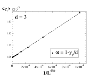
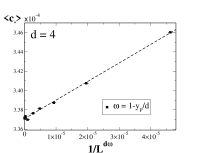
Figure 1: Plot of the approximate ground state cost per spin, $\left\langle c_{0}\right\rangle$, at bond-percolation $(p=p_{c})$ in dimension $d=3$ (top) and 4 (bottom) on lattices up to $L\leq 100.$ The data is plotted with respect to the presumed FSC, $1/L^{d\omega}$ with $\omega=1-y_{P}/d$, using $y_{P}=-1.29(1)$ in $d=3$ and $y_{P}=-1.574(6)$ in $d=4$, see Tab. 1. Data for $L<7$ (way off scale to be shown) deviates from the asymptotic scaling.

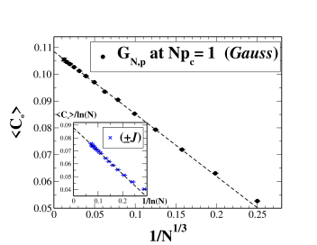
Figure 2: Plot of the average ground state cost $\left\langle C_{0}\right\rangle$ as a function of $1/N^{1/3},$ obtained with the reduction method described in Refs. [Boettcher, 2004a, b], for percolating random graphs $G_{N,p}$ (degree $Np=1)$ of sizes up to $N=2^{19}$, using a continuous (Gaussian) bond distribution. Apparently, the total cost itself is intensive and approached with $\left\langle C_{0}\right\rangle_{N}\sim\left\langle C_{0}\right\rangle_{\infty}+\frac{1}{2}\Upsilon/N^{1/3}$. Inset: Corresponding plot for discrete bonds, exhibiting entirely distinct scaling, $\left\langle C_{0}\right\rangle_{N}\sim\left\langle C_{0}\right\rangle_{\infty}\ln(N)+\Upsilon/2$.

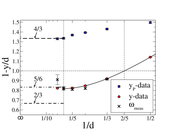
Figure 3: Plot of $1-y/d$ and the measured values, $\bar{\omega}$, in Tab. 1 as a function of inverse dimension $1/d$. The vertical lines marks the upper and lower critical dimensions of EA at $d_{u}=6$ (left) and $d_{l}\approx 5/2$ (right), at which $y=0$. Possible mean-field predictions to hold above $d_{u}$ are marked by horizontal lines: $\omega=4/3$ for lattices at $p=p_{c}$, $\omega=5/6$ for EA-lattices at $p>p_{c}$, and $\omega=2/3$ as predicted from simulations of SK. The extrapolations in Figs. 1 and 4 suggest the validity of Eq. (2) for all $d$, and it seems difficult to relate the FSC in SK to those of EA.

III Edwards-Anderson Model at the Percolation Threshold

As a demonstration of our approach, we first treat the problem on strongly diluted EA-lattices exactly at $p=p_{c}$, previously studied in Ref. [Boettcher and Marchetti, 2008]. The fractal lattice at $p_{c}$ is too ramified to sustain order and $y=y_{P}<0$ for all $d$.(Banavar et al., 1987) Polynomial-time algorithms have been used to achieve system sizes up to $N\approx 10^{8}$, i.e., $L\leq 11$ in $d=7$, and the results for $y_{P}$ are recounted in Tab. 1. With the available data, we focus on demonstrating its consistency with Eq. (2) by plotting it on the appropriate scale. The results for the extrapolation of the ground state cost for increasing system size $L$ according to Eq. (4) are shown in Fig. 1 for $d=3$ and 4. Indeed, the linearity of the plot on the scale $1/L^{d\omega}$ with $\omega=1-y_{P}/d$, as given in Tab. 1 for $p=p_{c}$, supports Eq. (2), as expected for $T_{c}=0$ and $y_{P}<0$.(Campbell et al., 2004) However, it is interesting to note that the data in Tab. 1 suggests $\omega\to 4/3$ for $d\to\infty$, as depicted in Fig. 3. In the large-$d$ limit, a lattice at $p=p_{c}\sim 1/(2d)$ is similar to an ordinary random graph(Bollobas, 1985) $G_{N,p}$ at percolation, $Np\to 1$, this would predict FSC of the form $1/N^{4/3}$ for the cost density of percolating $G_{N,p}$. As Fig. 2 shows, we do find an FSC with $\omega=4/3$ when using Gaussian bonds, except for the fact that the cost $\left\langle C_{0}\right\rangle$ itself in such a limit has become intensive. The energy remains trivially extensive, $E_{0}\sim-B\gg C_{0}$, as discussed above.

Fig. 2 also shows the corresponding result using a discrete ($\pm J_{0}$) bond distribution but the same graph ensemble. Note that the change in distribution affects an entirely different scaling. The leading-order difference can be explained by envisioning $G_{N,p}$ near percolation as a tree possessing $O\left(\ln N\right)$ weakly interlinked loops, each of length $O\left(\ln N\right)$, with half of those (1d-like) loops frustrated in a single bond: The total cost for discrete bonds of fixed weight $\left|J\right|=J_{0}$ is $\left\langle C_{0}\right\rangle_{N}\sim J_{0}\ln N$, while for continuous bonds this cost is mitigated by selecting the weakest weight, $\left|J\right|\sim J_{0}/\ln N$, in the loop and $\left\langle C_{0}\right\rangle_{N}$ approaches a constant value.

We conclude for $p=p_{c}$ that our results in finite $d$ connect well with those for $d\to\infty$, as long as we choose a continuous bond distribution in the mean-field limit. While non-universality is not unexpected when $T_{c}=0$,(Hartmann and Young, 2001) we will encounter it also for FSC when $T_{c}>0$ because FSC do not affect the thermodynamic limit.

IV Edwards-Anderson Model in the Glassy State

Parallel to the above case, we analyze our data for dilute EA-lattices in the glassy regime, $p>p_{c}$. However, this data had to be obtained in far more laborious simulations. While starting from lattices of comparable size, up to $N\sim 10^{8}$, the methods from Ref. [Boettcher and Marchetti, 2008] merely reduce each instance to a remainder of about $N_{R}\lesssim 10^{3}$ variables at the chosen values of $p>p_{c}$. (The choice of $p$ is crucial: larger values dramatically increase the remainder sizes, smaller values create long transients due to the proximity of $p_{c}$.) The cost $C_{0}$ of each remainder had to be optimized by local search with EO,(Boettcher and Percus, 2001) run with $O\left(N_{R}^{3}\right)$ updates.(Boettcher, 2004a) Depending on system size $L$ and dimension $d$, disorder averaging required $10^{4}-10^{7}$ instances to reduce statistical errors. In contrast to our earlier simulations,(Boettcher, 2004a, b) far more statistical accuracy for each energy average and new implementations to handle very large lattices efficiently are required here. While there is never a guarantee for finding actual ground states, we have applied similar safeguards to hold systematic errors below statistical errors as in previous investigations.(Boettcher and Percus, 2001; Boettcher, 2003; Hartmann and Rieger, 2004; Boettcher, 2010a) For instance, in $d=7$ at $L=11$ we have tested subsets of 100 instances at run-times of twice the normal setting and did not find a single deviation.

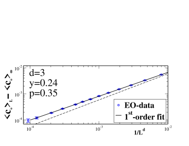
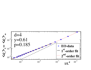
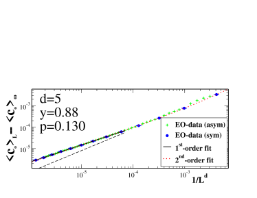
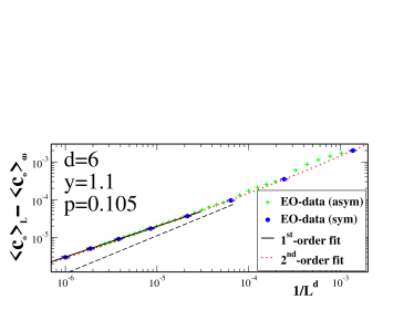
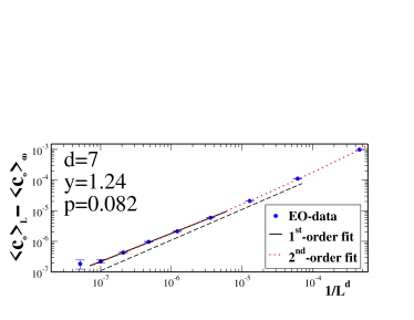
Figure 4: Double-logarithmic plots of the approximate ground state cost per spin, $\left\langle c_{0}\right\rangle_{L}=\left\langle C_{0}\right\rangle_{L}/L^{d}$, reduced by its numerically extrapolated limit value $\left\langle c_{0}\right\rangle_{\infty}=\lim_{L\to\infty}\left\langle c_{0}\right\rangle_{L}$, versus $1/L^{d}$ for dimensions $d=3,\ldots,7$. Subtracting off $\left\langle c_{0}\right\rangle_{\infty}$ highlights the FSC-term in Eq. (4). Simulated lattice sizes range from $L=3$ to $L\leq 25$ ($d=3$), $L\leq 20$ ($d=4$), $L\leq 15$ ($d=5$), and $L\leq 10$ ($d=6,7$) at respective bond densities $p=0.185$ ($d=4$), $p=0.13$ ($d=5$), $p=0.105$ ($d=6$), and $p=0.082$ ($d=7$). The $1^{\rm st}$-order fit (solid line) to obtain $\left\langle c_{0}\right\rangle_{\infty}$ and $\bar{\omega}$ using Eq. (4) only utilized the fitted data-points. The measured values for $\bar{\omega}$ are reported in Tab. 1. The $2^{\rm nd}$-order fit (dotted line), involving all data for $d=4,\ldots,7$, held previously fitted parameters fixed but added a further correction term to Eq. (4). This correction shows little effect on the asymptotic scaling, as solid and dotted lines virtually coincide. The dashed line for any “bulk” corrections of order $1/L^{d}$ is provided for reference only. Data (+) in $d=5,6$ obtained from asymmetric instances (labeled “asym”) was exclude from the fits; it is displayed to demonstrate its consistency, being systematically “arced” above the symmetric data.

To avoid the above-mentioned problem of wide separation between data points at $L$ and $L+1$ in higher $d$, we have also undertaken to simulate asymmetric instances of size $N=L^{d-m}(L+1)^{m}$ for $m=1,2,\ldots,d-1$. While we display that data as well, it proved unsuitable to fit. It merely serves to demonstrate that even such a minor variation in rather large, random instances resulted in sufficiently large systematic distortions from the $m=0$ data to be detectable with our heuristic.

The results of this effort for $d=3,\ldots,7$ are presented in Fig. 4. In each case, the raw data in the asymptotic scaling regime has been fit to the form in Eq. (4) to yield $\bar{\omega}=0.914(5)$ and $\left\langle c_{0}\right\rangle_{\infty}\approx 0.0425063$ with $\chi^{2}/ndf\approx 1.3$ ($d=3$), $\bar{\omega}=0.82(1)$ and $\left\langle c_{0}\right\rangle_{\infty}\approx 0.0063720$ with $\chi^{2}/ndf\approx 0.77$ ($d=4$), $\bar{\omega}=0.81(1)$ and $\left\langle c_{0}\right\rangle_{\infty}\approx 0.0022543$ with $\chi^{2}/ndf\approx 1.8$ ($d=5$), $\bar{\omega}=0.82(2)$ and $\left\langle c_{0}\right\rangle_{\infty}\approx 0.0014851$ with $\chi^{2}/ndf\approx 0.8$ ($d=6$), $\bar{\omega}=0.91(5)$ and $\left\langle c_{0}\right\rangle_{\infty}\approx 0.00061055$ ($d=7$). Each fitted value of $\bar{\omega}$ is close to $1-y/d$, see Tab. 1 and Fig. 3, except for $d=7$. For the largest $d$, the value of $\bar{\omega}$ trends higher, although it is difficult to judge whether asymptotic behavior has been reached. Fixing $\omega=1-y/d$ and using a $1/L^{d\omega}$-scale as in Fig. 1, a two-parameter linear fit (not shown) yields virtually identical values: $\left\langle c_{0}\right\rangle_{\infty}\approx 0.0063735$ ($d=4$), $\left\langle c_{0}\right\rangle_{\infty}\approx 0.0022546$ ($d=5$), $\left\langle c_{0}\right\rangle_{\infty}\approx 0.0014852$ ($d=6$), and $\left\langle c_{0}\right\rangle_{\infty}\approx 0.00061047$ ($d=7$). In Fig. 4 we have subtracted the fitetd value of $\left\langle c_{0}\right\rangle_{\infty}$ from each data point to be able to plot the remaining scaling form on a double-logarithmic plot, for better visibility.

To assess the effect of higher order corrections on our fits, we fixed the parameters of the $1^{\rm st}$-order fit and added another scaling correction term to Eq. (4) for a $2^{\rm nd}$-order fit, now including all points down to the smallest size, $L=3$. In each case, these corrections scaled with an exponent of $\approx 1.3-1.6$, about twice that of the leading correction. Shown as dotted lines in Fig. 4, these higher-order corrections have virtually no impact on the asymptotic behavior. We have tested that the existence of such a rapidly vanishing correction does not affect our results by more than 2% in $\bar{\omega}$.

V Conclusions

We conclude, first and foremost, that the ground-state FSC in EA are consistent with Eq. (2), for all $d\leq d_{u}=6$, whether $T_{c}=0$ ($p=p_{c}$) or $T_{c}>0$ ($p>p_{c}$). The connection with mean-field predictions is more complicated. The FSC exponent $\omega$ for EA does not approach its equivalent of $\omega_{SK}\approx 2/3$ in SK(Boettcher, 2005b; Aspelmeier et al., 2008; Boettcher, 2010b, 2003) at $d_{u}$, by far. As Fig. 3 shows, its mean-field limit seems more aligned with the result of $\omega\approx 0.8$ found for sparse-degree BL having a continuous bond distribution.(Boettcher, 2010a) There is no obvious reason why those BL would provide a more appropriate mean-field limit for EA, except for their sparse degree. In the computationally simpler case of EA at $p=p_{c}$, a similar approach for FSC to a sparse mean-field limit is even more apparent.

Beyond FSC, ground-state energy fluctuations provide another example where its exponent $\rho$ in EA does not reach the corresponding SK value for large $d$. It has been proven(Wehr and Aizenman, 1990) that those fluctuations are normal (i.e., $\rho=1/2$) for all $d$ in EA, whereas in SK it has a value of $\rho=5/6$.(Parisi and Rizzo, 2008) (In fact, it has been argued(Aspelmeier et al., 2003) that $\rho=1-y/d$ for $d>d_{u}$, for which Eq. (2) implies $\omega=\rho=5/6$ at $d_{u}$, consistent with our data in Tab. 1 and Fig. 3.) Again, BL with Gaussian bonds appear to have the right mean-field limit for EA, exhibiting $\rho=1/2$.(Boettcher, 2010b)

To sort out these behaviors we first note that both, $\omega$ and $\rho$, merely describe properties of the asymptotic approach to the thermodynamic limit and, hence, may exhibit non-universal (i.e., distribution-dependent) behavior, even though they can be related to other, universal exponents such as $y$. Non-universal, distribution-dependent behavior is far more prevalent for sparse mean-field spin glasses than for SK.(Boettcher, 2010a, b) For such properties, it ought not surprise that these sparse systems provide a better high-dimensional limit for EA than SK. After all, in studying EA we first take the limit $N=L^{d}\to\infty$ at fixed $d$ (for a sparse degree of $2d$) before we consider $d\to\infty$, whereas SK corresponds to the correlated limit, $N\to\infty$, $d\to\infty$ with degree $2d\sim N$ held fixed. In disordered systems, the order in which those limits are taken might well matter. However, the quest to understand the extend or possible break-down of RSB, which is known to describe the glassy state in sparse mean-field models(Mézard and Parisi, 2001; Mezard and Parisi, 2003) as well as SK, remains undiminished.

This work has been supported by grant DMR-0812204 from the National Science Foundation.

References

- Sherrington and Kirkpatrick (1975) D. Sherrington and S. Kirkpatrick, Phys. Rev. Lett. 35, 1792 (1975).
- Edwards and Anderson (1975) S. F. Edwards and P. W. Anderson, J. Phys. F 5, 965 (1975).
- Parisi (1979) G. Parisi, Phys. Rev. Lett. 43, 1754 (1979).
- Parisi (1980) G. Parisi, J. Phys. A 13, L115 (1980).
- Bray and Moore (1986) A. J. Bray and M. A. Moore, in Heidelberg Colloquium on Glassy Dynamics and Optimization, edited by L. Van Hemmen and I. Morgenstern (Springer, New York, 1986), p. 121.
- Fisher and Huse (1986) D. S. Fisher and D. A. Huse, Phys. Rev. Lett. 56, 1601 (1986).
- Franz et al. (1994) S. Franz, G. Parisi, and M. A. Virasoro, J. Phys. I (France) 4, 1657 (1994).
- Marinari et al. (1998) E. Marinari, G. Parisi, and J. J. Ruiz-Lorenzo, Phys. Rev. B 58, 14852 (1998).
- de Dominicis et al. (1998) C. de Dominicis, I. Kondor, and T. Temesári, in Spin Glasses and Random Fields, edited by A. Young (World Scientific, Singapore, 1998).
- Young (2008) A. P. Young, J. Phys. A: Math. Theor. 41, 324016 (2008).
- Krzakala et al. (2001) F. Krzakala, J. Houdayer, E. Marinari, O. C. Martin, and G. Parisi, Phys. Rev. Lett. 87, 197204 (2001).
- Katzgraber and Young (2003a) H. G. Katzgraber and A. P. Young, Phys. Rev. B 68, 224408 (2003a).
- Young and Katzgraber (2004) A. P. Young and H. G. Katzgraber, Phys. Rev. Lett. 93, 207203 (2004).
- Jörg et al. (2008) T. Jörg, H. G. Katzgraber, and F. Krza¸kała, Phys. Rev. Lett. 100, 197202 (2008).
- Wales (2003) D. J. Wales, Energy landscapes (Cambridge University Press, Cambridge, 2003).
- Katzgraber and Young (2003b) H. G. Katzgraber and A. P. Young, Phys. Rev. B 67, 134410 (2003b).
- Katzgraber and Young (2005) H. G. Katzgraber and A. P. Young, Phys. Rev. B 72, 184416 (2005).
- Leuzzi et al. (2008) L. Leuzzi, G. Parisi, F. Ricci-Tersenghi, and J. J. Ruiz-Lorenzo, Phys. Rev. Lett. 101, 107203 (pages 4) (2008).
- Boettcher (2004a) S. Boettcher, Euro. Phys. J. B 38, 83 (2004a).
- Boettcher (2004b) S. Boettcher, Europhys. Lett. 67, 453 (2004b).
- Boettcher (2005a) S. Boettcher, Phys. Rev. Lett. 95, 197205 (2005a).