General analysis of decay chains with three-body decays involving missing energy
Chien-Yi Chen1, A. Freitas2
1 Department of Physics, Carnegie Mellon University, Pittsburgh, PA
15213, USA
2
Pittsburgh Particle-physics Astro-physics & Cosmology Center
(Pitt-PACC),
Department of Physics & Astronomy, University of Pittsburgh,
Pittsburgh, PA 15260, USA
Abstract
A model-independent analysis of decays of the form () is presented, including the possibility that this three-body decay is preceded by an additional decay step . Here , and are heavy new-physics particles and stands for a quark jet. It is assumed that escapes direct detection in a collider experiment, so that one cannot kinematically reconstruct the momenta of the new particles. Instead, information about their properties can be obtained from invariant-mass distributions of the visible decay products, the di-lepton () and jet-lepton () invariant-mass distributions. All possible spin configurations and renormalizable couplings of the new particles are considered, and explicit expressions for the invariant-mass distributions are derived, in a formulation that separates the coupling parameters from the spin and kinematic information. In a numerical analysis, it is shown how these properties can be determined independently from a fit to the and distributions.
1 Introduction
A large range of models have been proposed that predict new particles within the reach of the Large Hadron Collider (LHC). Since there is currently very little evidence for favoring one model over the others, it will be essential to analyze a potential new-physics signal in the LHC data in a model-independent approach, by independently determining the properties of each of the produced particles. Recently, this idea has gained increased interest, and several groups have worked on constructing such model-independent setups for a number of different observable signatures, see Refs. [4, 3, 1, 2]. A particularly challenging scenario are processes that result in the production of new weakly interacting massive particles (WIMPs), which are invisible to the detector. WIMPs are predicted in many models as hypothetical dark matter candidates. In these models, the stability of the WIMP is a consequence of some (discrete) symmetry, under which it is charged. As a result, it can be produced only in pairs at colliders, leading to challenging events with at least two invisible objects. At hadron colliders like the LHC there are not enough kinematical constraints in events of this type for the direct reconstruction of the momenta of all particles involved.
One approach to this problem is motivated by the fact that models predict additional new particles, which can decay into the stable WIMP. In this case, one can have cascade decay chains, which go through multiple decay steps before ending with the stable WIMP, so that one can construct invariant-mass distributions of the visible decay products of this cascade. The kinematic endpoints of these distributions yield information about the masses [5] of the new heavy particles, while the shape is sensitive to their spins [6, 1, 7, 2]. Refs. [1, 2] have analyzed decay chains built up from a sequence of two-body decays in a model-independent way, by considering arbitrary spin assignments [1] and also using general parametrizations for the coupling for the new particles [2].
However, for scenarios with relatively small splittings in the mass spectrum of the new-physics particles, it can often happen that the last decay step is a three-body decay mediated by a heavier off-shell particle, see right-hand side of Fig. 1. In Ref. [8], three-body decays have been analyzed in order to distinguish gluinos, the supersymmetric partners of gluons, from a Kaluza-Klein (KK) gluons in universal extra dimensions (UED). A model-independent study of three-body decays has been presented in Ref. [9], but only in the limit of an asymptotically large mass of the intermediate off-shell particles. In typical supersymmetry and UED scenarios, however, this limit is often not a good approximation.
In this work, three-body decays of the form will be analyzed in a model-independent setup without assumptions about the values of the masses of the new-physics particles. Here is a massive new particle that decays into the WIMP and two SM leptons through the off-shell exchange of a third new particle or the SM -boson, see Fig. 1***In general, besides the -boson, a bosonic new-physics particle ( a or a Higgs boson) may also appear in the decay topology II. However, the branching of such a particle into leptons is strongly constrained by data on four-fermion contact interactions [10], and thus its contribution will be neglected here.. The spins of , , and , their coupling parameters, and the mass of the particle will be kept as free quantities that have to be extracted from the experimental data. We only impose the constraint , or , to ensure that we have an actual three-body decay. Without these constraints the three-body decay would decompose into two two-body decays, which is a scenario that has been discussed in detail in the literature cited above.
Furthermore, we also consider the case that this three-body decay is the second step of a cascade decay of the form , where refers to a SM quark (antiquark), see Fig. 1. Such a decay chain would lead to two independent observable invariant-mass distributions, a di-lepton () invariant-mass distribution, and a jet-lepton () invariant-mass distribution, where the jet emerges from the fragmentation of the quark or antiquark.
For both of these cases, we investigate the simultaneous determination of the spins and couplings of the new particles , , and from the shapes of these distributions. The determination of the masses from kinematic endpoints has been discussed elsewhere [5], and here we will simply assume that the masses of the particles , and are already known. On the other hand, the mass of the off-shell intermediate particle can not be extracted from the kinematic endpoints, and we will study if instead it can be constrained from the shapes of the distributions.
Our analysis closely follows the conventions of Ref. [2]. After introducing the relevant spin and coupling representations in section 2, the calculation of the and invariant-mass distributions is described in section 3. In section 4 we present a procedure for determining the spins and couplings of the new particles, as well as the mass of the intermediate particle , by fitting the theoretically calculated functions to the experimentally observed distributions. The method is illustrated by applying it in two numerical examples. Finally, our main conclusions are summarized in section 5.
2 Setup
The three-body decay of a heavy new particle into two opposite-sign same-flavor leptons and a second new particle ,
| (1) |
is mediated either by an off-shell heavy new particle (with ) or a SM -boson (with ). We also consider the possibility that eq. (1) occurs as the last step of a longer decay chain,
| (2) | ||||
Here is a QCD triplet, while and are electrically charged and neutral QCD singlets, respectively. For the purpose of this work, it is assumed that and are self-conjugate ( they are their own antiparticles)†††Some new physics models predict decay chains with non-self-conjugate neutral heavy particles, which lead to distinct phenomenological features [11], but this case will not be considered here.. Furthermore, it is assumed that , , , and are charged under some symmetry which ensures that is stable and escapes from the detector without leaving a signal.
In general, it is difficult to experimentally determine the overall strength of the couplings in the decay chain since the width of weakly decaying particles is typically small compared to the experimental resolution. Consequently, only the shape of the observable invariant-mass distributions will be considered here, similar to earlier studies on spin determination [6, 1, 2, 8, 9]. All expressions for these distributions presented in the following sections therefore include an arbitrary, but constant, normalization factor.
Example 1 S F S F 2 F S F S 3 F S F V F V F S 5 F V F V 6 S F V F 7 F S S 8 F S V F V S 10 F V V 11 S F F
Table 1 lists all possible spin assignments for the particles in any renormalizable theory with fields of spin 0 (scalars), spin 1/2 (fermions) and/or spin 1 (vector bosons). Also shown are examples for realizations of these assignments in known models.
The chirality of the fermion couplings depend on the details of the new physics and thus are a priori unknown. Following Ref. [2], we introduce arbitrary left- and right-handed components. For scalar-fermion-fermion vertices, the interaction Lagrangians are defined as
| (3) | |||
| (4) | |||
| (5) | |||
| (6) | |||
| (7) | |||
| (8) |
where . For vector-fermion-fermion couplings, must be replaced by in (3), etc. After normalizing the overall coupling strength to unity, each vertex can be parametrized by a single angle , , or ,
| (9) | ||||||||
As will be shown later, the entire parameter space for the couplings can be covered by restricting the angles to the intervals .
The form of the vertices is uniquely determined by Lorentz symmetry and CP properties (since the -boson is CP-odd, while the self-conjugate and are C-even):
| (10) | |||
| (11) | |||
| (12) | |||
| (13) | |||
| (14) |
where again the coupling constants have been normalized to unity.
In an experimental analysis, it is impossible to tell on an event-by-event basis whether a quark or an antiquark is emitted in the first stage of eq. (2), whether the cascade decay was initiated by a particle or its antiparticle . However, the observable invariant-mass distribution may depend significantly on the fraction of events stemming from decays versus the fraction of events stemming from decays, with .
As pointed out in Ref. [2], the ratio of and is very difficult to determine without model assumption and thus should be treated as a free parameter. The distribution depends on and only through the combinations and . It is therefore convenient to introduce the parameter , defined by [2]
| (15) | ||||
| (16) |
From the analysis of the invariant-mass distribution one can only obtain a constraint on , but not on and independently.
3 Invariant-mass distributions
As pointed out above, it is difficult to discriminate experimentally between the decay chain in Fig. 1, with a quark emitted in the first stage, and its charge-conjugated version with an antiquark emitted in the first stage, since both quark and antiquark fragment into jets. Therefore the only relevant observable invariant-mass distributions are the (lepton-lepton) distribution and the (jet-lepton) distribution.
There is no distinction between the two leptons in the three-body decay, in contrast to the situation when can be produced on-shell ( for ) in which case one can define a “near” and a “far” lepton [5, 6, 1, 7, 2].
Explicit expressions for the and distributions are obtained by computing the squared matrix elements for the different spin configurations =1–11 in Tab. 1 and integrating over the remaining phase space variables. A convenient choice for the phase space integration is given by
| (17) | ||||
| (18) | ||||
where . In these equations, denote the matrix elements for the 3-body or (3+1)-body decay processes, respectively, while is the invariant mass of particle and one of the leptons, and is the angle between the plane spanned by the lepton-lepton system and the quark in the reference frame of . The charge of the lepton in and has been specified for definiteness, but one can equally well choose the variables and . and are unspecified normalization constants.
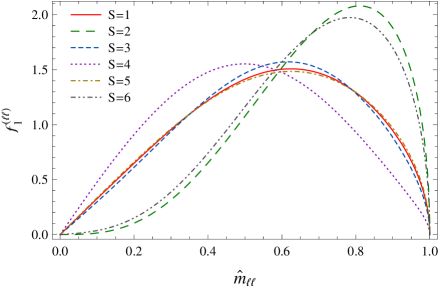
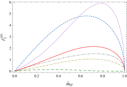
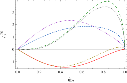
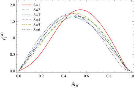
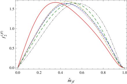
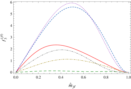
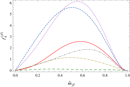
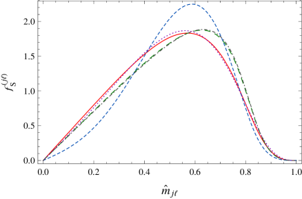
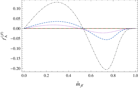
As mentioned above, the endpoints of the invariant-mass distributions can be used to obtain information about the masses , and of the particles that are produced on-shell in the cascade, while the shapes of the distributions depend on the couplings and spins of the particles –. Focusing on the latter, it is convenient to define the distributions and in terms of unit-normalized invariant masses
| (19) | ||||||
| (20) |
For the spin configurations =1–6, the dependence on the coupling parameters can be cast into the form
| (21) | ||||
| (22) |
where the functions and are independent of the coupling parameters, but they contain the entire kinematical and spin information, including the dependence on the particle masses. Note that and receive contributions only from the interference term between the - and -channel diagrams in the upper part of Fig. 1, see also Ref. [8].
From eqs. (21),(22) one can see that without loss of generality the coupling parameters can be restricted to the intervals , as already mentioned in the previous section.
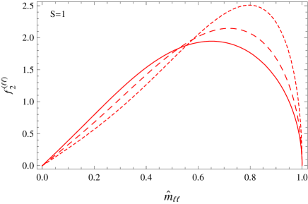
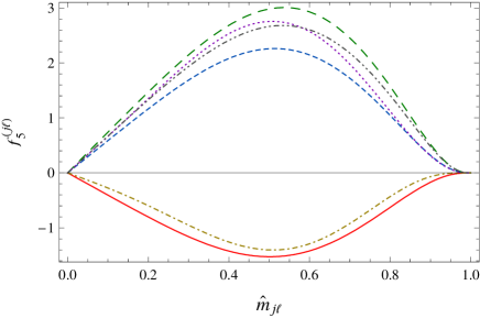
For =7–11, the coupling is uniquely fixed up to an overall coupling constant, so that there is only one term for the lepton-lepton invariant-mass distribution. However, there are two possible terms for the jet-lepton invariant-mass distribution:
| (23) | ||||
| (24) |
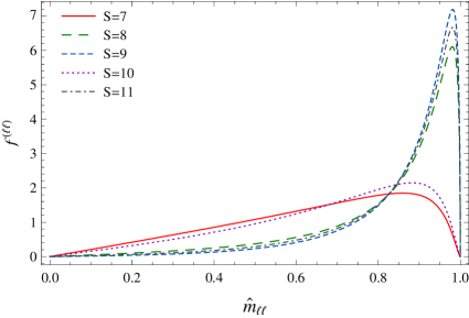
The lepton-lepton distribution can be expressed in terms of compact analytical formulae. On the other hand, the analytical results for are very lengthy, so that instead we chose to perform the last integration step (over ) numerically.
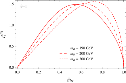
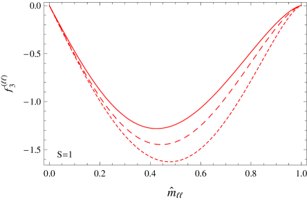
Explicit expressions for the functions are available for free download (see appendix). Figs. 2–4 depict the distribution functions for a sample mass spectrum. In the figures, the overall normalization constants have been fixed by requiring that , , , and are unit-normalized. The right column of Fig. 2 also illustrates how the distributions vary with the mass of the off-shell intermediate particle , for the example of the spin configuration =1.
 |
 |
 |
 |
 |
 |
 |
 |
 |
 |
 |
4 Analysis method
In this section we will discuss the determination of the spins and couplings parameters of the new particles, as well as the mass of the off-shell particle , by fitting the theoretically calculated distributions to experimental data. The general procedure will be outlined in the next subsection, while its application will be demonstrated in subsection 4.2 for two concrete numerical examples.
4.1 Conceptual procedure
The analysis is based on a binned fit for the and distributions. In this fit, the binned histogram for the data is compared with theoretical histograms obtained by numerically integrating the functions and , defined in the previous section, over the interval covered by each bin. In the fit, the coupling parameters and the mass are kept as free parameters. Varying over these parameters and the spin configuration , the best-fit result is found as the set of numbers that minimizes the value.
During the fit procedure, for every given choice of the parameters , the theoretical histograms for the and distributions are normalized such that the total number of events in the theoretical histogram agrees with the number of events in the data histogram. In practice, this normalization is most easily carried out numerically.
In general, it may happen that there is not a unique solution for the minimum value, but instead several degenerate best-fit points are obtained. In such a situation, the coupling parameters and/or the spin assignment cannot be determined uniquely from the observable distributions of the decays (1),(2) alone.
4.2 Numerical examples
To illustrate the fitting procedure, its application is demonstrated by performing a fit to mock-up data histograms. This section is based on the parton-level description of the decay processes (1),(2) as described in the previous sections, thus neglecting issues such as backgrounds, jet combinatorics and energy smearing, which are relevant in a realistic experimental setup. However, earlier studies [5, 14] have shown that, for mass parameters similar to the ones chosen here, it is possible to obtain a clean, almost background-free sample of signal events with relatively simple selection cuts.
Let us consider two sample choices for the hypothetical data:
-
“Data” A:
GeV, GeV, GeV, GeV
(corresponding to the MSSM decay chain ); -
“Data” B:
GeV, GeV, GeV
(corresponding to the MSSM decay chain ).
For each case, we have computed “data” histograms with 10 bins each for the and the distributions, corresponding to a total of 1000 events. Then we have performed a fit of the theoretical distribution functions to these fake “data” histogram for each of the spin configurations =1–11, searching for the minimum value as a function of the parameters , and ‡‡‡For the spin configurations =7–11, the non-zero -boson width has been included although its numerical impact is not very important for the masses chosen here..
a) “Data” A, using only distribution:
| best-fit parameters | ||||
|---|---|---|---|---|
| [GeV] | ||||
| 1 [SFSF] | 0.00 | 0.00 | 1.57 | 200.0 |
| 2 [FSFS] | 0.00 | 1.22 | 1.05 | 209 |
| 3 [FSFV] | 0.00 | 1.14 | 0.43 | 197.7 |
| 4 [FVFS] | 0.27 | 1.34 | 0.23 | 216 |
| 5 [FVFV] | 0.05 | 0.38 | 0.38 | 197 |
| 6 [SFVF] | 0.05 | 0.65 | 0.92 | 191.3 |
| 7 [FSS] | 140 |
|---|---|
| 8 [FSV] | 3100 |
| 9 [FVS] | 4200 |
| 10 [FVV] | 290 |
| 11 [SFF] | 3700 |
b) “Data” A, using both and distributions:
| best-fit parameters | |||||
|---|---|---|---|---|---|
| [GeV] | |||||
| 1 [SFSF] | 0 | 0.00 | 1.57 | 0.00 | 200.0 |
| 2 [FSFS] | 150 | 0.08 | 0.07 | 1.57 | 754 |
| 3 [FSFV] | 87 | 1.57 | 1.57 | 0.29 | 210 |
| 4 [FVFS] | 48 | 1.19 | 0.00 | 1.57 | 220 |
| 5 [FVFV] | 46 | 0.93 | 0.25 | 1.57 | 224 |
| 6 [SFVF] | 37 | 0.50 | 0.53 | 1.57 | 197.4 |
| best-fit | ||
|---|---|---|
| 7 [FSS] | 200 | ? |
| 8 [FSV] | 3100 | ? |
| 9 [FVS] | 4300 | 0.39 |
| 10 [FVV] | 330 | 1.57 |
| 11 [SFF] | 3700 | 1.08 |
a) “Data” B, using only distribution:
| best-fit parameters | ||||
| [GeV] | ||||
| 1 [SFSF] | 1200 | 0.79 | 0.79 | |
| 2 [FSFS] | 670 | ? | ? | |
| 3 [FSFV] | 2200 | ? | ? | |
| 4 [FVFS] | 1100 | ? | ? | |
| 5 [FVFV] | 720 | |||
| 6 [SFVF] | 740 | 1.57 | 0.00 | |
| 7 [FSS] | 1600 |
|---|---|
| 8 [FSV] | 16 |
| 9 [FVS] | 8.7 |
| 10 [FVV] | 1100 |
| 11 [SFF] | 0.00 |
b) “Data” B, using both and distributions:
| best-fit parameters | |||||
|---|---|---|---|---|---|
| [GeV] | |||||
| 1 [SFSF] | 1200 | 0.78 | 0.77 | 0.00 | |
| 2 [FSFS] | 690 | ? | ? | ? | |
| 3 [FSFV] | 2300 | ? | ? | ? | |
| 4 [FVFS] | 1100 | 1.25 | 0.43 | 1.32 | |
| 5 [FVFV] | 750 | 0.46 | 0.46 | 1.57 | |
| 6 [SFVF] | 760 | 1.57 | 0.00 | ? | |
| best-fit | ||
|---|---|---|
| 7 [FSS] | 1600 | ? |
| 8 [FSV] | 25 | ? |
| 9 [FVS] | 59 | 0.00 |
| 10 [FVV] | 1100 | 0.00 |
| 11 [SFF] | 0.00 | 0.00 |
The results are shown in Tables 2 and 3. From Tab. 2 one can see that when only information about the distribution is available, it is difficult to distinguish the “data” A (based on the spin configuration =1) from the spin configurations =2–6. The underlying reason is that for each of these spin configurations there are three unknown continuous parameters, , and , which can be adjusted so as to mimic the data distribution.
On the other hand, the spin configurations =7–11 can be distinguished from “data” A with high significance, using only the distribution. This is a consequence of the fact that there are no free parameters to adjust in for =7–11, and that these spin configurations correspond to a different diagram topology (Topology II in Fig. 1 instead of topology I).
If both the and distributions are included in the fit, all possible spin configurations can be discriminated with at least six standard deviations, for the given number of 1000 events.
For the second example, it is evident from Tab. 3 that “data” B can be distinguished from all other spin configurations =1–10 by just using the distribution. In fact, for all combinations except =8 and =9 the significance for this discrimination is very high and is not improved substantially by including the distribution in the fit. Also note that the best-fit results for =1–6 are obtained for very large values of , since increasing values of shift the distribution toward larger values of , see Fig. 2 (right), leading to better agreement with the reference case =11, see Fig 4.
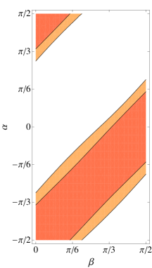
In addition to the spin determination, the couplings of the new particles and the mass of the off-shell particle can in principle be extracted from the fit to the invariant-mass distributions. This is shown in Fig. 5 for the example of “data” A. The panels (a) and (b) in the figure depict the constraints on , and obtained from fitting the distribution alone, assuming that =1 is the correct spin configuration. If a fit to both the and distributions is performed, one obtains the results in panels (c) and (d). As evident from the plots, the inclusion of the distribution does not only lead to a constraint on (which cannot be obtained from ), but also to improved bounds on and .
5 Summary
In this paper, a general analysis of three-body decays of the form , leading to a pair of opposite-sign leptons and one invisible particle , has been presented. This decay process can occur in many proposed new-physics models, either from direct production of the particle at the LHC, or from a cascade decay of the type , both of which have been studied here.
No assumptions about the masses, spins and couplings of the participating new-physics particles have been made, including the off-shell particle mediating the three-body decay. Instead, all possible spin configurations and coupling form factors have been considered. Experimentally, the masses, spins and coupling parameters may be determined from measuring the invariant-mass distributions of the visible decay products.
In the present case, there are two independent distributions, one with respect to the di-lepton () invariant mass, and the other with respect to the jet-lepton () invariant mass. Results for both have been obtained in terms of relatively compact analytical functions or one-dimensional integral representations.
In two concrete numerical examples, it has been tested how well the properties of the new-physics particles , , and can be determined from these two invariant-mass distributions. It turns out that the di-lepton invariant-mass distributions alone is sometimes not sufficient to uniquely determine the spins and coupling parameters. However, if the longer two-step cascade decay chain is observed, and one can measure both the and invariant-mass distributions, it is possible to unambiguously discriminate between all possible spin configuration with high significance. Furthermore, one can independently constrain all coupling parameters and the mass of the off-shell mediator , up to an intrinsic two-fold ambiguity.
The results presented here are based on a parton-level analysis. In a realistic experimental environment, the significance for the model discrimination and the precision for the parameter determination may be diluted by jet energy smearing and combinatorics, but the essential features and main conclusions are not affected substantially by these effects.
Acknowledgements
C.-Y. C. acknowledges support by The George E. and Majorie S. Pake Fellowship during part of this project. Also, he is grateful for the hospitality of the Theoretical Advanced Studies Institute (TASI 2011) at the University of Colorado at Boulder, where part of this work was done. The research of A. F. is supported partially by the National Science Foundation under grant PHY-0854782.
Appendix: Formulae for invariant-mass distributions
Explicit expressions for the functions and are avaiable in Mathematica format at http://www.pitt.edu/~afreitas/dec3.tgz. Note that the expressions in this file are not normalized, since in practice the normalization is best carried out numerically as described in section 4.1. The results for are given as analytical formulae, while are presented in terms of one-dimensional integral representations of the form
| (25) |
References
-
[1]
C. Athanasiou, C. G. Lester, J. M. Smillie, B. R. Webber,
JHEP 0608, 055 (2006);
J. M. Smillie, Eur. Phys. J. C51, 933-943 (2007). - [2] M. Burns, K. Kong, K. T. Matchev, M. Park, JHEP 0810, 081 (2008).
- [3] C.-Y. Chen, A. Freitas, JHEP 1102, 002 (2011).
-
[4]
T. Han, I. Lewis, Z. Liu,
JHEP 1012, 085 (2010);
J. Andrea, B. Fuks, F. Maltoni, arXiv:1106.6199 [hep-ph];
J. Kumar, A. Rajaraman, B. Thomas, arXiv:1108.3333 [hep-ph];
B. Grinstein, A. L. Kagan, M. Trott, J. Zupan, arXiv:1108.4027 [hep-ph]. -
[5]
I. Hinchliffe, F. E. Paige, M. D. Shapiro, J. Soderqvist, W. Yao,
Phys. Rev. D55, 5520-5540 (1997);
B. C. Allanach, C. G. Lester, M. A. Parker, B. R. Webber, JHEP 0009, 004 (2000);
K. Kawagoe, M. M. Nojiri, G. Polesello, Phys. Rev. D71, 035008 (2005);
B. K. Gjelsten, D. J. Miller, P. Osland, JHEP 0412, 003 (2004);
B. K. Gjelsten, D. J. Miller, P. Osland, JHEP 0506, 015 (2005). -
[6]
A. J. Barr,
Phys. Lett. B596, 205-212 (2004);
J. M. Smillie, B. R. Webber, JHEP 0510, 069 (2005);
A. Alves, O. Eboli, T. Plehn, Phys. Rev. D74, 095010 (2006);
L.-T. Wang, I. Yavin, JHEP 0704, 032 (2007);
C. Kilic, L.-T. Wang, I. Yavin, JHEP 0705, 052 (2007);
W. Ehrenfeld, A. Freitas, A. Landwehr, D. Wyler, JHEP 0907, 056 (2009). - [7] D. J. Miller, P. Osland, A. R. Raklev, JHEP 0603, 034 (2006).
- [8] C. Csaki, J. Heinonen, M. Perelstein, JHEP 0710, 107 (2007).
- [9] L. Edelhäuser, W. Porod, R. K. Singh, JHEP 1008, 053 (2010).
- [10] J. Alcaraz et al. [ALEPH and DELPHI and L3 and OPAL and LEP Electroweak Working Group Collaborations], hep-ex/0612034.
-
[11]
S. Y. Choi, M. Drees, A. Freitas, P. M. Zerwas,
Phys. Rev. D78, 095007 (2008);
S. Y. Choi, D. Choudhury, A. Freitas, J. Kalinowski, J. M. Kim, P. M. Zerwas, JHEP 1008, 025 (2010). - [12] S. P. Martin, in “Perspectives on supersymmetry II,” ed. G. L. Kane, World Scientifc, Singapore (2010), pp. 1–153 [hep-ph/9709356].
-
[13]
T. Appelquist, H. C. Cheng, B. A. Dobrescu,
Phys. Rev. D 64, 035002 (2001);
B. A. Dobrescu, E. Pontón, JHEP 0403, 071 (2004);
G. Burdman, B. A. Dobrescu, E. Pontón, JHEP 0602, 033 (2006). - [14] B. K. Gjelsten et al., in G. Weiglein et al. [LHC/LC Study Group Collaboration], Phys. Rept. 426, 47-358 (2006).