Ranked Sparse Signal Support Detection

Abstract

This paper considers the problem of detecting the support (sparsity pattern) of a sparse vector from random noisy measurements. Conditional power of a component of the sparse vector is defined as the energy conditioned on the component being nonzero. Analysis of a simplified version of orthogonal matching pursuit (OMP) called sequential OMP (SequOMP) demonstrates the importance of knowledge of the rankings of conditional powers. When the simple SequOMP algorithm is applied to components in nonincreasing order of conditional power, the detrimental effect of dynamic range on thresholding performance is eliminated. Furthermore, under the most favorable conditional powers, the performance of SequOMP approaches maximum likelihood performance at high signal-to-noise ratio.

I Introduction

Sets of signals that are sparse or approximately sparse with respect to some basis are ubiquitous because signal modeling often has the implicit goal of finding such bases. Using a sparsifying basis, a simple abstraction that applies in many settings is for

$$\mathbf{y}\ =\ \mathbf{A}\mathbf{x}+\mathbf{d}$$ (1)

to be observed, where $\mathbf{A}\in{\mathbb{R}}^{m\times n}$ is known, $\mathbf{x}\in{\mathbb{R}}^{n}$ is the unknown sparse signal of interest, and $\mathbf{d}\in{\mathbb{R}}^{m}$ is random noise. When $m<n$, constraints or prior information about $\mathbf{x}$ are essential to both estimation (finding vector $\widehat{\mathbf{x}}(\mathbf{y})$ such that $\|\mathbf{x}-\widehat{\mathbf{x}}\|$ is small) and detection (finding index set $\hat{I}(\mathbf{y})$ equal to the support of $\mathbf{x}$). The focus of this paper is on the use of magnitude rank information on $\mathbf{x}$—in addition to sparsity—in the support detection problem. We show that certain scaling laws relating the problem dimensions and the noise level are changed dramatically by exploiting the rank information in a simple sequential detection algorithm.

The simplicity of the observation model (1) belies the variety of questions that can be posed and the difficulty of precise analysis. In general, the performance of any algorithm is a complicated function of $\mathbf{A}$, $\mathbf{x}$, and the distribution of $\mathbf{d}$. To enable results that show the qualitative behavior in terms of problem dimensions and a few other parameters, we assume the entries of $\mathbf{A}$ are i.i.d. normal and describe $\mathbf{x}$ by its energy and its smallest-magnitude nonzero entry.

We consider a partially-random signal model

$$x_{j}\ =\ b_{j}\,s_{j},\qquad j=1,\,2,\,\ldots,\,n,$$ (2)

where components of vector $\mathbf{b}$ are i.i.d. Bernoulli random variables with $\Pr(b_{j}=1)=1-\Pr(b_{j}=0)=\lambda>0$ and $\mathbf{s}$ is a nonrandom parameter vector with all nonzero entries. The value $s_{j}^{2}$ represent the conditional power of the component $x_{j}$ in the event that $b_{j}=1$. We consider the problem where the estimator knows neither $b_{j}$ nor $s_{j}$, but may know the order or rank of the conditional powers. In this case, the estimator can, for example, sort the components of $\mathbf{s}$ in an order such that

$$|s_{1}|\ \geq\ |s_{2}|\ \geq\ \cdots\ \geq\ |s_{n}|\ >\ 0.$$ (3)

The main contribution of this paper is to show that this rank information is extremely valuable. A stylized application in which the conditional ranks can be known is random access communication as described in [1]. Irrespective of this application, we show that when conditional rank information is available, a very simple detector, termed sequential orthogonal matching pursuit (SequOMP), can be effective. The SequOMP algorithm is a one-pass version of the well-known orthogonal matching pursuit (OMP) algorithm (see references below). Similar to several works in sparsity pattern recovery [2, 3, 4], we analyze the performance of SequOMP by estimating a scaling on the minimum number of measurements $m$ to asymptotically reliably detect the sparsity pattern (support) of $\mathbf{x}$ in the limit of large random matrices $\mathbf{A}$. Although the SequOMP algorithm is extremely simple, we show:

• When the power orders are known and the signal-to-noise ratio (SNR) is high, the SequOMP algorithm exhibits a scaling in the minimum number of measurements for sparsity pattern recovery that is within a constant factor of the more sophisticated lasso and OMP algorithms. In particular, SequOMP exhibits a resistance to large dynamic ranges, which is one of the main motivations for using lasso and OMP.

• When the power profile can be optimized, SequOMP can achieve measurement scaling for sparsity pattern recovery that is within a constant factor of optimal ML detection. This scaling is better than the best known sufficient conditions for lasso and OMP.

The results are not meant to suggest that SequOMP is a good algorithm in any sense: other algorithms such as OMP can perform dramatically better. The point is to concretely and provably demonstrate the value of conditional rank information.

I-A Related Work

Under an i.i.d. Gaussian assumption on $\mathbf{d}$, maximum likelihood estimation of $\mathbf{x}$ under a sparsity constraint is equivalent to finding sparse $\widehat{\mathbf{x}}$ such that $\|\mathbf{y}-\mathbf{A}\widehat{\mathbf{x}}\|_{2}$ is minimized. This is called optimal sparse approximation of $\mathbf{y}$ using dictionary $\mathbf{A}$, and it is NP-hard [5]. Several greedy heuristics (matching pursuit [6] and its variants with orthogonalization [7, 8, 9] and iterative refinement [10, 11]) and convex relaxations (basis pursuit [12], lasso [13], Dantzig selector [14], and others) have been developed for sparse approximation, and under certain conditions on $\mathbf{A}$ and $\mathbf{y}$ they give optimal or near-optimal performance [15, 16, 17]. Results showing that near-optimal estimation of $\mathbf{x}$ is obtained with convex relaxations, pointwise over compressible $\mathbf{x}$ and with high probability over some random ensemble for $\mathbf{A}$, form the heart of the compressed sensing literature [18, 19, 20]. Under a probabilistic model for $\mathbf{x}$ and certain additional assumptions, exact asymptotic performances of several estimators are known [21].

Our interest is in recovery or detection of the support (or sparsity pattern) of $\mathbf{x}$ rather than the estimation of $\mathbf{x}$. In the noiseless case of $\mathbf{d}=0$, optimal estimation of $\mathbf{x}$ can yield $\widehat{\mathbf{x}}=\mathbf{x}$ under certain conditions on $\mathbf{A}$; estimation and detection then coincide, and some papers cited above and notably [22] contain relevant results. In the general noisy case, direct analysis of the detection problem has yielded much sharper results.

A standard formulation is to treat $\mathbf{s}$ as a nonrandom parameter vector and $\mathbf{b}$ as either nonrandom with weight $k$ or random with a uniform distribution over the weight-$k$ vectors. The minimum probability of detection error is then attained with maximum likelihood (ML) detection. Sufficient conditions for the success of ML detection are due to Wainwright [2]; necessary conditions based on channel capacity were given by several authors [23, 24, 25, 26], and conditions more stringent in many regimes and a comparison of results appears in [4]. Necessary and sufficient conditions for lasso were determined by Wainwright [3]. Sufficient conditions for orthogonal matching pursuit (OMP) were given by Tropp and Gilbert [27] and improved by Fletcher and Rangan [28]. Even simpler than OMP is a thresholding algorithm analyzed in a noiseless setting in [29] and with noise in [4]. These results are summarized in Table I, using terminology defined formally in Section II.

I-B Paper Organization

The remainder of the paper is organized as follows. The setting is formalized in Section II. In particular, we define all the key problem parameters. Common algorithms and previous results on their performances are then presented in Section III. We will see that there is a potentially-large performance gap between the simplest thresholding algorithm and the optimal ML detection, depending on the signal-to-noise ratio (SNR) and the dynamic range of $\mathbf{x}$. Section IV presents a new detection algorithm, sequential orthogonal matching pursuit (SequOMP), that exploits knowledge of conditional ranks. Numerical experiments are reported in Section V. Conclusions are given in Section VI, and proofs are relegated to the Appendix.

II Problem Formulation

In the observation model $\mathbf{y}=\mathbf{A}\mathbf{x}+\mathbf{d}$, let $\mathbf{A}\in{\mathbb{R}}^{m\times n}$ and $\mathbf{d}\in{\mathbb{R}}^{n}$ have i.i.d. $\mathcal{N}(0,1/m)$ entries. This is a normalization under which the ratio of conditional total signal energy to total noise energy

$$\mbox{\small SNR}(\mathbf{x})\ =\ \frac{\mathbf{E}[\|\mathbf{A}\mathbf{x}\|^{2}\mid\mathbf{x}]}{\mathbf{E}[\|\mathbf{d}\|^{2}]}$$ (4)

simplifies to

$$\mbox{\small SNR}(\mathbf{x})\ =\ \|\mathbf{x}\|^{2}.$$ (5)

Let

$$I_{\rm true}\ =\ \left\{~{}j\in\{1,2,\ldots,n\}~{}:~{}x_{j}\neq 0~{}\right\}$$

denote the support of $\mathbf{x}$. Using signal model (2),

$$I_{\rm true}\ =\ \left\{~{}j\in\{1,2,\ldots,n\}~{}:~{}b_{j}=1~{}\right\}.$$

The sparsity level of $\mathbf{x}$ is $k=|I_{\rm true}|$.

An estimator produces an estimate $\hat{I}=\hat{I}(\mathbf{y})$ of $I_{\rm true}$ based on the observed noisy vector $\mathbf{y}$. Given an estimator, its probability of error

$$p_{\rm err}\ =\ \Pr\left(\hat{I}\neq I_{\rm true}\right)$$ (6)

is taken with respect to randomness in $\mathbf{A}$, noise vector $\mathbf{d}$, and signal $\mathbf{x}$. Our interest is in relating the scaling of problem parameters with the success of various algorithms. For this, we define the following criterion.

Definition 1

Suppose that we are given deterministic sequences $m=m(n)$, $\lambda=\lambda(n)$, and $\mathbf{s}=\mathbf{s}(n)\in{\mathbb{R}}^{n}$ that vary with $n$. For a given detection algorithm $\hat{I}=\hat{I}(\mathbf{y})$, the probability of error $p_{\rm err}$ is some function of $n$. We say that the detection algorithm achieves asymptotic reliable detection when $p_{\rm err}(n)\rightarrow 0$.

We will see that two key factors influence the ability to detect $I_{\rm true}$. The first is the total SNR defined above. The second is what we call the minimum-to-average ratio

$$\mbox{\small MAR}(\mathbf{x})\ =\ \frac{\min_{j\in I_{\rm true}}|x_{j}|^{2}}{{\|\mathbf{x}\|^{2}}/{k}}.$$ (7)

Since $I_{\rm true}$ has $k$ elements, $\|\mathbf{x}\|^{2}/k$ is the average of $\{|x_{j}|^{2}:j\in I_{\rm true}\}$. Therefore, $\mbox{\small MAR}(\mathbf{x})\in(0,1]$ with the upper limit occurring when all the nonzero entries of $\mathbf{x}$ have the same magnitude.

Finally, we define the minimum component SNR to be

$$\mbox{\small SNR}_{\rm min}(\mathbf{x})\ =\ \frac{\min_{j\in I_{\rm true}}\mathbf{E}[\|\mathbf{a}_{j}x_{j}\|^{2}\mid\mathbf{x}]}{\mathbf{E}[\|\mathbf{d}\|^{2}]}\ =\ \min_{j\in I_{\rm true}}|x_{j}|^{2},$$ (8)

where $\mathbf{a}_{j}$ is the $j$th column of $\mathbf{A}$ and the second equality follows from the normalization of chosen for $\mathbf{A}$ and $\mathbf{d}$. The quantity $\mbox{\small SNR}_{\rm min}(\mathbf{x})$ has a natural interpretation: The numerator is the signal power due to the smallest nonzero component in $\mathbf{x}$, while the denominator is the total noise power. The ratio $\mbox{\small SNR}_{\rm min}(\mathbf{x})$ thus represents the contribution to the SNR from the smallest nonzero component of $\mathbf{x}$. Observe that (5) and (7) show

$$\mbox{\small SNR}_{\rm min}(\mathbf{x})\ =\ \min_{j\in I_{\rm true}}|x_{j}|^{2}\ =\ \frac{1}{k}\,\mbox{\small SNR}(\mathbf{x})\cdot\mbox{\small MAR}(\mathbf{x}).$$ (9)

We will be interested in estimators that exploit minimal prior knowledge on $\mathbf{x}$: either only knowledge of sparsity level (through $k$ or $\lambda$) or also knowledge of the conditional ranks (through the imposition of (3)). In particular, full knowledge of $\mathbf{s}$ would change the problem considerably because the finite number of possibilities for $\mathbf{x}$ could be exploited.

III Common Detection Methods

In this section, we review several asymptotic analyses for detection of sparse signal support. These previous results hold pointwise over sequences of problems of increasing dimension $n$, i.e., treating $\mathbf{x}$ as an unknown deterministic quantity. That makes these results stronger than results that are limited to the model (2) where the $b_{j}$s are i.i.d. Bernoulli variables. To reflect the pointwise validity of these results, they are stated in terms of deterministic sequences $\mathbf{x}$, $m$, $k$, SNR, MAR, and $\mbox{\small SNR}_{\rm min}$ that depend on dimension $n$ and are arbitrary aside from satisfying $m\rightarrow\infty$ and the definitions of the previous section. To simplify the notation, we drop the dependence of $\mathbf{x}$, $m$ and $k$ on $n$, and SNR, MAR and $\mbox{\small SNR}_{\rm min}$ on $\mathbf{x}(n)$. When the results are tabulated for comparison with each other and with the results of Section IV, we replace $k$ with $\lambda n$; this specializes the results to the model (2).

III-A Optimal Detection with No Noise

To understand the limits of detection, it is useful to first consider the minimum number of measurements when there is no noise. Suppose that $k$ is known to the detector. With no noise, the observed vector is $\mathbf{y}=\mathbf{A}\mathbf{x}$, which will belong to one of $J={n\choose k}$ subspaces spanned by $k$ columns of $\mathbf{A}$. If $m>k$, then these subspaces will be distinct with probability 1. Thus, an exhaustive search through the subspaces will reveal which subspace $\mathbf{y}$ belongs to and thus determine the support $I_{\rm true}$. This shows that with no noise and no computational limits, the scaling in measurements of

$$m\ >\ k$$ (10)

is sufficient for asymptotic reliable detection.

Conversely, if no prior information is known at the detector other than $\mathbf{x}$ being $k$-sparse, then the condition (10) is also necessary. If $m\leq k$, then for almost all $\mathbf{A}$, any $k$ columns of $\mathbf{A}$ span ${\mathbb{R}}^{m}$. Consequently, any observed vector $\mathbf{y}=\mathbf{A}\mathbf{x}$ is consistent with any support of weight $k$. Thus, the support cannot be determined without further prior information on the signal $\mathbf{x}$.

III-B ML Detection with Noise

Now suppose there is noise. Since $\mathbf{x}$ is an unknown deterministic quantity, the probability of error in detecting the support is minimized by maximum likelihood (ML) detection. Since the noise $\mathbf{d}$ is Gaussian, the ML detector finds the $k$-dimensional subspace spanned by $k$ columns of $\mathbf{A}$ containing the maximum energy of $\mathbf{y}$.

The ML estimator was first analyzed by Wainwright [2]. He shows that there exists a constant $C>0$ such that if

$$m \geq C\max\left\{\frac{1}{\mbox{\small MAR}\cdot\mbox{\small SNR}}k\log(n-k),k\log(n/k)\right\}$$ (11)

$$= C\max\left\{\frac{1}{\mbox{\small SNR}_{\rm min}}\log(n-k),k\log(n/k)\right\}$$

then ML will asymptotically detect the correct support. The equivalence of the two expressions in (11) is due to (9). Also, [4, Thm. 1] (generalized in [30, Thm. 1]) shows that, for any $\delta>0$, the condition

$$m \geq \frac{2(1-\delta)}{\mbox{\small MAR}\cdot\mbox{\small SNR}}k\log(n-k)+k$$ (12)

$$= \frac{2(1-\delta)}{\mbox{\small SNR}_{\rm min}}\log(n-k)+k,$$

is necessary. Observe that when $\mbox{\small SNR}\cdot\mbox{\small MAR}\rightarrow\infty$, the lower bound (12) approaches $m\geq k$, matching the noise-free case (10) as expected.

These necessary and sufficient conditions for ML appear in Table I with smaller terms and the infinitesimal $\delta$ omitted for simplicity.

	finite $\mbox{\scriptsize SNR}\cdot\mbox{\scriptsize MAR}$	$\mbox{\scriptsize SNR}\cdot\mbox{\scriptsize MAR}\rightarrow\infty$
Necessary for ML	$m>\frac{2}{\mbox{\tiny MAR}\cdot\mbox{\tiny SNR}}k\log(n-k)$	$m>k$
	Fletcher et al.[4, Thm. 1]	(elementary)
Sufficient for ML	$m>\frac{C}{\mbox{\tiny MAR}\cdot\mbox{\tiny SNR}}k\log(n-k)$	$m>k$
	Wainwright [2]	(elementary)
Sufficient for SequOMP	$m>\frac{8}{\log(1+\mbox{\tiny SNR})}k\log(n-k)$	$m>9k$
with best power profile	From Theorem 1 (Section IV-D)	From Theorem 1 (Section IV-E)
Sufficient for SequOMP	$m>\frac{8(1+\mbox{\tiny SNR}\cdot\mbox{\tiny MAR})}{\mbox{\tiny SNR}\cdot\mbox{\tiny MAR}}k\log(n-k)$	$m>8k\log(n-k)$
with known conditional ranks	From Theorem 1 (Section IV-D)	From Theorem 1 (Section IV-E)
Necessary and	complicated; see [3]	$m>2k\log(n-k)$
sufficient for lasso		Wainwright [3]
Sufficient for	unknown	$m>2k\log(n-k)$
OMP		Fletcher and Rangan [28]
Sufficient for	$m>\frac{8(1+\mbox{\tiny SNR})}{\mbox{\tiny MAR}\cdot\mbox{\tiny SNR}}k\log(n-k)$	$m>\frac{8}{\mbox{\tiny MAR}}k\log(n-k)$
thresholding (13)	Fletcher et al.[4, Thm. 2]

TABLE I: Summary of results on measurement scalings for asymptotic reliable detection for various detection algorithms.
Only leading terms are shown. See body for definitions and additional technical limitations.

III-C Thresholding

The simplest method to detect the support is to use a thresholding rule of the form

$$\hat{I}_{\rm T}\ =\ \left\{~{}j\in\{1,2,\ldots,n\}~{}:~{}\rho(j)>\mu~{}\right\},$$ (13)

where $\mu>0$ is a threshold parameter and $\rho(j)$ is the correlation coefficient:

$$\rho(j)=\frac{|\mathbf{a}_{j}^{\prime}\mathbf{y}|^{2}}{\|\mathbf{a}_{j}\|^{2}\|\mathbf{y}\|^{2}},\qquad j=1,\,2,\,\ldots,\,n.$$

Thresholding has been analyzed in [31, 29, 4]. In particular, [4, Thm. 2] is the following: Suppose

$$m > \frac{2(1+\delta)(1+\mbox{\small SNR})k\,L(k,n)}{\mbox{\small SNR}\cdot\mbox{\small MAR}}$$ (14)

$$= \frac{2(1+\delta)(1+\mbox{\small SNR})L(k,n)}{\mbox{\small SNR}_{\rm min}}$$

where $\delta>0$ and

$$L(k,n)\ =\ \left[\sqrt{\log(n-k)}+\sqrt{\log(k)}\right]^{2}.$$ (15)

Then there exists a sequence of detection thresholds $\mu=\mu(n)$ such that $\hat{I}_{\rm T}$ achieves asymptotic reliable detection of the support. As before, the equivalence of the two expressions in (14) is due to (9).

Comparing the sufficient condition (14) for thresholding with the necessary condition (12), we see two distinct problems with thresholding:

• Constant offset: The scaling (14) for thresholding shows a factor $L(k,n)$ instead of $\log(n-k)$ in (12). It is easily verified that, for $k/n\in(0,1/2)$,

  $$\log(n-k)\ <\ L(k,n)\ <\ 4\log(n-k),$$ (16)

  so this difference in factors alone could require that thresholding use up to 4 times more measurements than ML for asymptotic reliable detection.

  Combining the inequality (16) with (14), we see that the more stringent, but simpler, condition

  $$m\ >\ \frac{8(1+\delta)(1+\mbox{\small SNR})}{\mbox{\small SNR}\cdot\mbox{\small MAR}}k\log(n-k)$$ (17)

  is also sufficient for asymptotic reliable detection with thresholding. This simpler condition is shown in Table I, where we have omitted the infinitesimal $\delta$ quantity to simplify the table entry.

• SNR saturation: In addition to the $L(k,n)/\log(n-k)$ offset, thresholding also requires a factor of $1+\mbox{\small SNR}$ more measurements than ML. This $1+\mbox{\small SNR}$ factor has a natural interpretation as intrinsic interference: When detecting any one component of the vector $\mathbf{x}$, thresholding sees the energy from the other $n-1$ components of the signal as interference. This interference is distinct from the additive noise $\mathbf{d}$, and it increases the effective noise by a factor of $1+\mbox{\small SNR}$.

  The intrinsic interference results in a large performance gap at high SNRs. In particular, as $\mbox{\small SNR}\rightarrow\infty$, (14) reduces to

  $$m\ >\ \frac{2(1+\delta)k\,L(k,n)}{\mbox{\small MAR}}.$$ (18)

  In contrast, ML may be able to succeed with a scaling $m=O(k)$ for high SNRs.

III-D Lasso and OMP Detection

While ML has clear advantages over thresholding, it is not computationally tractable for large problems. One practical method is lasso [13], also called basis pursuit denoising [12]. The lasso estimate of $\mathbf{x}$ is obtained by solving the convex optimization

$$\widehat{\mathbf{x}}\ =\ \mathop{\mathrm{arg\,min}}_{\mathbf{x}}\left(\|\mathbf{y}-\mathbf{A}\mathbf{x}\|_{2}^{2}+\mu\|\mathbf{x}\|_{1}\right),$$

where $\mu>0$ is an algorithm parameter that encourages sparsity in the solution $\widehat{\mathbf{x}}$. The nonzero components of $\widehat{\mathbf{x}}$ can then be used as an estimate of $I_{\rm true}$.

Wainwright [3] has given necessary and sufficient conditions for asymptotic reliable detection with lasso. Partly because of freedom in the choice of a sequence of parameters $\mu(n)$, the finite SNR results are difficult to interpret. Under certain conditions with SNR growing unboundedly with $n$, matching necessary and sufficient conditions can be found. Specifically, if $m$, $n$ and $k\rightarrow\infty$, with $\mbox{\small SNR}\cdot\mbox{\small MAR}\rightarrow\infty$, the scaling

$$m\ >\ 2k\log(n-k)+k+1$$ (19)

is both necessary and sufficient for asymptotic reliable detection.

Another common approach to support detection is the OMP algorithm [7, 8, 9]. This was analyzed by Tropp and Gilbert [27] in a setting with no noise. This was generalized to the present setting with noise by Fletcher and Rangan [28]. The result is very similar to condition (19): If $m$, $n$ and $k\rightarrow\infty$, with $\mbox{\small SNR}\cdot\mbox{\small MAR}\rightarrow\infty$, a sufficient condition for asymptotic reliable recovery is

$$m\ >\ 2k\log(n-k).$$ (20)

The main result of [28] also allows uncertainty in $k$.

The conditions (19) and (20) are both shown in Table I. As usual, the table entries are simplified by including only the leading terms.

The lasso and OMP scaling laws, (19) and (20), can be compared with the high SNR limit for the thresholding scaling law in (18). This comparison shows the following:

• Removal of the constant offset: The $L(k,n)$ factor in the thresholding expression is replaced by a $\log(n-k)$ factor in the lasso and OMP scaling laws. Similar to the discussion above, this implies that lasso and OMP could require up to 4 times fewer measurements than thresholding.

• Dynamic range: In addition, both the lasso and OMP methods do not have a dependence on MAR. This gain can be large when there is high dynamic range, i.e., MAR is near zero.

• Limits at high SNR: We also see from (19) and (20) that both lasso and OMP are unable to achieve the scaling $m=O(k)$ that may be achievable with ML at high SNR. Instead, both lasso and OMP have the scaling $m=O(k\log(n-k))$, similar to the minimum scaling possible with thresholding.

III-E Other Sparsity Detection Algorithms

Recent interest in compressed sensing has led to a plethora of algorithms beyond OMP and lasso. Empirical evidence suggests that the most promising algorithms for support detection are the sparse Bayesian learning methods developed in the machine learning community [32] and introduced into signal processing applications in [33], with related work in [34]. Unfortunately, a comprehensive summary of these algorithms is far beyond the scope of this paper. Our interest is not in finding the optimal algorithm, but rather to explain qualitative differences between algorithms and to demonstrate the value of knowing conditional ranks a priori.

IV Sequential Orthogonal Matching Pursuit

The results summarized in the previous section suggest a large performance gap between ML detection and practical algorithms such as thresholding, lasso and OMP, especially when the SNR is high. Specifically, as the SNR increases, the performance of these practical methods saturates at a scaling in the number of measurements that can be significantly higher than that for ML.

In this section, we introduce an OMP-like algorithm, which we call sequential orthogonal matching pursuit, that under favorable conditions can break this barrier. Specifically, in some cases, the performance of SequOMP does not saturate at high SNR.

IV-A Algorithm: SequOMP

Given a received vector $\mathbf{y}$, threshold level $\mu>0$, and detection order $\pi$ (a permutation on $\{1,\,2,\,\ldots,\,n\}$), the algorithm produces an estimate $\hat{I}_{\rm S}$ of the support $I_{\rm true}$ with the following steps:

1. Initialize the counter $j=1$ and set the initial support estimate to empty: $\hat{I}(0)=\{\emptyset\}$.

2. Compute $\mathbf{P}(j)\mathbf{a}_{\pi(j)}$ where $\mathbf{P}(j)$ is the projection operator onto the orthogonal complement of the span of $\{\mathbf{a}_{\pi(\ell)},\,\pi(\ell)\in\hat{I}(j-1)\}$.

3. Compute the correlation

   $$\rho(j)\ =\ \frac{|\mathbf{a}_{\pi(j)}^{\prime}\mathbf{P}(j)\mathbf{y}|^{2}}{\|\mathbf{P}(j)\mathbf{a}_{\pi(j)}\|^{2}\|\mathbf{P}(j)\mathbf{y}\|^{2}}.$$

4. If $\rho(j)>\mu$, add the index $\pi(j)$ to $\hat{I}(j-1)$. That is, $\hat{I}(j)=\hat{I}(j-1)\cup\{j\}$. Otherwise, set $\hat{I}(j)=\hat{I}(j-1)$.

5. Increment $j=j+1$. If $j\leq n$ return to step 2.

6. The final estimate of the support is $\hat{I}_{\rm S}=\hat{I}(n)$.

The SequOMP algorithm can be thought of as an iterative version of thresholding with the difference that, after a nonzero component is detected, subsequent correlations are performed only in the orthogonal complement to the corresponding column of $\mathbf{A}$. The method is identical to the standard OMP algorithm of [7, 8, 9], except that SequOMP passes through the data only once, in a fixed order. For this reason, SequOMP is computationally simpler than standard OMP.

As simulations will illustrate later, SequOMP generally has much worse performance than standard OMP. It is not intended as a competitive practical alternative. Our interest in the algorithm lies in the fact that we can prove positive results for SequOMP. Specifically, we will be able to show that this simple algorithm, when used in conjunction with known conditional ranks, can achieve a fundamentally better scaling at high SNRs than what has been proven is achievable with methods such as lasso and OMP.

IV-B Sequential OMP Performance

The analyses in Section III hold for deterministic vectors $\mathbf{x}$. Recall the partially-random signal model (2) where $b_{j}$ is a Bernoulli($\lambda$) random variable while the value of $x_{j}$ conditional on $x_{j}$ being nonzero remains deterministic; i.e., $s_{j}$ is deterministic.

Let $p_{j}$ denote the conditional energy of $x_{j}$, conditioned on $b_{j}=1$ (i.e., $j\in I_{\rm true}$). Then

$$p_{j}\ =\ s_{j}^{2},\qquad j=1,\,2,\,\ldots,\,n.$$ (21)

We will call $\{p_{j}\}_{j=1}^{n}$ the power profile. Since $\Pr(b_{j}=1)=\lambda$ for every $j$, the average value of $\mbox{\small SNR}(\mathbf{x})$ in (4) is given by

$$\mbox{\small SNR}=\lambda\sum_{j=1}^{n}p_{j}.$$ (22)

Also, in analogy with $\mbox{\small MAR}(\mathbf{x})$ and $\mbox{\small SNR}_{\rm min}(\mathbf{x})$ in (7) and (8), define

$$\mbox{\small SNR}_{\rm min} = \min_{j}p_{j},$$

MAR $$= \frac{\lambda n}{\mbox{\small SNR}}\min_{j}p_{j}\ =\ \frac{\lambda n\,\mbox{\small SNR}_{\rm min}}{\mbox{\small SNR}}.$$

Note that the power profile $p_{j}$ and the quantities SNR, $\mbox{\small SNR}_{\rm min}$ and MAR as defined above are deterministic.

To simplify notation, we henceforth assume $\pi$ is the identity permutation, i.e., the detection order in SequOMP is simply $(1,\,2,\,\ldots,\,n)$. A key parameter in analyzing the performance of SequOMP is what we will call the minimum signal-to-interference and noise ratio (MSINR)

$$\gamma\ =\ \min_{\ell=1,\ldots,n}p_{\ell}/\widehat{\sigma}^{2}(\ell),$$ (23)

where $\widehat{\sigma}^{2}(\ell)$ is given by

$$\widehat{\sigma}^{2}(\ell)\ =\ 1+\lambda\sum_{j=\ell+1}^{n}p_{j},\qquad\ell=1,\,2,\,\ldots,\,n.$$ (24)

The parameters $\gamma$ and $\widehat{\sigma}^{2}(\ell)$ have simple interpretations: Suppose SequOMP has correctly detected $b_{j}$ for all $j<\ell$. Then, in detecting $b_{\ell}$, the algorithm sees the noise $\mathbf{d}$ with power $\mathbf{E}[\|\mathbf{d}\|^{2}]=1$ plus, for each component $j>\ell$, an interference power $p_{j}$ with probability $\lambda$. Hence, $\widehat{\sigma}^{2}(\ell)$ is the total average interference power seen when detecting $b_{\ell}$, assuming perfect cancellation up to that point. Since the conditional power of $x_{\ell}$ is $p_{\ell}$, the ratio $p_{\ell}/\widehat{\sigma}^{2}(\ell)$ in (23) represents the average SINR seen while detecting component $\ell$. The value $\gamma$ is the minimum SINR over all $n$ components.

Theorem 1

Let $\lambda=\lambda(n)$, $m=m(n)$, and the power profile $\left\{p_{j}\right\}_{j=1}^{n}=\left\{p_{j}(n)\right\}_{j=1}^{n}$ be deterministic quantities that all vary with $n$ satisfying the limits

$$m-\lambda n\rightarrow\infty,\quad\lambda n\rightarrow\infty,\quad(1-\lambda)n\rightarrow\infty,\quad\mbox{and}\quad\gamma\rightarrow 0.$$

Also, assume the sequence of power profiles satisfies the limit

$$\lim_{n\rightarrow\infty}\max_{i=1,\ldots,n-1}\log(n)\widehat{\sigma}^{-4}(i)\sum_{j>i}^{n}p_{j}^{2}\ =\ 0.$$ (25)

Finally, assume that for all $n$,

$$m\ \geq\ \frac{2(1+\delta)L(n,\lambda)}{\gamma}+\lambda n,$$ (26)

for some $\delta>0$ and $L(n,\lambda)$ defined in (15). Then, there exists a sequence of thresholds, $\mu=\mu(n)$, such that SequOMP will achieve asymptotic reliable detection. The sequence of threshold levels can be selected independent of the sequence of power profiles.

Proof:

See Appendix -A. ∎

The theorem provides a simple sufficient condition on the number of measurements as a function of the MSINR $\gamma$, probability $\lambda$, and dimension $n$. The condition (25) is somewhat technical; we will verify its validity in examples. The remainder of this section discusses some of the implications of this theorem.

IV-C Most Favorable Detection Order with Known Conditional Ranks

Suppose that the ordering of the conditional power levels $\{p_{j}\}_{j=1}^{n}$ is known at the detector, but possibly not the values themselves. Reordering the power profile is equivalent to changing the detection order, so we seek the most favorable ordering of the power profile. Since $\widehat{\sigma}^{2}(\ell)$ defined in (24) involves the sum of the tail of the power profile, the MSINR defined in (23) is maximized when the power profile is non-increasing:

$$p_{1}\ \geq\ p_{2}\ \geq\ \cdots\ \geq\ p_{n}\ =\ \mbox{\small SNR}_{\rm min}.$$ (27)

In other words, the best detection order for SequOMP is from strongest component to weakest component.

Using (27), it can be verified that the MSINR $\gamma$ is bounded below by

$$\gamma\ \geq\ \frac{\mbox{\small SNR}_{\rm min}}{1+\lambda n\mbox{\small SNR}_{\rm min}}\ =\ \frac{\mbox{\small SNR}\cdot\mbox{\small MAR}}{\lambda n(1+\mbox{\small SNR}\cdot\mbox{\small MAR})}.$$ (28)

Furthermore, the sufficiency of the scaling (26) shows that

$$m\ \geq\ \frac{2(1+\delta)\lambda n(1+\mbox{\small SNR}\cdot\mbox{\small MAR})}{\mbox{\small SNR}\cdot\mbox{\small MAR}}L(n,\lambda)+\lambda n$$ (29)

is sufficient for asymptotic reliable detection. This expression is shown in Table I with the additional simplification that $L(n,\lambda)\leq 4\log(n(1-\lambda))$ for $\lambda\in(0,1/2)$. To keep the notation consistent with the expressions for the other entries in the table, we have used $k$ for $\lambda n$, which is the average number of non-zero entries of $\mathbf{x}$.

When $\mbox{\small SNR}\rightarrow\infty$, (29) simplifies to

$$m\ \geq\ 2(1+\delta)\lambda nL(n,\lambda)+\lambda n.$$ (30)

This is identical to the lasso and OMP performance except for the factor $L(\lambda,n)/\log((1-\lambda)n)$, which lies in $(0,4)$ for $\lambda\in(0,1/2)$. In particular, the minimum number of measurements does not depend on MAR; therefore, similar to lasso and OMP, SequOMP can theoretically detect components that are much below the average power at high SNRs. More generally, we can say that knowledge of the conditional ranks of the powers enable a very simple algorithm to achieve resistance to large dynamic ranges.

IV-D Optimal Power Shaping

The MSINR lower bound in (28) is achieved as $n\rightarrow\infty$ and the power profile is constant (all $p_{j}$’s are equal). Thus, opposite to thresholding, a constant power profile is in some sense the worst power profile for a given $\mbox{\small SNR}_{\rm min}$ for the SequOMP algorithm.

This raises the question: What is the most favorable power profile? Any power profile maximizing the MSINR $\gamma$ subject to a constraint on total SNR (22) will achieve the minimum in (23) for every $\ell$ and thus satisfy

$$p_{\ell}\ =\ \gamma\Bigg{(}1+\lambda\sum_{j=\ell+1}^{n}p_{j}\Bigg{)},\qquad\ell=1,\,2,\,\ldots,\,n.$$ (31)

The solution to (31) and (22) is given by

$$p_{\ell}\ =\ \gamma_{\rm opt}(1+\gamma_{\rm opt}\lambda)^{n-\ell},\qquad\ell=1,\,2,\,\ldots,\,n,$$ (32a)

where

$$\gamma_{\rm opt}\ =\ \frac{1}{\lambda}\left[(1+\mbox{\small SNR})^{1/n}-1\right]\ \approx\ \frac{1}{\lambda n}\log(1+\mbox{\small SNR})$$ (32b)

and the approximation holds for large $n$. Again, some algebra shows that when $\lambda$ is bounded away from zero, the power profile in (32) will satisfy the technical condition (25) when $\log(1+\mbox{\small SNR})=o(n/\log(n))$.

The power profile (32a) is exponentially decreasing in the index order $\ell$. Thus, components early in the detection sequence are allocated exponentially higher power than components later in the sequence. This allocation insures that early components have sufficient power to overcome the interference from all the components later in the detection sequence that are not yet cancelled.

Substituting (32b) into (26), we see that the scaling

$$m\ \geq\ \frac{2(1+\delta)L(n,\lambda)}{\log(1+\mbox{\small SNR})}\lambda n+\lambda n$$ (33)

is sufficient for SequOMP to achieve asymptotic reliable detection with the best-case power profile. This expression is shown in Table I, again with the additional simplification that $L(n,\lambda)\leq 4\log(n(1-\lambda))$ for $\lambda\in(0,1/2)$.

IV-E SNR Saturation

As discussed earlier, a major problem with thresholding, lasso, and OMP is that their performances “saturate” with high SNR. That is, even as the SNR scales to infinity, the minimum number of measurements scales as $m=\Theta(\lambda n\log((1-\lambda)n)$. In contrast, optimal ML detection can achieve a scaling $m=O(\lambda n)$, when the SNR is sufficiently high.

A consequence of (33) is that SequOMP with exponential power shaping can overcome this barrier. Specifically, if we take the scaling of $\mbox{\small SNR}=\Theta(\lambda n)$ in (33), apply the bound $L(n,\lambda)\leq 4\log(n(1-\lambda))$ for $\lambda\in(0,1/2)$, and assume that $\lambda$ is bounded away from zero, we see that asymptotically, SequOMP requires only

$$m\ \geq\ 9\lambda n$$ (34)

measurements. In this way, unlike thresholding and lasso, SequOMP is able to succeed with scaling $m=O(\lambda n)$ when $\mbox{\small SNR}\rightarrow\infty$.

IV-F Power Shaping with Sparse Bayesian Learning

The fact that power shaping can provide benefits when combined with certain iterative detection algorithms confirms the observations in the work of Wipf and Rao [35]. That work considers signal detection with a certain sparse Bayesian learning (SBL) algorithm. They show the following result: Suppose $\mathbf{x}$ has $k$ nonzero components and $p_{i}$, $i=1,2,\ldots,k$, is the power of the $i$th largest component. Then, for a given measurement matrix $\mathbf{A}$, there exist constants $\nu_{i}>1$ such that if

$$p_{i}\ \geq\ \nu_{i}p_{i-1},\qquad i=2,\,3,\,\ldots,\,k,$$ (35)

the SBL algorithm will correctly detect the sparsity pattern of $\mathbf{x}$.

The condition (35) shows that a certain growth in the powers can guarantee correct detection. The parameters $\nu_{i}$ however depend in some complex manner on the matrix $\mathbf{A}$, so the appropriate growth is difficult to compute. They also provide strong empirical evidence that shaping the power with certain profiles can greatly reduce the number of measurements needed.

The results in this paper add to Wipf and Rao’s observations showing that growth in the powers can also assist SequOMP. Moreover, for SequOMP, we can explicitly derive the optimal power profile for certain large random matrices.

This is not to say that SequOMP is better than SBL. In fact, empirical results in [33] suggest that SBL will outperform OMP, which will in turn do better than SequOMP. As we have stressed before, the point of analyzing SequOMP here is that we can derive concrete analytic results. These results may provide guidance for more sophisticated algorithms.

IV-G Robust Power Shaping

The above analysis shows certain benefits of SequOMP used in conjunction with power shaping. However, these gains are theoretically only possible at infinite block lengths. Unfortunately, when the block length is finite, power shaping can actually reduce the performance.

The problem is that when a nonzero component is not detected in SequOMP, that component’s energy is not cancelled out and remains as interference for all subsequent components in the detection sequence. With power shaping, components early in the detection sequence have much higher power than components later in the sequence, so an early missed detection can make subsequent detection difficult. As block length increases, the probability of missed detection can be driven to zero. But at any finite block length, the probability of a missed detection early in the sequence will always be nonzero.

The work [36] observed a similar problem when successive interference cancellation is used in a CDMA uplink. To mitigate the problem, [36] proposed to adjust the power allocations to make them more robust to detection errors early in the detection sequence. The same technique, which we will call robust power shaping, can be applied to SequOMP as follows.

The condition (31) is motivated by maintaining a constant MSINR through the detection process, assuming all components with indexes $j<\ell$ have been correctly detected and subtracted. An alternative, following [36], is to assume that some fixed fraction $\theta\in[0,1]$ of the energy of components early in the detection sequence is not cancelled out due to missed detections. We will call $\theta$ the leakage fraction. With nonzero leakage, the condition (31) is replaced by

$$p_{\ell}\ =\ \gamma\Bigg{(}1+\theta\lambda\sum_{j=1}^{\ell-1}p_{j}+\lambda\sum_{j=\ell+1}^{n}p_{j}\Bigg{)},\qquad\ell=1,\,2,\,\ldots,\,n.$$ (36)

For given $\gamma$, $\lambda$, and $\theta$, (36) in a system of linear equations that determine the power profile $\{p_{\ell}\}_{\ell=1}^{n}$; one can vary $\gamma$ until the power profile provides the desired SNR according to (22).

A closed-form solution to (36) provides some additional insight. Adding and subtracting SNR inside the parentheses in (36) while also using (22) yields

$$p_{\ell}\ =\ \gamma\Bigg{(}1+\underbrace{\mbox{\small SNR}-\lambda\sum_{j=1}^{n}p_{j}}_{=0}+\theta\lambda\sum_{j=1}^{\ell-1}p_{j}+\lambda\sum_{j=\ell+1}^{n}p_{j}\Bigg{)},$$

which can be rearranged to

$$(1+\gamma\lambda)p_{\ell}\ =\ \gamma\Bigg{(}1+\mbox{\small SNR}-(1-\theta)\lambda\sum_{j=1}^{\ell-1}p_{j}\Bigg{)}.$$ (37)

Using standard techniques for solving linear constant-coefficient difference equations,

$$p_{j}\ =\ \frac{\mbox{\small SNR}}{\lambda}\cdot\frac{(1-\zeta)\zeta^{j-1}}{1-\zeta^{n}}$$ (38a)

where

$$\zeta\ =\ \frac{1+\gamma\theta\lambda}{1+\gamma\lambda}$$ (38b)

and

$$\gamma\ =\ \frac{1}{\lambda}\cdot\frac{1-\left(\frac{1+\theta\,\mbox{\tiny SNR}}{1+\mbox{\tiny SNR}}\right)^{1/n}}{\left(\frac{1+\theta\,\mbox{\tiny SNR}}{1+\mbox{\tiny SNR}}\right)^{1/n}-\theta}.$$ (38c)

Notice that $\theta<1$ implies $\zeta<1$, so the power profile (38a) is decreasing as in the case without leakage in Section IV-D. Setting $\theta=0$ recovers (32).

V Numerical Simulation

V-A Threshold Settings

The performances of the thresholding and SequOMP algorithms depend on the setting of the threshold level $\mu$. In the theoretical analysis of Theorem 1, an ideal threshold is calculated for the limit of infinite block length, which guarantees perfect detection of the support. In simulations with finite block lengths, it is more reasonable to set the threshold based on a desired false alarm probability. A false alarm is the event that the algorithm falsely detects that a component is nonzero when it is not. For the thresholding algorithm in Section III-C or the SequOMP algorithm in Section IV-A, the false alarm probability is

$$p_{\rm FA} = \Pr\left(j\in\hat{I}\mid j\not\in I_{\rm true}\right)$$

$$= \Pr\left(\rho(j)>\mu\mid j\not\in I_{\rm true}\right),$$

which is the probability that the correlation $\rho(j)$ exceeds the threshold $\mu$ when $b_{j}=0$.

In the simulations below, we adjust the threshold $\mu$ by trial and error to achieve a fixed false alarm probability (typically $p_{\rm FA}=10^{-3}$), and then measure the missed detection probability given by

$$p_{\rm MD}=\Pr\left(j\not\in\hat{I}\mid j\in I_{\rm true}\right).$$

The missed detection probability is averaged over all $j\in I_{\rm true}$.

V-B Evaluation of Bounds

We first compare the actual performance of the SequOMP algorithm with the bound in Theorem 1. Fig. 1 plots the simulated missed detection probability for using SequOMP at various SNR levels, probabilities of nonzero components $\lambda$, and numbers of measurements $m$. In all these simulations, the number of components was fixed to $n=100$. The false alarm probability was set to $p_{\rm FA}=10^{-3}$. The robust power profile of Section IV-G is used with a leakage fraction $\theta=0.1$.

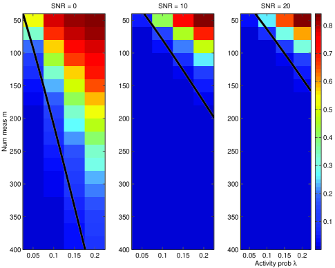
Figure 1: SequOMP with power shaping: Each colored bar represents the SequOMP algorithm’s missed detection probability as a function of the number of measurements $m$, with different bars showing different activity probabilities $\lambda$ and SNR levels. The missed detection probabilities were estimated with 1000 Monte Carlo trials. The number of users is set to $n=100$, the false alarm probability is $p_{\rm FA}=10^{-3}$. The power shaping is performed with a leakage fraction of $\theta=0.1$. The dark black line shows the theoretical number of measurements $m$ required in Theorem 1 with $\gamma=\gamma(\theta)$ in (38c).

The dark line in Fig. 1 represents the number of measurements $m$ for which Theorem 1 would theoretically guarantee reliable detection of the support at infinite block lengths. To apply the theorem, we used the MSINR $\gamma=\gamma(\theta)$ in (38c). At the block lengths considered in this simulation, the missed detection probability at the theoretical sufficient condition is small, typically between 2 and 10%. Thus, even at moderate block lengths, the theoretical bound in Theorem 1 can provide a good estimate for the number of measurements for reliable detection.

V-C SequOMP vs. Thresholding

Fig. 2 compares the performances of thresholding and SequOMP with power shaping. In the simulations, $n=100$, $\lambda=0.1$, and the total SNR is 20 dB. The number of measurements $m$ was varied, and for each $m$, the missed detection probability was estimated with 1000 Monte Carlo trials.

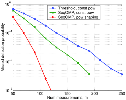
Figure 2: Missed detection probabilities for various detection methods and power profiles. The number of users is $n=100$, $\mbox{\scriptsize SNR}=20\,{\rm dB}$, the activity probability is $\lambda=0.1$, and the false alarm rate is $p_{\rm FA}=10^{-3}$. For the SequOMP algorithm with power shaping, the leakage fraction was set to $\theta=0.1$.

As expected, thresholding requires the most number of measurements. For a missed detection rate of 1%, Fig. 2 shows that thresholding requires approximately $m\approx 210$ measurements. In this simulation of thresholding, the power profile is constant. Employing SequOMP but keeping the power profile constant decreases the number of measurements somewhat to $m\approx 170$ for a 1% missed detection rate. However, using SequOMP with power shaping decreases the number of measurements by more than a factor of two to $m\approx 95$. Thus, at least at high SNRs, SequOMP may provide significant gains over simple thresholding.

V-D OMP with Power Shaping

As discussed earlier, although SequOMP can provide gains over thresholding, its performance is typically worse than OMP, even if SequOMP is used with power shaping. (Our interest in SequOMP is that it is simple to analyze.)

While we do not have any analytical result, the simulation in Fig. 3 shows that power shaping provides gains with OMP as well. Specifically, when the power profile is constant, $m\approx 85$ measurements are needed for a missed detection probability of 1%. This number is slightly lower than that required by SequOMP, even when SequOMP uses power shaping. When OMP is used with power shaping, the number of measurements decreases to $m\approx 65$.

Figure 3: Power shaping with OMP. Plotted is the missed detection probabilities with OMP using a constant power profile, and power shaping wiht a leakage fraction set to $\theta=0.1$. Other simulation assumptions are identical to Fig. 2.

VI Conclusions

Methods such as OMP and lasso, which are widely used in sparse signal support detection problems, exhibit advantages over thresholding but still fall far short of the performance of optimal (ML) detection at high SNRs. Analysis of the SequOMP algorithm has shown that knowledge of conditional rank of signal components enables performance similar to OMP and lasso at a lower complexity. Furthermore, in the most favorable situations, conditional rank knowledge changes the fundamental scaling of performance with SNR so that performance no longer saturates with SNR.

Proof of Theorem 1

-A Proof Outline

At a high level, the proof of Theorem 1 is similar to the proof of [4, Thm. 2], the thresholding condition (17). One of the difficulties in the proof is to handle the dependence between random events at different iterations of the SequOMP algorithm. To avoid this difficulty, we first show an equivalence between the success of SequOMP and an alternative sequence of events that is easier to analyze. After this simplification, small modifications handle the cancellations of detected vectors.

Fix $n$ and define

$$I_{\rm true}(j)=\left\{~{}\ell~{}:~{}\ell\in I_{\rm true},\ell\leq j\right\},$$

which is the set of elements of the true support with indices $\ell\leq j$. Observe that $I_{\rm true}(0)=\{\emptyset\}$ and $I_{\rm true}(n)=I_{\rm true}$.

Let $\mathbf{P}_{\rm true}(j)$ be the projection operator onto the orthogonal complement of $\{\mathbf{a}_{\ell},~{}\ell\in I_{\rm true}(j-1)\}$, and define

$$\rho_{\rm true}(j)=\frac{|\mathbf{a}_{j}^{\prime}\mathbf{P}_{\rm true}(j)\mathbf{y}|^{2}}{\|\mathbf{P}_{\rm true}(j)\mathbf{a}_{j}\|^{2}\|\mathbf{P}_{\rm true}(j)\mathbf{y}\|^{2}}.$$ (39)

A simple induction argument shows that SequOMP correctly detects the support if and only if, at each iteration $j$, the variables $\hat{I}(j)$, $\mathbf{P}(j)$ and $\rho(j)$ defined in the algorithm are equal to $I_{\rm true}(j)$, $\mathbf{P}_{\rm true}(j)$ and $\rho_{\rm true}(j)$, respectively. Therefore, if we define

$$\hat{I}=\left\{~{}j~{}:~{}\rho_{\rm true}(j)>\mu~{}\right\},$$ (40)

then SequOMP correctly detects the support if and only if $\hat{I}=I_{\rm true}$. In particular,

$$p_{\rm err}(n)=\Pr\left(\hat{I}\neq I_{\rm true}\right).$$

To prove that $p_{\rm err}(n)\rightarrow 0$ it suffices to show that there exists a sequence of threshold levels $\mu(n)$ such the following two limits

$$\liminf_{n\rightarrow\infty}\min_{j\in I_{\rm true}(n)}\frac{\rho_{\rm true}(j)}{\mu}>1,$$ (41)

$$\limsup_{n\rightarrow\infty}\max_{j\not\in I_{\rm true}(n)}\frac{\rho_{\rm true}(j)}{\mu}<1,$$ (42)

hold in probability. The first limit (41) ensures that all the components in the true support will not be missed and will be called the zero missed detection condition. The second limit (42) ensures that all the components not in the true support will not be falsely detected and will be called the zero false alarm condition.

Set the sequence of threshold levels as follows. Since $\delta>0$, we can find an $\epsilon>0$ such that

$$(1+\delta)\geq(1+\epsilon)^{2}.$$ (43)

For each $n$, let the threshold level be

$$\mu=(1+\epsilon)\frac{\log(n(1-\lambda))}{m-\lambda n}.$$ (44)

The asymptotic lack of missed detections and false alarms with these thresholds are proven in Appendices -D and -E, respectively. In preparation for these sections, Appendix -B reviews some facts concerning tail bounds on Chi-squared and Beta random variables and Appendix -C performs some preliminary computations.

-B Chi-Squared and Beta Random Variables

The proof requires a number of simple facts concerning chi-squared and beta random variables. These variables are reviewed in [37]. We will omit all the proofs in this subsections as they can be proved along the lines of the calculations in [4].

A random variable $u$ has a chi-squared distribution with $r$ degrees of freedom if it can be written as $u=\sum_{i=1}^{r}z_{i}^{2}$, where $z_{i}$ are i.i.d. ${\mathcal{N}}(0,1)$.

Lemma 1

Suppose $\mathbf{x}\in{\mathbb{R}}^{r}$ has a Gaussian distribution ${\mathcal{N}}(0,\sigma^{2}I_{r})$. Then:

• $\|\mathbf{x}\|^{2}/\sigma^{2}$ is chi-squared with $r$ degrees of freedom; and

• if $\mathbf{y}$ is any other $r$-dimensional random vector that is nonzero with probability one and independent of $\mathbf{x}$, then the variable

  $$u=\frac{|\mathbf{x}^{\prime}\mathbf{y}|^{2}}{\sigma^{2}\|\mathbf{y}\|^{2}}$$

  is a chi-squared random variable with one degree of freedom.

The following two lemmas provide standard tail bounds.

Lemma 2

Suppose that for each $n$, $\{\mathbf{x}_{j}^{(n)}\}_{j=1}^{n}$ is a set of Gaussian random vectors with each $\mathbf{x}_{j}^{(n)}$ spherically symmetric in an $m_{j}(n)$-dimensional space. The variables may be dependent. Suppose also that $\mathbf{E}\|\mathbf{x}_{j}^{(n)}\|^{2}=1$ and

$$\lim_{n\rightarrow\infty}\log(n)/m_{\rm min}(n)=0$$

where

$$m_{\rm min}(n)=\min_{j=1,\ldots,n}m_{j}(n).$$

Then the limits

$$\lim_{n\rightarrow\infty}\max_{j=1,\ldots,n}\|\mathbf{x}_{j}^{(n)}\|^{2}=\lim_{n\rightarrow\infty}\min_{j=1,\ldots,n}\|\mathbf{x}_{j}^{(n)}\|^{2}=1$$

hold in probability.

Lemma 3

Suppose that for each $n$, $\{u_{j}^{(n)}\}_{j=1}^{n}$ is a set of chi-squared random variables, each with one degree of freedom. The variables may be dependent. Then

$$\limsup_{n\rightarrow\infty}\max_{j=1,\ldots,n}\frac{u_{j}^{(n)}}{2\log(n)}\leq 1,$$ (45)

where the limit is in probability.

The final two lemmas concern certain beta distributed random variables. A real-valued scalar random variable $w$ follows a $\mbox{Beta}(r,s)$ distribution if it can be written as $w=u_{r}/(u_{r}+v_{s})$, where the variables $u_{r}$ and $v_{s}$ are independent chi-squared random variables with $r$ and $s$ degrees of freedom, respectively. The importance of the beta distribution is given by the following lemma.

Lemma 4

Suppose $\mathbf{x}$ and $\mathbf{y}$ are independent random $r$-dimensional random vectors with $\mathbf{x}$ being spherically-symmetrically distributed in ${\mathbb{R}}^{r}$ and $\mathbf{y}$ having any distribution that is nonzero with probability one. Then the random variable

$$w=\frac{|\mathbf{x}^{\prime}\mathbf{y}|^{2}}{\|\mathbf{x}\|^{2}\|\mathbf{y}\|^{2}}$$

is independent of $\mathbf{x}$ and follows a $\mbox{Beta}(1,r-1)$ distribution.

The following lemma provides a simple expression for the maxima of certain beta distributed variables.

Lemma 5

For each $n$, suppose $\{w_{j}^{(n)}\}_{j=1}^{n}$ is a set of random variables with $w_{j}^{(n)}$ having a $\mbox{Beta}(1,m_{j}(n)-1)$ distribution. Suppose that

$$\lim_{n\rightarrow\infty}\log(n)/m_{\rm min}(n)=0,\ \ \ \lim_{n\rightarrow\infty}m_{\rm min}(n)=\infty$$ (46)

where

$$m_{\rm min}(n)=\min_{j=1,\ldots,n}m_{j}(n).$$

Then,

$$\limsup_{n\rightarrow\infty}\max_{j=1,\ldots,n}\frac{m_{j}(n)}{2\log(n)}w_{j}^{(n)}\leq 1$$

in probability.

-C Preliminary Computations and Technical Lemmas

We first need to prove a number of simple but technical bounds. We begin by considering the dimension $m_{i}$ defined as

$$m_{i}=\mathop{\mathrm{dim}}(\mathop{\mathrm{range}}(\mathbf{P}_{\rm true}(i))).$$ (47)

Our first lemma computes the limit of this dimension.

Lemma 6

The following limit

$$\lim_{n\rightarrow\infty}\min_{i=1,\ldots,n}\frac{m_{i}}{m-\lambda n}=1$$ (48)

holds in probability and almost surely. The deterministic limits

$$\lim_{n\rightarrow\infty}\frac{\log(\lambda n)}{m-\lambda n}=\lim_{n\rightarrow\infty}\frac{\log((1-\lambda)n)}{m-\lambda n}=0$$ (49)

also hold.

Proof:

Recall that $\mathbf{P}_{\rm true}(i)$ is the projection onto the orthogonal complement of the vectors $\mathbf{a}_{j}$ with $j\in I_{\rm true}(i-1)$. With probability one, these vectors will be linearly independent, so $\mathbf{P}_{\rm true}(i)$ will have dimension $m-|I_{\rm true}(i-1)|$. Since $I_{\rm true}(i)$ is increasing with $i$,

$$\min_{i=1,\ldots,n}m_{i} = m-\max_{i=1,\ldots,n}|I_{\rm true}(i-1)|$$ (50)

$$= m-|I_{\rm true}(n-1)|.$$

Since each user is active with probability $\lambda$ and the activities of the users are independent, the law of large numbers shows that

$$\lim_{n\rightarrow\infty}\frac{|I_{\rm true}(n-1)|}{\lambda(n-1)}=1$$

in probability and almost surely. Combining this with (50) shows (48).

We next show (49). Since the hypothesis of the theorem requires that $\lambda n$, $(1-\lambda)n$ and $m-\lambda n$ all approach infinity, the fractions in (49) are eventually positive. Also, from (15), $L(\lambda,n)<\max\{\log(\lambda n),\log((1-\lambda)n)\}$. Therefore, from (26),

$$\frac{1}{m-\lambda n}\max\{\log(\lambda n),\log((1-\lambda)n)\}$$

$$\leq \frac{\gamma}{2L(\lambda,n)}\max\{\log(\lambda n),\log((1-\lambda)n)\}\leq\frac{\gamma}{2}\rightarrow 0,$$

where the last step is from the hypothesis of the theorem. ∎

Next, for each $i=1,\ldots,n$, define the residual vector,

$$\mathbf{e}_{i}=\mathbf{P}_{\rm true}(i)(\mathbf{y}-\mathbf{a}_{i}x_{i}).$$ (51)

Observe that

$$\mathbf{e}_{i} = \mathbf{P}_{\rm true}(i)(\mathbf{y}-\mathbf{a}_{i}x_{i})$$ (52)

$$\stackrel{{\scriptstyle(a)}}{{=}} \mathbf{P}_{\rm true}(i)\left(\mathbf{d}+\sum_{j\neq i}\mathbf{a}_{j}x_{j}\right)$$

$$\stackrel{{\scriptstyle(b)}}{{=}} \mathbf{P}_{\rm true}(i)\left(\mathbf{d}+\sum_{j>i}\mathbf{a}_{j}x_{j}\right)$$

where (a) follows from (1) and (b) follows from the fact that $\mathbf{P}_{\rm true}(i)$ is the projection onto the orthogonal complement of the span of all vectors $\mathbf{a}_{j}$ with $j<i$ and $x_{j}\neq 0$.

The next lemma shows that the power of the residual vector is described by the random variable

$$\sigma^{2}(i)=1+\sum_{j=i+1}^{n}|x_{j}|^{2}.$$ (53)

Lemma 7

For all $i=1,\ldots,n$, the residual vector $\mathbf{e}_{i}$, conditioned on the modulation vector $\mathbf{x}$ and projection $\mathbf{P}_{\rm true}(i)$, is a spherically symmetric Gaussian in the range space of $\mathbf{P}_{\rm true}(i)$ with total variance

$$\mathbf{E}\left(\|\mathbf{e}_{i}\|^{2}\mid\mathbf{x}\right)=\frac{m_{i}}{m}\sigma^{2}(i),$$ (54)

where $m_{i}$ and $\sigma^{2}(i)$ are defined in (47) and (53), respectively.

Proof:

Let

$$\mathbf{v}_{i}=\mathbf{d}+\sum_{j>i}\mathbf{a}_{j}x_{j},$$

so that $\mathbf{e}_{i}=\mathbf{P}_{\rm true}(i)\mathbf{v}_{i}$. Since the vectors $\mathbf{a}_{j}$ and $\mathbf{d}$ have Gaussian ${\mathcal{N}}(0,1/mI_{m})$ distributions, for a given vector $\mathbf{x}$, $\mathbf{v}_{i}$ must be a zero-mean white Gaussian vector with total variance $\mathbf{E}\|\mathbf{v}_{i}\|^{2}=\sigma^{2}(i)$. Also, since the operator $\mathbf{P}_{\rm true}(i)$ is a function of the components $x_{\ell}$ and vectors $\mathbf{a}_{\ell}$ for $\ell<i$, $\mathbf{P}_{\rm true}(i)$ is independent of the vectors $\mathbf{d}$ and $\mathbf{a}_{j}$, $j>i$, and therefore independent of $\mathbf{v}_{i}$. Since $\mathbf{P}_{\rm true}(i)$ is a projection from an $m$-dimensional space to an $m_{i}$-dimensional space, $\mathbf{e}_{i}$, conditioned on the modulation vector $\mathbf{x}$, must be spherically symmetric Gaussian in the range space of $\mathbf{P}_{\rm true}(i)$ with total variance satisfying (54). ∎

Our next lemma requires the following version of the well-known Hoeffding’s inequality.

Lemma 8 (Hoeffding’s Inequality)

Suppose $z$ is the sum

$$z=z_{0}+\sum_{i=1}^{r}z_{i}$$

where $z_{0}$ is a constant and the variables $z_{i}$ are independent random variables that are almost surely bounded in some interval $z_{i}\in[a_{i},b_{i}]$. Then, for all $\epsilon>0$,

$$\Pr\left(z-\mathbf{E}(z)\geq\epsilon\right)\leq\exp\left(\frac{-2\epsilon^{2}}{C}\right),$$

where

$$C=\sum_{i=1}^{r}(b_{i}-a_{i})^{2}.$$

Proof:

See [38]. ∎

Lemma 9

Under the assumptions of Theorem 1, the limit

$$\limsup_{n\rightarrow\infty}\max_{i=1,\ldots,n}\frac{\sigma^{2}(i)}{\widehat{\sigma}^{2}(i)}\leq 1$$

holds in probability.

Proof:

Let $z(i)=\sigma^{2}(i)/\widehat{\sigma}^{2}(i)$. From the definition of $\sigma^{2}(i)$ in (53), we can write

$$z(i)=\frac{1}{\widehat{\sigma}^{2}(i)}+\sum_{j=i+1}^{n}z(i,j),$$

where $z(i,j)=|x_{j}|^{2}/\widehat{\sigma}^{2}(i)$ for $j>i$.

Now recall that in the problem formulation, each user is active with probability $\lambda$, with power $|x_{j}|^{2}=p_{j}$ conditioned on when the user being active. Also, the activities of different users are independent, and the conditional powers $p_{j}$ are treated as deterministic quantities. Therefore, the variables $z(i,j)$ are independent with

$$z(i,j)=\left\{\begin{array}[]{ll}p_{j}/\widehat{\sigma}^{2}(i),&\mbox{with probability $\lambda$;}\\ 0,&\mbox{with probability $1-\lambda$},\end{array}\right.$$

for $j>i$. Combining this with the definition of $\widehat{\sigma}^{2}(i)$ in (24), we see that

$$\mathbf{E}(z(i))=\frac{1}{\widehat{\sigma}^{2}(i)}\left(1+\lambda\sum_{j=i+1}^{n}p_{j}\right)=1.$$

Also, for each $j>i$, we have the bound

$$z(i,j)\in[0,p_{j}/\widehat{\sigma}^{2}(i)].$$

So for use in Hoeffding’s Inequality (Lemma 8), define

$$C=C(i,n)=\widehat{\sigma}^{-4}(i)\sum_{j=i+1}^{n}p_{j}^{2},$$

where dependence of the power profile and $\widehat{\sigma}(i)$ on $n$ is implicit. Now define

$$c_{n}=\max_{i=1,\ldots,n}\log(n)C(i,n),$$

so that $C(i,n)\leq c_{n}/\log(n)$ for all $i$. Hoeffding’s Inequality (Lemma 8) now shows that for all $i<n$,

$$\Pr(z(i)\geq 1+\epsilon) \leq \exp\left(-2\epsilon^{2}/C(i,n)\right)$$

$$\leq \exp\left(-2\epsilon^{2}\log(n)/c_{n}\right).$$

Using the union bound,

$$\lim_{n\rightarrow\infty}\Pr\left(\max_{j=1,\ldots,n}z(i)>1+\epsilon\right)$$

$$\leq \lim_{n\rightarrow\infty}n\exp\left(-\frac{2\epsilon^{2}\log(n)}{c_{n}}\right)$$

$$= \lim_{n\rightarrow\infty}n^{1-2\epsilon^{2}/c_{n}}=0.$$

The final step is due to the fact that the technical condition (25) in the theorem implies $c_{n}\rightarrow 0$. This proves the lemma. ∎

-D Missed Detection Probability

Consider any $j\in I_{\rm true}$. Using (51) to rewrite (39) along with some algebra shows

$$\rho_{\rm true}(j) = \frac{|\mathbf{a}_{j}^{\prime}\mathbf{P}_{\rm true}(j)\mathbf{y}|^{2}}{\|\mathbf{P}_{\rm true}(j)\mathbf{a}\|^{2}\|\mathbf{P}_{\rm true}(j)\mathbf{y}_{j}\|^{2}}$$ (55)

$$= \frac{|\mathbf{a}_{j}^{\prime}(x_{j}\mathbf{P}_{\rm true}(j)\mathbf{a}_{j}+\mathbf{e}_{j})|^{2}}{\|\mathbf{P}_{\rm true}(j)\mathbf{a}_{j}\|^{2}\|x_{j}\mathbf{P}_{\rm true}(j)\mathbf{a}_{j}+\mathbf{e}_{j}\|^{2}}$$

$$\geq \frac{s_{j}-2\sqrt{z_{j}s_{j}}+z_{j}}{s_{j}+2\sqrt{z_{j}s_{j}}+1},$$

where

$$s_{j} = \frac{|x_{j}|^{2}\|\mathbf{P}_{\rm true}(j)\mathbf{a}_{j}\|^{2}}{\|\mathbf{e}_{j}\|^{2}},$$ (56)

$$z_{j} = \frac{|\mathbf{a}_{j}^{\prime}\mathbf{P}_{\rm true}(j)\mathbf{e}_{j}|^{2}}{\|\mathbf{P}_{\rm true}(j)\mathbf{a}_{j}\|^{2}\|\mathbf{e}_{j}\|^{2}}.$$ (57)

Define

$$s_{\rm min}=\min_{j\in I_{\rm true}}s_{j},\ \ \ s_{\rm max}=\max_{j\in I_{\rm true}}z_{j}.$$

We will now bound $s_{\rm min}$ from below and $s_{\rm max}$ from above.

We first start with $s_{\rm min}$. Conditional on $\mathbf{x}$ and $\mathbf{P}_{\rm true}(j)$, Lemma 7 shows that each $\mathbf{e}_{j}$ is a spherically-symmetrically distributed Gaussian on the $m_{j}$-dimensional range space of $\mathbf{P}_{\rm true}(j)$. Since there are asymptotically $\lambda n$ elements in $I_{\rm true}$, Lemma 2 along with (49) show that

$$\lim_{n\rightarrow\infty}\max_{j\in I_{\rm true}}\frac{m}{m_{j}\sigma^{2}(j)}\|\mathbf{e}_{j}\|^{2}=1,$$ (58)

where the limit is in probability. Similarly, $\mathbf{P}_{\rm true}(j)\mathbf{a}_{j}$ is also a spherically-symmetrically distributed Gaussian in the range space of $\mathbf{P}_{\rm true}(j)$. Since $\mathbf{P}_{\rm true}(j)$ is a projection from an $m$-dimensional space to a $m_{j}$-dimensional space and $\mathbf{E}\|\mathbf{a}_{j}\|^{2}=1$, we have that $\mathbf{E}\|\mathbf{P}_{\rm true}(j)\mathbf{a}_{j}\|^{2}=m_{j}/m$. Therefore, Lemma 2 along with (49) show that

$$\lim_{n\rightarrow\infty}\min_{j\in I_{\rm true}}\frac{m}{m_{j}}\|\mathbf{P}_{\rm true}(j)\mathbf{e}_{j}\|^{2}=1.$$ (59)

Taking the limit (in probability) of $s_{\rm min}$,

$$\liminf_{n\rightarrow\infty}\frac{s_{\rm min}}{\gamma} = \liminf_{n\rightarrow\infty}\min_{j\in I_{\rm true}}\frac{s_{j}}{\gamma}$$ (60)

$$\stackrel{{\scriptstyle(a)}}{{=}} \liminf_{n\rightarrow\infty}\min_{j\in I_{\rm true}}\frac{|x_{j}|^{2}\|\mathbf{P}_{\rm true}(j)\mathbf{a}_{j}\|^{2}}{\gamma\|\mathbf{e}_{j}\|^{2}}$$

$$\stackrel{{\scriptstyle(b)}}{{=}} \liminf_{n\rightarrow\infty}\min_{j\in I_{\rm true}}\frac{|x_{j}|^{2}}{\gamma\sigma^{2}(j)}$$

$$\stackrel{{\scriptstyle(c)}}{{=}} \liminf_{n\rightarrow\infty}\min_{j\in I_{\rm true}}\frac{p_{j}}{\gamma\sigma^{2}(j)}$$

$$\stackrel{{\scriptstyle(d)}}{{\geq}} \liminf_{n\rightarrow\infty}\min_{j\in I_{\rm true}}\frac{p_{j}}{\gamma\widehat{\sigma}^{2}(j)}$$

$$\stackrel{{\scriptstyle(e)}}{{\geq}} 1,$$

where (a) follows from (56); (b) follows from (58) and (59); (c) follows from (21); (d) follows from Lemma 9; and (e) follows from (23).

We next consider $s_{\rm max}$. Conditional on $\mathbf{P}_{\rm true}(j)$, the vectors $\mathbf{P}_{\rm true}(j)\mathbf{a}_{j}$ and $\mathbf{e}_{j}$ are independent spherically-symmetric Gaussians in the range space of $\mathbf{P}_{\rm true}(j)$. It follows from Lemma 4 that each $z_{j}$ is a $\mbox{Beta}(1,m_{j}-1)$ random variable. Since there are asymptotically $\lambda n$ elements in $I_{\rm true}$, Lemma 5 along with (48) and (49) show that

$${\limsup_{n\rightarrow\infty}\frac{m-\lambda n}{2\log(\lambda n)}s_{\rm max}}=\limsup_{n\rightarrow\infty}\frac{m-\lambda n}{2\log(\lambda n)}\max_{j\in I_{\rm true}}z_{j}\leq 1.$$ (61)

The above analysis shows that for any $j\in I_{\rm true}$,

$$\liminf_{n\rightarrow\infty}\min_{j\in I_{\rm true}}\frac{1}{\sqrt{\mu}}(\sqrt{s_{j}}-\sqrt{z_{j}})$$ (62)

$$\stackrel{{\scriptstyle(a)}}{{\geq}} \liminf_{n\rightarrow\infty}\frac{1}{\sqrt{\mu}}(\sqrt{s_{\rm min}}-\sqrt{s_{\rm max}})$$

$$\stackrel{{\scriptstyle(b)}}{{\geq}} \liminf_{n\rightarrow\infty}\frac{1}{\sqrt{\mu}}\left(\sqrt{\gamma}-\sqrt{\frac{2\log(\lambda n)}{m-\lambda n}}\right)$$

$$\geq \liminf_{n\rightarrow\infty}\sqrt{\frac{1+\delta}{\mu}}\left(\sqrt{\frac{\gamma}{1+\delta}}-\sqrt{\frac{2\log(\lambda n)}{m-\lambda n}}\right)$$

$$\stackrel{{\scriptstyle(c)}}{{\geq}} \liminf_{n\rightarrow\infty}\sqrt{\frac{2(1+\delta)}{(m-\lambda n)\mu}}\left(\sqrt{L(\lambda,n)}-\sqrt{\log(\lambda n)}\right)$$

$$\stackrel{{\scriptstyle(d)}}{{=}} \liminf_{n\rightarrow\infty}\sqrt{\frac{2(1+\delta)\log(n(1-\lambda))}{(m-\lambda n)\mu}}$$

$$\stackrel{{\scriptstyle(e)}}{{=}} \liminf_{n\rightarrow\infty}\sqrt{\frac{1+\delta}{1+\epsilon}}\ \stackrel{{\scriptstyle(f)}}{{\geq}}\ \sqrt{1+\epsilon}$$

where (a) follows from the definitions of $s_{\rm min}$ and $s_{\rm max}$; (b) follows from (60) and (61); (c) follows from (26); (d) follows from (15); (e) follows from (44); and (f) follows from (43). Therefore, starting with (55),

$$\liminf_{n\rightarrow\infty}\min_{j\in I_{\rm true}}\frac{\rho(j)}{\mu}$$

$$\stackrel{{\scriptstyle(a)}}{{\geq}} \liminf_{n\rightarrow\infty}\min_{j\in I_{\rm true}}\frac{1}{\mu}\frac{s_{j}-2\sqrt{z_{j}s_{j}}+z_{j}}{s_{j}+2\sqrt{z_{j}s_{j}}+1}$$

$$= \liminf_{n\rightarrow\infty}\min_{j\in I_{\rm true}}\frac{1}{\mu}\frac{(\sqrt{s_{j}}-\sqrt{z_{j}})^{2}}{s_{j}+2\sqrt{z_{j}s_{j}}+1}$$

$$\stackrel{{\scriptstyle(b)}}{{\geq}} \liminf_{n\rightarrow\infty}\min_{j\in I_{\rm true}}\frac{1+\epsilon}{s_{j}+2\sqrt{z_{j}s_{j}}+1}$$

$$\stackrel{{\scriptstyle(c)}}{{\geq}} \liminf_{n\rightarrow\infty}\min_{j\in I_{\rm true}}\frac{1+\epsilon}{s_{j}+2\sqrt{s_{j}}+1}$$

$$\geq \liminf_{n\rightarrow\infty}\min_{j\in I_{\rm true}}\frac{1+\epsilon}{s_{\rm min}+2\sqrt{s_{\rm min}}+1}$$

$$\stackrel{{\scriptstyle(d)}}{{\geq}} \liminf_{n\rightarrow\infty}\min_{j\in I_{\rm true}}\frac{1+\epsilon}{(\sqrt{\gamma}+1)^{2}}\stackrel{{\scriptstyle(e)}}{{=}}1+\epsilon,$$

where (a) follows from (55); (b) follows from (62); (c) follows from the fact that $z_{j}\in[0,1]$ (it is a Beta distributed random variable); (d) follows from (60); and (e) follows from the condition of the hypothesis of the theorem that $\gamma\rightarrow 0$. This proves the first requirement, condition (41).

-E False Alarm Probability

Now consider any index $j\not\in I_{\rm true}$. This implies that $x_{j}=0$ and therefore (51) shows that

$$\mathbf{P}_{\rm true}(j)\mathbf{y}=\mathbf{e}_{j}.$$

Hence from (39),

$$\rho_{\rm true}(j)=\frac{|\mathbf{a}_{j}^{\prime}\mathbf{e}|^{2}}{\|\mathbf{P}_{\rm true}(j)\mathbf{a}\|^{2}\|\mathbf{e}_{j}\|^{2}}=z_{j}$$ (63)

where $z_{j}$ is defined in (57). From the discussion above, each $z_{j}$ has the $\mbox{Beta}(2,m_{j}-2)$ distribution. Since there are asymptotically $(1-\lambda)n$ elements in $I_{\rm true}^{c}$, the conditions (48) and (49) along with Lemma 5 show that the limit

$$\limsup_{n\rightarrow\infty}\max_{j\not\in I_{\rm true}}\frac{m-\lambda n}{2\log(n(1-\lambda))}z_{j}\leq 1$$ (64)

holds in probability. Therefore,

$$\limsup_{n\rightarrow\infty}\max_{j\not\in I_{\rm true}}\frac{1}{\mu}\rho_{\rm true}(j)$$

$$\stackrel{{\scriptstyle(a)}}{{=}} \limsup_{n\rightarrow\infty}\max_{j\not\in I_{\rm true}}\frac{1}{\mu}z_{j}$$

$$\stackrel{{\scriptstyle(b)}}{{=}} \limsup_{n\rightarrow\infty}\max_{j\not\in I_{\rm true}}\frac{m-\lambda n}{(1+\epsilon)\log(n(1-\lambda))}z_{j}$$

$$\stackrel{{\scriptstyle(c)}}{{\leq}} \frac{1}{1+\epsilon}$$

where (a) follows from (63); (b) follows from (44); and (c) follows from (64). This proves (42) and thus completes the proof of the theorem.

References

- [1] A. K. Fletcher, S. Rangan, and V. K. Goyal, “A sparsity detection framework for on–off random access channels,” in Proc. IEEE Int. Symp. Inform. Theory, Seoul, Korea, Jun.–Jul. 2009, pp. 169–173.
- [2] M. J. Wainwright, “Information-theoretic limits on sparsity recovery in the high-dimensional and noisy setting,” IEEE Trans. Inform. Theory, vol. 55, no. 12, pp. 5728–5741, Dec. 2009.
- [3] ——, “Sharp thresholds for high-dimensional and noisy sparsity recovery using -constrained quadratic programming (lasso),” IEEE Trans. Inform. Theory, vol. 55, no. 5, pp. 2183–2202, May 2009.
- [4] A. K. Fletcher, S. Rangan, and V. K. Goyal, “Necessary and sufficient conditions for sparsity pattern recovery,” IEEE Trans. Inform. Theory, vol. 55, no. 12, pp. 5758–5772, Dec. 2009.
- [5] B. K. Natarajan, “Sparse approximate solutions to linear systems,” SIAM J. Computing, vol. 24, no. 2, pp. 227–234, Apr. 1995.
- [6] S. G. Mallat and Z. Zhang, “Matching pursuits with time-frequency dictionaries,” IEEE Trans. Signal Process., vol. 41, no. 12, pp. 3397–3415, Dec. 1993.
- [7] S. Chen, S. A. Billings, and W. Luo, “Orthogonal least squares methods and their application to non-linear system identification,” Int. J. Control, vol. 50, no. 5, pp. 1873–1896, Nov. 1989.
- [8] Y. C. Pati, R. Rezaiifar, and P. S. Krishnaprasad, “Orthogonal matching pursuit: Recursive function approximation with applications to wavelet decomposition,” in Conf. Rec. 27th Asilomar Conf. Sig., Sys., & Comput., vol. 1, Pacific Grove, CA, Nov. 1993, pp. 40–44.
- [9] G. Davis, S. Mallat, and Z. Zhang, “Adaptive time-frequency decomposition,” Optical Eng., vol. 33, no. 7, pp. 2183–2191, Jul. 1994.
- [10] D. Needell and J. A. Tropp, “CoSaMP: Iterative signal recovery from incomplete and inaccurate samples,” Appl. Comput. Harm. Anal., vol. 26, no. 3, pp. 301–321, May 2009.
- [11] W. Dai and O. Milenkovic, “Subspace pursuit for compressive sensing signal reconstruction,” IEEE Trans. Inform. Theory, vol. 55, no. 5, pp. 2230–2249, May 2009.
- [12] S. S. Chen, D. L. Donoho, and M. A. Saunders, “Atomic decomposition by basis pursuit,” SIAM J. Sci. Comp., vol. 20, no. 1, pp. 33–61, 1999.
- [13] R. Tibshirani, “Regression shrinkage and selection via the lasso,” J. Royal Stat. Soc., Ser. B, vol. 58, no. 1, pp. 267–288, 1996.
- [14] E. J. Candès and T. Tao, “The Dantzig selector: Statistical estimation when is much larger than ,” Ann. Stat., vol. 35, no. 6, pp. 2313–2351, Dec. 2007.
- [15] D. L. Donoho, M. Elad, and V. N. Temlyakov, “Stable recovery of sparse overcomplete representations in the presence of noise,” IEEE Trans. Inform. Theory, vol. 52, no. 1, pp. 6–18, Jan. 2006.
- [16] J. A. Tropp, “Greed is good: Algorithmic results for sparse approximation,” IEEE Trans. Inform. Theory, vol. 50, no. 10, pp. 2231–2242, Oct. 2004.
- [17] ——, “Just relax: Convex programming methods for identifying sparse signals in noise,” IEEE Trans. Inform. Theory, vol. 52, no. 3, pp. 1030–1051, Mar. 2006.
- [18] E. J. Candès, J. Romberg, and T. Tao, “Robust uncertainty principles: Exact signal reconstruction from highly incomplete frequency information,” IEEE Trans. Inform. Theory, vol. 52, no. 2, pp. 489–509, Feb. 2006.
- [19] D. L. Donoho, “Compressed sensing,” IEEE Trans. Inform. Theory, vol. 52, no. 4, pp. 1289–1306, Apr. 2006.
- [20] E. J. Candès and T. Tao, “Near-optimal signal recovery from random projections: Universal encoding strategies?” IEEE Trans. Inform. Theory, vol. 52, no. 12, pp. 5406–5425, Dec. 2006.
- [21] S. Rangan, A. Fletcher, and V. K. Goyal, “Asymptotic analysis of MAP estimation via the replica method and applications to compressed sensing,” IEEE Trans. Inform. Theory, 2011, to appear; available as arXiv:0906.3234v1 [cs.IT].
- [22] D. L. Donoho and J. Tanner, “Counting faces of randomly-projected polytopes when the projection radically lowers dimension,” J. Amer. Math. Soc., vol. 22, no. 1, pp. 1–53, Jan. 2009.
- [23] S. Sarvotham, D. Baron, and R. G. Baraniuk, “Measurements vs. bits: Compressed sensing meets information theory,” in Proc. 44th Ann. Allerton Conf. on Commun., Control and Comp., Monticello, IL, Sep. 2006.
- [24] A. K. Fletcher, S. Rangan, and V. K. Goyal, “Rate-distortion bounds for sparse approximation,” in IEEE Statist. Sig. Process. Workshop, Madison, WI, Aug. 2007, pp. 254–258.
- [25] G. Reeves, “Sparse signal sampling using noisy linear projections,” Univ. of California, Berkeley, Dept. of Elec. Eng. and Comp. Sci., Tech. Rep. UCB/EECS-2008-3, Jan. 2008.
- [26] M. Akçakaya and V. Tarokh, “Shannon-theoretic limits on noisy compressive sampling,” IEEE Trans. Inform. Theory, vol. 56, no. 1, pp. 492–504, Jan. 2010.
- [27] J. A. Tropp and A. C. Gilbert, “Signal recovery from random measurements via orthogonal matching pursuit,” IEEE Trans. Inform. Theory, vol. 53, no. 12, pp. 4655–4666, Dec. 2007.
- [28] A. K. Fletcher and S. Rangan, “Orthogonal matching pursuit from noisy measurements: A new analysis,” in Proc. Neural Information Process. Syst., Y. Bengio, D. Schuurmans, J. Lafferty, C. K. I. Williams, and A. Culotta, Eds., Vancouver, Canada, Dec. 2009.
- [29] H. Rauhut, K. Schnass, and P. Vandergheynst, “Compressed sensing and redundant dictionaries,” IEEE Trans. Inform. Theory, vol. 54, no. 5, pp. 2210–2219, May 2008.
- [30] W. Wang, M. J. Wainwright, and K. Ramchandran, “Information-theoretic limits on sparse signal recovery: Dense versus sparse measurement matrices,” IEEE Trans. Inform. Theory, vol. 56, no. 6, pp. 2967–2979, Jun. 2010.
- [31] M. F. Duarte, S. Sarvotham, D. Baron, W. B. Wakin, and R. G. Baraniuk, “Distributed compressed sensing of jointly sparse signals,” in Conf. Rec. Asilomar Conf. on Signals, Syst. & Computers, Pacific Grove, CA, Oct.–Nov. 2005, pp. 1537–1541.
- [32] M. Tipping, “Sparse Bayesian learning and the relevance vector machine,” J. Machine Learning Research, vol. 1, pp. 211–244, Sep. 2001.
- [33] D. Wipf and B. Rao, “Sparse Bayesian learning for basis selection,” IEEE Trans. Signal Process., vol. 52, no. 8, pp. 2153–2164, Aug. 2004.
- [34] P. Schniter, L. C. Potter, and J. Ziniel, “Fast Bayesian matching pursuit: Model uncertainty and parameter estimation for sparse linear models,” IEEE Trans. Signal Process., Aug. 2008, submitted.
- [35] D. Wipf and B. Rao, “Comparing the effects of different weight distributions on finding sparse representations,” in Proc. Neural Information Process. Syst., Vancouver, Canada, Dec. 2006.
- [36] A. Agrawal, J. G. Andrews, J. M. Cioffi, and T. Meng, “Iterative power control for imperfect successive interference cancellation,” IEEE Trans. Wireless Comm., vol. 4, no. 3, pp. 878–884, May 2005.
- [37] M. Evans, N. Hastings, and J. B. Peacock, Statistical Distributions, 3rd ed. New York: John Wiley & Sons, 2000.
- [38] W. Hoeffding, “Probability inequalities for sums of bounded random variables,” J. Amer. Stat. Assoc., vol. 58, no. 301, pp. 13–30, Mar. 1963.