8 (1:13) 2012 1–33 Apr. 8, 2010 Feb. 27, 2012
*Earlier version appeared in TACAS09
Büchi Complementation and Size-Change Termination\rsuper*
Abstract.
We compare tools for complementing nondeterministic Büchi automata with a recent termination-analysis algorithm. Complementation of Büchi automata is a key step in program verification. Early constructions using a Ramsey-based argument have been supplanted by rank-based constructions with exponentially better bounds. In 2001 Lee et al. presented the size-change termination (SCT) problem, along with both a reduction to Büchi automata and a Ramsey-based algorithm. The Ramsey-based algorithm was presented as a more practical alternative to the automata-theoretic approach, but strongly resembles the initial complementation constructions for Büchi automata.
We prove that the SCT algorithm is a specialized realization of the Ramsey-based complementation construction. To do so, we extend the Ramsey-based complementation construction to provide a containment-testing algorithm. Surprisingly, empirical analysis suggests that despite the massive gap in worst-case complexity, Ramsey-based approaches are superior over the domain of SCT problems. Upon further analysis we discover an interesting property of the problem space that both explains this result and provides a chance to improve rank-based tools. With these improvements, we show that theoretical gains in efficiency of the rank-based approach are mirrored in empirical performance.
Key words and phrases:
Büchi Complementation, Model Checking, Formal Verification, Automata, Büchi Automata1991 Mathematics Subject Classification:
D.2.41. Introduction
The automata-theoretic approach to formal program verification reduces questions about program adherence to a specification to questions about language containment. Representing liveness, fairness, or termination properties requires finite automata that operate on infinite words. One automaton, , encodes the behavior of the program, while another automaton, , encodes the formal specification. To ensure adherence, verify that the intersection of with the complement of is empty. Finite automata on infinite words are classified by their acceptance condition and transition structure. We consider here nondeterministic Büchi automata, in which a run is accepting when it visits at least one accepting state infinitely often. For these automata, the complementation problem is known to involve an exponential blowup [25]. Thus the most difficult step in checking containment is constructing the complementary automata .
The first complementation constructions for nondeterministic Büchi automata employed a Ramsey-based combinatorial argument to partition the set of all infinite words into a finite set of omega-regular languages. Proposed by Büchi in 1962 [5], this construction was shown in 1987 by Sistla, Vardi, and Wolper to be implementable with a blow-up of [29]. This brought the complementation problem into singly-exponential blow-up, but left a gap with the lower bound proved by Michel [25].
The gap was tightened in 1988, when Safra described a construction [26]. Work since then has focused on improving the practicality of constructions, either by providing simpler constructions, further tightening the bound [27], or improving the derived algorithms. In 2001, Kupferman and Vardi employed a rank-based analysis of Büchi automata to simplify complementation [23]. Recently, Doyen and Raskin have demonstrated the utility of using a subsumption technique in the rank-based approach, providing a direct universality checker that scales to automata several orders of magnitude larger than previous tools [10].
Separately, in the context of program termination analysis, Lee, Jones, and Ben-Amram presented the size-change termination (SCT) principle in 2001 [24]. This principle states that, for domains with well-founded values, if every infinite computation contains an infinitely decreasing value sequence, then no infinite computation is possible. Lee et al. describe a method of size-change termination analysis and reduce this problem to the containment of two Büchi automata. Stating the lack of efficient Büchi containment solvers, they also propose a Ramsey-based combinatorial solution that captures all possible call sequences in a finite set of graphs. The Lee, Jones, and Ben-Amram (LJB) algorithm was provided as a practical alternative to reducing the verification problem to Büchi containment, but bears a striking resemblance to the 1987 Ramsey-based complementation construction [29].
In this paper we show that the LJB algorithm for deciding SCT [24] is a specialized implementation of the 1987 Ramsey-based complementation construction [29]. Section 2 presents the background and notation for the paper. Section 3 expands the Ramsey-based complementation construction into a containment algorithm, and then presents the proof that the LJB algorithm is a specialized realization of this Ramsey-based containment algorithm. In Section 4, we empirically explore Lee et al.’s intuition that Ramsey-based algorithms are more practical than Büchi complementation tools on SCT problems. Initial experimentation does suggest that Ramsey-based tools are superior on SCT problems. This is surprising, as the worst-case complexity of the LJB algorithm is significantly worse than that of rank-based tools. Investigating this discovery in Section 5, we note that it is natural for SCT problems to be reverse-deterministic, and that for reverse-deterministic problems the worst-case bound for Ramsey-based algorithms matches that of the rank-based approach. This suggests improving the rank-based approach in the face of reverse determinism. Indeed, we find that reverse-deterministic SCT problems have a maximum rank of 2, collapsing the complexity of rank-based complementation to . Revisiting our experiments, we discover that with this improvement rank-based tools are superior on the domain of SCT problems. To further explore the phenomena, we generate a set of non-reverse-deterministic SCT problems from monotonicity constraint systems, a more complex termination problem. We conclude with a discussion in Section 6.
2. Preliminaries
In this section we review the relevant details of the Büchi complementation and size-change termination, introducing along the way the notation used throughout this paper. A nondeterministic Büchi automaton on infinite words is a tuple , where is a finite nonempty alphabet, a finite nonempty set of states, a set of initial states, a set of accepting states, and a nondeterministic transition function. We lift the function to sets of states and words of arbitrary length as follows. Given a set of states , define to be . Inductively, given a set of states : let , and for every word let be defined as .
A run of a Büchi automaton on a word is a infinite sequence such that and, for every , we have . A run is accepting iff for infinitely many . A word is accepted by if there is an accepting run of on . The words accepted by form the language of , denoted by . Correspondingly, a path in from to on a word is a finite sequence such that , , and, for every , we have . A path is accepting if some state in the path is in .
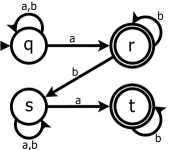
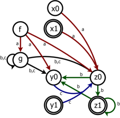
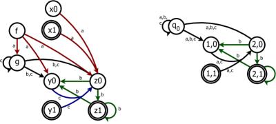
An example automaton is shown in Figure 1, which accepts words with a finite, but non-zero, number of ’s. The automaton waits in and guesses when it has seen the last , transitioning on that to . If the automaton moves to prematurely, it can transition to before it encounters any remaining ’s to continue the run. From , it can guess once again when it has seen the last , transitioning this time to .
A Büchi automaton is contained in a Büchi automaton iff , which can be checked by verifying that the intersection of with the complement of is empty: . We know that the language of an automaton is non-empty iff there are states such that there is a path from to and an accepting path from to itself. The initial path is called the prefix, and the combination of the prefix and cycle is called a lasso [31]. Furthermore, the intersection of two automata can be constructed, having a number of states proportional to the product of the number states of the original automata [6]. Thus, the most computationally demanding step is constructing the complement of . In the formal verification field, existing empirical work has focused on the simplest form of containment testing, universality testing, where is the universal automaton [9, 30].
2.1. Ramsey-Based Universality
When Büchi introduced these automata in 1962, he described a complementation construction involving a Ramsey-based combinatorial argument [5]. We describe an optimized implementation presented in 1987 [29]. To construct the complement of , where , we construct a set whose elements capture the essential behavior of . Each element corresponds to an answer to the following question:
Given a finite nonempty word , for every two states :
- (1)
Is there a path in from to over ?
- (2)
If so, is some such path accepting?
Define , and to be the subset of whose elements, for every , do not contain both and . Each element of is a -arc-labeled graph on . An arc represents a path in , and the label is if the path is accepting. Note that there are such graphs. With each graph we associate a language , the set of words for which the answer to the posed question is the graph encoded by .
Let and . Then iff, for all pairs of states :
-
(1)
, iff there is a path in from to over .
-
(2)
iff there is an accepting path in from to over .
Three graphs from are shown in Figure 1. All graphs have a non-empty language. The word is in the language of the first graph, the word is in the language of the second graph, and the word is in the language of the third graph.
The languages , for the graphs , form a partition of . With this partition of we can devise a finite family of -languages that cover . For every , let be the -language . Say that a language is proper if is non-empty, , and . There are a finite, if exponential, number of such languages. A Ramsey-based argument shows that every infinite string belongs to a language of this form, and that can be expressed as the union of languages of this form.
Proof 2.1.
The proof is based on Ramsey’s Theorem. Consider an infinite word By Lemma 1, every prefix of the word is in the language of a unique graph . Let be the number of graphs. Thus defines a partition of IN into sets such that iff . Clearly there is some such that is infinite.
Similarly, by Lemma 1 we can use the word to define a partition of all pairs of elements from , where . This partition consists of sets , such that iff . Ramsey’s Theorem tells us that, given such a partition, there exists an infinite subset of and a such that for all pairs of distinct elements , it holds that .
This implies that the word can be partitioned into
where and for . By construction, for every , and thus we have that . In addition, as for every pair , we have that . By Lemma 1, it follows that , and that , and thus is proper.
Furthermore, each proper language is entirely contained or entirely disjoint from . This provides a way to construct the complement of : take the union every proper language that is disjoint from .
To obtain the complementary Büchi automaton , Sistla et al. construct, for each , a deterministic automata on finite words, , that accepts exactly . Using the automata , one can then construct the complementary automaton [29]. We can then use a lasso-finding algorithm on to prove the emptiness of , and thus the universality of . However, we can avoid an explicit lasso search by employing the rich structure of the graphs in . For every two graphs , determine if is proper. If is proper, test if it is contained in by looking for a lasso with a prefix in and a cycle in . is universal if every proper is so contained.
Lemma 4.
[29] Given an Büchi automaton and the set of graphs ,
-
(1)
is universal iff for every proper , it holds that .
-
(2)
Let be two graphs where is proper. iff there exists where and .
2.2. Rank-Based Complementation
While our focus is mainly on the Ramsey-based approach, in Section 5 we look at the rank-based construction described here. If a Büchi automaton does not accept a word , then every run of on must eventually cease visiting accepting states. The rank-based construction, foreshadowed in [20] and first introduced in [21], uses a notion of ranks to track the progress of each possible run towards this point. Consider a Büchi automaton and an infinite word . The runs of on can be arranged in an infinite DAG (directed acyclic graph), , where
is such that iff some run of on has .
is iff and .
, called the run DAG of on , exactly embodies all possible runs of on . We define a run DAG to be accepting when there exists a path in with infinitely many states in . This path corresponds to an accepting run of on . When is not accepting, we say it is a rejecting run DAG. Say that a node of a graph is finite if it has only finitely many descendants, that it is accepting if , and that it is -free if it is not accepting and does not have accepting descendants.
Given a run DAG , we inductively define a sequence of subgraphs by eliminating nodes that cannot be part of accepting runs. A node that is finite can clearly not be part of an infinite run, much less an accepting infinite run. Similarly, a node that is -free may be part of an infinite run, but this infinite run can not visit an infinite number accepting states.
If the final graph a node appears in is , we say that node is of rank . If the rank of every node is at most , we say has a rank of . has a maximum rank of when every rejecting run DAG of has a maximum rank of . Note that nodes with odd ranks are removed because they are -free. Therefore no accepting state can have an odd rank. Kupferman and Vardi prove that the maximum rank of a rejecting run DAG for every automaton is bounded by [21]. This allows us to create an automaton that guesses the ranking of rejecting run DAG of as it proceeds along the word.
A level ranking for an automaton with states is a function , such that if then is even or . Let be a letter in and be two level rankings . Say that covers under when for all and every , if then and ; i.e. no transition between and on increases in rank. Let be the set of all level rankings.
If is a Büchi automaton, define to be the automaton , where {iteMize}
for each , otherwise.
Define to be {iteMize}
If then covers under , , .
If then covers under , .
Lemma 5.
[22] For every Büchi automaton , .
This automaton tracks the progress of along a word by attempting to find an infinite series of level rankings. We start with the most general possible level ranking, and ensure that every rank covers under . Every run has a non-increasing rank, and so must eventually become trapped in some rank. To accept a word, the automaton requires that each run visit an odd rank infinitely often. Recall that accepting states cannot be assigned an odd rank. Thus, for a word rejected by , every run can eventually become trapped in an odd rank. Conversely, if there is an accepting run that visits an accepting node infinitely often, that run cannot visit an odd rank infinitely often and the complementary automaton rejects it.
An algorithm seeking to refute the universality of can look for a lasso in the state-space of the rank-based complement of . A classical approach is Emerson-Lei backward-traversal nested fixpoint [11]. This nested fixpoint employs the observation that a state in a lasso can reach an arbitrary number of accepting states. The outer fixpoint iteratively computes sets such that contains all states with a path visiting accepting states. Universality is checked by testing if , the set of all states with a path visiting arbitrarily many accepting states, intersects . The strongest algorithm implementing this approach, from Doyen and Raskin, takes advantage of the presence of a subsumption relation in the rank-based construction: one state subsumes another iff: for every ; ; and iff . When computing sets in the Emerson-Lei approach, it is sufficient to store only the maximal elements under this relation. Furthermore, the predecessor operation for a single state and letter results in at most two incomparable elements. This algorithm has scaled to automata an order of magnitude larger than other approaches [9].
2.3. Size-Change Termination
In [24] Lee et al. proposed the size-change termination (SCT) principle for programs: “If every infinite computation would give rise to an infinitely decreasing value sequence, then no infinite computation is possible.” The original presentation concerned a first-order pure functional language, where every infinite computation arises from an infinite call sequence and values are always passed through a sequence of parameters.
Proving that a program is size-change terminating is done in two phases. The first extracts from a program a set of size-change graphs, , containing guarantees about the relative size of values at each function call site. The second phase, and the phase we focus on, analyzes these graphs to determine if every infinite call sequence has a value that descends infinitely along a well-ordered set. For an excellent discussion of the abstraction of functional language semantics, refer to [19]. We consider here a set of functions, and denote the parameters of a function by .
A size-change graph (SCG) from function to function , written , is a bipartite -arc-labeled graph from the parameters of to the parameters of , where does not contain both and .
Size-change graphs capture information about a function call. An arc indicates that the value of in the function is strictly greater than the value passed as to function . An arc indicates that ’s value is greater than or equal to the value given to . We assume that all call sites in a program are reachable from the entry points of the program111The implementation provided by Lee et al. [24] also make this assumption, and in the presence of unreachable functions size-change termination may be undetectable..
A size-change termination (SCT) problem is a tuple , where is a set of functions, a mapping from each function to its parameters, a set of call sites between these functions, and a set of SCGs for . A call site is written for a call to function occurring in the body of . The size-change graph for a call site is written as . Given a SCT problem , a call sequence in is a infinite sequence , such that there exists a sequence of functions where , . A thread in a call sequence is a connected sequence of arcs, , beginning in some call such that . We say that is size-change terminating if every call sequence contains a thread with infinitely many -labeled arcs. Note that a thread need not begin at the start of a call sequence. A sequence must terminate if a well-founded value decreases infinitely often, regardless of when this decrease begins. Therefore threads can begin in arbitrary function calls, in arbitrary parameters. We call this the late-start property of SCT problems We revisit this property in Section 3.3.
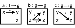
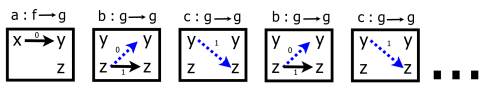
Three size-change graphs, which will provide a running example for this paper, are presented in Figure 3. The represented problem is size-change terminating. The call sequence is displayed in Figure 4, where a thread of infinite descent exists, starting in the second graph. This late-start thread proves the sequence terminating.
Every call sequence can be represented as a word in , and a SCT problem reduced to the containment of two -languages. The first language , contains all call sequences. The second language, some thread in has infinitely many 1-labeled arcs, contains only call sequences that guarantee termination. A SCT problem is size-change terminating if and only if .
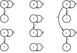
Lee et al. [24] describe two Büchi automata, and , that accept these languages. is simply the call graph of the program. waits in a copy of the call graph and nondeterministically chooses the beginning point of a descending thread. From there it ensures that a -labeled arc is taken infinitely often. To do so, it keeps two copies of each parameter, and transitions to the accepting copy only on a -labeled arc. Lee et al. prove that , and . The automata for our running example are provided in Figure 5.
222The original LJB construction [24] restricted starting
states in to functions. This was changed to simplify Section
3.4. The modification does not change the accepted
language.
{iteMize}
{iteMize}
Using the complementation constructions of either Section 2.1 or 2.2 and a lasso-finding algorithm, we can determine the containment of in . Lee et al. propose an alternative graph-theoretic algorithm, employing SCGs to encode descent information about entire call sequences. A notion of composition is used, where a call sequence has a thread from to if and only if the composition of the SCGs for each call, , contains the arc . The closure of under the composition operation, called , is then searched for a counterexample describing an infinite call sequence with no infinitely descending thread.
Let and be two SCGs. Their composition is defined as where:
Using composition, we can focus on a subset of graphs. Say that a graph is idempotent when . Each idempotent graph describes a cycle in the call graph, and a Ramsey-based argument shows that each cycle in the call graph can be accounted for by at least one idempotent graph. The composition of two graphs is shown in Figure 6, which describes the call sequence in Figure 4.
Algorithm LJB searches for a counterexample to size-change termination. First, it iteratively build the closure set : initialize as ; and for every and in , include the composition in . Second, the algorithm check every to ensure that if is idempotent, then has an associated thread with infinitely many 1-labeled arcs. This thread is represented by an arc of the form . There are pathological SCT problems for which the complexity of Algorithm LJB is .
The next theorem, whose proof uses a Ramsey-based argument, demonstrates the correctness of Algorithm LJB in determining the size-change termination of an SCT problem .
Theorem 2.2.
[24] A SCT problem is not size-change terminating iff , the closure of under composition, contains an idempotent SCG graph that does not contain an arc of the form .
3. Size-Change Termination and Ramsey-Based Containment
The Ramsey-based test of Section 2.1 and the LJB algorithm of Section 2.3 bear a remarkable similarity. In this section we bridge the gap between the Ramsey-based universality test and the LJB algorithm, by demonstrating that the LJB algorithm is a specialized realization of the Ramsey-based containment test. This first requires developing a Ramsey-based framework for Büchi containment testing.
3.1. Ramsey-Based Containment with Supergraphs
To test the containment of a Büchi automaton in a Büchi automaton , we could construct the complement of using either the Ramsey-based or rank-based construction, compute the intersection automaton of and , and search this intersection automaton for a lasso. With universality, however, we avoided directly constructing by exploiting the structure of states in the Ramsey-based construction (see Lemma 4). We demonstrate a similar test for containment.
Consider two automata, and . When testing the universality of , any word not in is a sufficient counterexample. To test we must restrict our search to the subset of accepted by . In Section 2.1, we defined a set of 0-1 arc-labeled graphs, whose elements provide a family of -languages that covers (see Lemma 2). We now define a set, , which provides a family of -languages covering .
We first define to capture the connectivity in . An element is a single arc asserting the existence of a path in from to . With each arc we associate a language, .
Given , say that iff there is a path in from to over .
Define as . The elements of , called supergraphs, are pairs consisting of an arc from and a graph from . Each element simultaneously captures all paths in and a single path in . The language is then . For convenience, we implicitly take , and say when . Since the language of each graph consists of finite words, we employ the concatenation of languages to characterize infinite runs. To do so, we first prove Lemma 6, which simplifies the concatenation of entire languages by demonstrating an equivalence to the concatenation of arbitrary words from these languages.
Lemma 6.
If , and , then
Proof 3.1.
Assume we have such an and . We demonstrate every word must be in . If we expand the premise, we obtain . This implies must be in and in . Next, we know that and . Thus by Lemma 1, , and . Along with the premise , we can now conclude , which is .
The languages , cover all finite subwords of . A subword of has at least one path between two states in , and thus is in the language of an arc in . Furthermore, by Lemma 1 this word is described by some graph, and the pair of the arc and the graph makes a supergraph. Unlike the case of graphs and , the languages of supergraphs do not form a partition of : a word might have multiple paths between states in , and so be described by more than one arc in . With them we construct the finite family of -languages that cover . Given , let be the -language . In analogy to Section 2.1, call proper if: (1) is non-empty; (2) and where and ; (3) and . Call a pair of supergraphs proper if is proper. We note that is non-empty if and are non-empty, and that, by the second condition, every proper is contained in .
Lemma 7.
Let and be two Büchi automata, and the corresponding set of supergraphs. .
Proof 3.2.
We extend the Ramsey argument of Lemma 2 to supergraphs.
Consider an infinite word with an accepting run in . As is accepting, we know that and for infinitely many . Since is finite, at least one accepting state must appear infinitely often. Let be the set of indexes such that .
We pause to observe that, by the definition of the languages of arcs, for every the word is in , and for every , , the word . Every language where and thus satisfies the second requirement of properness.
In addition to restricting our attention the subset of nodes where , we further partition into sets based on the prefix of until that point, where there is a associated with each possible graph . By Lemma 1, every finite word is in the language of some graph . Say that iff . As is finite, for some must be infinite. Let .
Similarly, by Lemma 1 we can use the word to define a partition of all unordered pairs of elements from . This partition consists of sets , such that iff . Without loss of generality, for , assume . Ramsey’s Theorem tells us that, given such a partition, there exists an infinite subset of and a such that for all pairs of distinct elements .
This is precisely to say there is a graph so that, for every , it holds that . thus partitions the word into
such that and for . Let and let . By the above partition of , we know that .
We now show that is proper. First, as , we know is non-empty. Second, as noted above, the second requirement is satisfied by the arcs and . Finally, we demonstrate the third condition holds. As for every , we have that . Both and are in and so . By the definition of the language of arcs, . Thus by Lemma 6, we can conclude that . Next observe that as for every pair , we have that . As are both in , it holds that . By the definition of the language of arcs, . By Lemma 6 we can now conclude . Therefore is a proper language containing .
Lemma 8.
Let and be two Büchi automata, and the corresponding set of supergraphs.
-
(1)
For all proper , either or .
-
(2)
iff every proper language .
-
(3)
Let be two supergraphs such that is proper. iff there exists such that and .
Proof 3.3.
Given two supergraphs and , recall that is the -language . Further note that and , and therefore .
In an analogous fashion to Section 2.1, we can use supergraphs to test the containment of two automata, and . Search all pairs of supergraphs, for a pair that is both proper and for which there does not exist a , such that and . Such a pair is a counterexample to containment. If no such pair exists, then .
3.2. Composition of Supergraphs
Employing supergraphs to test containment faces difficulty on two fronts. First, the number of supergraphs is very large. Second, verifying properness requires checking language nonemptiness and containment: PSPACE-hard problems. To address these problems we construct only supergraphs with non-empty languages. Borrowing the notion of composition from Section 2.3 allows us to use exponential space to compute exactly the needed supergraphs. Along the way we develop a polynomial-time test for the containment of supergraph languages. Our plan is to start with graphs corresponding to single letters and compose them until we reach closure. The resulting subset of , written , contains exactly the supergraphs with non-empty languages. In addition to removing the need to check for emptiness, composition allows us to test the sole remaining aspect of properness, language containment, in time polynomial in the size of the supergraphs. We begin by defining the composition of simple graphs.
Given two graphs and define their composition, written as , as the graph
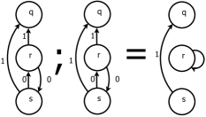
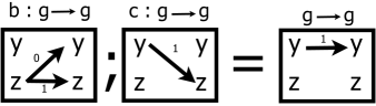
Figure 7 shows the composition of a simple graph with itself. Figure 2 is also illustrative, as the third graph is the composition of the first two.
We can then define the composition of two supergraphs and , written , as the supergraph . To generate exactly the set of supergraphs with non-empty languages, we start with supergraphs describing single letters. For a containment problem , define the subset of corresponding to single letters to be . For completeness, we present a constructive definition of .
We then define to be the closure of under
composition. Algorithm
DoubleGraphSearch, which we prove correct below, employs composition to check the
containment of two automata. It first generates the set of initial supergraphs, and then computes
the closure of this set under composition. Along the way it tests properness by using composition.
Every time it encounters a proper pair of supergraphs, it either verifies that a satisfying pair
of arcs exist, or halts with a counterexample to containment. We call this search the
double-graph search.
To begin proving our algorithm correct, we link composition and the concatenation of languages, first for simple graphs and then for supergraphs.
Lemma 9.
For every two graphs and , it holds that .
Proof 3.4.
Consider two words . By Definition 2.1, to prove we must show that for every : both (1) iff there is a path from to over , and (2) that iff there is an accepting path.
If an arc exists, then there is an such that and . By Definition 2.1, this implies the existence of a path from to over , and a path from to over . Thus is a path from to over .
If is , then either or must be 1. By Definition 2.1, (resp., ) is 1 iff there is an accepting path (resp., ) over (resp.,) from to (resp., to ). In this case (resp., ) is an accepting path in from to over .
Symmetrically, if there is a path from to over , then after reading we are in some state and have split into , so that is a path from to and a path from to . Thus by Definition 2.1 , , and .
Furthermore, if there is an accepting path from to over , then after reading we are in some state and have split the path into , so that is a path from to , and a path from to . Either or must be accepting, and thus by Definition 2.1 , , and either or must be . Therefore must be .
Lemma 10.
Let be supergraphs in such that , , and . Then iff .
Proof 3.5.
Assume as a premise. This implies . If either or are empty, then is empty and this direction holds trivially. Otherwise, take two words . By construction, and . The definition of the languages of arcs therefore implies the existence of a path from to over and a path from to over . Thus . Similarly, , and Lemma 9 implies that . Thus is in . and by Lemma 6 .
In the other direction, if , we show that . By definition, is . As , they are the composition of a finite number of graphs from . The above direction then demonstrates that they are non-empty, and there is a word . This expands to , which implies . By Lemma 9, is then in . Since, by Lemma 1, is the language of exactly one graph, we have that , which proves .
Lemma 10 provides the polynomial time test for properness employed in Algorithm DoubleGraphSearch. Namely, given two supergraphs and from , the pair is proper exactly when , , and . We now provide the final piece of our puzzle: proving that the closure of under composition contains every non-empty supergraph.
Lemma 11.
For two Büchi automata and , every , where , is in .
Proof 3.6.
Let where . Then there is at least one word, which is to say . By the definition of the languages of arcs, there is a path in over such that and .
We can now show the correctness of Algorithm DoubleGraphSearch, using Lemma 10 to justify testing properness with composition, and Lemma 12 below to justify the correctness and completeness of our search for a counterexample.
Lemma 12.
Let and be two Büchi automata. is not contained in iff contains a pair of supergraphs , such that is proper and there do not exist arcs and , .
Proof 3.7.
Theorem 3.8.
For every two Büchi automata and , it holds that iff DoubleGraphSearch(,) returns Contained.
Proof 3.9.
By Lemma 10, testing for composition is equivalent to testing for language containment, and the outer conditional in Algorithm DoubleGraphSearch holds only for proper pairs of supergraphs. By Lemma 12, the inner conditional checks if a proper pair of supergraphs is a counterexample, and if no such proper pair in is a a counterexample then containment must hold.
3.3. Strongly Suffix Closed Languages
Algorithm DoubleGraphSearch has much the same structure as Algorithm LJB. The most noticeable difference is that Algorithm DoubleGraphSearch checks pairs of supergraphs, where Algorithm LJB checks only single size-change graphs. Indeed, Theorem 2.2 suggests that, for some languages, a cycle implies the existence of a lasso. When proving containment of Büchi automata with such languages, it is sufficient to search for a graph , where , with no arc . This single-graph search reduces the complexity of our algorithm significantly. What enables this in size-change termination is the late-start property: threads can begin at arbitrary points. We here define the class of automata amenable to this optimization, first presenting the case for universality testing, without proof, for clarity.
In size-change termination, the late-start property asserts that an accepting cycle can start at an arbitrary point. Intuitively, this suggests that an arc might not need a matching prefix in some : the cycle can just start at . In the context of universality, we can apply this method when it is safe to add or remove arbitrary prefixes of a word. To describe these languages we extend the standard notion of suffix closure. A language is suffix closed when, for every , every suffix of is in .
A language is strongly suffix closed if it is suffix closed and for every , we have that .
Lemma 13.
Let be an Büchi automaton where every state in is reachable and is strongly suffix closed. is not universal iff the set of supergraphs with non-empty languages, , contains a graph such that and does not contain an arc of the form .
As an intuition for the correctness of Lemma 13, note that the existence of an 1-labeled cyclic arc in implies a loop, that being reachable implies a prefix can be prepended to this loop to make a lasso, and that strong suffix closure allows us to swap this prefix for the prefix of every other word that share this cycle.
To extend this notion to handle containment questions , we restrict our focus to words in . Instead of requiring to be closed under arbitrary prefixes, need only be closed under prefixes that keep the word in .
A language is strongly suffix closed with respect to when is suffix closed and, for every , if then .
When checking the containment of in for the case when is strongly suffix closed with respect to , we can employ a the simplified algorithm below. As in Algorithm DoubleGraphSearch, we search all supergraphs in . Rather than searching for a proper pair of supergraphs, however, Algorithm SingleGraphSearch searches for a single supergraph where that does not contain an arc of the form . We call this search the single-graph search.
We now prove Algorithm SingleGraphSearch correct. Theorem 3.10 demonstrates that, under the requirements specified, the presence of a single-graph counterexample refutes containment, and the absence of such a supergraph proves containment.
Theorem 3.10.
Let and be two Büchi automata where , every state in is reachable, and is strongly suffix closed with respect to . Then is not contained in iff contains a supergraph such that , , and does not contain an arc .
Proof 3.11.
In one direction, assume contains a supergraph where , , and there is no arc . We show that is a proper language not contained in . As , we know is not empty, implying is non-empty. As , it holds that . By Lemma 10, the premise implies , and is proper. Finally, as there is no , by Theorem 3.8, , and is a counterexample to .
In the opposite direction, assume the premise that does not contain a supergraph where , , and there is no arc . We prove that every word is also in . Take a word . By Lemma 7, is in some proper language and can be broken into where .
Because is proper, Lemma 10 implies where and . This, along with our premise, implies contains an arc . Since all states in are reachable, there is and with a path in from to over . By Lemma 4, this implies is accepted by . For to strongly suffix closed with respect to , it must be suffix closed. Therefore . Now we move to , and note that the premise implies is suffix closed. Thus the fact that implies . Since is strongly suffix closed with respect to , and , it must be that .
3.4. From Ramsey-Based Containment to Size-Change Termination
We now delve into the connection between the LJB algorithm for size-change termination and the single-graph search algorithm for Büchi containment. We will show that Algorithm LJB is a specialized realization of Algorithm SingleGraphSearch. Given an SCT problem , size-change graphs in LJB() are direct analogues of supergraphs in SingleGraphSearch(, ). For convenience, take , , and .
We first show that and satisfy the preconditions of Algorithm SingleGraphSearch: that ; that every state in is reachable; and that is strongly suffix closed with respect to . For the first and second requirement, it suffices to observe that every state in both and is initial.333In the original reduction, 1-labeled parameters may not have been reachable.
For the third, strong suffix closure is a direct consequence of the definition of a thread: since a thread can start at arbitrary points, it does not matter what call path we use to reach that point. Adding a prefix to a call path cannot cause that call path to become non-terminating. Thus the late-start property is precisely being strongly suffix closed with respect to , and we can employ the single-graph search.
Consider supergraphs in , from here simply denoted by . The state space of is the set of functions , and the state space of is the union of and , the set of all -labeled parameters. A supergraph in thus comprises an arc in and a -labeled graph over . The arc asserts the existence of a call path from to , and the graph captures the relevant information about corresponding paths in .
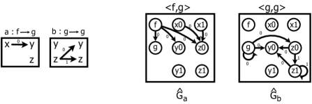
These supergraphs are almost the same as SCGs, (See Figure 8). Aside from notational differences, both contain an arc asserting the existence of a call path between two functions, and a -labeled graph. There are nodes in both graphs that correspond to parameters of functions, and arcs between two such nodes describe a thread between the corresponding parameters. The analogy falls short, however, on three points:
-
(1)
In SCGs, nodes are always parameters of functions. In supergraphs, nodes can be either parameters of functions or function names.
-
(2)
In SCGs, nodes are unlabeled. In supergraphs, nodes are labeled either or .
-
(3)
In an SCG, only the nodes corresponding to the parameters of two specific functions are present. In a supergraph, nodes corresponding to every parameter of every function exist.
Each difference is an opportunity to specialize the Ramsey-based containment algorithm, Algorithm SingleGraphSearch, by simplifying supergraphs. When these specializations are taken together, we have Algorithm LJB.
-
1
No functions in are accepting for , and once we transition out of into we can never return to . Therefore nodes corresponding to function names can never be part of a descending arc . Since we only search for arcs of the form , we can simplify supergraphs in by removing all nodes corresponding to functions.
-
2
The labels on parameters are the result of encoding a Büchi edge acceptance condition in a Büchi state acceptance condition automaton, and can be dropped from supergraphs with no loss of information. Consider an arc . If is 1, we know the corresponding thread contains a descending arc. The value of tells us if the final arc in the thread is descending, but which arc is descending is irrelevant. Thus it is safe to simplify supergraphs in by removing labels on parameters.
-
3
While all parameters have corresponding states in , each supergraph describes threads in a call sequence between two particular functions. There are no threads in this call sequence between parameters of other functions, and so no supergraph with a non-empty language has arcs between the parameters of other functions. We can thus simplify supergraphs in by removing all nodes corresponding to parameters of other functions.
To formalize this notion of simplification, we first define, , the set of simplified supergraphs and show that is in one-to-one correspondence with , the closure of under composition.
Say that simplifies to when iff there exists such that . Let be , and be the closure of under composition.
We can map SCGs directly to elements of . Say when iff . Note that the composition operations for supergraphs of this form is identical to the composition of SCGs: if and , then . Therefore every element of simplifies to some element of .
We now show that supergraphs whose languages contain single characters are in one-to-one correspondence with , and that every idempotent element of contains an arc of the form exactly when the closure of under composition does not contain a counterexample graph.
Lemma 14.
Let be an SCT problem.
-
(1)
The relation is a one-to-one correspondence between and
-
(2)
is not size-change terminating iff contains a supergraph such that and there does not exist an arc of the form in .
Proof 3.12.
(1): Given a size-change graph , we construct a unique supergraph such that . Every size-change graph is the SCG for a call site from to . This is a call sequence of length one. Thus there is a so that and . We show that the simplification of is equivalent to . By the reduction of Definition 2.3 and the definition of graphs in Definition 2.1, the arc , for some , exactly when . The supergraph simplifies to some . By the definition of simplification, exactly when . Thus .
In the other direction, iff there exists a that simplifies to . By Definition 3.2, which defines and Definition 2.3, exists because there is a call site . This call site corresponds to a SCG . Analogously to the above, by Definition 2.3 the arcs in between parameters correspond to arcs in : , for some , exactly when . These are the only arcs that remain after simplification, during which the labels are removed. Thus .
(2): By (1), is in one-to-one correspondence with under the relation. Since composition of supergraphs and SCGs is identical, , the closure of under composition, is in one-to-one correspondence with the . Claim (2) then follows from Theorem 2.2 and claim (1).
In conclusion, we can specialize the Ramsey-based containment algorithm for in two ways. First, by Theorem 3.10 we know that if and only if contains an idempotent graph with no arc of the form . Thus we can employ the single-graph search instead of the double-graph search. Secondly, we can simplify supergraphs in by removing the labels on nodes and keeping only nodes associated with appropriate parameters for the source and target function. The simplifications of supergraphs whose languages contain single characters are in one-to-one corresponding with , the initial set of SCGs. As every state in is accepting, every idempotent supergraph can serve as a counterexample. Therefore if and only if the closure of the set of simplified supergraphs, which is in one-to-one correspondence with , under composition does not contain an idempotent supergraph with no arc of the form . This is precisely Algorithm LJB.
4. Empirical Analysis
All the Ramsey-based algorithms presented in Section 2.3 have worst-case running times that are exponentially larger than those of the rank-based algorithms. We now compare existing, Ramsey-based, SCT tools tools to a rank-based Büchi containment solver on the domain of SCT problems. To facilitate a fair comparison, we briefly describe two improvements to the algorithms presented above.
4.1. Towards an Empirical Comparison
First, in constructing the analogy between SCGs in the LJB algorithm and supergraphs in the Ramsey-based containment algorithm, we noticed that supergraphs contain nodes for every parameter, while SCGs contain only nodes corresponding to parameters of relevant functions. These nodes are states in . While we can specialize the Ramsey-based test to avoid them, Büchi containment solvers might suffer. These states duplicate information. As we already know which functions each supergraph corresponds to, there is no need for each node to be unique to a specific parameter.
These extra states emerge because only accepts strings that are contained in , and in doing so demands that parameters only be reached by appropriate call paths. But the behavior of on strings not in is irrelevant to the question of , and we can replace the names of parameters in with their location in the parameter list. Further, we can rely on to verify the sequence of function calls before our accepting thread and make do with a single waiting state. As an example, see Figure 9.
Given an SCT problem and a projection of all parameters onto their positions in the parameter list, define:
| where | ||||
Lemma 15.
iff
Proof 4.1.
The languages of and are not the same. What we demonstrate is that for every word in , we can convert an accepting run in one of or into an accepting run in the other. Recall that the states of are functions . States of are either elements of or elements of , the set of labeled parameters. For convenience, given a pair , define to be .
Consider an accepting run of over a word . Let be the sequence of states in such that when , , and when , . By the definition of , always transitions to and a transition between and implies a transition between and . Therefore is a run of over . Furthermore, if is an accepting state in , and is an accepting state . Thus, is an accepting run of over .
Conversely, consider a word with an accepting run of and an accepting run of . We define an accepting run of on . Each depends on the corresponding and . If and , then . If and , then where is the th parameter in ’s parameter list.
For a call , take two labeled parameters, a labeled parameter of and a labeled parameter of . If is a transition in , then is a transition in . Therefore is a run of on . Furthermore, note that and iff . Therefore is an accepting run.
Second, in [4], Ben-Amram and Lee present a polynomial approximation of the LJB algorithm for SCT. To facilitate a fair comparison, they optimize the LJB algorithm for SCT by using subsumption to remove certain SCGs when computing the closure under composition. This suggests that the single-graph search of Algorithm SingleGraphSearch can also employ subsumption. When computing the closure of a set of graphs under compositions, we can ignore elements when they are approximated by other elements. Intuitively, a graph approximates another graph when it is strictly harder to find a 1-labeled sequence of arcs through than through . If we can replace with without losing arcs, we do not have to consider . When the right arc can be found in , then it also occurs in . On the other hand, when does not have a satisfying arc, then we already have a counterexample.
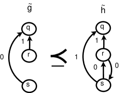
Formally, given two graphs say that approximates , written , when for every arc there is an arc , . An example is provided in Figure 10. Note that approximation is a transitive relation. In order to safely employ approximation as a subsumption relation, Ben-Amram and Lee replace the search for a single arc in idempotent graphs with a search for a strongly connected component in all graphs. This was proven to be safe in [13]: when computing the closure of under composition, it is sufficient to store only maximal elements under this relation.
4.2. Experimental Results
All experiments were performed on a Dell Optiplex GX620 with a single 1.7Ghz Intel Pentium 4 CPU and 512 MB. Each tool was given 3500 seconds, a little under one hour, to complete each task.
Tools: The formal-verification community has implemented rank-based tools in order to measure the scalability of various approaches. The programming-languages community has implemented several Ramsey-based SCT tools. We use the best-of-breed rank-based tool, Mh, developed by Doyen and Raskin [9], that leverages a subsumption relation on ranks. We expanded the Mh tool to handle Büchi containment problems with arbitrary languages, thus implementing the full containment-checking algorithm presented in their paper.
We use two Ramsey-based tools. SCTP is a direct implementation of the LJB algorithm of Theorem 2.2, written in Haskell [15]. We have extended SCTP to reduce SCT problems to Büchi containment problems, using either Definition 2.3 or 4.1. sct/scp is an optimized C implementation of the SCT algorithm, which uses the subsumption relation of Section 4.1 [4].
Problem Space: Existing experiments on the practicality of SCT solvers focus on examples extracted from the literature [4]. We combine examples from a variety of sources [1, 4, 15, 17, 24, 28, 32]. The time spent reducing SCT problems to Büchi automata never took longer than 0.1 seconds and was dominated by I/O. Thus this time was not counted. We compared the performance of the rank-based Mh solver on the derived Büchi containment problems to the performance of the existing SCT tools on the original SCT problems. If an SCT problem was solved in all incarnations and by all tools in less than 1 second, the problem was discarded as uninteresting. Unfortunately, of the 242 SCT problems derived from the literature, only 5 prove to be interesting.
Experiment Results: Table 1 compares the performance of the rank-based Mh solver against the performance of the existing SCT tools, displaying which problems each tool could solve, and the time taken to solve them. Of the interesting problems, both SCTP and Mh could only complete 3. On the other hand, sct/scp completed all of them, and had difficulty with only one problem.
| Problem | SCTP (s) | Mh (s) | sct/scp (s) |
|---|---|---|---|
| ex04 [4] | 1.58 | Time Out | 1.39 |
| ex05 [4] | Time Out | Time Out | 227.7 |
| ms [15] | Time Out | 0.1 | 0.02 |
| gexgcd [15] | 0.55 | 14.98 | 0.023 |
| graphcolour2 [17] | 0.017 | 3.18 | 0.014 |
The small problem space makes it difficult to draw firm conclusions, but it is clear that Ramsey-based tools are comparable to rank-based tools on SCT problems: the only tool able to solve all problems was Ramsey based. This is surprising given the significant difference in worst-case complexity, and motivates further exploration.
5. Reverse-Determinism
In the previous section, the theoretical gap in performance between Ramsey and rank-based solutions was not reflected in empirical analysis. Upon further investigation, it is revealed that a property of the domain of SCT problems is responsible. Almost all problems, and every difficult problem, in this experiment have SCGs whose nodes have an in-degree of at most 1. This property was first observed by Ben-Amram and Lee in their analysis of SCT complexity [4]. After showing how this property explains the performance of Ramsey-based algorithms, we explore why this property emerges and argue that it is a reasonable property for SCT problems to possess. Finally, we improve the rank-based algorithm for problems with this property.
As stated above, all interesting SCGs in this experiment have nodes with at most one incoming edge. In analogy to the corresponding property for automata, we call this property of SCGs reverse-determinism. Say that a SCG is reverse-deterministic if every parameter of has at most one incoming edge. Given a set of reverse-deterministic SCGs , we observe three consequences. First, a reverse-deterministic SCG can have no more than arcs: one entering each node. Second, there are only possible such combinations of arcs. Third, the composition of two reverse-deterministic SCGs is also reverse-deterministic. Therefore every element in the closure of under composition is also reverse-deterministic. These observations imply that the closure of under composition contains at most SCGs. This reduces the worst-case complexity of the LJB algorithm to . In the presence of this property, the massive gap between Ramsey-based algorithms and rank-based algorithms vanishes, helping to explain the surprising strength of the LJB algorithm.
Lemma 16.
When operating on reverse-deterministic SCT problems, the LJB algorithm has a worst-case complexity of .
Proof 5.1.
A reverse-deterministic SCT problem contains only reverse-deterministic SCGs. Observe that the composition of two reverse-deterministic SCGs is itself reverse-deterministic. As there are only possible reverse-deterministic SCGs, the closure computed in the LJB algorithm cannot become larger than . The LJB algorithm checks each graph in the closure exactly once, and so has a time complexity of .
It is not a coincidence that all SCT problems considered possess this property. As noted in [4], straightforward analysis of functional programs generates only reverse-deterministic problems. In fact, every tool we examined is only capable of producing reverse-deterministic SCT problems. To illuminate the reason for this, imagine a SCG where has two parameters, and , and the single parameter . If is not reverse deterministic, this implies both and have arcs, labeled with either 0 or 1, to . This would mean that ’s value is both always smaller than or equal to and always smaller than or equal to .
The program in Algorithm 4 can produce non-reverse-deterministic size-change graphs, and serves to demonstrate the difficult analysis required to do so444This example emerges from the Terminweb experiments by Mike Codish, and was translated into a functional language by Amir Ben-Amram and Chin Soon Lee. The authors are grateful to Amir Ben-Amram for bringing this illustrative example to our attention.. Consider the SCG for the call on line 4. It is clear there should be a -labeled arc from to . To reach this point, however, we must satisfy the inequality on line 4. Therefore we can also assert that , and include a -labeled arc from to . This is a kind of analysis is difficult to make, and none of the size-change analyzers we examined were capable of detecting this relation.
5.1. Reverse Determinism and Rank-Based Containment
Since the Ramsey-based approach benefited so strongly from reverse-determinism, we examine the rank-based approach to see if it can similarly benefit. As a first step, we demonstrate that reverse-deterministic automata have a maximum rank of 2, dramatically lowering the complexity of complementation to . We note, however, that given a reverse-deterministic SCT problem ,i the automaton is not reverse-deterministic. Thus a separate proof is provided to demonstrate that the rank of the resulting automata is still bounded by 2.
An automaton is reverse-deterministic when no state has two incoming arcs labeled with the same character. Formally, an automaton is reverse-deterministic when, for each state and character , there is at most one state such that . As a corollary to Lemma 16, the Ramsey-based complementation construction has a worst-case complexity of for reverse deterministic automata With reverse-deterministic automata, we do not have to worry about multiple paths to a state. As a consequence, a maximum rank of 2, rather than , suffices to prove termination of every path, and the worst-case bound of the rank-based construction improves to .
Theorem 5.2.
Given a reverse-deterministic Büchi automaton with states, there exists an automaton with states such that .
Proof 5.3.
In a run DAG of a reverse-deterministic automaton, all nodes have only one predecessor. This implies the run DAG is a tree, and that the number of infinite paths grows monotonically and at some point stabilizes. Call this point . If is rejecting, we demonstrate that there is a point past which all accepting states are finite in . Observe that each infinite path eventually stops visiting accepting states. Let be the last such point over all infinite paths, or , whichever is greater. Past , consider a branch off this path containing an accepting state. This branch cannot be a new infinite path, as the number of infinite paths is stable. This branch cannot lead to an existing infinite path, because that would violate reverse determinism. Therefore this path must be finite, and the accepting state is finite.
Recall that is , is with all finite nodes removed, is with all -free nodes removed, and is with all finite nodes removed. Because there are no infinite accepting nodes past , has no accepting nodes at all past . Thus every node past is -free in , and has no nodes past . Thus is empty, and the DAG has a rank of at most . We conclude that the maximum rank of rejecting run is 2, and the state space of the automaton in Definition 2.2 can be restricted to level rankings with no ranking larger than 2.
Unfortunately, neither the reduction of Definition 2.3 nor the reduction of Definition 4.1 preserve reverse determinism, which is to say that given a reverse-deterministic SCT problem, they do not produce a reverse-deterministic Büchi containment problem. However, we can show that, given a reverse-deterministic SCT problem, the automata produced by Definition 4.1 does have a maximum rank of 2. A similar claim could be made about Definition 2.3 with minor adjustments.
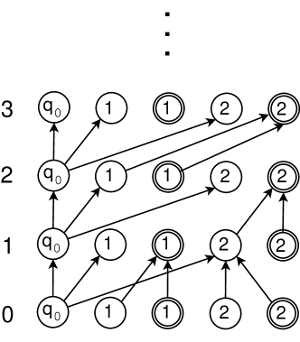
Formally, we prove that for every reverse-deterministic SCT problem , has a maximum rank of 2. Let be an infinite word not in , and the rejecting run DAG of on . There are two kinds of states in . There is a waiting state, , which always transitions to itself, and there are two states for every variable position , and . Every state is an initial state. Consider , the run DAG of on a word . Each character represents a function call from some function to another function . At level of the run DAG, the waiting state has outgoing edges to itself and the positions of 0-labeled parameters of . Each variable state only has outgoing edges to a 0 or 1-labeled position. To get an idea of what the run DAG looks like, Figure 11 displays a supergraph of the run DAG that includes all states at all levels, even if they are not reachable.
We now prove that the rejecting run DAG has a maximum rank of 2. To do so, we analyze the structure of by first examining subgraphs, and then extending these observations to . Let be the subgraph of the run DAG that omits the waiting state at every level of the run DAG. Every path in corresponds to a (possibly finite) thread in the call sequence .
Lemma 17.
For a level , , and , at most one of and has incoming edges in .
Proof 5.4.
For , this holds trivially. For , take a pair of nodes and . The edges from level correspond to transitions in on some call . As is a call to a single function, we know there is a unique variable such that . Because is reverse deterministic, we know that there is at most one edge in leading to . If there is no edge, then there are no edges entering or .
Otherwise there is exactly one edge in , , . In this case, the only nodes in level with an edge to either or are and . By the transition function , both of these states transition only to , and only has incoming edges in .
Now, define to be the subgraph of containing only nodes with an incoming edge in . This removes nodes whose only incoming edge was from . While this excludes nodes that begin threads, this cannot change the accepting or rejecting nature of a thread.
Lemma 18.
-
(1)
is a forest.
-
(2)
Every infinite path in appears in .
-
(3)
Every accepting node in is also in .
Proof 5.5.
(1): Lemma 17 implies, for every and , that only one of and
is in . Combined with the fact that is
reverse deterministic, every node in can have at most one incoming
edge, and thus it is a forest.
(2): For every infinite path in , all nodes past the first have an
incoming edge from . Every node with an incoming edge from is in
. Thus for every infinite path in , a corresponding path, perhaps
without the first node, occurs in .
(3): Only nodes of the form are accepting. Let
be a accepting node. By the definition of a run DAG, must be
reachable if it is in . Thus there is an edge from another node in
to . By the transition function , the waiting state
only has an edge to . Therefore the only nodes that have an edge
to are nodes of the form . All nodes of this
form are in , and therefore has an incoming edge from
, and is in .
We can now make observations about the rejecting run DAGs of that mirror those made about rejecting run DAGs of reverse deterministic automata.
Lemma 19.
There exists where for all , has no infinite accepting nodes at level .
Proof 5.6.
As is a forest, the number of infinite nodes in level cannot be smaller than the number of infinite nodes in level . Thus at some level the number of infinite nodes reaches a maximum. Past level , each infinite node has a unique infinite path through . As is rejecting, every infinite path eventually stops visiting accepting nodes at some level. Let be the last such point over all infinite paths, or , whichever is greater. Past , consider an accepting node that branch off an infinite path. This branch cannot be part of the existing infinite path, as this path has ceased visiting accepting nodes. Likewise, this branch cannot be part of a new infinite path, as the number of infinite paths can not increase. Therefore must be finite.
Lemma 20.
is empty.
Proof 5.7.
Let be the level past which there are no infinite accepting nodes in , as per Lemma 19. This precisely means that, past , every accepting node in has a finite path. As all accepting nodes in are in , past every reachable accepting node in has a finite path. After level , contains only non-accepting nodes. This implies that contains no nodes past , and therefore that is empty.
Theorem 5.8.
Given a reverse-deterministic SCT problem with maximum arity , there is an automaton with at most states such that .
5.2. Experiments revisited
In light of this discovery, we revisit the experiments and again compare rank and Ramsey-based approaches on SCT problems. This time we tell Mh, the rank-based solver, that the problems have a maximum rank of 2. Table 2 compares the running time of Mh and sct/scp on the five most difficult problems. As before, time taken to reduce SCT problems to automata containment problems was not counted.
| Problem | Mh (s) | sct/scp (s) |
|---|---|---|
| ex04 | 0.01 | 1.39 |
| ex05 | 0.13 | 227.7 |
| ms | 0.1 | 0.02 |
| gexgcd | 0.39 | 0.023 |
| graphcolour2 | 0.044 | 0.014 |
While our problem space is small, the theoretical worst-case bounds of Ramsey and rank-based approach appears to be reflected in the table. The Ramsey-based sct/scp completes some problems more quickly, but in the worst cases of ex04 and ex05, sct/scp performs significantly more slowly than Mh. It is worth noting, however, that the benefits of reverse-determinism on Ramsey-based approaches emerges automatically, while rank-based approaches must explicitly test for this property in order to exploit it.
5.3. Monotonicity Constraints: Termination Problems Lacking Reverse-Determinism
Monotonicity constraints [8] are a generalization of size-change graphs. While an SCG for a call from to is bipartite, with edges only from variables of to variables of , monotonicity constraints allow edges between any two variables, even of the same function. In addition, while SCGs only have edges representing less than and less than or equal relations, monotonicity constraints allow edges representing equality relations. A collection of monotonicity constraints is called a monotonicity constraint system (MCS). For a formal presentation, please see [3].
Deciding termination for MCS problems is more involved than for SCT problems, but correctness similarly relies on Ramsey’s Theorem [8]. One method is to reduce a MCS to an SCT problem through elaboration [3]. Unfortunately, elaboration is an exponential reduction, and increases the size of the MCS. Alternatively, it is possible to project an individual monotonicity constraint into an SCG in a lossy fashion. To do so, simply remove all edges that are not from a variable of to a variable of , and replace equality edges with less-than-or-equal edges. By projecting every monotonicity constraint in an MCS down to a SCG, we obtain a SCT problem. Doing so, however, often removes valuable information that can still be encoded in a size-change graph. To preserve this information, new arcs that are logically implied by existing arcs can be added to the monotonicity constraint before the constraint is projected to a SCG. The simplest implied arcs are those derived from equality edges: given two arcs and , add to the monotonicity constraint. Similarly, given an arc , add . More complex implied arcs can be computed by similarly composing other arcs.
We obtained a corpus of 373 monotonicity constraint systems from [7]. In each case, we produced three SCT problems from each MCS: one from directly projecting, one by computing arcs implied by equality before projecting, and one by computing all implied arcs before projecting. We again defined a problem to be interesting if either sct/scp or Mh took more than 1 second to solve the problem. For every interesting problem, there was no difference in result and no significant difference in running time between the two types of implied arcs. Thus we consider only the third, most complex, SCT problem generated from each MC problem, resulting in nine final problems.
None of the interesting SCT problem produced in this fashion were reverse deterministic. Given the complexity of monotonicity constraints, this is perhaps unsurprising. Four of the resulting problems were non-terminating. For these problems, the maximum rank can be computed. To do so, Mh is initially limited to a rank of 1, and the rank is increased until Mh can detect non-termination. Table 3 displays the results for these problems. Despite the lack of reverse-determinism, none of these problems proved difficult for sct/scp: consuming at most 0.4 seconds. However, several were difficult for Mh, including one that took over eight minutes. In cases where we could bound the rank, the running time for Mh often improved dramatically. While we again have only a sparse corpus of interesting problems, these results serve to emphasize the importance of reverse determinism. Perhaps more interestingly, they suggest that, even in cases where reverse determinism does not hold, the Ramsey-based approach performs well.
| Problem | rank | Mh (s) | sct/scp (s) |
|---|---|---|---|
| Test3 | N/A | 4.44 | 0.047 |
| Test4 | N/A | 4.65 | 0.079 |
| Test5 | N/A | 111.8 | 0.074 |
| Test6 | N/A | 482.0 | 0.097 |
| WorkingSignals | 13 | 1.32 (1.0) | 0.098 |
| Gauss | 3 | 1.10 (0.08) | 0.146 |
| PartitionList | 3 | 1.38 (0.22) | 0.081 |
| Sudoku | 5 | 7.18 (2.42) | 0.405 |
6. Conclusion
In this paper we demonstrate that the Ramsey-based size-change termination algorithm proposed by Lee, Jones, and Ben-Amram [24] is a specialized realization of the 1987 Ramsey-based complementation construction [5, 29]. With this link established, we compare rank-based and Ramsey-based tools on the domain of SCT problems. Initial experimentation revealed a surprising competitiveness of the Ramsey-based tools, and led us to further investigation. We discover that SCT problems are naturally reverse-deterministic, reducing the complexity of the Ramsey-based approach. By exploiting reverse determinism, we were able to demonstrate the superiority of the rank-based approach.
Our initial test space of SCT problems was unfortunately small, with only five interesting problems emerging. Despite the very sparse space of problem, they still yielded two interesting observations. First, subsumption appears to be critical to the performance of Büchi complementation tools using both rank and Ramsey-based algorithms. It has already been established that rank-based tools benefit strongly from the use of subsumption [9]. Our results demonstrate that Ramsey-based tools also benefit from subsumption, and in fact experiments with removing subsumption from sct/scp seem to limit its scalability. Second, by exploiting reverse determinism, we can dramatically improve the performance of both rank and Ramsey-based approaches to containment checking.
Reverse determinism, however, is not the whole story in comparing the rank and Ramsey based approaches. On a separate corpus of problems derived from Monotonicity Constraints, which are not reverse-deterministic, the Ramsey-based approach outperformed the rank-based approach in every interesting case. It should be noted that, in addition to reverse determinism, there are several ways to achieve a better bound on the maximum rank than [16, 18], even for problems that are not known to be non-terminating. The rank-based approach might prove more competitive if such analyses were applied before checking containment. None the less, it is clear that despite the theoretical differences in complexity, we cannot discount the Ramsey-based approach. The competitive performance of Ramsey-based solutions remains intriguing.
In [9, 30], a space of random automata universality problems is used to provide a diverse problem domain. Unfortunately, it is far more complex to similarly generate a space of random SCT problems. First, universality involves a single automaton: SCT problems check the containment of two automata, with a corresponding increase in parameters. Worse, there is no reason to expect that one random automaton will have any probability of containing another random automaton. Sampling this problem space is further complicated by the low transition density of reverse-deterministic problems: in [9, 30] the most interesting problems had a transition density of 2.
On the theoretical side, we have extended the subsumption relation present in sct/scp. Recent work has extended the subsumption relation to the double-graph search of Algorithm DoubleGraphSearch, and others have improved the relation through the use of simulation [2, 14]. Doing so has enabled us to compared Ramsey and rank-based approaches on the domain of random universality problems [14], with promising results. Future work will investigate how to generate an interesting space of random containment problems, addressing the concerns raised above.
The effects of reverse-determinism on the complementation of automata bear further study. Reverse-determinism is not an obscure property, it is known that automata derived from LTL formula are often reverse-deterministic [12]. As noted above, both rank and Ramsey-based approaches improves exponentially when operating on reverse-deterministic automata. Further, Ben-Amram and Lee have defined SCP, a polynomial-time approximation algorithm for SCT [4]. For a wide subset of SCT problems with restricted in degrees, including the set used in this paper, SCP is exact. In terms of automata, this property is similar, although perhaps not identical, to reverse-determinism. The presence of an exact polynomial algorithm for the SCT case suggests a interesting subset of Büchi containment problems may be solvable in polynomial time. The first step in this direction would be to determine what properties a containment problem must have to be solved in this fashion.
References
- [1] Daedalus. Available on: http://www.di.ens.fr/~cousot/projects/DAEDALUS/index.shtml.
- [2] P.A. Abdulla, Y.-F. Chen, L. Holík, R. Mayr, and T. Vojnar. When simulation meets antichains. In Tools and Algorithms for the Construction and Analysis of Systems, volume 6015 of Lecture Notes in Computer Science, pages 158–174. Springer, 2010.
- [3] A.M. Ben-Amram. Size-change termination, monotonicity constraints and ranking functions. Logical Methods in Computer Science, 6(3), 2010.
- [4] A.M. Ben-Amram and C.S. Lee. Program termination analysis in polynomial time. ACM Trans. Program. Lang. Syst., 29:5:1–5:37, January 2007.
- [5] J.R. Büchi. On a decision method in restricted second order arithmetic. In Proc. Int. Congress on Logic, Method, and Philosophy of Science. 1960, pages 1–12. Stanford University Press, 1962.
- [6] Y. Choueka. Theories of automata on -tapes: A simplified approach. Journal of Computer and Systems Science, 8:117–141, 1974.
- [7] M. Codish, I. Gonopolskiy, A.M. Ben-Amram, C. Fuhs, and J. Giesl. SAT-based termination analysis using monotonicity constraints over the integers. Theory and Practice of Logic Programming, 26th Int’l. Conference on Logic Programming (ICLP’11) Special Issue, 11:503–520, July 2011.
- [8] M. Codish, V. Lagoon, and P.J. Stuckey. Testing for termination with monotonicity constraints. In Twenty First International Conference on Logic Programming, volume 3668 of Lecture Notes in Computer Science, pages 326–340. Springer-Verlag, October 2005.
- [9] L. Doyen and J.-F. Raskin. Improved algorithms for the automata-based approach to model-checking. In Tools and Algorithms for the Construction and Analysis of Systems, volume 4424 of Lecture Notes in Computer Science, pages 451–465. Springer, 2007.
- [10] L. Doyen and J.-F. Raskin. Antichains for the automata-based approach to model-checking. Logical Methods in Computer Science, 5(1), 2009.
- [11] E.A. Emerson and C.-L. Lei. Efficient model checking in fragments of the propositional -calculus. In Proc. 1st IEEE Symp. on Logic in Computer Science, pages 267–278, 1986.
- [12] E.A. Emerson and A.P. Sistla. Deciding full branching time logics. Information and Control, 61(3):175–201, 1984.
- [13] S. Fogarty. Büchi containment and size-change termination. Master’s thesis, Rice University, 2008.
- [14] S. Fogarty and M.Y. Vardi. Efficient Büchi universality checking. In Tools and Algorithms for the Construction and Analysis of Systems, volume 6015 of Lecture Notes in Computer Science, pages 205–220. Springer, 2010.
- [15] C.C. Frederiksen. A simple implementation of the size-change termination principle. Available at: ftp://ftp.diku.dk/diku/semantics/papers/D-442.ps.gz, 2001.
- [16] E. Friedgut, O. Kupferman, and M.Y. Vardi. Büchi complementation made tighter. In 2nd Int. Symp. on Automated Technology for Verification and Analysis, volume 3299 of Lecture Notes in Computer Science, pages 64–78. Springer, 2004.
- [17] Arne J. Glenstrup. Terminator II: Stopping partial evaluation of fully recursive programs. Master’s thesis, DIKU, University of Copenhagen, June 1999.
- [18] S. Gurumurthy, O. Kupferman, F. Somenzi, and M.Y. Vardi. On complementing nondeterministic Büchi automata. In Proc. 12th Conf. on Correct Hardware Design and Verification Methods, volume 2860 of Lecture Notes in Computer Science, pages 96–110. Springer, 2003.
- [19] N.D Jones and Nina Bohr. Termination analysis of the untyped -calculus. In Rewriting Techniques and Applications. Proceedings, volume 3091 of Lecture Notes in Computer Science, pages 1–23. Springer, 2004.
- [20] N. Klarlund. Progress Measures and finite arguments for infinite computations. PhD thesis, Cornell University, 1990.
- [21] O. Kupferman and M.Y. Vardi. Weak alternating automata are not that weak. In Proc. 5th Israeli Symp. on Theory of Computing and Systems, pages 147–158. IEEE Computer Society Press, 1997.
- [22] O. Kupferman and M.Y. Vardi. Synthesizing distributed systems. In Proc. 16th IEEE Symp. on Logic in Computer Science, pages 389–398, 2001.
- [23] O. Kupferman and M.Y. Vardi. Weak alternating automata are not that weak. ACM Transactions on Computational Logic, 2(2):408–429, 2001.
- [24] C.S. Lee, N.D. Jones, and A.M. Ben-Amram. The size-change principle for program termination. In Proc. 28th ACM Symp. on Principles of Programming Languages, pages 81–92, 2001.
- [25] M. Michel. Complementation is more difficult with automata on infinite words. CNET, Paris, 1988.
- [26] S. Safra. On the complexity of -automata. In Proc. 29th IEEE Symp. on Foundations of Computer Science, pages 319–327, 1988.
- [27] S. Schewe. Büchi complementation made tight. In 26th Int. Symp. on Theoretical Aspects of Computer Science, volume 3, pages 661–672. Schloss Dagstuhl, 2009.
- [28] D. Sereni and N.D. Jones. Termination analysis of higher-order functional programs. In 3rd Asian Symp. on Programming Languages and Systems, volume 3780 of Lecture Notes in Computer Science, pages 281–297. Springer, 2005.
- [29] A.P. Sistla, M.Y. Vardi, and P. Wolper. The complementation problem for Büchi automata with applications to temporal logic. In Proc. 12th Int. Colloq. on Automata, Languages, and Programming, volume 194, pages 465–474. Springer, 1985.
- [30] D. Tabakov and M.Y. Vardi. Experimental evaluation of classical automata constructions. In Proc. 12th Int’l Conf. on Logic for Programming, Artificial Intelligence, and Reasoning, Lecture Notes in Computer Science 3835, pages 396–411. Springer, 2005.
- [31] M.Y. Vardi. Automata-theoretic model checking revisited. In Proc. 8th Int. Conf. on Verification, Model Checking, and Abstract Interpretation, volume 4349 of Lecture Notes in Computer Science, pages 137–150. Springer, 2007.
- [32] David Wahlstedt. Detecting termination using size-change in parameter values. Master’s thesis, Göteborgs Universitet, 2000.