Mapping the Galactic Center with Gravitational Wave Measurements using Pulsar Timing
Abstract
We examine the nHz gravitational wave (GW) foreground of stars and black holes (BHs) orbiting SgrA∗ in the Galactic Center. A cusp of stars and BHs generates a continuous GW spectrum below 40 nHz; individual BHs within to SgrA∗ stick out in the spectrum at higher GW frequencies. The GWs and gravitational near-field effects can be resolved by timing pulsars within a few pc of this region. Observations with the Square Kilometer Array (SKA) may be especially sensitive to intermediate mass black holes (IMBHs) in this region, if present. A –s timing accuracy is sufficient to detect BHs of mass with pulsars at distance – in a 3 yr observation baseline. Unlike electromagnetic imaging techniques, the prospects for resolving individual objects through GW measurements improve closer to SgrA∗, even if the number density of objects increases inwards steeply. Scattering by the interstellar medium will pose the biggest challenge for such observations.
Subject headings:
galaxies: nuclei – gravitational waves – pulsars1. Introduction
There is a great ongoing effort to use pulsar timing arrays to detect gravitational waves (GWs) in the nHz frequency bands. GWs, if present, modify the exceptionally regular arrival times of pulses from radio pulsars. Observations of a correlated modulation in the time of arrivals (TOAs) of pulses from a network of highly stable millisecond pulsars (MSPs) across the sky can be used to detect GWs (Detweiler, 1979; van Haasteren et al., 2011). Existing pulsar timing arrays (PTAs) utilize the brightest and most stable nearby MSPs in the Galaxy.
At nHz frequencies, the GW background is expected to be dominated by cosmological supermassive black hole (SMBH) binaries (Rajagopal & Romani, 1995; Jaffe & Backer, 2003; Wyithe & Loeb, 2003; Sesana et al., 2004). Only a few studies considered the GW signal from nearby sources. Lommen & Backer (2001) showed that pulsar signals would be sensitive to a putative SMBH binary in the Galactic Center with mass ratio , however, such a binary would have other dynamical consequences which are not observed (Yu & Tremaine, 2003). Further, Jenet et al. (2004) showed that the nearby extragalactic source 3C 66B does not contain a massive SMBH binary, because PTAs do not observe the expected GW modulation. Blandford et al. (1987) and de Paolis et al. (1996) examined if the variable gravitational field of nearby stars could be detected using pulsar timing in the cores of globular clusters, and similarly, Jenet et al. (2005) considered the possibility of detecting GWs from intermediate mass black hole binary sources using pulsars in the cluster.
In this paper, we examine the prospects for directly detecting the GW foreground and gravitational near-field effects of the Galactic Center (GC) using pulsars in the vicinity of this region (see also Ray & Kluzniak, 1994). We estimate the foreground (in contrast with the cosmological background of GWs) generated by the dense population of stars and compact objects (COs) in the GC, including about 20,000 stellar mass black holes (BHs) (Morris, 1993; Freitag et al., 2006a) and perhaps a few intermediate mass black holes (IMBHs) of mass (Portegies Zwart et al., 2006). As these objects are much more massive than regular stars populating the GC, they segregate and settle to the core of the central star cluster. The emitted GW signal falls in the nHz range, well in the PTA frequency band. While this foreground signal may be faint at kpc distances in the Galaxy as Jenet et al. (2004) discussed, it may exceed the GW background locally, near the GC. The present generation of PTAs, achieve an upper limit of the characteristic stochastic GW background amplitude of the order at (van Haasteren et al., 2011), while the theoretical prediction is (Kocsis & Sesana, 2011, and see § 4.1 below). We estimate the level of pulsar timing accuracy necessary (i) to constrain the mass of IMBHs in the GC using pulsars in the GC neighborhood to a level better than existing constraints, or (ii) to resolve the central cusp of stellar mass objects.
While a large population of pulsars is expected to reside in the Galactic Center (Pfahl & Loeb, 2004), their detection is quite challenging. It requires high sensitivity (Jy) at relatively high radio frequencies (GHz) where the pulse smearing due to the scattering of the ISM is less severe (Lazio & Cordes, 1998). Since pulsars have a steep radio frequency spectrum, to (Kramer et al., 1998), the high frequency of observation makes them very faint and thus difficult to detect and time. Note however, that Keith et al. (2011) have successfully detected nine radio pulsars at a frequency of 17 GHz, including the detection of a millisecond pulsar and a magnetar with an indication that the spectral index may flatten above 10 GHz. The future Square Kilometer Array is expected to find several thousand regular pulsars, and a few MSPs in the GC (Cordes et al., 2004; Cordes, 2007; Smits et al., 2009; Macquart et al., 2010; Smits et al., 2011). High time resolution surveys recently found 5 millisecond pulsars in mid galactic latitudes (Bates et al., 2011), 3 within pc of the Galactic Center (Johnston et al., 2006; Deneva et al., 2009). Based on the properties of nearby pulsars and nondetections in a targeted observation, Macquart et al. (2010) recently put an upper limit of 90 regular pulsars within the central pc. It is likely that the timing accuracy of these pulsars in the GC will be much worse than those in the local Galactic neighborhood. However, the GW signal may be much stronger near the GCs to make a GW detection possible with a lower timing accuracy.
We adopt geometrical units , and suppress the and factors to change mass to length or time units.
2. Black Holes in the Galactic Center
2.1. Stellar mass BHs
The number density of objects in a relaxed galactic cusp orbiting around an SMBH with semimajor axis is
| (1) |
where is the total number of objects within , and for a stationary Bahcall-Wolf cusp (Bahcall & Wolf, 1976; Binney & Tremaine, 2008). If the mass function in the cusp is dominated by heavy objects, the density of light and heavy objects relaxes to a profile with and , while in the opposite case as steep as to for the heavy objects (Alexander & Hopman, 2009; Keshet et al., 2009). These stationary profiles have a constant inward flux of objects which are eventually swallowed by the SMBH and replenished from the outside. We take the theoretically expected value for stellar mass black holes of mass within (Morris, 1993; Miralda-Escudé & Gould, 2000; Freitag et al., 2006a) and assume .
The eccentricity distribution for a relaxed thermal distribution of an isotropic cusp is such that the number of objects in a bin is proportional to , independent of semimajor axis (Binney & Tremaine, 2008).
2.2. Intermediate mass BHs
Intermediate mass black holes (IMBHs) are expected to be created by the collapse of Pop III stars in the early universe (Madau & Rees, 2001), runaway collisions of stars in the cores of globular clusters (Portegies Zwart & McMillan, 2002; Freitag et al., 2006b), or the mergers of stellar mass black holes (O’Leary et al., 2006). If globular clusters sink to the galactic nucleus due to dynamical friction, they are tidally stripped and deposit their IMBHs in the Galactic nucleus. Then the IMBHs settle to the inner region of the nucleus by mass segregation with stars. Portegies Zwart et al. (2006) predict that the inner pc of the GC hosts 50 IMBHs of mass .
There are very few unambiguous observations of intermediate mass black holes (IMBHs) in the Universe (Miller & Colbert, 2004). Ultraluminous X-ray sources provide the best observational candidates. In particular, HLX-1 in ESO 243-49 is found to have a mass between (Davis et al., 2011). In the Galactic Center, projected distance from SgrA∗, IRS 13E is a dense concentration of massive stars, which has been argued to host an IMBH of mass between and (Maillard et al., 2004), however the observed acceleration constraints make an IMBH interpretation in IRS 13E presently unconvincing (Fritz et al., 2010). Astrometric observations of the radio source SgrA* corresponding to the SMBH can be used to place an upper limit of the mass of an IMBH to in –500 mpc (Reid & Brunthaler, 2004). Further, an IMBH could have served to deliver the observed young stars in the GC (Hansen & Milosavljević, 2003; Fujii et al., 2009), eject hypervelocity stars (Yu & Tremaine, 2003; Gualandris et al., 2005), create a low-density core in the GC (Baumgardt et al., 2006), efficiently randomize the eccentricity and orientations of the observed S-star orbits (Merritt et al., 2009), and may have contributed to the SMBH growth (Portegies Zwart et al., 2006). These dynamical arguments can be used to place independent limits on the existence and mass of IMBHs in the Galactic Center (see Genzel et al., 2010, for a review). Future observation of the pericenter passage of the shortest period known star S2 may improve this limit to a in 2018 (Gualandris et al., 2010), and even better limits will be possible by imaging SgrA* with Event Horizon Telescope (EHT), a millimeter/submillimeter very long baseline interferometer (VLBI) (Broderick et al., 2011). We examine whether pulsar timing could detect an IMBH with parameters not excluded by existing observations, or be used to place independent limits.
2.3. Loss cone
A depleted region is formed in phase space if objects are removed at a rate faster than they are replenished from outside by inward diffusion. In this region, Eq. (1) is no longer valid. The dominant source of removing stars is tidal disruption or physical collisions, while for BHs it is GW capture by the SMBH.
The objects with initial conditions fall in and merge with the SMBH due to GW emission in a time
| (2) |
where , , and is a weakly dependent function of eccentricity (Peters, 1964). Assuming and , the minimum semimajor axis is
| (3) |
where the inward diffusion time is parameterized as , and we assumed (see Eq. (A5)). For stellar mass BHs, the inward diffusion time is related to two-body relaxation (Binney & Tremaine, 2008). Depending on the number and masses of BHs, O’Leary et al. (2009) find that . For IMBHs, the inward diffusion is due to dynamical friction and the scattering of stars. This process is initially faster than the relaxation timescale, but then slows down () as stars on crossing orbits are ejected by the IMBH (Gualandris & Merritt, 2009). The number density inside is expected to be much less than that of Eq. (1). In such a state, the eccentricity of an IMBH is increased (Matsubayashi et al., 2007; Sesana, 2010; Iwasawa et al., 2011). However, a possible triaxiality of the cluster might result in the refilling of the loss-cone and shorter inward migration timescales (Khan et al., 2011; Preto et al., 2011; Gualandris & Merritt, 2012).
3. Gravitational Waves from the Galactic Center
We start by reviewing the essential formulas to derive the GWs generated by a population of binaries with circular orbits, then turn to the general eccentric case. We discuss other details of the spectrum, regarding the high frequency cutoff and splitting into discrete peaks, at the end of the section.
3.1. Unresolved circular sources
The GW frequency for a circular orbit is twice the orbital frequency, , and the corresponding orbital radius is
| (4) |
where . In the last equality, the mass of the central SMBH in SgrA∗ is taken as (Gillessen et al., 2009). To put in context, (i.e. about 4,100 AU) is the distance to the observed S-stars, the innermost star, S2, has semimajor axis and pericenter , and the stellar disk of massive young stars extends down to (Genzel et al., 2010).
The RMS strain generated by an object of mass orbiting around a SMBH of mass on a circular orbit at distance from the source in one GW cycle is
| (5) |
where , , and the 0 index will stand for zero eccentricity. The prefactor accounts for RMS averaging the GW strain over orientation.
The GW strain of many independent sources with the same frequency but random phase adds quadratically. For a signal observed for time , the spectral resolution is . Therefore the number of sources with overlapping frequencies is
| (6) |
The number of GW cycles observed in time is . The integrated GW signal with frequency is
| (7) |
also called characteristic spectral amplitude (Phinney, 2001). Therefore the characteristic GW amplitude from a population of sources can be interpreted as the RMS GW strain in a logarithmic frequency bin. Here is the number of sources in a spherical shell and is to be evaluated using Eq. (4). Note that the final formula (7) is independent of .111This is true as long as the source distribution is effectively continuous in frequency space, so that individual sources are unresolved, but not for resolved discrete sources (see Eq. (13) and §. 3.3 below).
We can express with the number density of objects using , as
| (8) |
Eq. (8) gives the root-mean-square (RMS) GW signal level drawing the stars or BHs from a density profile . The equation shows that the spectral shape is different from , describing the RMS cosmological background (Phinney, 2001). Note that is proportional to the RMS mass of objects which may exceed the mean for a multimass population. The GW signal for any one realization is well approximated by the RMS if . Close to the center (which corresponds to high ), is small, and the GW spectrum becomes spiky, which we discuss in § 3.3 below.
The GW foreground may be different from the above estimate for sources with significant eccentricity, for sources on unbound orbits, or if they are non-periodic or evolve secularly during the observation, or if the population is anisotropic. We elaborate on the corresponding effects on the GWs in the subsections below, and discuss the characteristic GW frequency where the spectrum would be affected by the loss cone and small number statistics.
3.2. Eccentric periodic and burst sources
Here we summarize the modification of the above estimates due to eccentricity, and refer the reader to Appendix A for details.
For eccentric sources, the GW spectrum of individual sources is no longer peaked around . For mildly eccentric sources (), the GW spectrum is spiky, with discrete upper harmonics, , with decreasing amplitude for . The observed width of each spectral peak is . For larger eccentricities, the upper harmonics are stronger than the mode, and the peak frequency corresponds to the inverse pericenter passage timescale , where of the GW power is between .
The GWs are in the PTA frequency band if the pericenter passage timescale is less than the observation time, . We distinguish two types of sources: periodic and GW burst sources.222There are also “repeated burst” sources which are highly eccentric with orbital periods less than , which satisfy Eq. (9) (Kocsis & Levin, 2011). We do not distinguish repeated bursts from periodic sources here. Periodic sources have orbital periods shorter than , or semimajor axis
| (9) |
At relatively low frequencies where small number and loss cone effects do not kick in, these sources generate a continuous GW spectrum which is similar to that given by the circular formula Eq. (13) within a factor , assuming an isotropic thermal eccentricity distribution (see Eq. (A12) and (A13) in Appendix A).
Sources with semimajor axes larger than Eq. (9) generate a GW burst during pericenter passage in the PTA band if their pericenter distance at close approach is less than Eq. (9). Only a small fraction of these burst sources contribute to the PTA measurements, the ones which are within time from pericenter passage along their orbits during the observation. In Appendix A, we show that the stochastic background of burst sources is expected to be typically much weaker than the periodic sources, unless there are IMBHs on wide eccentric orbits.
3.3. Individually resolvable sources
The GW foreground generated by a population of objects is smooth if the average number per frequency bin satisfies . If the number density follows Eq. (1), and the total number within is normalized as , then the spectrum becomes spiky () above
| (10) |
where , and we used Eqs. (4) and (6) for circular orbits. The corresponding orbital radius is
| (11) |
Sources within generate distinct spectral peaks above frequency . We refer to these sources as resolvable.
The total number of resolvable sources is
| (12) | ||||
Note that , , and are exponentially sensitive to the density exponent: in a 10 year observation of BHs, , , and for , respectively. Similarly, for IMBHs, , , and for , respectively. If the supply of objects by two body relaxation is very slow, , and the loss cone is empty (see § 2.3), then the number of resolvable sources can be much less. The GW spectrum transitions from continuous to discrete inside the PTA frequency band, and the expected number of resolvable sources is typically non-negligible.
For , the GW spectrum is , except for distinct frequency bins which include one resolvable source each. For the latter, the net GW signal amplitude in time is
| (13) |
Therefore increases quickly for individual sources with decreasing orbital radius or increasing frequency. The prospects for detecting individual sources closer than to SgrA* improves because the GW amplitude increases, while the confusion noise per frequency bin decreases (see Eq. (23) below for the corresponding timing residual).
Note that Eq. (13) corresponds to the GW polarization averaged integrated signal333More precisely, for circular sources, , where corresponds to averaging over source inclination. Note that throughout this manuscript is in dimensionless units, counts per frequency bin. for stationary circular orbits. We derive for eccentric periodic and burst sources in Appendix A. In that case, the GW power of each source is distributed over many harmonics, making the detection of individual sources potentially more challenging. However, GR pericenter precession leads to an overall amplitude modulation of the relative weights of the two GW polarizations (Königsdörffer & Gopakumar, 2006). This effect increases inward, which may improve the prospects for separating individual sources.
3.4. Maximum GW frequency
What is the maximum GW frequency for objects outside of the loss-cone, for which the GW merger is still longer than the relaxation timescale? The maximal emitted GW frequency corresponding to Eq. (3) is
| (14) |
where note that the dimensionless diffusion time is for multimass two-body relaxation models (see § 2.3), and we assumed (see Eq. (A5)). The GW spectrum is expected to terminate above . Eq. (14) implies that BHs generate a GW background with a maximum frequency of around for mildly eccentric sources, and somewhat larger for more eccentric orbits. For IMBHs with , , and , the corresponding cutoff frequency is around . Sources outside the loss cone are in the PTA GW frequency band.
3.5. Frequency evolution
The above treatment is valid only if the frequency shift is negligible during the observation, which we discuss next.
The timescale on which the GW frequency evolves, is , where is the timescale on which sources drift inwards. The frequency drift is then . Compared to the frequency resolution during the observation,
| (15) |
The frequency drift is negligible due to GW emission or two-body relaxation for sources outside the loss cone.
4. Gravitational Waves and Pulsar Timing
The cosmological GW background and its detectability with PTAs can be summarized as follows.
4.1. Stochastic cosmological background
The cosmological GW background constitutes an astrophysical noise for measuring the GWs of objects orbiting SgrA* in the GC. At these frequencies the stochastic GW background is expected to be dominated by SMBH binary inspirals, with a characteristic amplitude roughly (Kocsis & Sesana, 2011)
| (16) |
The GW background may be suppressed below the stochastic level of Eq. (16) by a factor 2–4 due to gas effects at (Kocsis & Sesana, 2011), and because of small number statistics at (Sesana et al., 2008). On the other hand, individual cosmological SMBH binary sources may stick out above this background by chance if they happen to be very massive and relatively close-by (Sesana et al., 2009).
4.2. Sensitivity level of PTAs
If pulsars are observed repeatedly in time intervals for a total time , the spectral resolution is , and the observable frequency range is . For , week, therefore .
To derive the angular sensitivity of PTAs, let the unit binary orbit normal, the vectors pointing from the Earth toward the pulsar, and from the binary to the pulsar be respectively, , and . In the far-field radiation zone of a circular binary, the metric perturbation is , where
| (17) | ||||
| (18) |
where gives the GW propagation direction, is the GW phase, and is the GW strain amplitude without constant prefactors, which we assume is much larger at the pulsar than at the Earth. Note that is the distance between and the pulsar, while is the distance between and . We orient the coordinate system so that and with , . Assuming that the pulsar is much closer to the source than the Earth, the TOAs of pulses change as
| (19) |
where , where is the observed pulsar frequency, is its unperturbed value (i.e. neglecting GWs), and
| (20) | ||||
| (21) |
(Detweiler, 1979; Finn, 2009; Cornish, 2009). Note that unlike for cosmological sources the Earth-term is not included because it is negligible in the timing residual for nearby pulsars. Averaging the redshift factor over an isotropic distribution of and , and over one GW cycle,
| (22) |
where is the RMS GW strain defined in Eq. (5). The variations in the TOAs are given by the integrated change, . For an observation time , the sensitivity increases with the number of observed cycles as ,
| (23) |
Thus, instead of the integrated strain , the timing SNR is proportional to , which incorporates the factor. In the last equality, we assumed the contribution of a single source only, Eq. (13), but in general can represent many sources per bin, given by Eq. (8). Conversely, for fixed timing accuracy, the detectable characteristic GW amplitude for an average binary orientation and pulsar direction, is
| (24) |
independent of , where . The sensitivity is better in certain orientations: by an average factor if the binary-pulsar-Earth angle is (with random binary inclination), by if the pulsar is on the binary orbital axis (with random pulsar-Earth direction), and by if both conditions hold.
As of 2009, 13 pulsars were known with timing accuracy better than , the best ones reaching – (Hobbs et al., 2010). The huge collecting area of the future Square Kilometer Array (SKA) implies that it will be able to time many hundreds of pulsars at the level currently achieved for a few pulsars, and will perhaps find ones with much better characteristics (see also Jenet et al., 2009). However, the timing accuracy may be much worse for fainter sources further away (see § 6 below).
4.3. Near-field effects
Up to this point, we assumed that the pulsar signal is modulated by the leading order radiative GW terms, and neglected other post-Newtonian near-field effects. This is justified if the binary to pulsar distance is , where
| (25) |
is the reduced GW wavelength. Thus, near-field effects will be negligible for for , but they are significant at lower frequencies for pulsars closer to the center.
Let us estimate the order-of-magnitude of the leading order near-field corrections for the particular geometry of this problem. The variations in the TOAs are approximately determined by the metric at the pulsar. The near-zone metric induces a variation in the pulsar position and velocity, and modulates the propagation of pulses (Jenet et al., 2005). We resort to simple order-of-magnitude estimates neglecting possibly important lensing effects (Wex et al., 1996; Finn, 2009). In the post-Newtonian (PN) approximation, the metric is practically a power series in , , and , where are the masses (i.e. or ), and are distance parameters (i.e. or ), and are the velocities (Blanchet et al., 1998; Alvi, 2000; Johnson-McDaniel et al., 2009). The constant coefficients in this power series are typically order 1. We look for periodically varying terms in the 2PN metric of the binary which might be comparable to at the pulsar, and assume the corresponding correction to the gravitational redshift and Doppler shift, collectively called Einstein delay, is proportional to these terms.
For this estimate we restrict to circular binary orbits, where , with , , . In this regime,
| (26) |
We are not interested in terms that are not time-varying such as or , since these generate a constant gravitational redshift. Remarkably, the mass dipole terms and are much larger than the standard radiative term at these distances, but these terms cancel out in the center of mass frame and are not present in the metric. (Here and give the vectors to the binary components relative to the barycenter, is the binary separation, is a field point.) However, the pulsar perceives the binary components at their retarded positions and so the dipole terms do not cancel out exactly unless the binary line-of-sight velocity is zero. The current dipole terms are indeed present in the , , and components of the binary metric, (see Eq. (2.15) in Alvi 2000; and Eq. (6.4) in Johnson-McDaniel et al. 2009). This leads to an orientation-averaged TOA correction
| (27) |
The next correction is the mass quadrupole,
| (28) |
Now consider terms higher order in the masses. The leading order term here is the quadrupolar radiation term . which leads to TOA residuals of Eq. (23). All other terms in the metric are smaller by positive integer powers of the small parameters in Eq. (26).
In addition to the Einstein delay discussed above, the tidal effects of the binary also induces epicyclic motion in the pulsar, which leads to variations in the path length to Earth. This leads to a timing variation, , analogous to the Roemer delay in pulsar binaries relative to the binary barycenter. We estimate , the radius of the pulsar’s epicyclic motion around the guiding center of its mean motion. We assume that the pulsar exhibits oscillations on the forcing period, so that its angular velocity matches the angular frequency of the forcing, . The centripetal acceleration is then . We consider the case where the forcing is due to a current dipole or a mass quadrupole, and . The time lag is in a half cycle, and we assume the measurement improves with for longer observations. Neglecting factors of order unity, we get
| (29) | ||||
| (30) |
These estimates are consistent with that of Jenet et al. (2005). They found timing residuals corresponding to can be 500 ns for a pulsar inside a globular cluster with , , for a BH orbiting around an IMBH. The residuals are much larger in the near-field zone of the Galactic nucleus where the central object is a SMBH.
In conclusion, the Einstein delay terms and given by Eqs. (27–28) are much larger than the Roemer delay and for and . In particular, is comparable to the standard radiative GW modulation, at . The gravitational near field timing residuals of individual sources become much larger for pulsars at , at the level s at , and even larger for smaller . For stellar mass BHs, the individual contributions of residuals are overlapping in Fourier space where near-field effects are most important (see Eq. (10)), and the net timing residual can be estimated by scaling with using Eq. (8).
5. Results
We can now combine the results above to draw conclusions on the detectability of GWs from the GC with pulsars in its neighborhood. From Eq. (23), the distance within which a PTA could measure the GWs of an individual source with a fixed timing precision is
| (31) |
Eqs. (13) and (16) show that the GWs from an individual BH in the GCs rises above the stochastic GW background within a distance
| (32) |
A pulsar within and to the GC could be used to detect GWs from individual objects in the GC. These estimates are conservative. First, they assume an average orbital and pulsar orientation, and might be 2–3 larger for certain orientations. Second, Eq. (32) assumes that small number statistics and gas effects are negligible in cosmological SMBH mergers, and might overestimate the background (Sesana et al., 2008; Kocsis & Sesana, 2011).444 Note that the signal from individual cosmological SMBHs can also be enhanced by a factor 2–3 for certain orientations, but this effect is washed out for the unresolved stochastic background.
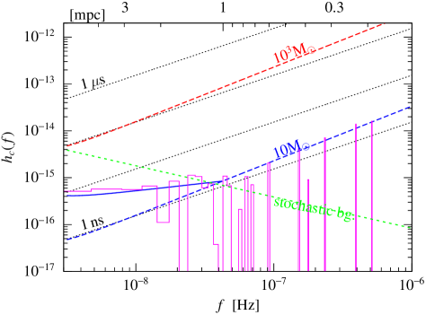
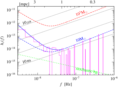
Figure 1 shows the orientation averaged characteristic GW amplitude for a 10 year observation, incorporating the additional near-field effects using Eqs. (24) and (27–30). The lower and top -axis shows the GW frequency and orbital radius for circular sources. The magenta curve displays the spectrum of timing residuals for a Monte Carlo realization of a population of 20,000 BHs within 1 pc with number density and random orientation with mass on circular orbits. The solid blue line shows the RMS foreground of a cusp of stellar mass BH averaged over different realizations. The spectrum separates into distinct spectral spikes at higher frequencies with RMS maxima shown by the dashed line. Figure 2 shows the GW amplitude of a realization of 1000 BHs with mass in 1 pc with a steeper number density profile . Despite of the smaller overall number of sources in the cluster, there are many more resolvable sources within 1 mpc in this case.
The net background level in Figures 1 and 2 is conservative, as the background is sensitive to the RMS mass of objects in the cluster, which may significantly exceed the mean. Furthermore, individual sources may generate up to larger timing residuals for certain orientations. Timing pulsars at a distance – from the Galactic Center with –s timing precision can be used to detect IMBHs of mass , if they exist within of SgrA∗. A population of stellar BHs within 2–5 mpc generates timing variations greater than 100 ns–10s for a pulsar within . However it will be much more difficult to individually resolve stellar BHs within to SgrA∗, which requires an extreme 1–20 ns timing precision.
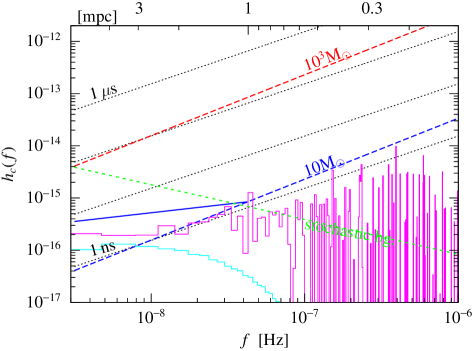
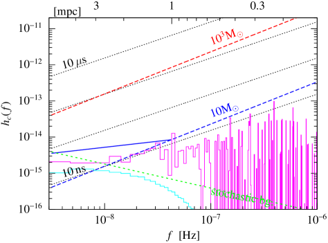
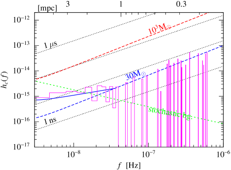
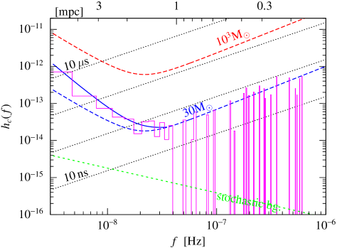
Figure 3 shows the characteristic GW spectra for a Monte Carlo realization of an eccentric population of BHs with an isotropic thermal eccentricity distribution. Magenta and cyan lines show the contribution of periodic and burst sources, respectively. The dashed lines show for individual circular sources, and the solid blue lines represent the RMS GW level for a population of circular sources for comparison. The net GW spectrum of burst sources is typically less than the level of periodic sources. The figure verifies the analytical calculations of Appendix A, the continuous low-frequency spectrum of periodic sources is indeed comparable to the circular level, modulo a weakly frequency dependent constant between . Note that for clarity, we are not including the gravitational near field effects here, which would dominate over the continuous low-frequency GW spectrum for as shown in Figure 1.
The transition to a spiky spectra happens at somewhat larger frequencies for eccentric sources (c.f. Figs. 1 and 3). Since individual sources generate GW spectra with many orbital upper harmonics, the net high frequency spectrum is more complicated than in the circular case. The orientation averaged spectral level for individual sources is typically less than per frequency bin, however, the total root-sum-squared signal of all upper harmonics of individual sources is much larger than the level of a single bin. In Appendix A we show that the SNR for detecting individual sources with a matched filter is comparable for eccentric and circular sources. In this sense, the dashed lines in Fig. 3, are representative of the total timing residual of individual sources as a function of pericenter frequency for arbitrary eccentricity. However, the full spectrum is rich in narrow features for eccentric sources and pericenter precession slowly modulates the amplitude of the timing residuals in individual pulsars. Both of these features could help to separate individual eccentric sources from the signal of other sources in GC.
6. Discussion
We have shown that pulsars within a few pc distance from the GC offer a unique probe to identify IMBHs and stellar BHs orbiting around SgrA∗. An IMBH, if present in the GC, sinks to orbital radii corresponding to the pulsar timing frequency bands. Depending on the binary orientation, orbital frequency, and pulsar distance, the GWs and gravitational near-field effects modulate the TOAs by a few ns to s for these sources with masses between and . Based on the GW spectral features, the signals of more than one IMBH (up to tens, if present) could be individually resolved and isolated from the fainter signal of stars and stellar mass objects and the cosmological GW background.
This observational probe is complimentary to EM measurements with different systematics. GWs are generated by all gravitating objects, including those that are black and undetectable in EM bands. GWs escape the galactic nucleus without any dissipation or dispersion. Closer to SgrA∗, sources generate stronger, higher frequency GWs, the number of observable cycles increases, and the number of objects per frequency bin decreases. Thus, unlike EM imaging techniques, the prospects for detecting and resolving individual objects through GW measurements improve closer in towards SgrA∗, even if the number density of objects increases inwards steeply. Furthermore, the gravitational effects are proportional to the RMS mass of objects, making the measurement more sensitive to individual higher mass objects in the distribution, even if the total mass of lighter objects is somewhat larger on comparable radius orbits.
Repeated pulsar timing observations over a few year baseline could reveal a detailed census of BHs in the inner mpc of the GC. We have shown that the GW foreground of stellar BHs rises above the cosmological background and separates into distinct peaks above nHz, corresponding to a GW period of less than 1 yr or orbital separations less than 1 mpc. Based on a simple estimate using circular orbits, we found that the total number of individually resolvable BHs is between 7–70, depending on the radial number density distribution exponent between and . These observations are therefore exponentially sensitive to , capable of testing the theory of strong mass segregation (Keshet et al., 2009).
Eccentricity complicates the spectral shape of resolvable sources by adding upper frequency harmonics. Although the timing residuals in individual frequency bins is suppressed by this effect relative to circular orbits, the total timing residual SNR with a matched filter is comparable for eccentric sources. At lower frequencies, a population of objects on eccentric orbits generates a stochastic GW foreground with a similar spectral shape and a comparable amplitude, as a circular population. Objects on larger-semimajor axis, eccentric orbits generate GW bursts during pericenter passage near SgrA∗. The stochastic GW burst signal is much less than the level of periodic sources.
This analysis hinges on the assumption that future surveys will discover pulsars near the GC that can be timed to the sufficient accuracy. Most of the observed S-stars within a few mpc and the young O/B stars in the GC will eventually turn into pulsars in a supernova explosion (Pfahl & Loeb, 2004). Based on the age and number of these stars, and assuming that we don’t live in a special time, one might expect more than pulsars in the GC. Some of these may become MSPs, and may be beamed towards us to be detectable with future SKA-type instruments (Cordes et al., 2004). They might be expected to segregate to the outskirts of the GC on a Gyr timescale as heavier objects sink inwards (Chanamé & Gould, 2002). Recently, Liu et al. (2012) examined the expected timing accuracy of pulsars in the GC accounting for radiometer noise, pulse phase jitter, and the interstellar scintillation of the ISM. They found that the timing accuracy of SKA is expected to be between – for regular pulsars. Our results indicate that the necessary accuracy to detect timing variations associated to individual BHs within 1 mpc requires much higher timing accuracy, which might be prohibitively difficult even with MSPs with a factor of 100–1000 better timing accuracy. However, the net variations caused by a population of these objects is detectable between 2–5 mpc at these accuracy levels. Remarkably, a – timing accuracy is sufficient to individually resolve or rule out the existence of IMBHs within 5 mpc from SgrA*.
As the GW spectrum is rich in strong spiky features at high frequencies, it may be possible to isolate GW induced timing residuals from other systematic effects. One such effect is if the pulsar itself is a part of a binary system. Fortunately, however, binaries with orbital periods of years, matching the GW foreground of the GC, are very soft, and are not long lived near the GC, they are easily disrupted by three-body encounters. Indeed, due to the high velocity dispersion in the GC, at , stellar mass binaries are soft for orbital frequencies , or orbital period day. The evaporation timescale on which a series of more distant encounters gradually increases the binary separation, is Myr, where is the Coulomb logarithm, and the ionization timescale to disrupt the binary by a close three body encounter is Myr (see § 7.5.7. in Binney & Tremaine 2008). Here we have expressed the binary semimajor axis with the orbital frequency, which is of order to match the GW signal. Thus, MSPs which form in short period binaries, like in typical LMXBs, and become wide, may be expected to typically become single in the GC. However, a few pulsar-BH binaries may form through three body exchange interactions and may be longer lived in the GC (Faucher-Giguère & Loeb, 2011). Ultimately, multiple pulsars would be necessary to rule out systematic effects.
GW observations with pulsar timing in the GC could be combined with other observable channels to map the GC. An IMBH orbiting around the SMBH would be observable with future millimeter VLBI imaging with EHT (Broderick et al., 2011). Conversely, if those observations reveal an IMBH, the inferred orbital parameters could help in identifying the GW counterpart with pulsar timing.
Appendix A Eccentric sources
Here we present the mathematical derivation of the GW foreground of eccentric sources in the GC. We start by reviewing the eccentric waveforms and GW spectra, then calculate the GW background of an eccentric population of periodic sources and burst sources, respectively, and finally discuss simple estimates of the signal-to-noise ratio of timing residuals for individual eccentric sources.
A.1. Waveform
An individual eccentric source with semimajor axis and eccentricity , generates a GW strain composed of discrete upper harmonics with frequency ,
| (A1) |
where
| (A2) |
where is the GW strain amplitude for circular orbits, and
| (A3) |
Here is the th Bessel function evaluated at (Peters & Mathews, 1963), and we have RMS averaged over the binary inclination. The Fourier transform of measured for some time is then
| (A4) |
Here is the Fourier transform of a window function of width and a unit integral. It approaches unity at and cuts off for . The spectral width of each GW harmonic is .
For circular sources, for and 0 otherwise. For eccentric sources, the dominant frequency harmonic is , the inverse pericenter passage timescale,
| (A5) |
where is the nearest integer larger than (O’Leary et al., 2009). The emitted GW spectrum is broadband with a maximum near , where and of the power is between and between , respectively. The harmonic weights in Eq. (A3) have a maximum near .
The definition of the inclination-averaged GW strain amplitude (A2) can be made more lucid by recalling the definition of the GW flux, , and verify if the total power output is consistent with Eq. (16) of Peters & Mathews (1963). Indeed,
| (A6) |
where we have used Kepler’s law , the definition of ,
| (A7) |
A.2. GW background of periodic sources
Let us estimate the net contribution of many sources to the GW background if observed for time . For a source with semimajor axis and eccentricity , the counts in each frequency bin are given by
| (A8) |
where is the GW frequency of the upper harmonic for a fixed semimajor axis. Conversely, the range of semimajor axis, , for which the harmonic contributes to the frequency bin between , is
| (A9) |
where .
Now let us assume a phase space distribution, in which the number of objects in the neighborhood of is . The number of sources that contribute to the harmonic is . The GW signal of all sources is then
| (A10) |
For periodic sources, is set by the condition that objects are observed for at least one orbit, , implying that . We shall consider the contribution of burst sources, on larger radius orbits observed for only a fraction of the orbit, separately below. Rearranging and using Eq. (A8), , and , gives
| (A11) |
Let us assume that . Then using and Eq. (A9), we find that the RHS is proportional to . Now let us express with using Eq. (A9),
| (A12) |
where
| (A13) |
Thus at , and increases monotonically, and asymptotes a constant for . One can show555To see this, consider an approximate sharply peaked signal around , for which , where if and 0 otherwise. that this constant is insensitive to the highest eccentricity sources if , which is expected to be satisfied. For and a thermal distribution of eccentricities , we get for . This together with Eq. (A12) shows that the net GW spectrum of a continuous population of eccentric sources is very similar to that of circular sources. However, the signal is much different for individually resolvable sources, as they are comprised of many upper harmonics
A.3. GW background of burst sources
GW bursts are generated by objects which make only one close approach near the SgrA* during the observation. These sources are on eccentric orbits with orbital time exceeding , but for which the pericenter timescale is less than and the orbital phase is such that pericenter passage occurs within the observation. The later condition means that only a fraction of all such sources will contribute in the observation time. For a fixed measurement frequency, , therefore , . Therefore and the fraction among these sources that contribute is .
Repeating the derivation for the net GW burst background over time , Eq. (A8–A10), we get
| (A14) |
where
| (A15) |
Note that resolving the burst source also requires that the sampling frequency and timescale between observations to satisfy and . This implies that has to hold. This requirement, however, is typically already satisfied for most sources if week, the number of sources on so eccentric orbits with such small , is close to zero. Comparing and , Eqs. (A13) and (A15), shows that the net GW signal of periodic sources exceeds the contribution of GW burst sources.
A.4. Signal to noise ratio
Here we present simple estimates on the scaling of the GW signal and timing SNR for eccentric sources using elementary functions. This is useful not only because the exact signal presented above is algebraically complicated, but also because the total SNR for individual sources is not represented well by in a single frequency bin, but it is sensitive to the coherent sum over many orbital harmonics.
Let us define an effective GW strain amplitude using that the GW power at pericenter passage, , is the average power times the fraction of time the source spends near pericenter passage, i.e. , given by Eq. (A5). Thus,
| (A16) |
This amounts to the root-sum-square of individual frequency harmonics in the spectrum for single sources, without averaging over the full orbit (c.f. Eq. (A6)). From this we get, that the effective strain at close passage is
| (A17) |
where and we have used . The pulsars are sensitive to the time integral of the strain (see § 4.2),
| (A18) |
The SNR is then where is the timing noise over time . Note that the RMS of the eccentricity dependent terms is 0.438 in Eq. (A18), if the eccentricity is drawn from a thermal distribution between (Binney & Tremaine, 2008). The SNR of the timing residual is not very sensitive to the semimajor axis, or the maximum eccentricity in the cluster. For fixed , eccentric sources contribute to the net timing residuals at a similar level as circular sources.
Eq. (A18) is only applicable for periodic sources, i.e. if . For a single GW burst source with ,
| (A19) |
provided that the orbital phase coincides with pericenter passage during the observation. This shows that for burst sources with fixed pericenter distance, the total timing residual is weakly dependent on eccentricity, for fixed pericenter distance. The number of sources is constant as a function of for fixed , but the fraction of sources that are near pericenter passage at any given instant decreases quickly for smaller proportional to . Therefore the net contribution of burst sources scales as
| (A20) |
The spectral density within a frequency bin follows from implying that . The average timing spectral density of burst sources decreases quickly toward higher frequencies.
References
- Alexander & Hopman (2009) Alexander, T., & Hopman, C. 2009, ApJ, 697, 1861
- Alvi (2000) Alvi, K. 2000, Phys. Rev. D, 61, 124013
- Bahcall & Wolf (1976) Bahcall, J. N., & Wolf, R. A. 1976, ApJ, 209, 214
- Bates et al. (2011) Bates, S. D., et al. 2011, MNRAS, 411, 1575
- Baumgardt et al. (2006) Baumgardt, H., Gualandris, A., & Portegies Zwart, S. 2006, MNRAS, 372, 174
- Binney & Tremaine (2008) Binney, J., & Tremaine, S. 2008, Galactic Dynamics: Second Edition (Princeton University Press)
- Blanchet et al. (1998) Blanchet, L., Faye, G., & Ponsot, B. 1998, Phys. Rev. D, 58, 124002
- Blandford et al. (1987) Blandford, R. D., Romani, R. W., & Applegate, J. H. 1987, MNRAS, 225, 51P
- Broderick et al. (2011) Broderick, A. E., Loeb, A., & Reid, M. J. 2011, ApJ, 735, 57
- Chanamé & Gould (2002) Chanamé, J., & Gould, A. 2002, ApJ, 571, 320
- Cordes (2007) Cordes, J. 2007, Pulsar searches and timing with the SKA, http://www.skatelescope.org/
- Cordes et al. (2004) Cordes, J. M., Kramer, M., Lazio, T. J. W., Stappers, B. W., Backer, D. C., & Johnston, S. 2004, New A Rev., 48, 1413
- Cornish (2009) Cornish, N. J. 2009, Phys. Rev. D, 80, 087101
- Davis et al. (2011) Davis, S. W., Narayan, R., Zhu, Y., Barret, D., Farrell, S. A., Godet, O., Servillat, M., & Webb, N. A. 2011, ApJ, 734, 111
- de Paolis et al. (1996) de Paolis, F., Gurzadyan, V. G., & Ingrosso, G. 1996, A&A, 315, 396
- Deneva et al. (2009) Deneva, J. S., Cordes, J. M., & Lazio, T. J. W. 2009, ApJ, 702, L177
- Detweiler (1979) Detweiler, S. 1979, ApJ, 234, 1100
- Faucher-Giguère & Loeb (2011) Faucher-Giguère, C.-A., & Loeb, A. 2011, MNRAS, 911
- Finn (2009) Finn, L. S. 2009, Phys. Rev. D, 79, 022002
- Freitag et al. (2006a) Freitag, M., Amaro-Seoane, P., & Kalogera, V. 2006a, ApJ, 649, 91
- Freitag et al. (2006b) Freitag, M., Gürkan, M. A., & Rasio, F. A. 2006b, MNRAS, 368, 141
- Fritz et al. (2010) Fritz, T. K., et al. 2010, ApJ, 721, 395
- Fujii et al. (2009) Fujii, M., Iwasawa, M., Funato, Y., & Makino, J. 2009, ApJ, 695, 1421
- Genzel et al. (2010) Genzel, R., Eisenhauer, F., & Gillessen, S. 2010, Reviews of Modern Physics, 82, 3121
- Gillessen et al. (2009) Gillessen, S., Eisenhauer, F., Trippe, S., Alexander, T., Genzel, R., Martins, F., & Ott, T. 2009, ApJ, 692, 1075
- Gualandris et al. (2010) Gualandris, A., Gillessen, S., & Merritt, D. 2010, MNRAS, 409, 1146
- Gualandris & Merritt (2009) Gualandris, A., & Merritt, D. 2009, ApJ, 705, 361
- Gualandris & Merritt (2012) —. 2012, ApJ, 744, 74
- Gualandris et al. (2005) Gualandris, A., Portegies Zwart, S., & Sipior, M. S. 2005, MNRAS, 363, 223
- Hansen & Milosavljević (2003) Hansen, B. M. S., & Milosavljević, M. 2003, ApJ, 593, L77
- Hobbs et al. (2010) Hobbs, G., et al. 2010, Classical and Quantum Gravity, 27, 084013
- Iwasawa et al. (2011) Iwasawa, M., An, S., Matsubayashi, T., Funato, Y., & Makino, J. 2011, ApJ, 731, L9
- Jaffe & Backer (2003) Jaffe, A. H., & Backer, D. C. 2003, ApJ, 583, 616
- Jenet et al. (2009) Jenet, F., et al. 2009, arXiv:0909.1058
- Jenet et al. (2005) Jenet, F. A., Creighton, T., & Lommen, A. 2005, ApJ, 627, L125
- Jenet et al. (2004) Jenet, F. A., Lommen, A., Larson, S. L., & Wen, L. 2004, ApJ, 606, 799
- Johnson-McDaniel et al. (2009) Johnson-McDaniel, N. K., Yunes, N., Tichy, W., & Owen, B. J. 2009, Phys. Rev. D, 80, 124039
- Johnston et al. (2006) Johnston, S., Kramer, M., Lorimer, D. R., Lyne, A. G., McLaughlin, M., Klein, B., & Manchester, R. N. 2006, MNRAS, 373, L6
- Keith et al. (2011) Keith, M. J., Johnston, S., Levin, L., & Bailes, M. 2011, MNRAS, 948
- Keshet et al. (2009) Keshet, U., Hopman, C., & Alexander, T. 2009, ApJ, 698, L64
- Khan et al. (2011) Khan, F. M., Just, A., & Merritt, D. 2011, ApJ, 732, 89
- Kocsis & Levin (2011) Kocsis, B., & Levin, J. 2011, arXiv:1109.4170
- Kocsis & Sesana (2011) Kocsis, B., & Sesana, A. 2011, MNRAS, 411, 1467
- Königsdörffer & Gopakumar (2006) Königsdörffer, C., & Gopakumar, A. 2006, Phys. Rev. D, 73, 124012
- Kramer et al. (1998) Kramer, M., Xilouris, K. M., Lorimer, D. R., Doroshenko, O., Jessner, A., Wielebinski, R., Wolszczan, A., & Camilo, F. 1998, ApJ, 501, 270
- Lazio & Cordes (1998) Lazio, T. J. W., & Cordes, J. M. 1998, ApJ, 505, 715
- Liu et al. (2012) Liu, K., Wex, N., Kramer, M., Cordes, J. M., & Lazio, T. J. W. 2012, ApJ, 747, 1
- Lommen & Backer (2001) Lommen, A. N., & Backer, D. C. 2001, ApJ, 562, 297
- Macquart et al. (2010) Macquart, J.-P., Kanekar, N., Frail, D. A., & Ransom, S. M. 2010, ApJ, 715, 939
- Madau & Rees (2001) Madau, P., & Rees, M. J. 2001, ApJ, 551, L27
- Maillard et al. (2004) Maillard, J. P., Paumard, T., Stolovy, S. R., & Rigaut, F. 2004, A&A, 423, 155
- Matsubayashi et al. (2007) Matsubayashi, T., Makino, J., & Ebisuzaki, T. 2007, ApJ, 656, 879
- Merritt et al. (2009) Merritt, D., Gualandris, A., & Mikkola, S. 2009, ApJ, 693, L35
- Miller & Colbert (2004) Miller, M. C., & Colbert, E. J. M. 2004, International Journal of Modern Physics D, 13, 1
- Miralda-Escudé & Gould (2000) Miralda-Escudé, J., & Gould, A. 2000, ApJ, 545, 847
- Morris (1993) Morris, M. 1993, ApJ, 408, 496
- O’Leary et al. (2009) O’Leary, R. M., Kocsis, B., & Loeb, A. 2009, MNRAS, 395, 2127
- O’Leary et al. (2006) O’Leary, R. M., Rasio, F. A., Fregeau, J. M., Ivanova, N., & O’Shaughnessy, R. 2006, ApJ, 637, 937
- Peters (1964) Peters, P. C. 1964, Physical Review, 136, 1224
- Peters & Mathews (1963) Peters, P. C., & Mathews, J. 1963, Physical Review, 131, 435
- Pfahl & Loeb (2004) Pfahl, E., & Loeb, A. 2004, ApJ, 615, 253
- Phinney (2001) Phinney, E. S. 2001, ArXiv eprints, astro-ph/0108028
- Portegies Zwart et al. (2006) Portegies Zwart, S. F., Baumgardt, H., McMillan, S. L. W., Makino, J., Hut, P., & Ebisuzaki, T. 2006, ApJ, 641, 319
- Portegies Zwart & McMillan (2002) Portegies Zwart, S. F., & McMillan, S. L. W. 2002, ApJ, 576, 899
- Preto et al. (2011) Preto, M., Berentzen, I., Berczik, P., & Spurzem, R. 2011, ApJ, 732, L26
- Rajagopal & Romani (1995) Rajagopal, M., & Romani, R. W. 1995, ApJ, 446, 543
- Ray & Kluzniak (1994) Ray, A., & Kluzniak, W. 1994, in IAU Symposium, Vol. 165, GA XXII, VT.145, ed. H. van Woerden
- Reid & Brunthaler (2004) Reid, M. J., & Brunthaler, A. 2004, ApJ, 616, 872
- Sesana (2010) Sesana, A. 2010, ApJ, 719, 851
- Sesana et al. (2004) Sesana, A., Haardt, F., Madau, P., & Volonteri, M. 2004, ApJ, 611, 623
- Sesana et al. (2008) Sesana, A., Vecchio, A., & Colacino, C. N. 2008, MNRAS, 390, 192
- Sesana et al. (2009) Sesana, A., Vecchio, A., & Volonteri, M. 2009, MNRAS, 394, 2255
- Smits et al. (2009) Smits, R., Kramer, M., Stappers, B., Lorimer, D. R., Cordes, J., & Faulkner, A. 2009, A&A, 493, 1161
- Smits et al. (2011) Smits, R., Tingay, S. J., Wex, N., Kramer, M., & Stappers, B. 2011, A&A, 528, A108+
- van Haasteren et al. (2011) van Haasteren, R., et al. 2011, MNRAS, 414, 3117
- Wex et al. (1996) Wex, N., Gil, J., & Sendyk, M. 1996, A&A, 311, 746
- Wyithe & Loeb (2003) Wyithe, J. S. B., & Loeb, A. 2003, ApJ, 590, 691
- Yu & Tremaine (2003) Yu, Q., & Tremaine, S. 2003, ApJ, 599, 1129