Abstract

We study the top pair production cross section at the LHC in the context of Randall-Sundrum model including the Kaluza-Klein (KK) excited gravitons. It is shown that the recent measurement of the cross section of this process at the LHC restricts the parameter space in Randall-Sundrum (RS) model considerably. We show that the coupling parameter ($\frac{k}{\overline{M}_{pl}}$) is excluded by this measurement from $0.03$ to $0.22$ depending on the mass of first KK excited graviton ($m_{1}$). We also study the effect of KK excitations on the spin correlation of the top pairs. It is shown that the spin asymmetry in $t\bar{t}$ events is sensitive to the RS model parameters with a reasonable choice of model parameters.

1 Introduction

One of the primary mysteries of high energy physics is the large difference between scale of the electroweak and fundamental scale of gravity which is known as the hierarchy problem. One way to solve the hierarchy problem was proposed by Randall and Sundrum (RS) in 1999 [1]. In this model, gravity can propagate in 5-dimensional non-factorizable geometry and therefore it generates the 4-dimensional weak Planck scale hierarchy by an exponential function of the compactification radius which is called warped factor. In this scenario, an infinite tower of the KK excited particles appears which their effective couplings with other particles are characterized by an exponential warped factor. While in the Arkani-Hamed, Dimopoulos and Dvali (ADD) model for extra dimension [2], the mass difference of each KK excited particle is inversely proportional to the radius of the extra dimensions and it is more difficult to detect and identify the KK excited particles at the LHC. As a consequence, the RS model is more motivated than the ADD model [2].

The top quark is the heaviest fundamental particle which have been discovered to date and might be the first place in which the new physics effects could appear. The LHC allows us to investigate the properties of the top quark in details. Very large numbers of top quarks are produced at the LHC eventually more than $10^{7}$ $t\overline{t}$ pairs per year [3]. This will make feasible the precise investigations of the top interactions. At the LHC, top quarks are dominantly produced in $t\overline{t}$ pairs via the processes $q\overline{q}\rightarrow t\overline{t}$ and $gg\rightarrow t\overline{t}$. An intriguing speciality of the top quark is its extremely short lifetime which is due to its heaviness. This feature causes that it decays before it can form any hadronic bound state. As a result, the top quark spin will be transferred to its decay products.

The cross section value for top pair production have been measured by CMS experiment recently [4]:

$$\sigma(pp\rightarrow t{\overline{t}}) =165.8\pm 13.3~{}[pb]~{}(\rm stat\oplus sys).$$ (1)

In this paper, we study the effects of RS model on the $t\overline{t}$ production at the LHC and compare our numerical results with the experimental measurement. To study the effects of RS model, we consider three quantities which are particularly useful for comparing theory with experimental results. These quantities are the total cross section of top pair production, the differential cross section as a function of invariant mass of $t\bar{t}$, and the spin asymmetry in top-antitop production.

The rest of this paper is organized as follows: In the next section, we summarize the effects of RS model on the cross section production of top-antitop and spin asymmetry. In section 3 we compare the effects of the RS model with the LHC measurements and present our numerical results. In section 3, we also discuss the constraints on the parameters space of RS model using the future measurements of spin asymmetry. The conclusions are given in section 4.

2 The effects of RS model on $t\bar{t}$ production

In this section, we briefly describe the model and study the effects of KK excited gravitons on top-antitop production at the LHC. The set up of RS model consists of two D3-branes which embedded in a five dimensional bulk spacetime [1]. This theory has been considered a 5-dimensional non-factorizable metric [1]:

$$ds^{2}=e^{-2kr_{c}\pi}\eta_{\mu\nu}dx^{\mu}dx^{\nu}-r_{c}^{2}d\phi^{2},$$ (2)

where $x_{\mu}$ are the coordinates for the familiar four dimensions, $\phi$ ($0\leq\phi\leq\pi$) is the coordinate for an extra dimension and $r_{c}$ is a compactification radius. Two branes are localized at $\phi=0$ and $\pi$ which are called hidden and visible branes, respectively. Here $k$ is the $\rm AdS$ curvature scale which is of order the Planck scale.

Effective Lagrangian in 4-dimensional effective theory is given by [5]:

$${\cal{L}}_{int} = -\frac{1}{M^{3/2}}T^{\alpha\beta}(x)h_{\alpha\beta}(x,\phi=\pi),$$ (3)

where $M$ is the known Planck scale, $T_{\alpha\beta}$ is the symmetric energy-momentum tensor of the SM fields on the visible brane and $h_{\alpha\beta}$ are graviton fields. After expanding the graviton field into the KK states, Lagrangian is found as:

$${\cal{L}}_{int} = -\frac{1}{\overline{M}_{pl}}T^{\alpha\beta}(x)h^{(0)}_{\alpha\beta}-\frac{1}{\Lambda{{}_{\pi}}}T^{\alpha\beta}(x)\sum_{n=1}^{\infty}h^{(n)}_{\alpha\beta}(x),$$ (4)

where $\overline{M}_{pl}$ is the reduced Planck mass. Examining of the RS action in the 4-D effective theory yields the relation:

$$\overline{M}^{2}_{Pl}=\frac{{M}^{3}}{k}(1-e^{-2kr_{c}\pi}).$$ (5)

To solve the hierarchy problem, it is assumed that gravity is localized on the brane at $\phi=0$ and $kr_{c}\simeq 11-12$ [5]. In this situation, $\rm TeV$ scale theory can naturally be attained on the 3-brane at $\phi=\pi$. The scale of physical processes on this $\rm TeV$-brane is then $\Lambda_{\pi}\equiv\overline{M}_{pl}e^{-kr_{c}\pi}$. According to Eq. 4, the graviton zero-mode couples to the SM fields with usual strength while the KK modes strongly couples to the SM fields with the suppression factor of $1/\Lambda_{\pi}$.

The masses of the KK excitations of graviton are given by:

$$m_{n} =x_{n}ke^{-kr_{c}\pi},\$$ (6)

where $x_{n}$ is a root of the Bessel function of the first order. In this paper, we study the effect of exchanged KK excited gravitons on the $t\bar{t}$ production cross section. The leading order (LO) processes for the production of top pair at the LHC include these two processes $q\overline{q}\rightarrow t\overline{t}$ and $gg\rightarrow t\overline{t}$. The corresponding invariant matrix elements for these processes including the KK graviton modes effects have been calculated in [7, 8, 9]. When $q\overline{q}$ is the initial state, the amplitude for the same spin direction of top-antitop and opposite spin direction are given by:

$$|{\cal{M}}(q\overline{q}\rightarrow t_{\uparrow}\overline{t}_{\uparrow})|^{2} = |{\cal{M}}(q\overline{q}\rightarrow t_{\downarrow}\overline{t}_{\downarrow})|^{2}$$ (7)

$$= \frac{g^{4}}{9}(1-\beta^{2})\sin^{2}\theta+\frac{|A(s)|^{2}s^{4}\beta^{2}}{128}(1-\beta^{2})\sin 2\theta,$$

$$|{\cal{M}}(q\overline{q}\rightarrow t_{\uparrow}\overline{t}_{\downarrow})|^{2} = |{\cal{M}}(q\overline{q}\rightarrow t_{\downarrow}\overline{t}_{\uparrow})|^{2}$$ (8)

$$= \frac{g^{4}}{9}(1+\cos^{2}\theta)+\frac{|A(s)|^{2}s^{4}\beta^{2}}{128}(\cos^{2}2\theta+\cos^{2}\theta),$$

where $\beta=\sqrt{1-4m_{t}^{2}/s}$ and $m_{t}$ is the top quark mass. Here $A(s)$ is defined by

$$A(s)=-\frac{1}{\Lambda^{2}_{\pi}}\sum_{n=1}^{\infty}\frac{1}{s^{2}-m^{2}_{n}+im_{n}\Gamma_{n}},$$ (9)

where $s$ is partonic centre-of-mass energy and $\Gamma_{n}$ is the total decay width of the $n$-th KK graviton excitation [7]. In this paper, we take to account the effects of KK excited gravitons up to $n=5$. For larger values of $m_{n}$, the effects of KK excitations on observables are negligible. In Eq. 7, $\theta$ is the angle between the incoming and outgoing top quark, $g$ is the strong coupling constant. For the situation with gluon-gluon in the initial states, the amplitude is given by:

$$|{\cal{M}}(gg\rightarrow t_{\uparrow}\overline{t}_{\uparrow})|^{2} = |{\cal{M}}(gg\rightarrow t_{\downarrow}\overline{t}_{\downarrow})|^{2}$$ (10)

$$= \frac{g^{4}\beta^{2}}{96}{\cal{D}}(\beta,\cos\theta)(1-\beta^{2})(1+\beta^{2}+\beta^{2}\sin^{4}\theta)$$

$$+ {\cal{Z}}(\beta,\theta,s)s^{2}\beta^{2}(1-\beta^{2})\sin^{4}\theta,$$

$$|{\cal{M}}(gg\rightarrow t_{\uparrow}\overline{t}_{\downarrow})|^{2} = |{\cal{M}}(gg\rightarrow t_{\downarrow}\overline{t}_{\uparrow})|^{2}$$ (11)

$$= \frac{g^{4}\beta^{2}}{96}{\cal{D}}(\beta,\cos\theta)\sin^{2}\theta(1+\cos^{2}\theta)$$

$$+ {\cal{Z}}(\beta,\theta,s)s^{2}\beta^{2}\sin^{2}\theta(1+\cos^{2}\theta).$$

In the above Equations, ${\cal{D}}(\beta,\cos\theta)$ and ${\cal{Z}}(\beta,\theta,s)$ are defined by:

$${\cal{D}}(\beta,\cos\theta)=\frac{7+9\beta^{2}\cos^{2}\theta}{(1-\beta^{2}\cos^{2}\theta)^{2}},$$ (12)

$${\cal{Z}}(\beta,\theta,s)=\frac{1}{32}(-\frac{g^{2}}{1-\beta^{2}\cos^{2}\theta}\rm Re(A(s))+\frac{3}{8}|A(s)|^{2}s^{2}).$$ (13)

The total cross section for production of $t\bar{t}$ with spin indices $\alpha$ and $\beta$ has the following form:

$$\sigma(pp\rightarrow t_{\alpha}{\overline{t}}_{\beta}) = \sum_{ab}\int dx_{1}dx_{2}f_{a}(x_{1},Q^{2})f_{b}(x_{2},Q^{2})\widehat{\sigma}(ab\rightarrow t_{\alpha}{\overline{t}}_{\beta}),\$$ (14)

where $f_{a,b}(x_{i},Q^{2})$ are the parton structure functions of proton. $x_{1}$ and $x_{2}$ are the parton momentum fractions and $Q$ is the factorization scale.

3 Numerical results

In the previous section, we introduced the total cross section of top pair production at the LHC. In this section, we calculate the differential cross section and spin asymmetry and compare them with the ongoing measurement at the LHC.

We are also interested in the differential cross section as a function of invariant mass $M_{t\overline{t}}=\sqrt{(p_{t}+p_{\overline{t}})^{2}}$, where $p_{t}$ and $p_{\overline{t}}$ are the four-momenta of top and anti-top, respectively. This quantity is defined by

$$\frac{d\sigma(pp\rightarrow t_{\alpha}\overline{t}_{\beta})}{dM_{t\overline{t}}}=\sum_{ab}\int_{\frac{M^{2}_{t\overline{t}}}{E^{2}_{CMS}}}^{1}dx_{1}\frac{2M^{2}_{t\overline{t}}}{x_{1}E^{2}_{CMS}}f_{a}(x_{1},Q^{2})f_{b}(\frac{M^{2}_{t\overline{t}}}{x_{1}E^{2}_{CMS}},Q^{2})\widehat{\sigma}(ab\rightarrow t_{\alpha}{\overline{t}}_{\beta}).$$ (15)

The best way to study the top pair spin correlation is to analyze the angular correlations of two charged leptons originating from the full leptonic top-antitop decay. Spin asymmetry between the top-antitop pair is defined as [10]:

$$A=\frac{\sigma_{\uparrow\uparrow}+\sigma_{\downarrow\downarrow}-\sigma_{\uparrow\downarrow}-\sigma_{\downarrow\uparrow}}{\sigma_{\uparrow\uparrow}+\sigma_{\downarrow\downarrow}+\sigma_{\uparrow\downarrow}+\sigma_{\downarrow\uparrow}}$$ (16)

where $\sigma_{\uparrow/\downarrow\uparrow/\downarrow}$ are the production cross section for top pair with characterized spin indices. In the context of SM, spin asymmetry has been calculated at $7~{}\rm TeV$ center-of-mass energy to be $0.16$ for the LHC while it is $0.32$ for $14~{}\rm TeV$. The CMS collaboration hopes to measure spin asymmetry of this process by several percent [11].

In the rest of this section, we study the effects of KK excitation of gravitons on the production cross section of $pp\rightarrow t\overline{t}$ at the LHC. We first discuss the bounds on parameters space of the RS model then we present our results and discuss the possibility of restricting the RS model parameters at the LHC via top pair production observables.

In the RS model, there are two main parameters which are the first excitation graviton mass ($m_{1}$) and the coupling parameter ($\frac{k}{\overline{M}_{pl}}$). There are two kinds of experimental constraints on the parameters of RS model. First kind of constraints arises from indirect searches for the large extra dimensions. Model dependent limits can be placed on the masses of KK excitation fields from the precision electroweak tests [12], cosmology ($e.g$., expansion rate of the universe) [14], black hole production at colliders [15], flavor observables and Higgs related collider searches [13], and low energy experiments ($e.g.$, CP violation and FCNC processes) [16]. Another kind of constraints comes from the direct searches for KK gravitons at Tevatron [17] and LHC [18, 19]. In [18], RS gravitons decaying to pairs of photons have been studied and shown that for values of the coupling parameter ($\frac{k}{\overline{M}_{pl}}$) ranging from 0.01 to 0.1, at $95\%$ confidence level, the lower bounds on excited graviton masses vary from than 371 to $945~{}\rm GeV$. Paper [19] describes a search for high mass resonance decaying to electron pairs. It is shown that the corresponding limits on RS graviton production for coupling of $0.1$ and $0.05$ are 930 and $730~{}\rm GeV$, respectively.

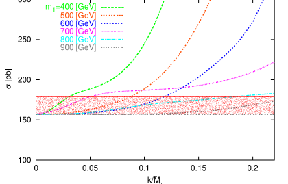
Figure 1: The total cross section of $t\bar{t}$ production at the LHC as a function of $\frac{k}{\overline{M}_{pl}}$. The horizontal dotted black line at 157 $~{}\rm pb$ depicts the theoretical SM value and dotted red line at $179.1~{}\rm pb$ depicts the present upper experimental limit on the cross section.

In this paper, to calculate $\sigma(pp\rightarrow t\overline{t})$, we have used the MSTW parton structure functions [20] and set the center-of-mass energy to $7~{}\rm TeV$. To study the effects of KK excited gravitons on top-antitop production, we display the cross section of $pp\rightarrow t\overline{t}$ versus $\frac{k}{\overline{M}_{pl}}$ in Figure-1. In Fig. 1, we have considered different values for $m_{1}$. The horizontal dotted black line at $157$ $\rm pb$ depicts the theoretical SM prediction and the dotted red line at $179.1$ $\rm pb$ depicts the present upper experimental limit on the cross section. Obviously, all curves asymptotically tend to the SM prediction when $\frac{k}{\overline{M}_{pl}}\rightarrow 0$. Fig. 1 shows that for the region of $\sigma(pp\rightarrow t\overline{t})$ above the present experimental bound, coupling parameter ($\frac{k}{\overline{M}_{pl}}$) is excluded. Hatched area shows values for $\frac{k}{\overline{M}_{pl}}$ which have not been excluded by the present upper experimental limit. Notice that for various values of $m_{1}$, bounds on $\frac{k}{\overline{M}_{pl}}$ are different but this dependence is not linear. As it can be seen in Fig.1, for excited graviton masses of $m_{1}=$ 400, 500, 600, 700, 800 and $900~{}\rm GeV$, the values of the coupling parameter ($\frac{k}{\overline{M}_{pl}}$) must be smaller than 0.02, 0.06, 0.1, 0.035, 0.11 and 0.2, respectively. The limits are stronger than some of the bounds coming from other approaches [18, 19].

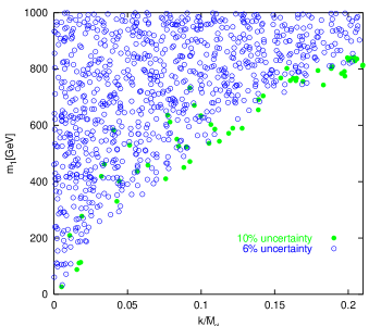
Figure 2: Scatter plot of $m_{1}$ versus $\frac{k}{\overline{M}_{pl}}$. Plot is showing the points (filled and empty) for which the total cross section of top-antitop production are in the range of experimental uncertainty as mentioned in relation (1). The points depicted by filled circle (green) are the region where the total cross section of top-antitop production are in the range of the present precision experimental limit with $10\%$ uncertainty. The points depicted by empty circle (blue) show the points at which the total cross section of top-antitop production is in the range that can be probed in near future with $6\%$ uncertainty.

To illustrate this observation, we have shown a scatter plot in Fig.2. This diagram depicts scatter plot of $m_{1}$ versus $\frac{k}{\overline{M}_{pl}}$. Fig.2 is showing the points (filled and empty) for which the total cross section of top-antitop production are in the range of experimental uncertainty as mentioned in relation (1). For drawing this plot, we have selected various random values for $m_{1}$ and $\frac{k}{\overline{M}_{pl}}$. At points marked by filled circle (green), the total cross section of top-antitop production corresponds to the present precision of the experimental measurement in relation (1). The scatter points depicted by empty circles (blue) are the points that the total cross section of top-antitop production correspond to the range that can be probed in near future with $6\%$ uncertainty. If we assume to measure the top pair cross section with $6\%$ uncertainty, the filled circle will be excluded. The future experimental uncertainty of the LHC on the cross section measurement of top-antitop provides slightly better constraints on the value of on the value of $\frac{k}{\overline{M}_{pl}}$, as shown in also shows that by increasing value of the $m_{1}$, constraints on value of the $m_{1}$, constraints on $\frac{k}{\overline{M}_{pl}}$ will

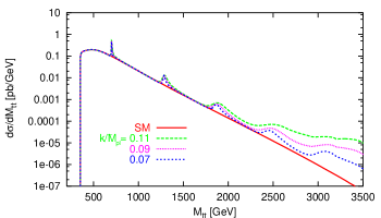
Figure 3: Differential cross section of top-antitop production at the LHC as a function of invariant mass $M_{t\overline{t}}$. We have set $m_{1}=700$ GeV and considered different values for $\frac{k}{\overline{M}_{pl}}$. The red curve, dashed (green) curve, small dotted (pink) curve and large dotted (blue) curve respectively correspond to SM, and RS model with $\frac{k}{\overline{M}_{pl}}=$ 0.11, 0.09 and 0.07.

In Fig. 3, we have displayed the differential cross section of top-antitop production at LHC as a function of invariant mass of top pair $M_{t\bar{t}}$. In this figure, $m_{1}=700$ GeV and considered different values for $\frac{k}{\overline{M}_{pl}}$. The red curve, dashed (green) curve, small dotted (pink) curve and large dotted (blue) curve correspond to the SM prediction, and the RS model with $\frac{k}{\overline{M}_{pl}}=$ 0.11, 0.09 and 0.07, respectively. As it is shown, there are large deviations around the masses of KK excited garvitons in the RS model from the SM prediction. So far, $t\overline{t}$ invariant mass distribution has not been analyzed to search for RS model. Similar analysis for SM-like $Z^{\prime}$ has been performed at the LHC [21] but with dielectron final state. In [21], no significant deviation from the SM expectation has been observed.

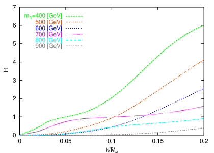
Figure 4: Relative change in spin asymmetry of top-antitop production at the LHC as a function of $\frac{k}{\overline{M}_{pl}}$. We have considered different values of $m_{1}$.

The top quark spin asymmetry in dilepton channel at the LHC is predicted with a small uncertainty in the SM [11]. For this reason, the spin correlation in $t\bar{t}$ production at the LHC is a good way to search for beyond SM. For a better study of RS model, we consider the relative change in spin asymmetry which is defind as:

$$R=\frac{A-A_{SM}}{A_{SM}},\$$ (17)

where $A$ is spin asymmetry in the presence of KK excited gravitons and $A_{SM}$ is the SM prediction for spin asymmetry. The relative change in spin asymmetry of the top-antitop production at the LHC as a function of $\frac{k}{\overline{M}_{pl}}$ is shown in Fig. 4. In this figure, we have considered different values of $m_{1}$.

In [22], it has been shown that a $4\%$ precision on spin asymmetry measurement of $t\overline{t}$ production at the LHC is possible with $10~{}\rm fb^{-1}$ . As it can be seen in Fig. 4, deviations from SM prediction in RS model can be large depending on the model parameters. Therefore, measurement of spin asymmetry in $t\overline{t}$ pair production can help us probe new physics effects.

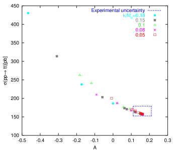
Figure 5: Scatter plot of the total cross section of $t\overline{t}$ pair production at the LHC versus spin asymmetry.

Fig. 5 is the scatter plot of $t\bar{t}$ production cross section at the LHC versus the spin asymmetry. This plot is showing different values for the total cross section of top-antitop and spin asymmetry in situation that various inputs have been selected for $m_{1}$ and $\frac{k}{\overline{M}_{pl}}$. The rectangle shows the present experimental uncertainty for the total cross section (relation 1) and the possible precision of the spin asymmetry measurement with the SM predictions in center [11]. As it can be seen in Fig. 5, there are several points which their total cross sections and spin asymmetry do not violate experimental bounds and therefore there is a hope to observe RS effects at the LHC.

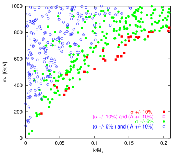
Figure 6: Scatter plot of $m_{1}$ versus $\frac{k}{\overline{M}_{pl}}$. Scatter plot is showing the points (filled and empty) for which the total cross section of top pair production correspond to the present and future experimental uncertainties without and with including possible spin asymmetry measurement around the SM prediction.

In order to obtain stronger bounds on $m_{1}$ and $\frac{k}{\overline{M}_{pl}}$, we have simultaneously considered cross section and spin asymmetry in $t\overline{t}$ pair production in Fig. 6. In Fig. 6, we have drawn a scatter plot of $m_{1}$ versus $\frac{k}{\overline{M}_{pl}}$. The scatter plot is showing points (filled and empty) for which the total cross section of top pair production correspond to the experimental uncertainty measurement as it is mentioned in relation 1 and spin asymmetry is within the future uncertainty of $10\%$. Notice that $m_{1}$ and $\frac{k}{\overline{M}_{pl}}$ have been generated randomly. The empty squares (pink) in Fig. 6 are the points at which the total cross section of top-antitop production corresponds to the experimental uncertainty as mentioned in relation (1), and the spin asymmetry is in the range of SM and the spin asymmetry is in the range of SM prediction with point which can satisfy these conditions. This means that by measuring spin asymmetry with $10\%$ uncertainty, we can derive new bounds on RS parameters. The filled squares (red) show similar situation except that we relax any constraints coming from spin asymmetry. The points depicted by empty circles (blue) are the points at which the total cross section of top-antitop production is in the range which can be probed in near future with $6\%$ uncertainty and the spin asymmetry is in the range of SM prediction with $10\%$ uncertainty. If we assume to measure the cross section of $t\overline{t}$ with $6\%$ uncertainty, the filled squares will be excluded. The filled circles (green) are similar to blue circles except that we relax any constraints coming from spin asymmetry. This figure shows, with simultaneous measurement of the total cross section and spin asymmetry of top-antitop production at the LHC, we can derive stronger bounds on $\frac{k}{\overline{M}_{pl}}$ in comparison with using single measurement of total cross section. It also can be seen that for large values of $m_{1}$, limits are weaker.

4 Concluding remarks

In this paper, we have studied the effects of KK excited gravitons on $t\bar{t}$ production cross section at the LHC with the center-of-mass energy of $\sqrt{s}=7~{}\rm TeV$. We have shown that the contribution of this model to the cross section production of $t\overline{t}$ can exceed the present experimental measurement. From this observation the parameter space of RS model is restricted. We have shown that for the excited graviton masses $m_{1}=$ 400, 500, 600, 700, 800 and $900~{}\rm GeV$, the values of the coupling parameter ($\frac{k}{\overline{M}_{pl}}$) must be smaller than 0.02, 0.06, 0.1, 0.035, 0.11 and 0.2, respectively. Also we showed that for various values of $m_{1}$, restriction on restriction on $\frac{k}{\overline{M}_{pl}}$ can be different but this completely linear and with the growth of $m_{1}$, it does not decrease in all regions. The limits on RS parameters which arise from studying of production cross section of top-antitop can be stronger than the ones obtained from other approaches.

Assuming a relative uncertainty of $6\%$ on the measurement of cross section of top-antitop in near future measurement at LHC, We have shown $\frac{k}{\overline{M}_{pl}}$ can slightly be constrained. We discussed that using the spin asymmetry $A$, one can derive stronger bound on coupling parameter ($\frac{k}{\overline{M}_{pl}}$).

References

- [1] L. Randall and R. Sundrum, Phys. Rev. Lett. 83 (1999) 3370 [arXiv:hep-ph/9905221]; L. Randall and R. Sundrum, Phys. Rev. Lett. 83 (1999) 4690 [arXiv:hep-th/9906064].
- [2] N. Arkani-Hamed, S. Dimopoulos and G. R. Dvali, Phys. Lett. B 429 (1998) 263 [arXiv:hep-ph/9803315].
- [3] E. Halkiadakis, arXiv:1004.5564 [hep-ex].
- [4] CMS collaboration, CMS PAS TOP-11-024;
- [5] H. Davoudiasl, J. L. Hewett and T. G. Rizzo, Phys. Rev. Lett. 84 (2000) 2080 [arXiv:hep-ph/9909255].
- [6] R. K. Ellis, W. J. Stirling and B. R. Webber, QCD and Collider Physics, Cambridge University Press (2003)
- [7] M. Arai, N. Okada, K. Smolek and V. Simak, Phys. Rev. D 75 (2007) 095008 [arXiv:hep-ph/0701155].
- [8] A. L. Fitzpatrick, J. Kaplan, L. Randall and L. -T. Wang, JHEP 0709 (2007) 013 [hep-ph/0701150].
- [9] S. Lola, P. Mathews, S. Raychaudhuri and K. Sridhar, hep-ph/0010010.
- [10] A. Brandenburg, Phys. Lett. B 388 (1996) 626 [arXiv:hep-ph/9603333].
- [11] G. L. Bayatian et al. [CMS Collaboration], J. Phys. G 34 (2007) 995.
- [12] S. Casagrande, F. Goertz, U. Haisch, M. Neubert and T. Pfoh, JHEP 0810 (2008) 094 [arXiv:0807.4937 [hep-ph]];M. Bauer, Acta Phys. Polon. Supp. 3 (2010) 131 [arXiv:0910.4876 [hep-ph]]; A. Diaz-Furlong and J. L. Diaz-Cruz, AIP Conf. Proc. 1116 (2009) 418;H. X. Zhu, C. S. Li, L. Dai, J. Gao, J. Wang and C. P. Yuan, arXiv:1106.2243 [hep-ph]; J. Gao, C. S. Li, X. Gao and Z. Li, Phys. Rev. D 78 (2008) 096005 [arXiv:0808.3302 [hep-ph]].
- [13] S. Casagrande, arXiv:1103.4131 [hep-ph]; S. Casagrande, F. Goertz, U. Haisch, M. Neubert and T. Pfoh, JHEP 1009 (2010) 014 [arXiv:1005.4315 [hep-ph]];C. Csaki, A. Falkowski and A. Weiler, JHEP 0809 (2008) 008 [arXiv:0804.1954 [hep-ph]].
- [14] P. Dey, B. Mukhopadhyaya and S. SenGupta, Phys. Rev. D 80 (2009) 055029 [arXiv:0904.1970 [hep-ph]].
- [15] A. Schelpe, arXiv:0809.2353 [hep-th].
- [16] F. Goertz and T. Pfoh, arXiv:1105.1507 [hep-ph]; M. Blanke, A. J. Buras, B. Duling, K. Gemmler and S. Gori, JHEP 0903 (2009) 108 [arXiv:0812.3803 [hep-ph]]; M. Bauer, S. Casagrande, U. Haisch and M. Neubert, JHEP 1009 (2010) 017 [arXiv:0912.1625 [hep-ph]].
- [17] T. Aaltonen et al. [CDF Collaboration], arXiv:1103.4650 [hep-ex]; T. Aaltonen et al. [CDF Collaboration], Phys. Rev. D 83 (2011) 011102 [arXiv:1012.2795 [hep-ex]].
- [18] CMS collaboration, CMS PAS EXO-10-019
- [19] CMS collaboration, CMS PAS EXO-10-012
- [20] A. D. Martin, W. J. Stirling, R. S. Thorne and G. Watt, Eur. Phys. J. C 63 (2009) 189 [arXiv:0901.0002 [hep-ph]].
- [21] CMS collaboration, CMS CR-2011-080
- [22] F. Hubaut, E. Monnier, P. Pralavorio, K. Smolek and V. Simak, Eur. Phys. J. C 44S2 (2005) 13 [arXiv:hep-ex/0508061].