Stochastic Schrödinger Equation for a Non-Markovian Dissipative Qubit-Qutrit System

Abstract

We investigate the non-Markovian quantum dynamics of a hybrid open system consisting of one qubit and one qutrit by employing a stochastic Schrödinger equation to generate diffusive quantum trajectories. We have established an exact quantum state diffusion (QSD) equation for the dissipative qubit-qutrit system coupled to a bosonic heat bath at zero temperature. As an important application, the non-Markovian QSD equation is employed to simulate the entanglement decay and generation measured by negativity. Finally, some steady state properties of the hybrid system are also discussed.

1 Introduction

The recent development of quantum information and quantum optics [1, 2] has triggered much effort devoted to physics of qubit systems in various physical settings as they are the most basic building blocks of quantum computing and quantum information processing. The dynamical behaviors of open quantum systems (qubit, qutrit, etc) are abundantly documented for the cases where the environmental noise is weak and the bandwidth of the noise is broad such that the so-called Born-Markov approximation gives rise to a reliable description of the dynamics of the quantum open system [3]. Under this approximation, one may employ either the standard Lindblad master equations or their alternatives including quantum trajectories, Fokker-Planck equations and Langevin equations, to name a few [4, 5, 6, 7]. When the external environment is a structured medium or the system-environment coupling is strong, then the non-Markovian equations of the motion such as non-Markovian master equations have to be used to describe the time evolution of the reduced density operator of the system of interest [8, 9, 10, 11, 12].

A stochastic Schrödinger equation named non-Markovian quantum state diffusion equation by Strunz and his coworkers has been applied to many interesting physical systems including a dissipative two-level system, quantum Brownian motion model and a multiple qubit system [13, 14, 15, 16, 17, 18, 19, 20, 21, 22, 23]. A recent application of the non-Markovian QSD to molecular aggregates can be found in [24]. It has been known that the higher dimensional quantum systems (qutrit, qudit, etc.) have demonstrated potential applications in quantum information processing [25, 26]. Their dynamical aspect in a non-Markovian regime is still not well understood due to the lack of exact non-Markovian QSD equation or exact master equation. In the framework of quantum open system, a qubit-qutrit system is clearly the first non-trivial extension beyond the qubit-qubit system, yet it is sophisticated enough to provide useful insight into non-Markovian dynamics of high dimensional open systems [15, 27]. In the case of entanglement dynamics, the qubit-qutrit system allows a rigorous characterization of entanglement when the negativity is employed. It should be noted that the disentanglement pathways for a qubit-qutrit system have been studied when the qubit and qutrit are coupled to individual Markov environments, respectively [28], but a systematic investigation into the qubit-qubtrit model in a non-Markovian regime is still missing.

Purpose of this Letter is to generalize the non-Markovian QSD approach to the case of the qubit-qutrit system. In particular, we have derived the exact time-local quantum state diffusion equation for the qubit-qutrit system, in which the explicit formation of O-operator is very different from that in the two-qubit case [29]. In what follows, we will first introduce the general formalism of non-Markovian quantum trajectory. We then derive the exact time-local QSD equation for the qubit-qutrit dissipative model at zero temperature. Finally, by employing the non-Markovian QSD equation, we investigate the negativity dynamics of the hybrid system for different anisotropic coupling parameters, environmental memories and initial states. The details for the exact QSD equation are left to the two appendices.

2 General formalism

The model considered in this paper is described by the qubit-qutrit system coupled linearly to a general bosonic environment consisting of a set of harmonic oscillators:

$$H_{\rm tot}=H_{\rm sys}+\sum_{\lambda}(g_{\lambda}La_{\lambda}^{\dagger}+g_{\lambda}^{*}L^{\dagger}a_{\lambda})+\sum_{\lambda}\omega_{\lambda}a_{\lambda}^{\dagger}a_{\lambda},$$ (1)

where $H_{\rm sys}=\omega_{A}S_{z}^{A}+\omega_{B}S_{z}^{B}$ and $L=S_{-}^{A}+\kappa S_{-}^{B}$. $\kappa$ depicts the asymmetry between the coupling coefficients of the two subsystems with the environment, and explicitly the notations are given by

$$S_{z}^{A} = \left(\begin{array}[]{ccc}1&0&0\\ 0&0&0\\ 0&0&-1\end{array}\right),\quad S_{z}^{B}=\frac{1}{2}\left(\begin{array}[]{cc}1&0\\ 0&-1\end{array}\right),$$ (7)

$$S_{-}^{A} = \left(\begin{array}[]{ccc}0&0&0\\ 1&0&0\\ 0&1&0\end{array}\right),\quad S_{-}^{B}=\left(\begin{array}[]{cc}0&0\\ 1&0\end{array}\right).$$ (13)

In what follows we will show that a time-local stochastic Schrödinger equation at zero temperature called QSD equation can be derived from the above microscopic model. Using the Bargmann state bases for the environment degrees of freedom, the total quantum state including the system and the environment could be written as

$$|\Psi_{\rm tot}(t)\rangle=\int\left[\frac{d^{2}z}{\pi}\right]e^{-|z|^{2}}|\psi_{t}(z)\rangle||z\rangle,$$ (14)

where $||z\rangle=||z_{1}\rangle||z_{2}\rangle\cdots||z_{\lambda}\rangle$ with $||z_{\lambda}\rangle=e^{z_{\lambda}a^{\dagger}_{\lambda}}|0\rangle$, $|z|^{2}=\sum_{\lambda}|z_{\lambda}|^{2}$, and $[\frac{d^{2}z}{\pi}]=\frac{d^{2}z_{1}}{\pi}\frac{d^{2}z_{2}}{\pi}\cdots\frac{d^{2}z_{\lambda}}{\pi}\cdots$ . It was shown that the wave function of the central system $\psi_{t}(z)$ is governed by a linear stochastic differential equation with a functional derivative of the pure state of system over the stochastic noise $z$ [14, 15]:

$$\frac{\partial}{\partial t}\psi_{t}(z)=\left[-iH_{\rm sys}+Lz_{t}-L^{\dagger}\int_{0}^{t}ds\alpha(t,s)\frac{\delta}{\delta z_{s}}\right]\psi_{t}(z),$$ (15)

where $\alpha(t,s)$ is the environmental correlation function and $z_{t}=-i\sum_{\lambda}g_{\lambda}z^{*}_{\lambda}e^{i\omega_{\lambda}t}$ is a complex Gaussian process satisfying $M[z_{t}]=M[z_{t}z_{s}]=0$ and $M[z^{*}_{t}z_{s}]=\alpha(t,s)$. The density matrix of the system can be recovered by the ensemble average of quantum trajectories:

$$\rho_{t}=M[|\psi_{t}(z)\rangle\langle\psi_{t}(z)|]=\int\frac{d^{2}z}{\pi}e^{-|z|^{2}}|\psi_{t}(z)\rangle\langle\psi_{t}(z)|.$$ (16)

One of the advantages of the non-Markovian quantum trajectory method is that a small number of trajectories could also be used to estimate qualitatively the dynamical behaviors of the open system [27]. Crucial to application of the general QSD equation (15) to a practical problem is to transform eq. (15) into a time-local stochastic differential equation: $\frac{\delta\psi_{t}(z)}{\delta z_{s}}=O(t,s,z)\psi_{t}(z)$. Then we have

$$\frac{\partial}{\partial t}\psi_{t}(z)=[-iH_{\rm sys}+Lz_{t}-L^{\dagger}\bar{O}(t,z)]\psi_{t}(z),$$ (17)

where $\bar{O}(t,z)$ is defined as $\int_{0}^{t}\alpha(t,s)O(t,s,z)ds$. Although there is no general recipe to construct the O-operator explicitly, the exact O-operator for this qubit-qutrit dissipative model can be constructed by the following expression:

$$O(t,s,z) = \sum_{j=1}^{8}f_{j}(t,s)D_{j}+\sum_{j=9}^{12}\int_{0}^{t}p_{j}(t,s,s_{1})z_{s_{1}}ds_{1}D_{j}$$ (18)

$$+ \int_{0}^{t}\int_{0}^{t}p_{13}(t,s,s_{1},s_{2})z_{s_{1}}z_{s_{2}}ds_{1}ds_{2}D_{13},$$

where the operators $D_{j}$, $j=1,2,\cdots,13$, are given by

$$D_{1} = |0\rangle_{A}\langle 2|\otimes\sigma^{B}_{+},\quad D_{2}=|1\rangle_{A}\langle 2|\otimes|1\rangle_{B}\langle 1|,$$

$$D_{3} = |0\rangle_{A}\langle 1|\otimes|1\rangle_{B}\langle 1|,\quad D_{4}=|1\rangle_{A}\langle 2|\otimes|0\rangle_{B}\langle 0|,$$

$$D_{5} = |0\rangle_{A}\langle 1|\otimes|0\rangle_{B}\langle 0|,\quad D_{6}=|2\rangle_{A}\langle 2|\otimes\sigma^{B}_{-},$$

$$D_{7} = |1\rangle_{A}\langle 1|\otimes\sigma^{B}_{-},\quad D_{8}=|0\rangle_{A}\langle 0|\otimes\sigma^{B}_{-},$$

$$D_{9} = |0\rangle_{A}\langle 2|\otimes|1\rangle_{B}\langle 1|,\quad D_{10}=|0\rangle_{A}\langle 2|\otimes|0\rangle_{B}\langle 0|,$$

$$D_{11} = |1\rangle_{A}\langle 2|\otimes\sigma^{B}_{-},\quad D_{12}=|0\rangle_{A}\langle 1|\otimes\sigma^{B}_{-},$$

$$D_{13} = |0\rangle_{A}\langle 2|\otimes\sigma^{B}_{-},$$

where $\sigma_{\pm}^{B}$ are the Pauli matrices. And the coefficient functions $f_{j}$’s, $j=1,2,\cdots,8$ and $p_{j}$’s, $j=9,\cdots,13$ could be determined by the consistency condition [13]: $\frac{\delta}{\delta z_{s}}\frac{\partial\psi_{t}}{\partial t}=\frac{\partial}{\partial t}\frac{\delta\psi_{t}}{\delta z_{s}}$. It turns out to be

$$\frac{\partial O(t,s,z)}{\partial t}=\left[-iH_{\rm sys}+Lz_{t}-L^{\dagger}\bar{O},O\right]-L^{\dagger}\frac{\delta\bar{O}}{\delta z_{s}}.$$ (19)

As a primary result in this paper, we have explicitly derived the O-operator for the qubit-qutrit model, therefore we have established for the first time the exact dynamical equation for this hybrid system. From the initial condition for the O-operator $O(s,s,z)=L$, we have $f_{1}(s,s)=0$; $f_{j}(s,s)=1$, $j=2,3,4,5$; $f_{j}(s,s)=\kappa$, $j=6,7,8$; $p_{j}(s,s,s_{1})=0$, $j=9,10,11,12$; and $p_{13}(s,s,s_{1},s_{2})=0$. The partial differential equations and the boundary conditions for $f_{j}$’s and $p_{j}$’s are given in Appendix A.

The linear QSD equation in eq. (17) does not conserve the norm of the state vector $\psi_{t}(z)$, so for numerical simulations, one typically employs the nonlinear version of the QSD equation (17) [15]:

$$\frac{d}{dt}\tilde{\psi}_{t}(z) = [-iH_{\rm sys}+\Delta_{t}(L)\tilde{z}+\Delta_{t}(L^{\dagger}\bar{O}(t,\tilde{z}))$$ (20)

$$- \langle L^{\dagger}\rangle_{t}\Delta_{t}(\bar{O}(t,\tilde{z}))]\tilde{\psi}_{t}(z),$$

where the norm-preserved wave function is defined as $\tilde{\psi}_{t}(z)=\frac{\psi_{t}(z)}{||\psi_{t}(z)||}$. Note that $\tilde{z}_{t}=z_{t}+\int_{0}^{t}\alpha^{*}(t,s)\langle L^{\dagger}\rangle_{s}ds$ is the shift noise, $\Delta_{t}(Q)\equiv Q-\langle Q\rangle_{t}$ for any operator $Q$, and $\langle Q\rangle_{t}\equiv\langle\psi_{t}|Q|\psi_{t}\rangle$ denotes the quantum average. Explicitly, the operator $\bar{O}(t,\tilde{z})$ may be written as

$$\bar{O}(t,\tilde{z}) = \sum_{j=1}^{8}F_{j}(t)D_{j}+\sum_{j=9}^{12}\int_{0}^{t}P_{j}(t,s_{1})\tilde{z}_{s_{1}}ds_{1}D_{j}$$ (21)

$$+ \int_{0}^{t}\int_{0}^{t}P_{13}(t,s_{1},s_{2})\tilde{z}_{s_{1}}\tilde{z}_{s_{2}}ds_{1}ds_{2}D_{13},$$

where the definition of $F_{j}(t)$’s, $j=1,\cdots,8$, $P_{j}(t,s_{1})$’s, $j=9,\cdots,12$, and $P_{13}(t,s_{1},s_{2})$ can be found in Appendix A.

3 Simulations and Discussions

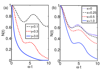
Figure 1: The negativity as function of $\omega t$ with (a) different $\gamma$’s ($\kappa=1$), and (b) different $\kappa$’s ($\gamma=0.3$) obtained by an average over $1000$ trajectories. The initial state is chosen as $(1/\sqrt{2})(|1\rangle_{A}|1\rangle_{B}+|0\rangle_{A}|0\rangle_{B})$.

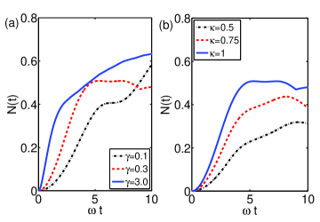
Figure 2: The negativity as function of $\omega t$ with (a) different $\gamma$’s ($\kappa=1$), and (b) different $\kappa$’s ($\gamma=0.3$) obtained by an average over $1000$ trajectories. The initial state is chosen as $|2\rangle_{A}|0\rangle_{B}$.

Entanglement dynamics of the qubit-qubit system in Markov and non-Markovian baths has been extensively studied in the last decade [30, 31, 32, 33, 34, 35, 36, 37, 38, 39, 40]. Equipped with the exact QSD equation for the qubit-qutrit system, we are in the position to study rigorously the non-Markovian entanglement and decoherence dynamics for this hybrid system. For the purpose of entanglement dynamics, qubit-qubit ($2\otimes 2$) and qubit-qutrit ($2\otimes 3$) systems are particularly interesting due to the fact that entanglement measured negativity [41, 42, 43, 44] serves both sufficient and necessary conditions for an arbitrary state of these two bipartite systems. Precisely, the negativity is defined as $N(\rho)\equiv||\rho^{T_{B}}||-1=2\sum_{j}|\mu_{j}|$, where $T_{B}$ stands for the partial transpose with respect to one of subsystems $B$, and $\mu_{j}$’s are the negative eigenvalues of the matrix $\rho^{T_{B}}$. A qubit-qutrit state represented by the density matrix $\rho$ is entangled if and only if $N(\rho)$ is positive. The negativity $N(\rho)$ varies from zero for all separable states to unity for the maximally entangled states. For a general pure state of qubit-qubit and qubit-qutrit system, it reduces to the definition of Wootters’ concurrence and generalized concurrence for pure states [45, 46], respectively.

Once the correlation function $\alpha(t,s)$ is chosen, it is straightforward to calculate these coefficient functions in eq. (21). In the following, for the sake of simplicity, we consider a Gaussian complex noise $z_{t}$ satisfying the Ornstein-Uhlenbeck process: $\alpha(t,s)=\frac{\Gamma\gamma}{2}e^{-\gamma|t-s|}$, where $\Gamma$ is the dissipation rate and $\gamma$ describes the memory time of the environment. More precisely, $\gamma^{-1}$ defines the finite correction time of the environment. When $\gamma\rightarrow\infty$, the correlation function approaches the Markov limit: $\alpha(t,s)=\Gamma\delta(t-s)$. In Appendix B, the details of the differential equations for all the functions $F_{j}$’s ($j=1,\cdots,8$) and $P_{j}$’s ($j=9,\cdots,13$) are provided. It should be noted that the $P_{j}$ terms contain explicitly the history integral over complex Gaussian noise $z_{t}$. It is expected that they will be important in non-Markovian dynamics when $\gamma$ is not too large (far from Markov regimes).

In the following numerical simulations, we choose $\omega_{A}=\omega_{B}=\omega$, $\Gamma=1$ and the double integral term about $P_{13}$ containing noises is neglected to save the computer memory. It is easy to see that the higher orders are clearly less important in a weakly non-Markovian regime.

In figs. 1(a) and 1(b), the initial state is a maximal entangled state $|\psi(0)\rangle=(1/\sqrt{2})(|1\rangle_{A}|1\rangle_{B}+|0\rangle_{A}|0\rangle_{B})$. Fig. 1(a) shows the effect of $\gamma$ on the decay rates of the entanglement of the system. When $\gamma$ is as large as $3$, the dynamics is seen to be very close to the Markov limit. It shows the reservoir can quickly ruin the coherence of the initial state, which evolves into a separable state monotonously. When $\gamma=0.1$, the environment has a long memory time, so that the non-Markovian features become dominant, hence the negativity exhibits a strong fluctuation pattern and maintains a highly entangled state for a long time. When $\gamma=0.3$, it shows a moderate non-Markovian behavior. Fig. 1(b) illustrates how the anisotropic coupling parameter $\kappa$ affects the entanglement evolution. The asymmetrical coupling slows down the entanglement decay gradually as the parameter $\kappa$ becomes smaller and smaller. The extreme case is that $\kappa=0$, where one of the subsystems is completely decoupled from the influence of the environment.

Figure. 2(a) plots the entanglement generation of the separable state $|\psi(0)\rangle=|2\rangle_{A}|0\rangle_{B}$. If the qubit is not interacting with the qutrit, then the entanglement generation is purely due to the indirect interaction between the subsystems induced by the common bath and memory times. For this initially separable state, the larger $\gamma$ (near-Markov reservoir) leads to a faster transition from $|2\rangle$ to $|1\rangle$ compared to the smaller $\gamma$ (a stronger non-Markovian regime). Interestingly, the near-Markov reservoir in turn causes a quicker generation of entanglement with one excitation transition in a short time interval. For some initially separable states, the non-Markovian property may be essential in entanglement generation. In the case of $\gamma=0.1$, representing a highly non-Markovian regime, it clearly shows that the dynamics generates a higher degree of entanglement than that in the case of $\gamma=0.3$ after $\omega t\approx 9$. While fig. 2(b) describes the effect of different $\kappa$’s on the entanglement generation with the same $\gamma$. It is very interesting to see that the entangling power is highly sensitive to the coupling balance for the qubit and qutrit interacting with the common bath.

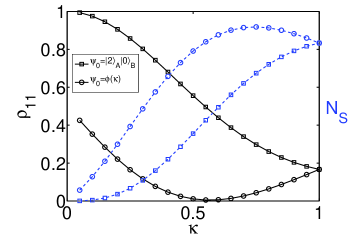
Figure 3: The distribution of the ground state $\rho_{11}$ (black solid lines) and the negativity of the steady state $N_{s}$ (blue dashed lines) as functions of $\kappa$ with different initial states in the long-time limit.

It is interesting to examine the long-time behavior of the combined qubit-qutrit system under the influence of the non-Markovian environment. For the Ornstein-Uhlenbeck noise, the information for the long-time limit may be obtained by solving the Markov master equation for the qubit-qutrit system

$$\partial_{t}\rho_{t}=-i[H_{\rm sys},\rho_{t}]+\frac{\Gamma}{2}[L,\rho_{t}L^{\dagger}]+\frac{\Gamma}{2}[L\rho_{t},L^{\dagger}].$$ (22)

Now we consider several interesting initial states in the four subspaces spanned by (i) $|2\rangle_{A}|1\rangle_{B}$, (ii) $|2\rangle_{A}|0\rangle_{B}$ and $|1\rangle_{A}|1\rangle_{B}$, (iii) $|1\rangle_{A}|0\rangle_{B}$ and $|0\rangle_{A}|1\rangle_{B}$, (iv) $|0\rangle_{A}|0\rangle_{B}$, respectively. When $\Gamma=1$, $\omega_{A}=\omega_{B}$, we have

$$\partial_{t}\rho_{66} = -(1+\kappa^{2})\rho_{66},$$

$$\partial_{t}\rho_{55} = \kappa^{2}\rho_{66}-\frac{\kappa}{2}(\rho_{45}+\rho_{54})-\rho_{55},$$

$$\partial_{t}\rho_{54} = \kappa\rho_{66}-\frac{\kappa}{2}(\rho_{44}+\rho_{55})-(1+\frac{\kappa^{2}}{2})\rho_{54},$$

$$\partial_{t}\rho_{44} = \rho_{66}-(1+\kappa^{2})\rho_{44}-\frac{\kappa}{2}(\rho_{54}+\rho_{45}),$$

$$\partial_{t}\rho_{33} = \rho_{55}-\rho_{33}-\frac{\kappa}{2}(\rho_{23}+\rho_{32})+\kappa(\rho_{45}+\rho_{54})+\kappa^{2}\rho_{44},$$

$$\partial_{t}\rho_{32} = \rho_{54}-(\frac{1}{2}+\frac{\kappa^{2}}{2})\rho_{32}-\frac{\kappa}{2}(\rho_{22}+\rho_{33})+\kappa\rho_{44},$$

$$\partial_{t}\rho_{22} = \rho_{44}-\frac{\kappa}{2}(\rho_{32}+\rho_{23})-\kappa^{2}\rho_{22},$$

$$\partial_{t}\rho_{11} = \rho_{33}+\kappa(\rho_{23}+\rho_{32})+\kappa^{2}\rho_{22},$$

where the notations for the six basis vectors are $|6\rangle=|2\rangle_{A}|1\rangle_{B}$, $|5\rangle=|2\rangle_{A}|0\rangle_{B}$, $|4\rangle=|1\rangle_{A}|1\rangle_{B}$, $||3\rangle=|1\rangle_{A}|0\rangle_{B}$, $|2\rangle=|0\rangle_{A}|1\rangle_{B}$, and $|1\rangle=|0\rangle_{A}|0\rangle_{B}$. From the above equations, one can easily conclude that for the stationary solutions we always have $\rho_{66}=\rho_{55}=\rho_{54}=\rho_{44}=0$ (they are independent on the initial states). But $\rho_{33}=-\kappa\rho_{32}$, $\rho_{22}=-\rho_{32}/\kappa$, $\rho_{11}=1-\rho_{33}-\rho_{22}$, which are dependent on the initial states. Therefore, we have

$$\rho_{t=\infty} = \rho_{11}(\infty)|00\rangle_{AB}\langle 00|$$ (23)

$$+ [1-\rho_{11}(\infty)]|\psi(\kappa)\rangle\langle\psi(\kappa)|,$$

where $|\psi(\kappa)\rangle=(1/\sqrt{1+\kappa^{2}})(\kappa|1\rangle_{A}|0\rangle_{B}-|0\rangle_{A}|1\rangle_{B})$, which is an eigenstate of the Lindblad operator $L=S_{-}^{A}+\kappa S_{-}^{B}$.

The final value of $\rho_{11}$ is a function of the $\kappa$ and the initial states as well as the negativity of the final state. The black-solid line with the square marker in Fig. (3) describes the probability distribution $\rho_{11}$ of the ground state $|0\rangle_{A}|0\rangle_{B}$ for the initial state $|\psi(0)\rangle=|2\rangle_{A}|0\rangle_{B}$. In the range $0<\kappa\leqslant 1$, it decreases with $\kappa$ monotonously. And the negativity [equals to $2(1-\rho_{11})\kappa/(1+\kappa^{2})$] is shown by the blue-dashed line with the same marker. It coincides with the curves in Fig. 2(b). We also plot the numerical results (the two lines with the circle marker) for the initial state $|\phi(\kappa)\rangle=(1/\sqrt{1+\kappa^{2}})(\kappa|2\rangle_{A}|0\rangle_{B}-|1\rangle_{A}|1\rangle_{B})$, which is also an eigenstate of $L$, but this one is not protected by the common dissipative environment. It shows clearly that the state evolves into a mixture of the ground state $|0\rangle_{A}|0\rangle_{B}$ and $|\psi(\kappa)\rangle$ given by (23). An interesting result arising from the above discussions is that the residue entanglement degree reaches its maximal value at $\kappa\approx 0.75$ instead of $1$ which corresponds to the balanced coupling. It is also interesting to see that the final state could become an approximate pure state when $\kappa\approx 0.55$, which demonstrates a rather different patterns from those initially separable states considered in this section.

4 Conclusion

In summery, we have investigated non-Markovian QSD approach to the qubit-qutrit system coupled to a zero-temperature bath. With the non-Markovian QSD equation, the entanglement dynamics of the qubit-qutrit system is studied carefully. The numerical simulations have been used to show the negativity dynamics for different initial states. We also discuss the long-time behaviors of the initially entangled or separable states of the hybrid system. Entanglement generation and decoherence have been shown to be sensitively dependent on coupling strength, memory time and initial states. The approach described here provides a fundamental tool for qubit-qutrit systems when the non-Markovian properties become important.

5 Appendix A: Equations of the Motions for the Coefficients and Boundary Conditions - General Case

By the time evolution equation for O-operator in eq. (19), we get a set of partial differential equations about the coefficient functions in eq. (18):

$$\partial_{t}f_{1}(t,s) = i(2\omega_{A}-\omega_{B})f_{1}+F_{1}f_{3}+F_{4}f_{1}+\kappa F_{4}f_{3}$$ (A1)

$$- \kappa F_{5}f_{4}-\kappa F_{8}f_{1}-\kappa P_{10}(t,s),$$

$$\partial_{t}f_{2}(t,s)=i\omega_{A}f_{2}+F_{2}f_{2}-F_{1}f_{6}-F_{3}f_{2}-\kappa F_{4}f_{6}$$

$$+\kappa F_{6}f_{2}-\kappa F_{7}f_{2}-P_{9}(t,s)-\kappa P_{11}(t,s),$$ (A2)

$$\partial_{t}f_{3}(t,s) = i\omega_{A}f_{3}+F_{3}f_{3}-\kappa F_{5}f_{7}+F_{7}f_{1}+\kappa F_{7}f_{3}$$ (A3)

$$- \kappa F_{8}f_{3}-\kappa P_{12}(t,s),$$

$$\partial_{t}f_{4}(t,s) = i\omega_{A}f_{4}+F_{1}f_{7}+F_{4}f_{4}+F_{4}f_{7}-F_{5}f_{4}$$ (A4)

$$- F_{8}f_{1}-P_{10}(t,s),$$

$$\partial_{t}f_{5}(t,s)=i\omega_{A}f_{5}+F_{5}f_{5}+\kappa F_{5}f_{8},$$ (A5)

$$\partial_{t}f_{6}(t,s) = i\omega_{B}f_{6}+F_{2}f_{6}-F_{4}f_{6}+\kappa F_{6}f_{6}$$ (A6)

$$- F_{7}f_{2}-P_{11}(t,s),$$

$$\partial_{t}f_{7}(t,s) = i\omega_{B}f_{7}+F_{3}f_{7}-F_{5}f_{7}+F_{7}f_{4}+\kappa F_{7}f_{7}$$ (A7)

$$- F_{8}f_{3}-P_{12}(t,s),$$

$$\partial_{t}f_{8}(t,s)=i\omega_{B}f_{8}+F_{8}f_{5}+\kappa F_{8}f_{8},$$ (A8)

$$\partial_{t}p_{9}(t,s,s_{1})=2i\omega_{A}p_{9}+F_{2}p_{9}-\kappa F_{5}p_{11}+\kappa F_{6}p_{9}$$

$$-\kappa F_{8}p_{9}+P_{9}f_{3}-\kappa P_{10}f_{6}+P_{11}f_{1}$$

$$+\kappa P_{11}f_{3}-\kappa P_{12}f_{2}-2\kappa P_{13}(t,s,s_{1}),$$ (A9)

$$\partial_{t}p_{10}(t,s,s_{1}) = 2i\omega_{A}p_{10}+F_{1}p_{12}+F_{4}p_{10}+\kappa F_{4}p_{12}$$ (A10)

$$+ P_{10}f_{5}+\kappa P_{10}f_{8},$$

$$\partial_{t}p_{11}(t,s,s_{1}) = i(\omega_{A}+\omega_{B})p_{11}+F_{2}p_{11}-F_{5}p_{11}$$ (A11)

$$+ \kappa F_{6}p_{11}-F_{8}p_{9}+P_{9}f_{7}-P_{10}f_{6}+P_{11}f_{4}$$

$$+ \kappa P_{11}f_{7}-P_{12}f_{2}-2P_{13}(t,s,s_{1}),$$

$$\partial_{t}p_{12}(t,s,s_{1}) = i(\omega_{A}+\omega_{B})p_{12}+F_{3}p_{12}+F_{7}p_{10}$$ (A12)

$$+ \kappa F_{7}p_{12}+P_{12}f_{5}+\kappa P_{12}f_{8},$$

$$\partial_{t}p_{13}(t,s,s_{1},s_{2}) = i(2\omega_{A}+\omega_{B})p_{13}+F_{2}p_{13}+\kappa F_{6}p_{13}$$ (A13)

$$+ P_{9}p_{12}+P_{11}p_{10}+\kappa P_{11}p_{12}+P_{13}f_{5}$$

$$+ \kappa P_{13}f_{8},$$

where $F_{j}=F_{j}(t)\equiv\int_{0}^{t}\alpha(t,s)f_{j}(t,s)ds$, $j=1,\cdots,8$; $P_{j}=P_{j}(t,s_{1})\equiv\int_{0}^{t}\alpha(t,s)p(t,s,s_{1})ds$, $j=9,\cdots,12$; $P_{13}=P_{13}(t,s_{1},s_{2})\equiv\int_{0}^{t}\alpha(t,s)p_{13}(t,s,s_{1},s_{2})ds$. And the boundary conditions are:

$$p_{9}(t,s,t) = -\kappa f_{1}(t,s)+f_{2}(t,s)-f_{3}(t,s),$$

$$p_{10}(t,s,t) = \kappa f_{1}(t,s)+f_{4}(t,s)-f_{5}(t,s),$$

$$p_{11}(t,s,t) = \kappa f_{2}(t,s)-\kappa f_{4}(t,s)+f_{6}(t,s)-f_{7}(t,s),$$

$$p_{12}(t,s,t) = \kappa f_{3}(t,s)-\kappa f_{5}(t,s)+f_{7}(t,s)-f_{8}(t,s),$$

$$p_{13}(t,s,t,s_{1}) = 0.5[\kappa p_{9}(t,s,s_{1})-\kappa p_{10}(t,s,s_{1})$$ (A14)

$$+ p_{11}(t,s,s_{1})-p_{12}(t,s,s_{1})].$$

6 Appendix B: Equations of the Motion for the Coefficients: Ornstein-Uhlenbeck Noise

In the case of the Ornstein-Uhlenbeck process, by the definitions and the boundary conditions in eq. (A14), we get a set of closed differential equations for $F_{j}$’s ($j=1,\cdots,8$), $\bar{P}_{j}$’s ($j=9,\cdots,12$) and $\tilde{P}_{13}$:

$$\partial_{t}F_{1}(t) = (-\gamma+2i\omega_{A}-i\omega_{B})F_{1}+F_{1}F_{3}+F_{1}F_{4}$$ (B1)

$$- \kappa F_{1}F_{8}+\kappa F_{3}F_{4}-\kappa F_{4}F_{5}-\kappa\bar{P}_{10},$$

$$\partial_{t}F_{2}(t) = \frac{\Gamma\gamma}{2}+(-\gamma+i\omega_{A})F_{2}+F_{2}^{2}-F_{1}F_{6}-F_{2}F_{3}$$ (B2)

$$+ \kappa F_{2}F_{6}-\kappa F_{2}F_{7}-\kappa F_{4}F_{6}-\bar{P}_{9}-\kappa\bar{P}_{11},$$

$$\partial_{t}F_{3}(t) = \frac{\Gamma\gamma}{2}+(-\gamma+i\omega_{A})F_{3}+F_{1}F_{7}+F_{3}^{2}+\kappa F_{3}F_{7}$$ (B3)

$$- \kappa F_{3}F_{8}-\kappa F_{5}F_{7}-\kappa\bar{P}_{12},$$

$$\partial_{t}F_{4}(t) = \frac{\Gamma\gamma}{2}+(-\gamma+i\omega_{A})F_{4}+F_{1}F_{7}-F_{1}F_{8}+F_{4}^{2}$$ (B4)

$$- F_{4}F_{5}+F_{4}F_{7}-\bar{P}_{10},$$

$$\partial_{t}F_{5}(t)=\frac{\Gamma\gamma}{2}+(-\gamma+i\omega_{A})F_{5}+F_{5}^{2}+\kappa F_{5}F_{8},$$ (B5)

$$\partial_{t}F_{6}(t) = \frac{\kappa\Gamma\gamma}{2}+(-\gamma+i\omega_{B})F_{6}+F_{2}F_{6}-F_{2}F_{7}$$ (B6)

$$- F_{4}F_{6}+\kappa F_{6}^{2}-\bar{P}_{11},$$

$$\partial_{t}F_{7}(t) = \frac{\kappa\Gamma\gamma}{2}+(-\gamma+i\omega_{B})F_{7}+F_{3}F_{7}-F_{3}F_{8}$$ (B7)

$$+ F_{4}F_{7}-F_{5}F_{7}+\kappa F_{7}^{2}-\bar{P}_{12},$$

$$\partial_{t}F_{8}(t)=\frac{\kappa\Gamma\gamma}{2}+(-\gamma+i\omega_{B})F_{8}+F_{5}F_{8}+\kappa F_{8}^{2},$$ (B8)

$$\partial_{t}\bar{P}_{9} = (-2\gamma+2i\omega_{A})\bar{P}_{9}+\frac{\Gamma\gamma}{2}(-\kappa F_{1}+F_{2}-F_{3})+F_{1}\bar{P}_{11}$$ (B9)

$$+ F_{2}\bar{P}_{9}-\kappa F_{2}\bar{P}_{12}+F_{3}\bar{P}_{9}+\kappa F_{3}\bar{P}_{11}-\kappa F_{5}\bar{P}_{11}$$

$$+ \kappa F_{6}\bar{P}_{9}-\kappa F_{6}\bar{P}_{10}-\kappa F_{8}\bar{P}_{9}-2\kappa\tilde{P}_{13},$$

$$\partial_{t}\bar{P}_{10} = (-2\gamma+2i\omega_{A})\bar{P}_{10}+\frac{\Gamma\gamma}{2}(\kappa F_{1}+F_{4}-F_{5})+F_{1}\bar{P}_{12}$$ (B10)

$$+ F_{4}\bar{P}_{10}+\kappa F_{4}\bar{P}_{12}+F_{5}\bar{P}_{10}+\kappa F_{8}\bar{P}_{10},$$

$$\partial_{t}\bar{P}_{11} = (-2\gamma+i\omega_{A}+i\omega_{B})\bar{P}_{11}+\frac{\Gamma\gamma}{2}(\kappa F_{2}-\kappa F_{4}+F_{6}$$ (B11)

$$- F_{7})+F_{2}\bar{P}_{11}-F_{2}\bar{P}_{12}+F_{4}\bar{P}_{11}-F_{5}\bar{P}_{11}-F_{6}\bar{P}_{10}$$

$$+ \kappa F_{6}\bar{P}_{11}+F_{7}\bar{P}_{9}+\kappa F_{7}\bar{P}_{11}-F_{8}\bar{P}_{9}-2\tilde{P}_{13},$$

$$\partial_{t}\bar{P}_{12} = (-2\gamma+i\omega_{A}+i\omega_{B})\bar{P}_{12}+\frac{\Gamma\gamma}{2}(\kappa F_{3}-\kappa F_{5}+F_{7}$$ (B12)

$$- F_{8})+F_{3}\bar{P}_{12}+F_{5}\bar{P}_{12}+F_{7}\bar{P}_{10}$$

$$+ \kappa F_{7}\bar{P}_{12}+\kappa F_{8}\bar{P}_{12},$$

$$\partial_{t}\tilde{P}_{13} = (-3\gamma+2i\omega_{A}+i\omega_{B})\tilde{P}_{13}+\frac{\Gamma\gamma}{4}(\kappa\bar{P}_{9}-\kappa\bar{P}_{10}$$ (B13)

$$+ \bar{P}_{11}-\bar{P}_{12})+F_{2}\tilde{P}_{13}+F_{5}\tilde{P}_{13}+\kappa F_{6}\tilde{P}_{13}$$

$$+ \bar{P_{9}}\bar{P}_{12}+\kappa F_{8}\tilde{P}_{13}+\bar{P}_{10}\bar{P}_{11}+\kappa\bar{P}_{11}\bar{P}_{12},$$

where $\bar{P}_{j}=\bar{P}_{j}(t)\equiv\int_{0}^{t}\alpha(t,s)P_{i}(t,s)ds$, $j=9,\cdots,12$; $\tilde{P}_{13}=\int_{0}^{t}\int_{0}^{t}\alpha(t,s_{1})\alpha(t,s)P_{13}(t,s,s_{1})dsds_{1}$; And the initial conditions for $F_{j}(0),j=1,\cdots,8$, $\bar{P}_{j}(0),j=9,\cdots,12$ and $\tilde{P}_{13}(0)$ are all zero.

References

- [1] Nielsen M. and Chuang I., Quantum Computation and Quantum Information, (Cambridge University Press, 2000).
- [2] Orszag M., Quantum Optics: Including Noise Reduction, Trapped Ions, Quantum Trajectories, and Decoherence, (2nd edition, Springer-Verlag, 2007).
- [3] Gardiner C. W., Zoller P., Quantum Noise, (Springer-Verlag, 2004).
- [4] Dalibard J., Castin Y., and Mølmer K., Phys. Rev. Lett. 68 (1992) 580.
- [5] Gardiner C. W., Parkins A. S., and Zoller P., Phys. Rev. A 46 (1992) 4363.
- [6] Carmicheal H. J., An Open System Approach to Quantum Optics, (Springer-Verlag, 1993).
- [7] Gisin N. and Percival I. C., J. Phys. A 25 (1992) 5677; J. Phys. A 26 (1993) 2233.
- [8] Breuer H. P. and Petruccione F., The Theory of Open Quantum Systems (Oxford University Press, USA, 2002).
- [9] Anastopoulos C., Hu B. L., Phys. Rev. A 62 (2000) 033821; Fleming C. H., Cummings N. I., Anastopoulos C., Hu B. L., arXiv:1012.5067v4.
- [10] Paz J. P., Roncaglia A. J., Phys. Rev. Lett. 100 (2008) 220401.
- [11] Piilo J., Maniscalco S., Härkönen K., and Suominen K. -A., Phys. Rev. Lett. 100 (2008) 180402.
- [12] An J. H., Zhang W. M., Phys. Rev. A 76 (2007) 042127; Tu M. W. Y., Zhang W. M., Phys. Rev. B 78 (2008) 235311.
- [13] Diósi L. and Strunz W. T., Phys. Lett. A 235 (1997) 569.
- [14] Diósi L., Gisin N., and Strunz W. T., Phys. Rev. A 58 (1998) 1699.
- [15] Strunz W. T., Diósi L., and Gisin N., Phys. Rev. Lett. 82 (1999) 1801.
- [16] Yu T., Diósi L., Gisin N., and Strunz W. T., Phys. Rev. A 60 (1999) 91; Phys. Lett. A 265 (1999) 331.
- [17] Strunz W. T., Chem. Phys. 268 (2001) 237.
- [18] Gambetta J., Wiseman H. M., Phys. Rev. A 66 (2002) 012108; Phys. Rev. A 68 (2003) 062104.
- [19] Strunz W. T. and Yu T., Phys. Rev. A 69 (2004) 052115.
- [20] Yu T., Phys. Rev. A 69 (2004) 062107.
- [21] Alonso D., de Vega I., Phys. Rev. Lett. 94 (2005) 200403.
- [22] Bassi A. and Ferialdi L., Phys. Rev. Lett. 103 (2009) 050403.
- [23] Jing J., Zhao X. Y., You J. Q., Yu T., arXiv:1012.0364.
- [24] Roden J., Eisfeld A., Wolff W. and Strunz W. T., Phys. Rev. Lett. 103 (2009) 058301.
- [25] Khan M. H. A., Perkowski M. A., J. Sys. Arch. 53 (2007) 453.
- [26] Checinska A., Wodkiewicz K., Phys. Rev. A 76 (2007) 052306.
- [27] Jing J., Yu T., Phys. Rev. Lett. 105 (2010) 240403.
- [28] Ann K., Jaeger G., Phys. Lett. A 372 (2008) 579.
- [29] Zhao X. Y., Jing. J, Corn B., Yu T. Phys. Rev. A 84 (2011) 032101.
- [30] Rajagopal A. K. and Rendell R. W., Phys. Rev. A 63 (2001) 022116; Zyczkowski K., Horodecki P., Horodecki M. and Horodecki R., Phys. Rev. A 65 (2001) 012101; Daffer S., Wodkiewicz K. and McIver J. K., Phys. Rev. A 67 (2003) 062312; Diósi L, in Irreversible Quantum Dynamics, edited by Benatti F. and Floreanini R. (Springer, Berlin, 2003), pp. 157-163.
- [31] Yu T. and Eberly J. H., Phys. Rev. B 66, 193306 (2002); Phys. Rev. A 68 (2003) 165322.
- [32] Yu T., Eberly J. H., Phys. Rev. Lett. 93, 140404 (2004); Yu T., Eberly J. H., Science 323 (2009) 598.
- [33] Carvalho A. R. R., Mintert F., and Buchleitner A., Phys. Rev. Lett. 93 (2004) 230501.
- [34] Bellomo B., Lo Franco R., and Compagno G., Phys. Rev. Lett. 99 (2007) 160502.
- [35] Maniscalco S., and Petruccione F., Phys. Rev. A 73 (2006) 012111.
- [36] Ficek Z., Tanas R., Phys. Rev. A 74 (2006) 024304; Natali S., Ficek Z., Phys. Rev. A 75 (2007) 042307; Ficek Z., Front. Phys. China, 5 (1) (2010) 29 and references therein.
- [37] Huang J. H., Wang L. G., Zhu S. Y., Phys. Rev. A 81 (2010) 064304.
- [38] Sun Z., Wang X. -G., and Sun C. P., Phys. Rev. A 75 (2007) 062312.
- [39] Helm J. and Strunz W. T., Phys. Rev. A 80 (2009) 042108.
- [40] Yu T., Eberly J. H., Opt. Commun. 283 (2010) 676.
- [41] Peres A., Phys. Rev. Lett. 77 (1996) 1413.
- [42] Horodecki M., Horodecki P., Horodecki R., Phys. Lett. A 223 (1996) 1.
- [43] Vidal G. and Werner R. F., Phys. Rev. A 65 (2002) 032314 .
- [44] Horodecki R., Horodecki P., Horodecki M., and Horodecki K., Rev. Mod. Phys. 81 (2009) 685.
- [45] Wootters W. K., Phys. Rev. Lett. 80 (1998) 2245.
- [46] Ou Y. C., Fan H., and Fei S. M., Phys. Rev. A 78 (2008) 012311.