Decorrelation Times of Photospheric Fields and Flows

Abstract

We use autocorrelation to investigate evolution in flow fields inferred by applying Fourier Local Correlation Tracking (FLCT) to a sequence of high-resolution (0.3 ″), high-cadence ($\simeq 2$ min) line-of-sight magnetograms of NOAA active region (AR) 10930 recorded by the Narrowband Filter Imager (NFI) of the Solar Optical Telescope (SOT) aboard the Hinode satellite over 12–13 December 2006. To baseline the timescales of flow evolution, we also autocorrelated the magnetograms, at several spatial binnings, to characterize the lifetimes of active region magnetic structures versus spatial scale. Autocorrelation of flow maps can be used to optimize tracking parameters, to understand tracking algorithms’ susceptibility to noise, and to estimate flow lifetimes. Tracking parameters varied include: time interval $\Delta t$ between magnetogram pairs tracked, spatial binning applied to the magnetograms, and windowing parameter $\sigma$ used in FLCT. Flow structures vary over a range of spatial and temporal scales (including unresolved scales), so tracked flows represent a local average of the flow over a particular range of space and time. We define flow lifetime to be the flow decorrelation time, $\tau$. For $\Delta t>\tau$, tracking results represent the average velocity over one or more flow lifetimes. We analyze lifetimes of flow components, divergences, and curls as functions of magnetic field strength and spatial scale. We find a significant trend of increasing lifetimes of flow components, divergences, and curls with field strength, consistent with Lorentz forces partially governing flows in the active photosphere, as well as strong trends of increasing flow lifetime and decreasing magnitudes with increases in both spatial scale and $\Delta t$.

1 Introduction

Estimates of photospheric velocities can be combined with the ideal Ohm’s law to determine the fluxes of magnetic energy and helicity across the photosphere (e.g., Chae 2001; Démoulin and Berger 2003; Schuck 2006). These fluxes probably play important roles in driving the corona to flare (Welsch et al., 2009) and to launch coronal mass ejections (CMEs), as well as coronal heating (Tan et al., 2007). Several techniques can be used to estimate photospheric flows, including tracking methods (e.g., Fisher and Welsch 2008; Schuck 2006), balltracking (Potts et al., 2004) and feature tracking (DeForest et al., 2007). Techniques for estimating photospheric velocities, however, are imperfect (Rieutord et al., 2001; Welsch et al., 2007; Schuck, 2008), so efforts to improve estimation techniques are ongoing.

Autocorrelation of image sequences has been used to quantify evolutionary timescales of structures in the solar atmosphere. In this approach, a measure of correlation (e.g., linear or rank-order correlation) is computed between pixel values at some initial time $t_{i}$ and the corresponding pixel values at a later time $t_{i}+\Delta T$, where we refer to $\Delta T$ as the lag time. As image features evolve with increasing $\Delta T$, measures of correlation computed this way typically drop. For instance, Tritschler et al. (2007) investigated internetwork and network fine structure of the quiet Sun at disk center in the Ca II K line. Welsch et al. (2009) autocorrelated 96-minute-cadence, line-of-sight (LOS) magnetograms of a few dozen active regions imaged by the MDI instrument (Scherrer et al., 1995) in full-disk mode (with $\simeq 2\arcsec$ pixels) over lag times ranging from the data’s nominal 96-minute cadence to several days. They found decorrelation times for the magnetic field, defined as a drop in the autocorrelation to $1/e\sim 0.37$, on the order of $72$ hours, with considerable variation between active regions. Welsch et al. (2009) also estimated horizontal flows in their active region sample by applying tracking methods to pairs of magnetograms separated in time by a tracking interval, $\Delta t$, equal to the data’s 96-minute cadence. The flows were independently estimated by using two distinct methods, Fourier local correlation tracking (FLCT; Fisher and Welsch 2008) and the differential affine velocity estimator (DAVE; Schuck 2006). Apodization windows of 8 and 9 pixels, respectively, were used, so motions on smaller scales were averaged away over the apodization window. By autocorrelating the $x$- and $y$-components of the estimated flows, they found flow lifetimes of two to three 96-minute steps on this $\sim 12$ Mm spatial scale.

The autocorrelation approach employed by Welsch et al. (2009) was useful for estimating the lifetime of magnetic field structures and flows on the particular spatial scales they studied. But what are the lifetimes of magnetic and flow structures on different spatial scales? How do flow lifetimes vary as a function of length scale? And what are the lifetimes of flow properties, such as vortical or converging motions? From the general properties of turbulent flows like those operating at the solar photosphere, we expect structure in flow fields to be present over a range of spatial scales, with a range of lifetimes.

Further, little effort has been undertaken to understand how variations in tracking cadence $\Delta t$, noise, and choice apodization window size affect flow inference. How do variations in these quantities influence estimated flows? Abramenko et al. (2011) used feature tracking to follow bright points over a range of $\Delta t$’s, and characterized their motion as super-diffusive. The average speeds implied by their diffusive model decreased with increasing $\Delta t$. Chae et al. (2000) applied an LCT algorithm to chromospheric H-$\alpha$ images, and noted that $\Delta t$ must be long enough for displacements to be large enough to be detected by LCT, but not so long that displacements are larger than the apodization window. They also found that choosing window sizes that were too small increased random velocities due to noise. Chae et al. (2004) found slower average speeds for longer $\Delta t$’s. More recently, Verma and Denker (2011) conducted an investigation of the effects of parameter selection on flows inferred by applying local correlation tracking (LCT) to high-cadence, high-resolution (0.11 ″pixel scale) G-band images of a field of view containing sunspot umbrae, penumbrae, and quiet-Sun regions, observed by the broadband filter imager (BFI) of the SOT (Tsuneta et al., 2008) aboard the Hinode satellite (Kosugi et al., 2007). The evolutionary time scales and spatial scales of the underlying image structures motivated their selection of tracking intervals between 15 and 200 s, and apodization windows of 600 – 2400 km. They found decreases in flow speeds both as the apodization window size increased, and as flow maps were averaged over longer time periods. Because photospheric magnetic flux is long-lived, tracking methods can be applied to magnetograms separated in time by much larger tracking intervals — e.g., longer than an hour, as done by Welsch et al. (2009).

Here, we address these and other topics by using FLCT to track a nearly 13-hour sequence of high-resolution ($0.16\arcsec$ pixels, with a $\sim 0.32\arcsec$ diffraction limit), rapid cadence ($\simeq 2$ min) LOS magnetograms of NOAA AR 10930, recorded by the SOT/NFI (Tsuneta et al., 2008; Suematsu et al., 2008; Ichimoto et al., 2008; Shimizu et al., 2008) instrument aboard Hinode over 2006 December 12 – 13. This active region was the source of an X-class flare and CME during our tracking interval: the flare began around 13-Dec-2006 02:15UT and peaked around 02:40 UT in GOES 1–8 Å  X-rays.Tan et al. (2009) also investigated flows in this active region, focusing on the relationship of penumbral flows and evolution to the flare, and Schrijver et al. (2008) conducted a comparative study of coronal magnetic field extrapolations derived from vector magnetograms of this active region.

This paper’s primary goals are: first, to investigate the effects of choices of tracking parameters on inferred flows; and second, to characterize the lifetimes and other properties of flows as functions of spatial scale and magnetic field. We begin by describing the magnetogram dataset in more detail (§2), then describe the methods we used to estimate flows (§3), present our analysis of the lifetimes of fields (§4) and flows (§5), and conclude with a brief summary of our results and their implications (§6).

2 Hinode SOT/NFI Magnetograms

We studied a sequence of Hinode SOT/NFI Fe I 6302 Åshuttered magnetograms of AR 10930 with $0.16\arcsec$ pixels, created from the Stokes $V/I$ ratio in Level 0 data, recorded between 12-Dec-2006 at 14:00 and 13-Dec-2006 at 02:58. The USAF/NOAA Solar Region Summary issued at 24:00 UT on 12-Dec-2006 listed AR 10930 at S06W21, meaning it was near disk center during this interval. At this wavelength, the diffraction limit of the Solar Optical Telescope’s 50 cm aperture is $1.22\lambda/a\simeq 0.32\arcsec$. We show initial and final magnetograms from the sequence in Figure 1. At that stage of the Hinode mission, a bubble present within the NFI instrument degraded image quality in part of the field of view. In these frames, the affected pixels are in an area between from about 300 – 900 in $x$ and above about $900$ in $y$. To account for the bubble, we exclude pixels above $y=848$ in all our analyses of flow properties and lifetimes (although this region is retained in some images shown in this paper).

To convert the measured Stokes $I$ and $V$ signals into pixel-averaged flux densities, we applied the approximate calibration used by Isobe et al. (2007),

$$B_{\rm LOS}=-\frac{C_{V}}{0.798C_{I}}\times 10000~{}~{}({\rm Mx\,cm}^{-2})~{},$$ (1)

where $B_{\rm LOS}$ is the estimated LOS flux density, $C_{I}$ and $C_{V}$ are counts in the $I$ and $V$ images, respectively, and $C_{V}/0.798$ gives the circular polarization. As noted by Isobe et al. (2007), this linear scaling is only approximate. In particular, in the dark cores of umbrae, the decrease in $I$ introduces nonlinearity into the $V/I$ ratio. This effect can produce spurious weak field regions in umbrae. A more complex, nonlinear calibration would be required to overcome this artifact. Since our primary goal is to investigate the time evolution of structure in this magnetogram sequence, we have not pursued efforts to correct such artifacts in the $V/I$ magnetograms.

A detailed spectroscopic analysis of fields in this active region using Hinode SpectroPolarimeter (SP; Tsuneta et al. 2008) data was undertaken by Schrijver et al. (2008), who created one vector magnetogram with approximately 0.63 ″pixels near the middle of our tracking interval, around 21:00 UT.Reprojection employed in their reduction procedure limits the ability to directly apply those results with our magnetogram data set, but, as described in Appendix A, we manually co-registered and resampled this SP vector magnetogram to map vertical magnetic field $B_{z}$ and field strength $|{\mathbf{B}}|$ from this magnetogram onto the $(4\times 4)$-binned NFI magnetogram closest to the midpoint of the 45-minute SP scan (at 21:52 UT).

The AR was at about S06W21 toward the end of our observations, and NFI’s field of view (FOV) subtends about 10 heliocentric degrees at disk center. These facts imply cosines between the line of sight and the local vertical direction within the AR ranging from 0.88 to 0.96, corresponding to variations in pixel scales from foreshortening of a few percent across the FOV. Over the earlier part of magnetogram sequence, upon which much of our analysis is focused, these variations are slightly smaller. Consequently, we take these modest distortions as acceptable, and opt not to reproject the magnetograms prior to tracking. Reprojection is, however, certainly appropriate for tracking studies over much larger fields of view, e.g., that of Welsch et al. (2009), who estimated velocities simultaneously across fields of view out to 45^∘ from disk center.

Apart from three abnormally large time steps of approximately 600 s each, and two relatively small time steps of 26 s each, the 380 frames we analyze have a cadence of 121.4 $\pm$ 1.2 s.

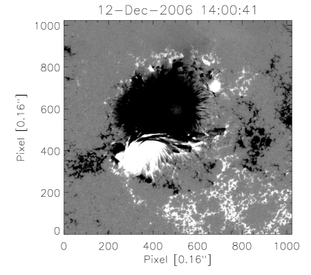
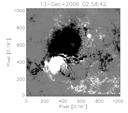
Figure 1: Left: Initial Hinode/NFI LOS magnetogram (white is positive flux, black is negative) from the 13-hour data sequence we investigated, at full resolution (0.16 ″pixels) with the saturation level set at $\pm 500$ Mx cm^-2. Right: Final magnetogram in the sequence.

To study frame-to-frame changes in the magnetic field, we must first remove artificial evolution due to whole-image shifts (rigid motion of each image) between frames, due primarily to variations in spacecraft pointing. To accomplish this, we first determined the frame-to-frame shift between the central regions of each pair of images (cropping the outer 10% of pixels along each edge), using FFTs to compute the frame-to-frame cross correlation function and a second-order Taylor series approximation to estimate the displacement vector of the function’s peak, to sub-pixel accuracy (Fisher and Welsch, 2008). We then used Fourier interpolation to estimate pixel values implied by a shift of the negative of the cumulative displacement from the initial frame in the sequence. Any wrapped pixels arising from this shift, due to the assumed periodicity, were then zeroed (as may be seen in a thin strip along the bottom of the right panel of Figure 1). In Figure 2, we show the cumulative shifts in $x$ and $y$ over the duration of the magnetogram sequence. Large shifts in image alignment occur with an approximate periodicity similar to that of Hinode’s 98-minute orbital period. (Katsukawa et al., 2010).

In Figure 2, we also show the total unsigned flux and negative of the net flux (there is more negative LOS flux than positive; but the right plot axis is positive, so we changed the sign of the net flux), which both exhibit periodicities on a timescale similar to that of the whole-frame shifts. Analysis of Fourier spectra of the time series in pixels (not shown) shows a significant excess power near the orbital frequency, but little evidence of helioseismic P-mode leakage into the magnetogram signal. Given the large Doppler shift from orbital motion, observed periodicities could arise from leakage of Doppler shifts induced by spacecraft orbital motion into the Stokes $V$ measurement. Thermal variations in the instrument might also be responsible.

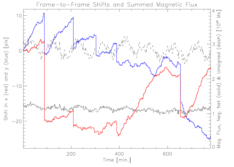
Figure 2: Left axis: Cumulative frame-to-frame shifts (in pixels) in the $x$ (red) and $y$ (blue) directions between pairs of magnetograms in the NFI sequence that we analyzed, with respect to the initial magnetogram. Right axis: total unsigned flux (dashed) and the negative of net flux (solid). Variations in flux probably arise from crosstalk due to Doppler shifts induced by spacecraft orbital motion into the Stokes $V$ signal.

As discussed in more detail below, local fluctuations in field strength from noise can mimic changes from true magnetic evolution, implying estimated flows will be inaccurate in regions where the measured fields are near the magnetograph noise level. We estimated this noise level using the procedure of Hagenaar et al. (1999). First, we spatially binned the data $2\times 2$ to $0.32\arcsec$-wide pixels, to approximate the SOT diffraction limit of $0.3\arcsec$. Next, we created histograms of pixel values in each frame in the sequence, in bins of 3 Mx cm^-2. Then, assuming the core of the distribution in signals arises purely from noise, we fit a Gaussian, $\exp[-(B-B_{0})^{2}/(2a^{2})$, to the central region of the histogram, $\pm 10$ Mx cm^-2. Over the course of the tracking interval, fitted values of the width parameter $a$ for single magnetograms ranged from a high near 17 Mx cm^-2 at the start of the run to lows near 7 Mx cm^-2 toward the end of the run. For simplicity, we therefore take 15 Mx cm^-2 as a uniform estimate of the noise level.

3 Estimating Flows

Assuming magnetic diffusivity is negligibly small over the time interval $\Delta t$ between a pair of successive magnetograms, Démoulin and Berger (2003) argued that the apparent motion of magnetic flux from one magnetogram to the next over $\Delta t$ could be described by a “footpoint velocity” ${\mathbf{u}}$, that is related to the plasma velocity ${\mathbf{v}}$ by

$${\mathbf{u}}B_{n}={\mathbf{v}}B_{n}-v_{n}{\mathbf{B}}_{h}~{},$$ (2)

where $\,\hat{\mathbf{n}}$ denotes the unit vector normal to the surface, the $n$ subscript denotes the normal component of a vector, and the $h$ subscript denotes the horizontal components of a vector, which are perpendicular to $\,\hat{\mathbf{n}}$. This assumption can be used to express the normal component of the magnetic induction equation in terms of a continuity-like, finite-difference equation,

$$\frac{\Delta B_{n}}{\Delta t}+\nabla_{h}\cdot({\mathbf{u}}B_{n})=0~{},$$ (3)

where $\Delta B_{n}=B_{n}(t_{f})-B_{n}(t_{i})$ is the change in the normal magnetic field between the initial time $t_{i}$ and the final time $t_{f}$, and $\nabla_{h}$ is approximated with finite differences in the spatial coordinates orthogonal to the normal direction. The analogy with the continuity equation is not precise, because unlike number or mass densities, which are always positive, magnetic flux can be positive or negative. So, unlike total particle number or total mass in a volume, neither total signed nor total unsigned flux is conserved in a magnetogram: existing opposite polarity fluxes can cancel, or new bipolar flux can emerge.

Démoulin and Berger (2003) argued that tracking methods applied to magnetograms estimate ${\mathbf{u}}$, instead of ${\mathbf{v}}_{h}$ (cf., Chae 2001), but Schuck (2005, 2008) argued that some tracking methods return a biased estimate, $\tilde{\mathbf{u}}$, with the contribution from ${\mathbf{v}}_{h}$ weighted more heavily than in the true ${\mathbf{u}}.$ The term “footpoint velocity” implicitly refers to extensions of magnetic flux above the magnetogram surface. Welsch (2006) used the alternative “flux transport velocity” to refer to ${\mathbf{u}}$ without reference to field structure above or below the magnetogram. For purposes of tracking, we assume the LOS field, $B_{\ell}$, derived from the NFI observations, approximates the normal field $B_{n}$.

We used the FLCT code (Welsch et al., 2004; Fisher and Welsch, 2008) to estimate flux transport velocities for this dataset. The FLCT code uses Fourier cross-correlation of $B_{n}(t_{i})$ with $B_{n}(t_{f})$ near a given pixel, say one centered at $(x_{j},y_{k})$, to determine the two-component displacement $\Delta{\mathbf{R}}$ of magnetic field structure between the magnetograms near $(x_{j},y_{k})$; division by $\Delta t$ then results in a velocity estimate at $(x_{j},y_{k})$. The correlation is localized by first weighting each magnetogram by a Gaussian windowing function, $\exp(-r_{jk}^{2}/\sigma^{2})$, where $r_{jk}$ is distance from $(x_{j},y_{k})$, and $\sigma$ is a free parameter. Optionally, low-pass filtering, with a Gaussian roll-off, can be applied to the Fourier spectra prior to performing the cross-correlation. In tests applying shifts to quiet-Sun magnetograms, Fisher and Welsch (2008) found roll-off values of $0.2k_{\rm max}$ – $0.5k_{\rm max}$ improved recovery of the applied shifts, where $k_{\rm max}$ is the highest wavenumber each dimension. In this work, we used a roll-off wavenumber of 0.5 $k_{\rm max}$, which corresponds to relatively weak Fourier filtering.

Like FLCT, other tracking methods typically apply an apodization or windowing function, the spatial extent of which is a free parameter, to the initial and final magnetograms, and find a velocity that extremizes some functional over this window (Schuck, 2006). Given data with sufficient cadence, the interval $\Delta t$ between pairs of magnetograms to be tracked can also be varied. Tracking methods therefore estimate velocities from the effects of actual velocities averaged both spatially over the windowed region and temporally over the time interval $\Delta t$ between magnetograms. This averaging implies that flows on spatial scales smaller than the windowing function, and with lifetimes shorter than $\Delta t$, cannot be recovered in the flow estimation process.

Beyond these algorithmic aspects of the tracking process, it can be also seen that noise and other artifacts in magnetogram measurements will contribute to the difference $\Delta B_{n}$ in equation (3), implying such effects can influence estimated velocities.

These considerations motivate efforts to understand the interplay between windowing and tracking cadence and flow spatial scale and lifetime, as well as the effects of magnetogram noise. To investigate these relationships, we estimated flux transport velocities from pairs of magnetograms that were separated in time by eight varying intervals, with $\Delta t\in\{$2, 4, 8, 16, 32, 64, 128, 256$\}$ minutes, that were both unbinned and binned to six varying macropixel sizes $\Delta x\in\{$2, 4, 8, 16, 32, 64 $\}$ in terms of the data’s original $0.16\arcsec$ pixels, with four choices of apodization parameter $\sigma\in\{$2, 4, 8, 16 $\}$. Pixel values were simply averaged when rebinned, which does not exactly mimic how magnetographs with either worse spatial resolution or poor weak-field sensitivity would detect magnetic flux.

Since we are interested in characterizing the effects of noise on estimated flows, we tracked all pixels above a threshold of 15 Mx cm^-2, which is both near our estimate of the noise level, and includes the spurious weak-field regions in the sunspot cores.

4 Lifetimes of Magnetic Structures

To provide context for the time evolution of flows on varying spatial scales, we autocorrelated the magnetograms themselves, at several spatial resolutions: with $0.16\arcsec$ pixels, and then with data rebinned to macropixels $\Delta x\in\{2,4,8,16,32,64\}$ pixels on a side. While each magnetogram is a 2D array, we computed the correlations as if both were 1D arrays. All pixels outside of the bubble region were used, not just those above the noise threshold used for tracking. The colored curves in Figure 3 show rank-order correlation coefficients for the autocorrelations at each spatial resolution for increasing lag time. In addition, the black dashed and solid curves show frame-to-frame linear and rank-order correlations, respectively, for the $2\times 2$ binned data. Note the limited range of the $y$-axis.

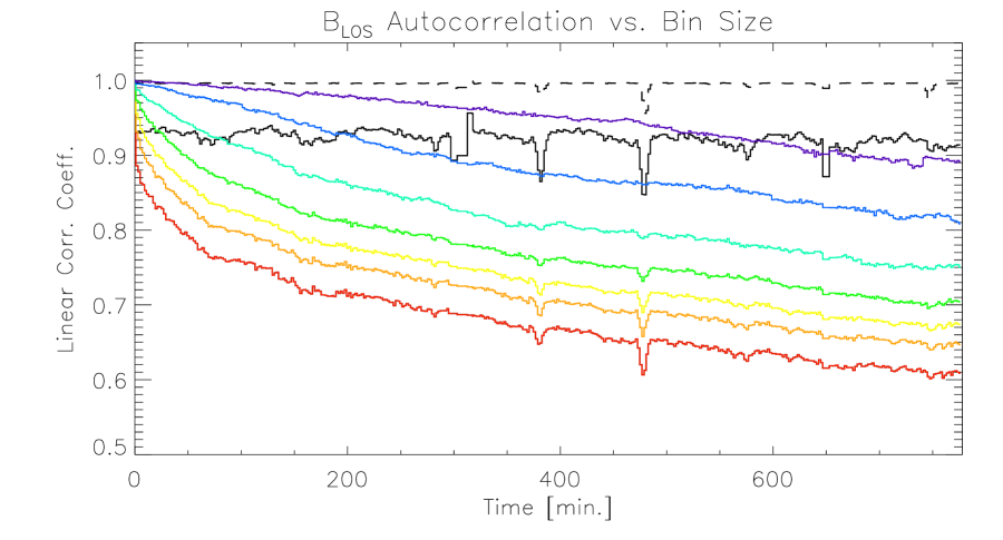
Figure 3: Colored curves show rank-order autocorrelation coefficients with increasing lag times, for magnetograms at several spatial binnings: red is for $0.16\arcsec$-pixel data; orange, yellow, green, aqua, blue, and purple are for data rebinned $2\times 2,4\times 4,8\times 8,16\times 16,32\times 32,$ and $64\times 64$, respectively. The black dashed and solid lines show frame-to-frame linear and rank-order correlation coefficients, respectively, for data binned $2\times 2$. Note the limited range of the vertical axis. Downward spikes before $500$ minutes arise from frames with many cosmic ray hits. The effects of the X-class flare can be seen as small blips near $743$ minutes.

The high frame-to-frame correlations imply that the magnetic field does not evolve much from one magnetogram to the next. It can also be seen that frame-to-frame linear correlations hover around unity, but frame-to-frame rank-order correlations are significantly lower, implying rank-order correlation is a more sensitive test of differences between magnetograms. This plot also shows that the lifetime of this active region’s magnetic structure, over the entire magnetogram field of view, is much longer than the duration of the dataset that we analyze.

Several artifacts are also present in these time series. Downward spikes in correlations correspond to frames in which isolated pixels contained large fluctuations, probably due to hits by cosmic rays. Despiking the magnetograms can remove these spikes, but here we are interested in the effects of such artifacts on autocorrelations. Larger binnings average out these effects. In terms of lag times plotted here, the start time of X-class flare that began around 02:28UT on 2006-Dec-13 corresponds to $743$ minutes, and its effects can be seen as small wiggles in some autocorrelation curves near the right end of the plot.

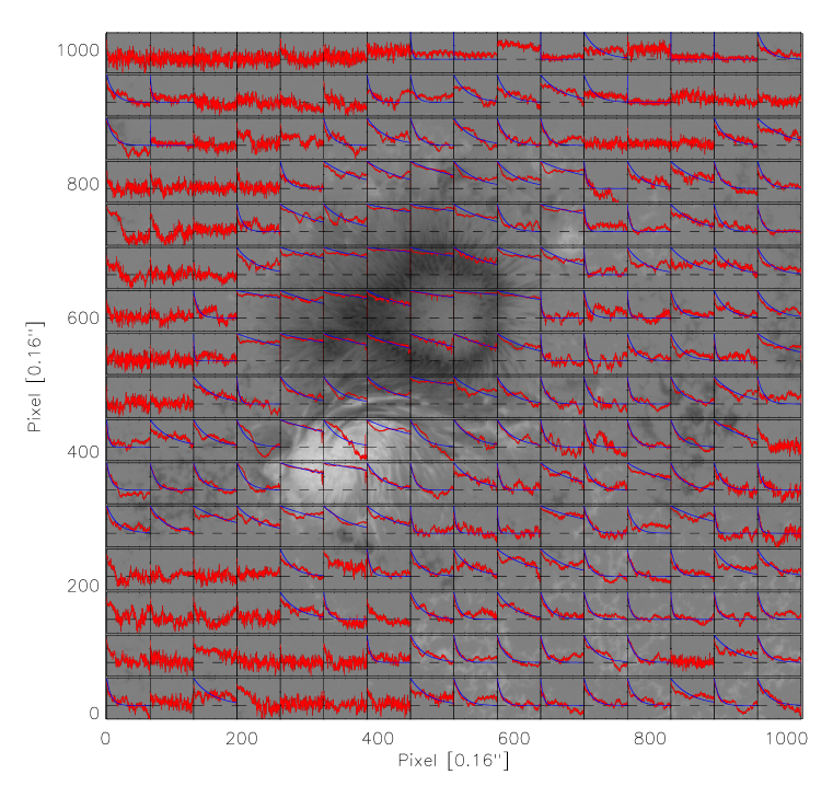
Figure 4: The grayscale image is $|B_{\rm LOS}|$ in a full-resolution magnetogram, with saturation at $\pm 4$ kG. Red curves show rank-order autocorrelations of $B_{\rm LOS}$, in $(32\times 32)$-binned subregions of ($2\times 2$)- binned data, vs. lag time, up to the duration of the dataset. The vertical range in each cell is [-0.5, 1.0], with a dashed black line at zero correlation. Blue curves show one-parameter fits to the decorrelation in each subregion, assuming exponential decay, with the decay constant as the only free parameter. Only subregions with median occupancy of at least 20% of pixels above our 15 G threshold were fit. As expected, field structures persist longer in stronger-field regions.

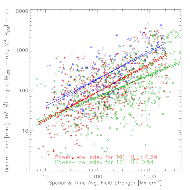
Figure 5: Fitted lifetimes of boxcar-averaged $|B_{\rm LOS}|$ and $|{\mathbf{B}}|$, averaged over each subregion, for the non-bubble region of the FOV. Blue triangles correspond to $(32\times 32)$-binned subregions (from fits in Figure 4) of $|B_{\rm LOS}|$. Red +’s correspond to $(16\times 16)$-binned subregions $|B_{\rm LOS}|$ (autocorrelations and fits at this resolution are not plotted in this paper), and green $\times$’s correspond to $|{\mathbf{B}}|$ averaged over $(16\times 16)2$-binned subregions. Fitted exponents to log-log values of $|B_{\rm LOS}|$ and $|{\mathbf{B}}|$ for $(16\times 16)$ bins are shown with corresponding colors. Dashed lines correspond to uncertainties in each fitted slope, based upon $\chi^{2}$; the slope of the blue fit (0.68) is similar to the red fit (0.69).

Distinct types of magnetic regions — notably, sunspots, plage, and quiet Sun — all influence the autocorrelations in Figure 3. By investigating the lifetimes of magnetic structures on smaller spatial scales, we can better understand the lifetimes of magnetic structures in each type of region. Accordingly, in Figure 4, we show autocorrelations (red curves) for $B_{\rm LOS}$ in $(32\times 32)$-binned subregions of ($2\times 2$)-binned data (so each subregion is $(64\times 64)$ full-resolution pixels). In the same figure, we also show one-parameter fits (blue curves) to the decorrelation in each subregion, assuming the autocorrelation function decays exponentially with lag time $\Delta T$, $\exp(-\Delta T/\tau)$, with the decay constant $\tau$ as the only free parameter. In each subregion, we take the fit decay constant, $\tau$, to be the lifetime of the structure in that subregion. We define the occupancy of a subregion to be the percentage of pixels above our 15 G noise threshold. Only pixels with a median occupancy, over the dataset’s duration, of at least 20% were fit. Background gray contours in the figure show 50 G and 200 G levels of $|B_{\rm LOS}|$ from the initial magnetogram (in full-resolution pixels), so variations in lifetimes can be understood in the context of active region structure.

We then investigated the dependence of magnetic lifetime on field strength. To start, we computed a measure of subregion field strength by boxcar averaging flux densities from $|B_{\rm LOS}|$ from the five initial magnetograms in our sequence at $(2\times 2)$ resolution, then taking the absolute value, then computing the spatial average of this unsigned, boxcar-averaged flux density over each subregion. We chose to use this measure of initial field strength to address the question: “For a given current field strength, how long will a structure persist?” The relatively short fitted lifetimes of some magnetic regions suggests that averaging over longer intervals — e.g., the length of the entire run — would imply averaging over several magnetic turnover times. It can be seen in Figure 4 that some of the fits represent the evolution poorly, but many fits match the observations well, given the single free parameter. Of the 195 subregions with at least 20% above-threshold occupancy, only four have fitted lifetimes that are less than the two-minute nominal cadence (see, e.g., the two subregions to the left of the top-right subregion). We ignore these too-short fits as pathological. In Figure 5, we plot the fitted lifetimes as a function of these spatially and temporally averaged subregion fields (blue +’s). A linear fit between the logarithms of each returns a power-law exponent of 0.66. The solid blue line shows the fit, while the dashed blue lines reflect uncertainty in the fitted slope, based upon $\chi^{2}$ computed from the fit. This trend is consistent with the idea that convection disrupts magnetic field structures, but stronger magnetic fields more strongly inhibit convection (Title et al., 1992; Berger et al., 1998; Welsch et al., 2009), so structures persist longer in stronger-field regions. Despite the trend of increasing lifetime with field strength, we note some high-field-strength regions have short lifetimes. Relatively rapid evolution in these high-field strength regions might play some role in flare activity, but pursuing this question is beyond the scope of this paper.

To investigate the dependence of this field-strength-versus-lifetime relationship on spatial scale, we repeated this procedure with the subregion size reduced to $16^{2}$ ($2\times 2$)-binned pixels (autocorrelations and fits at this resolution are not shown). Lifetimes as a function of subregion-averaged field strength are plotted in red in Figure 5, excluding 28 subregions with fitted lifetimes $<2$ min (of 733 subregions with at least 20% above-threshold occupancy). A linear fit between the logarithms of field strengths and lifetimes returns a power-law exponent of 0.69 in this case. The solid red line shows the fit, while the dashed lines reflect uncertainty in the fitted slope. The trend of lifetime versus field strength did not change much for subregions smaller by a factor of two.

Recalling that our estimates of $|B_{\rm LOS}|$ suffer from non-monotonicity in the Stokes $V/I$ ratio, we also characterized the lifetimes of NFI structures as functions of $|B_{z}|$ and $|{\mathbf{B}}|$ from the SP data, in subregions averaged to the same spatial resolution ($16^{2}$ regions of $2\times 2$ pixels). Note, however, that the SP data were recorded near the middle of our observing run (between 20:30 and 21:14 UT), while the magnetic lifetimes were computed from the beginning of our run. Also, our treatment takes no account of spatial filling factors of magnetic structures within resolution elements. Despite these uncertainties in the SP field strengths, fits of lifetimes as a function of $|B_{z}|$ (not shown) were similar to those for $|B_{\rm LOS}|$. The solid green line in Figure 5 shows the fitted slope (dashed lines reflect uncertainties in the fitted slope) of lifetimes as a function of $|{\mathbf{B}}|$. The slightly weaker dependence of lifetime on $|{\mathbf{B}}|$ compared to $|B_{\rm LOS}|$ might arise from either: vertical magnetic fields inhibiting convection more efficiently than horizontal magnetic fields; or rapid magnetic evolution near polarity inversion lines (PILs) of the normal field, regions where the magnetic field is predominantly horizontal and where flux emerges or submerges; or both. We note that the range of $|{\mathbf{B}}|$ is greater than for either of the other two quantities, and this longer run will naturally decrease the fitted slope for the same rise. Démoulin and Berger (2003) suggested that in regions with predominantly horizontal magnetic fields, apparent motions of vertical magnetic flux could be rapid.

We remark that autocorrelation analyses from observed magnetograms like those presented here could be compared to autocorrelations from synthetic magnetograms extracted from simulations of magnetoconvection (e.g., Rempel 2011), as a test of statistical consistency between the observations and simulations.

5 Flow Lifetimes

In this section, we first consider selection of tracking parameters, and then investigate lifetimes of estimated flows versus spatial scale and magnetic field strength.

5.1 Selection of Tracking Parameters

Welsch et al. (2004) noted that flows derived by tracking alone only approximately solve equation (3). Schuck (2006) suggested that, in the presence of magnetogram noise, exactly solving the induction equation is probably not optimal. Welsch et al. (2007) suggested that for fixed $\Delta t$ (i.e., imposed by available data), $\sigma$ could be chosen to optimize agreement between the observed $\Delta B_{n}/\Delta t$ and the estimated $\nabla_{h}\cdot({\mathbf{u}}B_{n})$. When observations are frequent enough that $\Delta t$ can also be varied, considerations beyond optimizing consistency with equation (3) are useful.

In addition, Welsch et al. (2011) demonstrated that enforcing strict consistency with equation (3) in deriving flows is probably unwise. Using 96-minute cadence, full-disk magnetogram sequences observed by MDI (Scherrer et al., 1995), they characterized magnetic evolution in three active regions near disk center. In addition to using FLCT to estimate flows, they also numerically derived ideal electric fields to exactly solve Faraday’s law, from a Poisson equation, with a source given by their estimate of the radial magnetic field evolution $[\Delta B_{R}/\Delta t]$, for the inductive part of the electric field (Welsch et al., 2007). Where Welsch et al. (2009) found flow fields derived by either FLCT or DAVE from 96-minute cadence magnetograms to be correlated from one 96-minute interval to the next, the “Poisson flow fields” that Welsch et al. (2011) derived to be exactly consistent with $\Delta B_{R}/\Delta t$ decorrelated from one frame to the next. Assuming random fluctuations (due to, e.g., noise present in the estimated flows), it can be shown that, if evolution in the flow is negligible (so the only difference between the flow maps is due to random errors in the estimated flows), then even a relatively high correlation coefficient (e.g., 0.9) implies significant fluctuations present (respectively, 33% of the variance in the flow component). It can also be shown that even allowing for evolution in the flow only moderately reduces the fraction of decorrelation that must be ascribed to random fluctuations in the flow estimates. The fact that FLCT and DAVE flows did not decorrelate between frames, but the Poisson flows did, implies the latter contained significant random fluctuations, and were therefore probably strongly influenced by magnetogram noise. This suggests that using equation (3) as the sole guide to determining tracking parameters has limitations.

We therefore consider the effect of the time interval $\Delta t$ between each pair of tracked magnetograms on the relationship between flux transport velocities ${\mathbf{u}}$ from tracking and plasma velocities ${\mathbf{v}}$ in equation (2). Essentially, if $\Delta t$ is either too short or too long, then equation (2) is invalid. To explain why, we consider each case separately.

When the time difference $\Delta t$ between magnetograms is too short, very little magnetic evolution has occurred (as in the black curves in Fig. 3), so most of the difference $\Delta B_{n}$ between initial and final magnetograms that appears in equation (3) is due only to noise. Consequently, flux transport velocities inferred from $\Delta B_{n}/\Delta t$ will be spurious. For instance, a transient spike in the field strength of a single pixel in a weak unipolar region would lead to inference of a high-speed converging flow surrounding that pixel, consistent with the sudden field increase, followed by a diverging flow, consistent with the field decrease after the spike disappears. In general, these noise-induced flows will be unrelated to actual plasma velocities. Consequently, if $\Delta t$ is too short, then noise is a large component of magnetogram difference $\Delta B_{n}$, and we refer to flows estimated in this regime as noise-dominated.

When the time difference $\Delta t$ between magnetograms is too long, displacements of magnetic flux might exceed a pixel length, meaning the finite difference approximation used in equation (3) could be inaccurate. In this regime, which we refer to as displacement-dominated, flux transport velocities estimated by tracking are more properly described as time averages of true flux transport velocities, which acted and evolved over timescales shorter than $\Delta t$. It should be noted that, although estimated flows in the displacement-dominated regime do not correspond directly to plasma velocities, they still have a clear physical meaning: they represent the time-averaged flow over timescales of a flow lifetime or longer. We expect that motions derived for $\Delta t$ longer than a flow lifetime will underestimate true flow speeds: the true path of a feature executing zig-zag motion can be resolved with short enough $\Delta t$, but if $\Delta t$ is too long to resolve each step on the path, only the (shorter) net displacement is recovered (cf., the full path length traversed over that time interval). Hence, a given $\Delta t$ can average over the effects of shorter-lived flows.

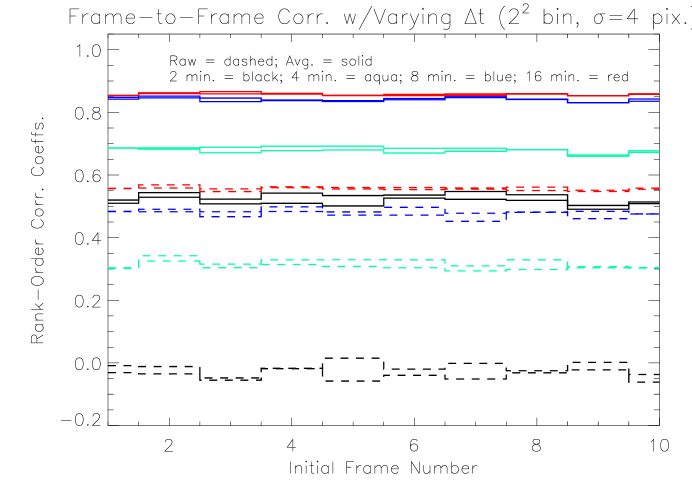
Figure 6: Plotted lines show frame-to-frame correlation coefficients for the $x$- and $y$- components of estimated flows, for varying time intervals $\Delta t$ between tracked magnetograms — 2 min in black, 4 min in aqua, 8 min in blue, 16 min in red. Dashed curves are from flows derived from un-averaged magnetograms, while solid curves are from flows derived from boxcar-averaged magnetograms. Flow estimates are more stable with averaged magnetograms and with longer $\Delta t$, until saturation occurs around $\Delta t$ = 8 min.

It would be convenient if an ideal choice of $\Delta t$ could be made a priori. As previously noted, however, flows with a range of speeds, and time and length scales are present at the solar photosphere (e.g., granular flows with speeds $\sim 1$ km sec^-1 with lifetimes of a few minutes and $\sim 1$ Mm length scales, and supergranular flows with speeds a few times $10^{2}$ m sec^-1 with lifetimes of about a day, and length scales of $\sim$ 10 Mm). Poor choice of $\Delta t$ can, however, be determined by post facto analysis of tracking results, meaning trial runs can be used to identify suitable timescales.

We first consider the noise-dominated regime, in which correlations between each velocity component from successive flow estimates will be small. Frame-to-frame correlations can be improved by increasing $\Delta t=t_{f}-t_{i}$, and by averaging successive magnetograms around $t_{i}$ and $t_{f}$ to synthesize initial and final images. Figure 6 shows frame-to-frame, rank-order correlations for the $x$- and $y$-components of estimated velocities, with $\sigma$ fixed at 4 pixels but for several $\Delta t$’s, using either unaveraged (dashed) and averaged (solid) magnetograms for $B(t_{i})$ and $B(t_{f})$. Low correlations for short values of $\Delta t$ imply that noise has degraded the velocity estimates. For $\Delta t=2$ min, the flow fields are even weakly anticorrelated. Increasing $\Delta t$ clearly increases frame-to-frame correlations, because real magnetic field evolution becomes more significant than spurious evolution from noise. Saturation occurs, however: doubling $\Delta t$ from 8 to 16 minutes did not greatly improve frame-to-frame correlations. As $\Delta t$ increases further, into the displacement-dominated regime, frame-to-frame correlations can approach unity, since displacements averaged over very long time intervals do not change much if the intervals’ endpoints are shifted slightly. To average the magnetograms, a 3-magnetogram boxcar was used for $\Delta t$ = 2 and 4 min, while a 5-magnetogram boxcar was used for $\Delta t$ = 8 and 16 min. For cadences of 2, 4, and 8 minutes, there is overlap in data used for $B(t_{i})$ and $B(t_{f})$. This probably leads to blurring of features from their motion over the summing interval, and could also lead to correlated noise in $B(t_{i})$ and $B(t_{f})$ (Schuck, 2006). The improvement in frame-to-frame correlations from averaging magnetograms is substantial. Linear correlation coefficients (not shown) were both lower and less consistent across frames. We therefore employ rank-order correlations to compute all subsequent autocorrelations. We provide concrete examples of these effects in Figures 7 and 8. In the former, successive flow fields computed with $\Delta t=2$ min show very little consistency between flow fields. In the latter, successive flows computed with $\Delta t=8$ min are much more consistent. Generally, frame-to-frame correlations are higher with larger values of $\sigma$ (not shown). This is consistent with FLCT detecting flows on larger spatial scales with larger $\sigma$, and larger-scale flows persisting longer in time. We discuss this issue in greater detail below.

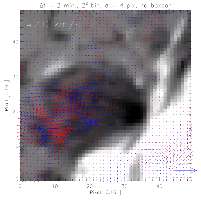
Figure 7: Successive flow maps in a subregion of the full field of view, derived from unaveraged magnetograms (binned $2\times 2$) separated in time by $\Delta t=2$ min with $\sigma=4$ pixels. Initial flows are shown by red vectors, subsequent flows are shown by blue vectors. Note significant variations between the flow fields in this noise-dominated regime.

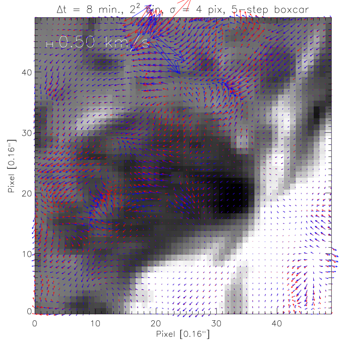
Figure 8: Successive flow maps from the same subregion, derived from averaged magnetograms (binned $2\times 2$) separated in time by $\Delta t=8$ min with $\sigma=4$ pixels. Initial flows are shown by red vectors, subsequent flows are shown by blue vectors. Note significant agreement between flow fields.

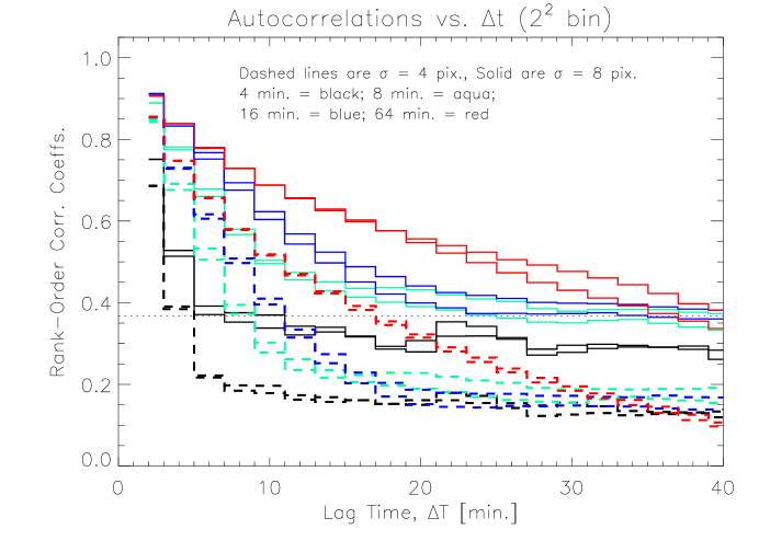
Figure 9: Plotted lines show correlation coefficients for the $x$- and $y$- components of flows estimated at $t_{i}$ and $t_{i}+\Delta T$, for several time intervals $\Delta t$ between tracked magnetograms — 4 min in black, 8 min in aqua, 16 min in blue, 64 min in red. Dashed curves are from flows derived with $\sigma=4$ pixels, while solid curves are from flows with $\sigma=8$ pixels. All flows were derived from boxcar-averaged magnetograms. Horizontal dotted line is $1/e$.

In the displacement-dominated regime, correlations between each velocity component from flow fields separated by lag times $\Delta T$ much shorter than $\Delta t$ can be high, but such correlations will be very weak when $\Delta T$ is on the order of $\Delta t$ or longer. This implies substantial flow evolution has occurred over the $\Delta t$ between magnetograms. Phrased another way, $\Delta t$ is longer than the estimated flows’ lifetimes. For estimated flows to reflect actual plasma velocities, however, $\Delta t$ cannot exceed the flow lifetime. Displacement-dominated flows are still physically meaningful, however: they quantify the average effects of flows over the course of more than one flow lifetime.

Having demonstrated the advantages of averaging, we use flows derived from magnetograms averaged with a five-step boxcar in our analyses of flow lifetimes below. For convenience, we will sometimes refer to flows inferred by FLCT as velocities, but the reader should keep in mind that FLCT’s flows should not necessarily be interpreted as estimates of plasma velocities at the center of the time interval $\Delta t$.

5.2 Estimating Flow Lifetimes

We define the lifetime $\tau$ of a flow as the lag time $\Delta T$ at which a one-parameter fit to the autocorrelation drops to $1/e\simeq 0.37$. In Figure 9, we plot autocorrelations for flow estimates made with two choices of $\sigma$ and several choices of $\Delta t$. For $\Delta t=64$ minutes, the lifetimes of the $x$- and $y$- flow components are around 35 minutes for $\sigma=8$, implying that flow estimates made with $\Delta t=64$ minutes are displacement-dominated. In contrast, the lifetimes of $\sigma=8$ flows estimated with $\Delta t=$ 4, 8, and 16 minutes are all at least as long as $\Delta t$. Lifetimes of flows estimated with $\sigma=4$ (dashed lines) are about half as long as $\sigma=8$ estimates for $\Delta t=$ 8, 16, and 64 minutes.

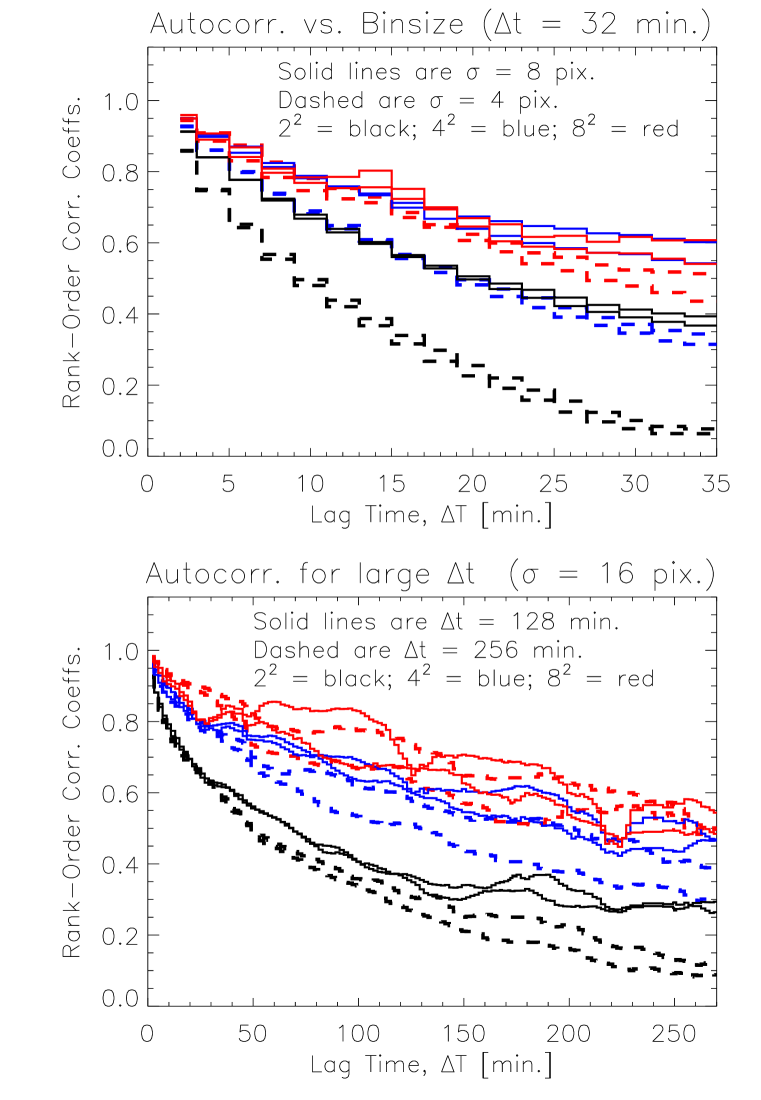
Figure 10: Top: Autocorrelations of $x$- and $y$-components of flows derived using two values of $\sigma$ (dashed = 4 pix., solid = 8 pix.) from magnetograms binned into different-sized macropixels (black = $2^{2}$, blue = $4^{2}$, red = $8^{2}$). Evidently, keeping $\sigma$ fixed but doubling bin size approximates keeping bin size fixed but doubling $\sigma$. Additional binning did not improve correlations. Bottom: Autocorrelations of $x$- and $y$-components of flows estimated with large values of $\sigma$ (16 pix. for all flows here) and from data rebinned into larger macropixel sizes (colors as in top panel) for $\Delta t=128$ min (solid) and $\Delta t=256$ min (dashed) are long-lived. As in top panel, additional binning did not improve correlations. All flows in both panels were derived from boxcar-averaged magnetograms.

The autocorrelations in Figure 9 also suggest that flows estimated on larger spatial scales — using a larger value of $\sigma$ — have longer lifetimes. In fact, this is typical. In addition, longer flow lifetimes are also found when data are rebinned into larger macropixels, though there is a point at which rebinning does not increase decorrelation times. The top panel of Figure 10 demonstrates that choosing larger values of $\sigma$ or rebinning into larger macropixels are practically equivalent. The bottom panel of Figure 10 implies that, when flows are displacement-dominated (i.e., they decorrelate at lag times $\Delta T<\Delta t$), longer-lived flows can be identified in rebinned data. We note that increasing the windowing parameter $\sigma$ can increase compute time for FLCT (and probably other tracking methods), while rebinning (holding $\sigma$ fixed) can decrease compute time, since fewer velocity estimates must be made.

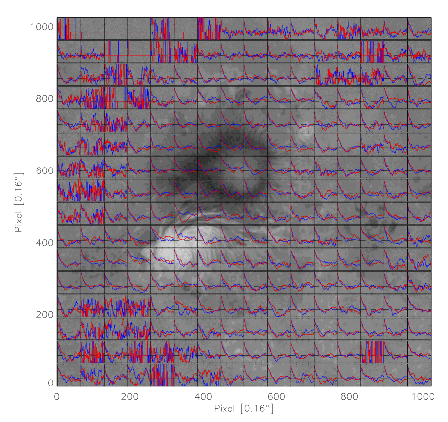
Figure 11: The grayscale image is $|B_{\rm LOS}|$ in a full-resolution magnetogram, with saturation at $\pm 4$ kG. Autocorrelations of $u_{x}$ (red) and $u_{y}$ (blue) in subregions of the full field of view. The flows were derived with $\Delta t=$ 64 min and $\sigma=4$ pix with $(2\times 2)$ binned data. The vertical range in each cell is [-0.5, 1.0], with a dashed black line at zero correlation. Autocorrelations are essentially random in weak-field regions, in which few pixels were above the threshold for tracking.

In Figure 11, we show autocorrelations of $u_{x}$ and $u_{y}$ in $(32\times 32)$-pixel subregions of magnetograms with 0.32 ″pixels (so binned $2\times 2)$. These flows were derived with $\Delta t=$ 64 minutes and $\sigma=4$ pixels. Background gray contours in the figure show 50 G and 200 G levels of $|B_{\rm LOS}|$ from the initial magnetogram (in full-resolution pixels), so variations in flow autocorrelations can be understood in the context of active region structure.

In weak-field regions, few pixels are above the threshold for tracking, so very few velocities are estimated. Consequently, the autocorrelations are essentially random. We therefore only fitted the autocorrelations in high-occupancy subregions, which we define to be those with a median (over the dataset’s duration) occupancy of pixels above the tracking threshold of at least 20%, which gives large enough samples that the autocorrelations are stable. The fits to the magnetic field autocorrelation curves in Figure 4 convey how well the single-parameter exponential fits match the autocorrelations for a range of lifetimes and autocorrelation profiles.

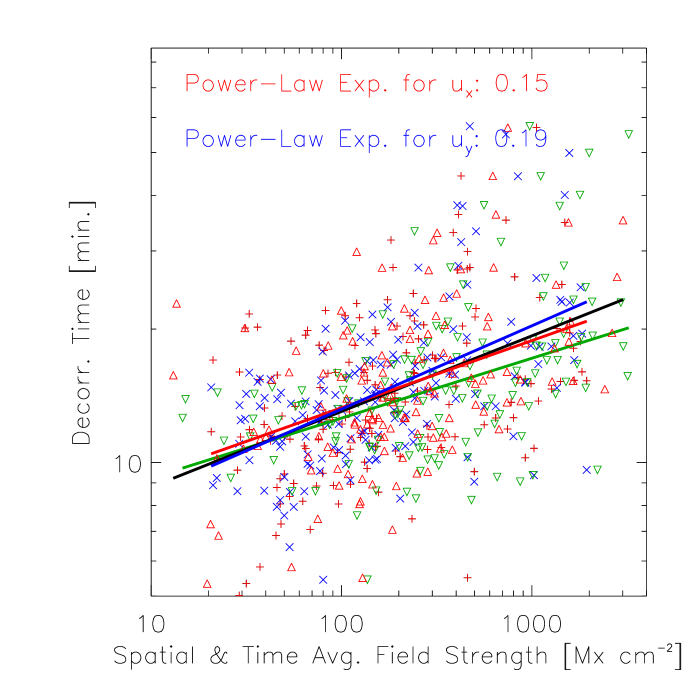
Figure 12: Fitted flow lifetimes for non-bubble subregions of Figure 11 in which at least 20% of the $32^{2}$ $(2\times 2)$ pixels exceeded the tracking threshold, as a function of the spatial average of the unsigned, boxcar-averaged LOS magnetic field in each subregion. Lifetimes for $u_{x}$ in subregions are shown with red +’s, $u_{y}$ are blue $\times$’s, and fits to these are red and blue solid lines. The red $\Delta$’s (green $\nabla$’s) are lifetimes of $u_{x}$ versus subregion-averaged $|B_{z}|$ ($|{\mathbf{B}}|$) from the SP data, and the black (green) line is a fit, with slope 0.17 (0.13). The correlation between flow lifetime and field strength is statistically significant, though the fitted power-law dependence is weak.

In Figure 12, we show fitted flow lifetimes ($u_{x}=$ red +’s and $u_{y}=$ blue $\times$’s) for high-occupancy subregions of Figure 11, as a function of the spatial average of the unsigned, boxcar-averaged LOS magnetic flux density in each subregion. Red $\Delta$’s and green $\nabla$’s are lifetimes of $u_{x}$ components of the flow as functions of spatial averages of $|B_{z}|$ and $|{\mathbf{B}}|$, respectively, and red dashed and green solid lines are fits to each. Most flow lifetimes are between about 7 and 30 minutes, confirming the expectation based upon the red, dashed curves in Figure 9 that these flows are displacement-dominated. There are statistically significant correlations both between flow lifetime and field strength, and between flow lifetime and median occupancy of above-threshold pixels. The rank-order correlation of field strength $|{\mathbf{B}}|$ with $u_{x}$ (and $u_{y}$) flow lifetime, however, is a statistically significant 0.52 (and 0.51) for the 35 of 137 non-bubble subregions of SP data with occupancies of 1000 or more (of a possible 1024), implying the lifetime versus field-strength trend is independent of any occupancy-lifetime correlation. Linear fits to logarithms of lifetime as a function of field strengths return weak power-law exponents, below $\sim 0.2$ for each flow component. For flows with $\Delta t=$ 8 minutes and $\sigma=$4 pixels, correlations of lifetime with field strength are quite weak. For flows estimated with $\Delta t=$ 256 minutes and $\sigma=$16 pixels, fitted power-law exponents between lifetime and field strengths $\{|B_{\rm LOS}|,|B_{z}|,|{\mathbf{B}}|\}$ range from $0.2--0.3$, but field strength-lifetime correlations are weaker for $u_{x}$ than for $u_{y}$. The east-west orientation of the PIL, combined with apparent rapid motion of vertical magnetic flux along the PIL (Démoulin and Berger, 2003), could produce more rapid evolution of east-west flow components than north-south flow components.

Correlations between flow lifetime in a subregion and magnetic field strength in that subregion imply that Lorentz forces drive a component of photospheric evolution. To the extent that convection is the primary driver of photospheric evolution, and magnetic fields inhibit convection, there is no obvious reason why flow lifetimes should be longer in stronger-field regions. But because magnetic structures persist for longer timescales than flows, it is likely that forces acting on those fields, such as magnetic buoyancy (Parker, 1955) or magnetic torques (Longcope and Welsch, 2000) are also longer-lived. Consequently, it is physically reasonable that in stronger-field regions, magnetic evolution is partially driven by longer-acting forces than the pressure gradients arising from convection.

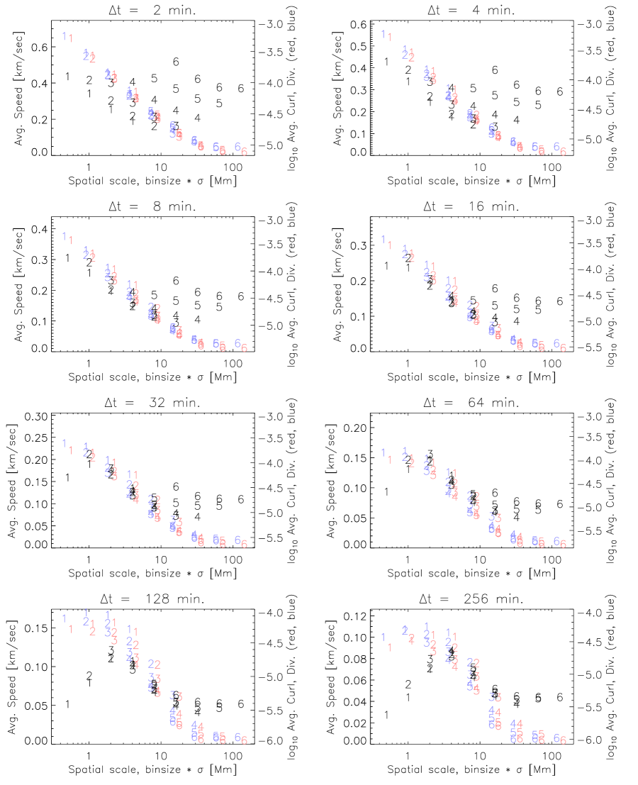
Figure 13: Black numerals show average flow speed (left axis) vs. spatial scale, parametrized by the product of the macropixel bin size and the windowing parameter $\sigma$, for several flow cadences; the numbers correspond to $\log_{2}$(bin size), in units of 0.16 ″pixels. Red (blue) numerals show the log of the average normal curl (horizontal divergence) of the flow, on the right scale, and are slightly offset right (left) for clarity. Because we estimated flows for several macropixel sizes and $\sigma$’s, we have multiple samples at most resolutions. For shorter $\Delta t$, bin size affects the average flow speed at a fixed spatial scale; for longer $\Delta t$, bin size does not strongly affect average flow speed at a fixed spatial scale. In contrast, binning seems to affect average flow curls and divergences more at larger $\Delta t$.

How does flow lifetime $\tau$ depend upon flow spatial scale? A crude estimate of the turnover time of a convective eddy — expected to be related to flow lifetime — is the eddy length scale $L$, divided by a characteristic speed $u_{0}$. As noted by Berger et al. (1998), however, “the term ‘characteristic speed’ must be used only in relation to a given spatiotemporal resolution.” So as a preliminary step in characterizing flow lifetime versus spatial scale, we first investigate flow speed versus spatial scale. What do our results reveal about typical flow speeds over varying spatial scales? We define a flow’s spatial scale as the product of macropixel bin size and the windowing parameter $\sigma$. As shown in Figure 10, changes in both parameters seem to have similar effects upon flow lifetimes. Because we estimated flows for several macropixel sizes and choices of $\sigma$, we therefore have multiple sequences of flow estimates at a few spatial resolutions for each cadence $\Delta t$. We computed the average flow speed at each scale over all pixels and time steps for which velocities were estimated. In Figure 13, we show average velocity as a function of spatial scale; the plot symbols are $\log_{2}$(bin size), in units of the data’s native 0.16 ″pixels, to better illustrate changes in average velocity as a function of bin size at a given spatial scale. (Values of curls and divergences of the flow pattern are also shown in this figure, and are discussed below.) One basic property is evident: average speeds are slower for longer tracking intervals $\Delta t$, as was noted by Chae et al. (2004) and Verma and Denker (2011) for both relatively long and short $\Delta t$, respectively. (This is discussed further below.) For $\Delta t$ shorter than 16 min, average speeds peak at the small end of the range of spatial scales, as found in previous work (Berger et al., 1998; Chae et al., 2004; Verma and Denker, 2011). For longer $\Delta t$, however, average speeds peak at higher spatial scales: speeds at small-scales for large $\Delta t$ are low. The large $\Delta t$ implies that small-scale structures at $t_{i}$ and $t_{f}$ have evolved substantially. While it is plausible that FLCT would infer random displacements in this case, and that averaging over these random displacements (all positive) would produce a large mean speed, we do not observe this. Apparently, for a given $\Delta t$, the FLCT code is primarily sensitive to flows on a particular spatial scale. Also, for shorter $\Delta t$, average speed at a given spatial resolution depends strongly upon spatial binning, while for longer $\Delta t$, average speeds seem insensitive to spatial binning. This probably reflects different effects from the combination of actual evolution and noise on the apparent magnetic evolution convolved with spatial binning and apodization by $\sigma$. For instance, large values of $\sigma$ presumably average over the effects of actual evolution on sub-$\sigma$ scales. If so, speeds should be higher with smaller $\sigma$ at a given spatial resolution, as we find. We remark that the combined effects of cadence with binning and apodization preclude straightforward testing our FLCT velocities for consistency with the Kolmogorov scaling (e.g., Thompson 2006, p.68).

We note that tests of FLCT with synthetic magnetograms from MHD simulations, in which the true velocities were known, showed that FLCT systematically underestimates speeds, by $\sim 25$% (Welsch et al., 2007), so the absolute values of the average speeds we find here are probably systematically lower than estimates that would be found using other tracking codes. Further, because our velocities are derived from magnetic evolution, and magnetic flux both tends to inhibit convection and to concentrate in stable downflow regions between convective cells, it is reasonable to expect our average speeds to be systematically lower than tracking results derived from intensity images. We note that for $\Delta t$ of 2 or 4 min, our average speeds at the smallest spatial scale are close to those reported by Verma and Denker (2011) (see their Table 3). The speeds of FLCT flows derived by Welsch et al. (2009), with $\Delta t$ of 96 min and a spatial scale of $\sim$12 Mm were predominantly in the 50 – 100 m sec^-1 range (see their Fig. 6), comparable to values we find for similar $\Delta t$ and spatial scales here.

In Figure 14, we show the average speed versus tracking cadence $\Delta t$, averaged over both space and time in all flow maps at a given spatial resolution and all spatial resolutions at each cadence. Effectively, this amounts to computing the average of speeds at each $\Delta t$ in Figure 13 — fitting the speeds in each panel to a horizontal line. Error bars in Figure 14 reflect the standard deviation in speeds in each panel of Figure 13. A linear fit to the logarithms of cadences and average speeds returns an power-law exponent of -0.34. Verma and Denker (2011) computed average speeds for a range of much shorter $\Delta t$’s, and over the eight-fold increase in $\Delta t$ from 60 to 480 sec, their average speed fell by about a factor of two. This implies a scaling near -1/3, similar to ours. (But they found an increase in average speed between $\Delta t$’s of 15 and 60 sec, and similar average speeds at 60 and 90 sec.) They suggest decreasing speeds with increasing $\Delta t$ might arise from the short lifetimes of features in the images they track. However, we find the same effect when tracking much longer-lived magnetogram structures, implying the limited lifetimes of features is probably not solely responsible for decreasing speeds with increasing $\Delta t$. We also note that both Hagenaar and Shine (2005) and Verma et al. (2011) found that individual, successive moving magnetic features (MMFs) followed preferential paths as they moved outward from sunspots, suggesting short-lived features can reveal longer-lived flow patterns. As noted above, a longer $\Delta t$ can average over the effects of short-lived flows: displacements inferred with a longer $\Delta t$ might not recover zig-zag motions that can be resolved with shorter $\Delta t$, with the shorter apparent path length at longer $\Delta t$ implying a lower estimate of speed.

Verma and Denker (2011) also averaged higher-cadence flow maps over increasing time periods — 1, 2, 4, 8, and 16 hr — and found statistics of averaged-flow speeds (mean, median, 10th percentile, maximum) all systematically decreased. Such averaging is not the same as tracking over longer $\Delta t$, as we have done, but the trends are qualitatively similar: a log-log plot of the averaging periods and mean speed from tracking granulation given in Table 1 of Verma and Denker (2011) also shows a power-law decrease of mean speed with time between 1 – 8 hr, though a linear fit to the logarithms returns an exponent near -0.18, about half our result. It is plausible that short-lived flows, resolved with shorter $\Delta t$, would primarily reflect the essentially random effects of granulation, and therefore average incoherently over long times. However, comparison of our large-$\Delta t$ flow speeds with speeds inferred by Verma and Denker (2011) with a shorter tracking interval $\Delta t^{\prime}$ and then averaged over longer time intervals similar to ours implies that shorter-timescale flows are averaging coherently. It is possible that the motion tracers — either the intensity pattern, or magnetic flux — used in one approach or the other (or even both!) do not faithfully represent the true plasma velocity. In this vein, Rieutord et al. (2001) has argued that the motion of granules does not accurately reflect underlying velocities on spatial and temporal scales that are too short. This suggests flows inferred from magnetic tracking by flow maps derived with short tracking intervals but averaged over long $\Delta t$ and flow maps derived with a tracking interval of $\Delta t$ should be compared in a future study.

Figure 14: Flow speed as a function of cadence, averaged over both space and time for each spatial resolution (binning $\times\sigma$) and over spatial resolutions at each $\Delta t$. Error bars show standard deviation over resolutions. Least squares linear fit to the logarithms of cadence and speeds returns a power-law exponent of -0.34.

Figure 15: Flow lifetimes (+’s for $u_{x}$, $\times$’s for $u_{y}$) as a function of flow spatial scale, as parametrized by the product of the macropixel bin size and the windowing parameter $\sigma$, for several flow cadences. Because we estimated flows for several macropixel sizes and $\sigma$’s, we have multiple samples at some resolutions. We computed linear fits (solid lines) to the logarithms of spatial scale and lifetime over a limited range of scales. The fitted power-law exponent is printed in the title of each cadence’s plot.

We now return to the question of how flow lifetime $\tau$ varies with spatial scale. As above, we define the spatial scale of an estimated flow as the product of macropixel size and windowing parameter $\sigma$, and therefore have multiple sequences of flow estimates at a few spatial resolutions for each cadence $\Delta t$. For each sequence of flow estimates, we can estimate the flow lifetime $\tau$ over the whole active region from a one-parameter fit to the autocorrelation as function of lag time $\Delta T$, assuming exponential decay, $\exp{(-\Delta T/\tau)}$. In Figure 15, we plot flow lifetimes estimated this way, as a function of spatial scale, for several tracking cadences $\Delta t$. In the shorter-scale region of each log-log plot, flow lifetime seems to scale, roughly, in a straight line with spatial scale. To characterize this dependence, we fit power-law exponents for each cadence over the range of seemingly straight-line log-log scaling (shown with a solid line on each plot). For longer cadences, flow lifetime appears to scale nearly linearly with scale length, while the dependence of flow lifetime on length scale seems weaker for shorter cadences. At larger length scales in each plot, the relationship between lifetime and length scale becomes less coherent as binning and apodization are varied. Welsch et al. (2009) found lifetimes at $\sim$ 12 Mm to be two to three steps at their $\Delta t$ = 96 min magnetogram cadence. For similar spatial scale and $\Delta t$ (64 and 128 min) we find shorter lifetimes, by a factor of two or so, although this is also the spatial scale where our lifetime estimates become incoherent. For all spatial scales we investigate, the flow lifetime is shorter than that predicted from a linear scaling of lifetime with length scale, sometimes dramatically so. We note that our estimates of lifetimes are rough approximations. Longer-lived flows (e.g., supergranular flows) would remain undetected in our lifetime estimates if their asymptotic autocorrelation lies below our $1/e$ cutoff. The longer lifetimes of larger-scale flows is another possible explanation of the correlation between flow lifetime and magnetic field strengths: stronger magnetic fields might couple nearby regions of plasma more strongly (making the plasma more rigid), leading to larger spatial scales for flows in more strongly magnetized regions; and such flows should persist for longer than smaller-scale flows.

In Figure 16, we show fitted flow lifetimes for $x$ and $y$ components of the flow (denoted $+$ and $\times$, respectively) as functions of $\langle v\rangle$, the flow speed averaged over space and time for each combination of tracking interval $\Delta t$, spatial binning, and apodization parameter $\sigma$. Plot symbols are color-coded by spatial scale, defined as the product of spatial binning and apodization parameter. Generally, higher average speeds correspond to shorter lifetimes. While a range of lifetimes was found at each average speed, there appears to be a rough upper limit at a given speed, with the peak fitted lifetime $\tau_{*}$ scaling roughly as $\langle v\rangle^{-2}$. Noting that the product of a timescale and the square of speed yields a quantity with the dimensions of kinematic viscosity (length²/time), the mean and standard deviation of $\tau_{*}\langle v\rangle^{2}$ are $(2.7\pm 1.9)\times 10^{11}$ cm² sec^-1 and $(2.9\pm 2.3)\times 10^{11}$ cm² sec^-1 for the $x$ and $y$ components of the flow, respectively. The limit of flow lifetimes shown by the dashed line in Figure 16, $1.25\langle v\rangle^{-2}$, would correspond to a kinematic viscosity of $7.5\times 10^{11}$ cm² sec^-1. While the physical significance of this value is unclear (if it is even physical — it might be an artifact of our methods), it roughly agrees with values of viscosity near the photosphere reported by Nesis et al. (1990).

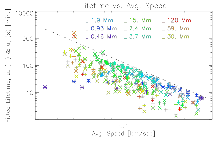
Figure 16: Fitted lifetime vs. flow speed averaged over space and time for each choice of $\Delta t$, spatial binning, and $\sigma$. Lifetimes for $u_{x}$ and $u_{y}$ are plotted with $+$’s and $\times$’s, respectively. Generally, higher average speeds correspond to shorter lifetimes. While a range of lifetimes exists at each average speed, there appears to be an upper limit at a given average speed, with the peak fitted lifetime scaling roughly as (average speed)^-2 (dashed line; note that this line is not a fit). Points are color-coded by spatial scale of the flow (binning $\times\sigma$).

5.3 Lifetimes of Curls & Divergences

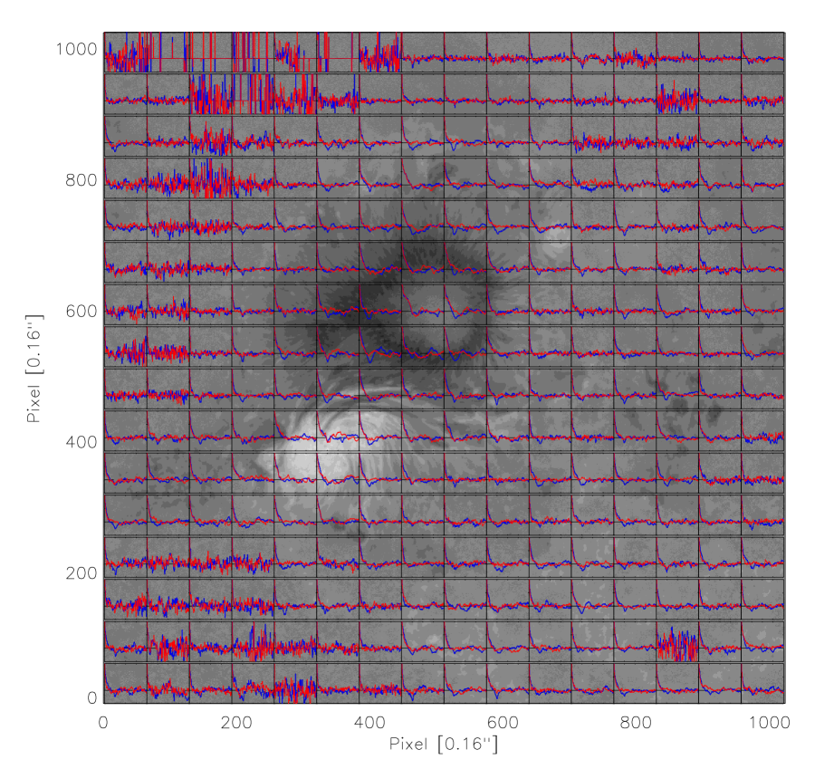
Figure 17: The grayscale image is $|B_{\rm LOS}|$ in a full-resolution magnetogram, with saturation at $\pm 4$ kG. Autocorrelations of normal curls (red) and horizontal divergences (blue) in each subregion of the full field of view are overplotted. The flows were derived with $\Delta t=$ 64 min and $\sigma=4$ pix. The vertical range in each cell is [-0.5, 1.0], with a dashed black line at zero correlation. Autocorrelations are essentially random in weak-field regions, in which few pixels were above the threshold for tracking.

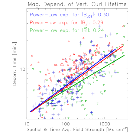
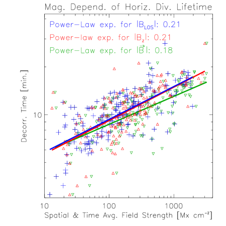
Figure 18: Fitted lifetimes of normal curls (left) and horizontal divergences (right) for subregions of Figure 17 in which at least 20% of the $32^{2}$ $(2\times 2)$ pixels exceeded the tracking threshold, as functions of the spatial average $|B_{\rm LOS}|$ (from NFI; blue +’s), $|B_{z}|$ (from SP; red $\Delta$’s), or $|{\mathbf{B}}|$ (from SP; green $\nabla$’s) in each subregion. The correlation between curl/divergence lifetime and field strength is statistically significant, though the fitted power-law dependence is weak. The magnetic dependence of the lifetimes of curls is somewhat stronger than that of lifetimes of divergences.

The lifetimes of normal curls and horizontal divergences of the flow fields, defined as

$$\,\hat{\mathbf{n}}\cdot(\nabla_{h}\times{\mathbf{u}})$$ (4)

$$(\nabla_{h}\cdot{\mathbf{u}})~{},$$ (5)

respectively, are also of interest: vortical flows can efficiently inject magnetic energy and helicity (e.g., Longcope and Welsch 2000), and diverging flows are associated with flux emergence in both simulations (Abbett et al., 2000) and observations (Welsch et al., 2009). In Figure 13, we have overplotted mean absolute values of curls (divergences), averaged over tracked pixels in $x-y-t$ datacubes of our flow maps, in red (blue), computed using finite difference approximations with the smallest binning, twice the native 0.16 ″pixel size, in the denominator. For consistency with our definition of spatial scale used above, the denominator should be the product of macropixel size and apodization parameter $\sigma$. This would, however, introduce an additional inverse scaling with the variable plotted on the horizontal axis. Average values of curls and divergences at our smallest length scales for short $\Delta t$ are on the order of a few times 10^-4 sec^-1, similar to values reported by Verma and Denker (2011). For fixed $\Delta t$, curls and divergences fall by roughly two decades over the approximately two decades in length scales we study, implying curl and divergence magnitudes scale approximately as 1/length. Average magnitudes of curls and divergences decreased by about a decade over the range of $\Delta t$’s in our study, a faster decrease with $\Delta t$ than for speeds.

In Figure 17, we show autocorrelations of normal curls (red) and horizontal divergences (blue) computed in subregions of the full FOV, superimposed on 50 G and 200 G contours of $|B_{\rm LOS}|$, for flows estimated from 2²-binned data, with $\sigma=4$ macropixels and $\Delta t$ = 64 min. In Figure 18, we show the fitted lifetimes for curls (left) and divergences (right) versus subregion- and boxcar-averaged $|B_{\rm LOS}|$ from NFI, and subregion-averaged $|B_{z}|$ and $|{\mathbf{B}}|$ from SP, where, as above, lifetimes were determined by one-parameter fits to subregions’ autocorrelation functions assuming exponential decay. As with the lifetimes of $x$ and $y$ components of the flow, curl and divergence lifetimes exhibit a dependence on both field strength and the median occupancy of above-threshold pixels in each 32² subregion of $2\times 2$-binned full-resolution pixels. The rank-order correlation of field strength $|{\mathbf{B}}|$ with curl (divergence) lifetime, however, is a statistically significant 0.59 (0.58) for the 59 subregions with occupancies of 1000 or more (of a possible 1024), implying the lifetime versus field-strength trend is independent of any occupancy-lifetime correlation. We repeat that our estimates of $|B_{\rm LOS}|$ suffer from non-monotonicity in the Stokes $V/I$ ratio, while our spatial averages of $|B_{z}|$ and $|{\mathbf{B}}|$ ignore the likelihood of small filling factors for magnetic field structures. Despite these limitations, the existence of a trend seems clear, and we find a stronger dependence of the lifetimes of curls on field strength than for lifetimes of divergences. We note that, as with the lifetime of flows themselves, the fitted dependence of lifetime of curls and divergences on $|{\mathbf{B}}|$ appears weaker than that on either $|B_{z}|$ or $|B_{\rm LOS}|$.

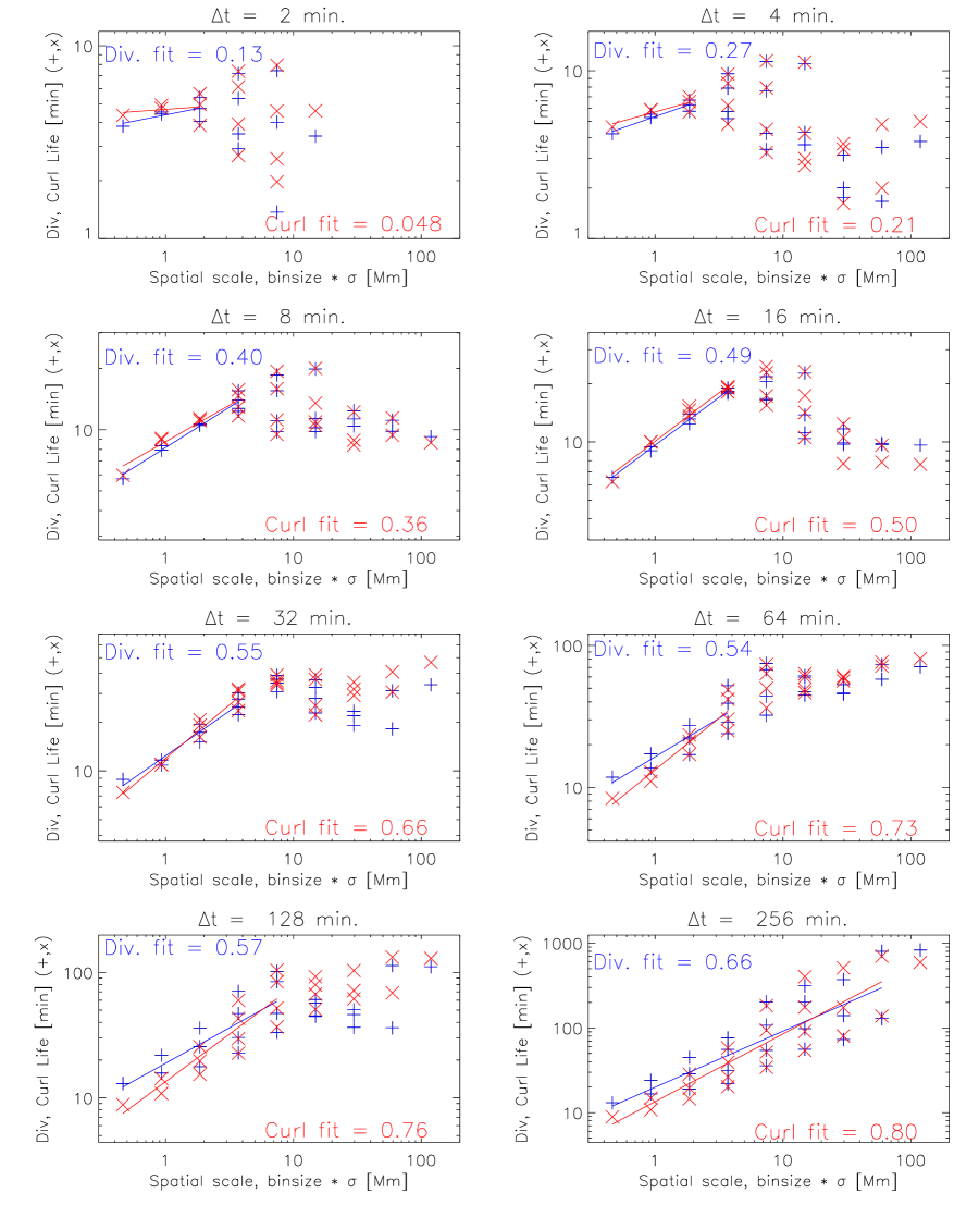
Figure 19: Lifetimes of normal curls (red $\times$’s) and horizontal divergences (blue +’s) as a function of flow spatial scale, as parametrized by the product of the macropixel bin size and the windowing parameter $\sigma$, for several flow cadences. Because we estimated flows for several macropixel sizes and $\sigma$’s, we have multiple samples at some resolutions. We computed linear fits (solid lines) to the logarithms of spatial scale and lifetime over a limited range of scales, and list the fitted power-law exponents on each cadence’s plot.

Finally, in Figure 19, we show the lifetimes of normal curls (red $\times$’s) and horizontal divergences (blue +’s) versus spatial scale, defined as above as the product of macropixel bin size and windowing parameter $\sigma$, for each tracking interval $\Delta t$. Because we estimated flows for several macropixel sizes and $\sigma$’s, we have multiple samples at some resolutions, most of which roughly agree. At most cadences, the lifetimes increase with spatial scale, and then saturate. In Figure 19, we also show linear fits to the logarithms of lifetimes as functions of logarithms of spatial scales over the range of spatial scales before saturation occurs.

6 Summary & Discussion

We used FLCT to estimate flows from a $\simeq 13$ hour sequence of high-cadence ($\simeq 2$ min), high-resolution (0.16 ″pixel, 0.3 ″diffraction limit) line-of-sight magnetograms of NOAA AR 10930. This seeing-free, high-resolution, long-duration dataset enabled us to conduct a detailed study of the effects of tracking parameter selection on the estimated flows, and to investigate the lifetimes of flows and flow structure (normal curls and horizontal divergences) as functions of spatial scale and magnetic field strength. For context, we also characterized the lifetimes of magnetic structures.

Several conclusions can be drawn from our results, which may be divided into practical conclusions relevant to the process of flow estimation from magnetograms, versus physical conclusions about surface magnetic flows and evolution. Our practical conclusions are:

• Flows estimated by magnetic tracking (and related optical flow) methods with a particular set of tracking parameters (i.e., tracking interval $\Delta t$ between images, pixel size, apodization window size $\sigma$) are primarily sensitive to evolution on a particular spatial scale and time scale.

• If the tracking interval $\Delta t$ between pairs of magnetograms is too short, then changes in the field between magnetograms is mostly due to noise instead of actual magnetic evolution. This is the noise-dominated regime. Its hallmark is rapid fluctuations in estimated velocities, which can be quantified by autocorrelating maps of the velocity components. The effect of noise can be reduced by: increasing $\Delta t$, averaging successive magnetograms prior to tracking, or both.

• Because magnetic features persist for much longer than the intensity features to which tracking methods have also been applied (e.g., Berger et al. 1998; Verma and Denker 2011), the upper limit for $\Delta t$ is not strongly constrained in magnetic tracking. If, however, the tracking interval $\Delta t$ between pairs of magnetograms is longer than the flow lifetime at that spatial scale, then the estimated flows reflect an average velocity over more than one flow lifetime. This is the displacement-dominated regime. Although this time-averaged velocity is physically meaningful, it does not represent the actual plasma velocity field at a particular time (e.g., the center of the tracking interval).

• Hence, choice of $\Delta t$ can determine whether flow estimates are noise-dominated ($\Delta t$ too short), displacement-dominated ($\Delta t$ longer than the flow lifetime), or representative of actual flows. To estimate actual plasma velocities, appropriate choice of $\Delta t$ can be established through post-facto analysis of flow maps, by autocorrelating flows to find a $\Delta t$ that both maximizes frame-to-frame autocorrelations (which thus minimizes the effects of noise) and is less than the flow lifetime $\tau$, which we take to be the time at which the autocorrelation drops to $1/e$.

• Average estimated speeds decrease with increasing tracking interval $\Delta t$ between magnetograms (see Figure 14).

Our physical conclusions are:

• As noted by previous researchers (e.g., Berger et al. 1998), photospheric flows operate over a range of spatial scales, and exist for a range of lifetimes. Hence, referring to “the flow field,” by itself, is imprecise: explicit reference to spatial and temporal scales must also be made.

• Magnetic structure persists substantially longer in stronger-field regions generally, and longer in regions of strong vertical field $|B_{z}|$ than in regions of strong magnetic field strength $|{\mathbf{B}}|$.

• Magnetic structure persists substantially longer when averaged over larger spatial scales. Flow components and their derivatives estimated on larger spatial scales also persist for significantly longer, though lifetimes scale less than linearly with length scale.

• Flow components, horizontal divergences, and normal curls persist somewhat longer in regions with stronger fields: our estimates of their lifetimes are significantly statistically correlated with spatially averaged values of each of $|B_{\rm LOS}|$, $|B_{z}|$, and $|{\mathbf{B}}|$. We find the lifetimes of curls exhibit a slightly stronger dependence on field strength than either flows components or horizontal divergences.

• Flows with faster average speeds typically exhibit shorter lifetimes. Also, there appears to be a rough upper limit on flow lifetime at a given average speed, which scales as the inverse of the square of the average speed.

In this study, we found sets of differing velocity fields for a single magnetogram dataset by applying a single correlation tracking method over various spatial and temporal scales. This is not surprising: coherent flow structures on varying scales are known to be present in the photospheric flow field, e.g., global-scale Sun’s differential rotation (in our synodic frame) and meridional flow, high-speed granular flows and lower-speed supergranular flows driven by convection, and possibly flows arising from Lorentz forces in magnetized regions. In addition, turbulent flows are likely present. This, however, raises the question, “Given that a family of velocity fields can be derived on several scales, how can one determine the best estimate of the velocity field?” But what determines “best?” It is tempting to try to estimate the “true” velocity field in each resolution element (pixel), but what does this mean physically? Assuming the photospheric plasma behaves exactly as a fluid down to some kinetic scale, then within our smallest resolution element there is a distribution of subresolution velocities, and a meaningful definition of the “true” velocity must be defined in terms of this distribution. If the distribution of velocities is peaked in speed and direction, then some statistical property of each (e.g., mean or median) might meaningfully quantify the flow. It is, however, probable that sub-resolution flows are consistent with a power-law distribution of flow energy with spatial wavenumber, similar to that proposed by Kolmogorov (though perhaps with a different wavenumber scaling), through some inertial range down to a dissipation scale. A reasonable expectation based upon our results, as well as those of previous studies (Berger et al., 1998; Verma and Denker, 2011), is that flows on successively smaller scales will have higher speeds. In this case, what we infer from the motion of magnetic flux (or of brightness variations, if tracking intensity) is an “effective flow” — the combined effect of flows acting on all scales. But it is probable that the effective flow does not correspond to “the” physical velocity.

From the practical standpoint of understanding how flows are related to other phenomena of interest (e.g., flares, CMEs, coronal heating, the dispersal of active region magnetic flux), we must investigate relationships between these phenomena and flows on varying spatial and temporal scales to understand which (if any) scales are most relevant. A key challenge is that the largest velocities are present at the smallest scales: while in a sense these strongest flows are the easiest to detect, they also have the shortest lifetimes, and are therefore probably the least relevant for some processes with longer characteristic time scales, e.g., the emergence of large-length-scale magnetic flux systems in active regions. Computing the Poynting flux, for instance, based upon an instantaneous estimate of flows on granular scales will likely give an incomplete (if not misleading) picture of how much and where magnetic energy is being transported across the photospheric layer. Hence, much work remains to understand photospheric flows and their relationships to processes like the transport of magnetic energy across the photosphere.

We remark that the techniques we have applied here can also be applied to both real and simulated vector magnetogram sequences, to better understand evolution of both magnetic fields and flows. Long sequences of vector magnetograms (from, e.g., HMI) could be tracked to analyze flow properties over a range of spatial and temporal scales as functions of the vector magnetic field’s properties. The lifetimes of magnetic and flow fields from simulations of photospheric evolution (e.g., Cheung et al. 2010) can also by analyzed via autocorrelation for comparison with lifetimes inferred from observations.

We expect observations using the newest generation of ground-based solar telescopes — NST Goode et al. (2010), GREGOR (Volkmer et al., 2010), ATST (Rimmele et al., 2010), and EST (Zuccarello and Zuccarello, 2011) — to play a key role in future studies of flows at high resolution.

Appendix A Calibration by Co-alignment with SP Vector Magnetograms

Schrijver et al. (2008) used SP data to produce vector magnetograms of AR 10930 over 12 – 13 Dec. 2006, which are available online. One of the magnetograms they produced overlaps with our tracking run. Here, we describe the procedure we used to interpolate magnetic field data from that magnetogram onto a downsampled, cropped grid corresponding to our NFI observations. Note that our ultimate goal is to be able to relate the lifetimes of magnetic field structures and flows over regions of the NFI FOV to average magnetic properties in those regions. Hence, we do not seek pixel-scale agreement between the SP and NFI magnetograms. Rather, we seek approximate agreement on the scales of a few arcseconds.

Schrijver et al. (2008) report sampling the SP data into 0.63 ″pixels. We resampled NFI observations of $B_{\rm LOS}$ at the start, middle, and end of the 45-minute SP scanning interval from the original 0.16 ″pixels into $(4\times 4)$ bins to achieve commensurate resolution. Comparison of features in the $B_{z}$ map from SP (Figure 20, upper left) with binned $B_{\rm LOS}$ maps from NFI at the start and end of the scan (Figure 20, middle and bottom of left column) shows that most of the discrepancies between the SP and NFI data are in the horizontal direction: features in the SP image extend over $N_{x,SP}=295$ pixels in the horizontal direction, while the NFI images of the corresponding features are only $N_{x,NFI}=240$ pixels in horizontal extent.

Given the position of the AR near 20^∘ W from disk center at the time of the scan, and the $\sim 10^{\circ}$ extent of the AR, the cumulative effect of horizontal distortion in pixel lengths from foreshortening in NFI pixels compared to reprojected SP pixels over the FOV should account for a $\sim 9$% difference, or about 22 pixels. Hence, additional distortion is present. We also note that, even if reprojection fully accounted for the SP/NFI discrepancies, un-reprojecting the SP data would require a difficult inversion of the convolved effects of solar rotation, spacecraft pointing, and spectrograph rastering over the 45 minute scanning period.

We therefore adopt an ad hoc approach, using repeated Fourier interpolations to spatially interpolate the SP data onto each column of the NFI grid. We first interpolated the SP data onto $N_{x,NFI}$ evenly-spaced shifts $N_{x,SP}/N_{x,NFI}$ apart (one Fourier interpolation per shift), but found systematic residual horizontal distortions were present, consistent with a higher-order variation in distortion across the image. We therefore included a quadratic term in the spacing between interpolations: where $x_{i}$ is the location of the $i$-th column of NFI data, we interpolated the SP data at $x_{i}^{\prime}=N_{x,SP}/N_{x,NFI}(ax_{i}+bx_{i}^{2})$. By trial and error, we found $a=0.925$ and $b=0.06$ gave good qualitative agreement between $\pm$100 G and $\pm$400 G contours of $B_{\rm LOS}$ from NFI at the middle of the scan interval with $B_{z}$ from the SP magnetogram, as shown in the upper right panel of Figure 20. It may be seen that the NFI’s contours of $B_{\rm LOS}$ do not match SP’s $B_{z}$ everywhere, but the remaining offsets do not appear to be systematic across the image, or along columns. (We note that the non-monotonicity in the NFI signal precludes use of some quantitative measures of NFI-SP agreement [e.g., cross-correlation, or minimized square difference] since optimal alignment probably corresponds to the weakest umbral field in NFI being co-aligned with the strongest umbral field in SP, while features outside of the umbra should generally correspond one-to-one.)

As discussed above, we are primarily interested in average magnetic properties (vertical field strength, total field strength) in larger-scale regions of the NFI FOV, so we only use the interpolated SP data binned into $(8\times 8)$ and $(16\times 16)$ macropixels. Comparisons of $(32\times 32)$-binned NFI $|B_{\rm LOS}|$ data with $(8\times 8)$-binned $|B_{z}|$ (and $|{\mathbf{B}}|$) from SP in the middle-right (and bottom-right) panel of Figure 20 shows good spatial agreement at that resolution.

Note that the SP data do not fully cover the NFI FOV, which is 256² pixels when binned $(4\times 4)$. Consequently, we can only use the SP data on a subset of the full NFI FOV.

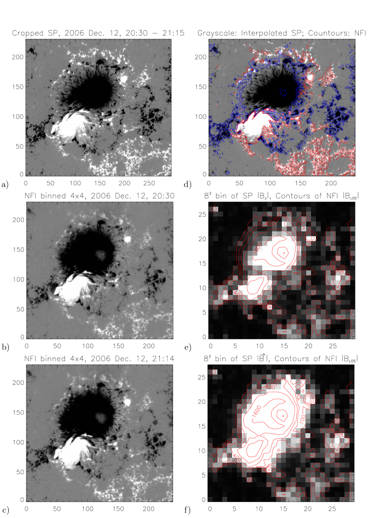
Figure 20: Left column: a) SP map of $B_{z}$, scanned over 45 minutes. b) & c) NFI images binned to $(4\times 4)$ from 0.16 ″pixels, from the beginning and end of the SP scan. Note lateral extent of SP data is 295 pixels, while NFI data are 240 pixels. Hence, the primary difference between the datasets is lateral stretching. Right column: d) Contours of $B_{\rm LOS}$ from scan-centered NFI magnetogram ($-/+$ 100G and 400 G in red/blue, resp.) overlain on the interpolated SP data. Slight inaccuracies in co-alignment vary across the FOV. e) & f) $|B_{\rm LOS}|$ from NFI contoured over grayscale of $|B_{z}|$ and $|{\mathbf{B}}|$ from SP, resp., both binned $(8\times 8)$. Contours of $|B_{\rm LOS}|$ from NFI correspond to 100, 200, 400, 800, and 1600 G.

References

- (1)
- Abbett et al. (2000) Abbett, W. P., Fisher, G. H. and Fan, Y. (2000), ‘The three-dimensional evolution of rising, twisted magnetic flux tubes in a gravitationally stratified model convection zone’, ApJ 540, 548–562.
- Abramenko et al. (2011) Abramenko, V. I., Carbone, V., Yurchyshyn, V., Goode, P. R., Stein, R. F., Lepreti, F., Capparelli, V. and Vecchio, A. (2011), ‘Turbulent Diffusion in the Photosphere as Derived from Photospheric Bright Point Motion’, ApJ 743, 133.
- Berger et al. (1998) Berger, T. E., Loefdahl, M. G., Shine, R. S. and Title, A. M. (1998), ‘Measurements of Solar Magnetic Element Motion from High-Resolution Filtergrams’, ApJ 495, 973–983.
- Chae (2001) Chae, J. (2001), ‘Observational determination of the rate of magnetic helicity transport through the solar surface via the horizontal motion of field line footpoints’, ApJ 560, L95–L98.
- Chae et al. (2000) Chae, J., Denker, C., Spirock, T. J., Wang, H. and Goode, P. R. (2000), ‘High-Resolution H Observations of Proper Motion in NOAA 8668: Evidence for Filament Mass Injection by Chromospheric Reconnection’, Sol. Phys. 195, 333–346.
- Chae et al. (2004) Chae, J., Moon, Y.-J. and Park, Y.-D. (2004), ‘Determination of magnetic helicity content of solar active regions from SOHO/MDI magnetograms’, Sol. Phys. 223, 39–55.
- Cheung et al. (2010) Cheung, M. C. M., Rempel, M., Title, A. M. and Schüssler, M. (2010), ‘Simulation of the Formation of a Solar Active Region’, ApJ 720, 233–244.