A New Interpretation of Einstein’s Cosmological Constant

Abstract

A new approach to the cosmological constant problem is proposed by modifying Einstein’s theory of general relativity, using instead a scalar-tensor theory of gravitation. This theory of gravity crucially incorporates the concept of quantum symmetry breaking. The role of the cosmological constant $\lambda$ as a graviton mass in the weak-field limit is necessarily utilized. Because $\lambda$ takes on two values as a broken symmetry, so does the graviton mass – one of which cannot be zero. Gravity now exhibits both long- and short-range forces, by introducing hadron bags into strong interaction physics using a nonlinear, self-interacting scalar $\sigma$-field coupled to the gravitational Lagrangian.

1 Introduction

The question of the existence and magnitude of Einstein’s cosmological constant $\lambda$ [1,2] remains one of fundamental significance in our understanding of the physical Universe. The original motivation for introducing $\lambda$ in General Relativity [1]

$$R_{\mu\nu}-\frac{1}{2}g_{\mu\nu}R+\lambda g_{\mu\nu}=-\kappa T_{\mu\nu}$$ (1.1)

addressed cosmology and lost much of its appeal after the discovery of an expanding Universe. However, Einstein’s second attempt [2] to reinterpret the meaning of the $\lambda$ term as related to the structure and stability of matter has received little attention [3,4,5]. There he used $\lambda$ to define a traceless symmetric energy-momentum tensor $T_{\mu\nu}$ which freed the field equations (1.1) of scalars, arguing that this contributed to the equilibrium stability of the electron. Weyl subsequently justified the $\lambda g_{\mu\nu}$ term in (1.1) further by proving that $g_{\mu\nu}$, $g_{\mu\nu}R$, and $R_{\mu\nu}$ are the only tensors of second order that contain derivatives of $g_{\mu\nu}$ only to second order and only linearly [6].
With the later advent of quantum field theory (QFT), it was recognized that $\lambda$ is actually a vacuum energy density [7,8]. There now exists an empirical disparity between the universal vacuum energy density in cosmology $({{\sim 2\cdot 10^{-3}}~{}eV})^{4}$ and that in hadron physics, e.g., the bag constant $B$ $\thicksim$ ${(146~{}MeV)}^{4}$, which differ by 44 decimal places. This is known as the cosmological constant problem (CCP), and has come to be described as one of the outstanding problems of modern physics [9]. Regardless of its outcome, Einstein’s discovery of the vacuum energy density $\lambda$ may possibly be his greatest contribution to physics. Weyl’s observation, however, demonstrates that $\lambda$ cannot be carelessly neglected and that the CCP represents a serious difficulty with Einstein’s theory.

1.1 Why Modify Einstein Gravity?

The purpose of the present report is to introduce another strategy for addressing this long-standing circumstance by modifying Einstein gravity to include an additional scalar field $\phi$ that is nonminimally coupled to the Einstein-Hilbert Lagrangian, as in scalar-tensor theory. The cosmological term $\lambda$ in (1.1) will be treated as a potential term $\lambda(\phi)$ that is driven by this additional self-interacting scalar field $\phi$.
Then borrowing from QFT, the self-interacting potentials $\lambda$($\phi$) $\rightarrow$ $U$($\phi$) that have been studied in spontaneous [10-12] and dynamical symmetry breaking [13] are obvious candidates for merging Einstein gravity (1.1) with $\phi$. This makes quantum particle physics manifestly present in order to address both classical and quantum aspects of the CCP.
Because experiment (to be discussed in §4) has clearly shown that Einstein gravity is the correct theory for long-distance gravitational interactions, that fact will prevail here too. There is no current experiment that can distinguish between Einstein gravity and the modification proposed here in this report. The effect of the JFBD mechanism will only change gravitation at very small sub-mm distances such as the GeV and TeV scale of hadron physics, and beyond the Hubble radius in cosmology.
We will defer some of the controversial points about inconsistencies in QFT, problems with renormalization versus unitarity, and Einstein versus quantum gravity to Appendices or later in the text. In §1.2 preliminaries are discussed, while in §1.3 merging hadrons with gravity is presented. In §2 the scalar-tensor mechanism is developed. In §3 the subject of $\lambda$ and graviton mass is addressed, and §4 will discuss experimental aspects. Then comments and conclusions follow in §5. All assumptions are summarized in §5.3.

1.2 Preliminaries

1.2.1 Symmetry Breaking Potentials $U$($\phi$)

Examples of symmetry breaking potentials $U$($\phi$) include the quartic Higgs potential for the Higgs complex doublet $\phi$ $\rightarrow$ $\Phi$

$$U(\Phi)=-\mu^{2}({\Phi}^{{\dagger}}{\Phi})+\zeta({\Phi}^{{\dagger}}{\Phi})^{2}\quad,$$ (1.2)

where $\mu^{2}>0$ and $\zeta>0$. (1.2) has minimum potential energy for $\phi_{min}=\frac{1}{\sqrt{2}}{0\choose\nu}$ with $\nu=\sqrt{\mu^{2}/\zeta}$. Viewed as a quantum field, $\Phi$ has the vacuum expectation value $<\Phi>=\Phi_{min}$. Following spontaneous symmetry breaking (SSB), one finds $\Phi_{min}=\frac{1}{\sqrt{2}}{0\choose{\nu+\eta(x)}}$, indicating the appearance of the Higgs particle $\eta$. In order to obtain the mass of $\eta$ one expands (1.2) about the minimum $\Phi_{min}$ and obtains

$$U(\eta)=U_{o}+\mu^{2}\eta^{2}+\zeta\nu\eta^{3}+{\frac{1}{4}}\zeta\eta^{4}\quad,$$ (1.3)

where $U_{o}=-\frac{1}{4}\mu^{2}\nu^{2}$ and $\eta$ acquires the mass $m_{\eta}=\sqrt{2\mu^{2}}$.

Another example of such potentials is the more general self-interacting quartic case

$$U(\phi)=U_{o}+\kappa\phi+\frac{1}{2}m^{2}\phi^{2}+\zeta\nu\phi^{3}+{\frac{c}{4!}}\phi^{4}\quad,$$ (1.4)

investigated by [14] to examine the ground states of nonminimally coupled, fundamental quantized scalar fields $\phi$ in curved spacetime. $U_{o}$ is arbitrary. (1.4) is based upon the earlier work of T.D. Lee et al. [15-16] and Wilets [17] for modelling the quantum behavior of hadrons in bag theory

$$U(\sigma)=U_{o}+\frac{d}{2}T^{*}\sigma+\frac{a}{2}\sigma^{2}+{\frac{b}{3!}}\sigma^{3}+{\frac{c}{4!}}\sigma^{4}\quad,$$ (1.5)

where $\phi$ $\rightarrow$ $\sigma$ represents the scalar $\sigma$-field as a nontopological soliton (NTS). $U_{o}=B$ is the bag constant and is positive. The work of Lee and Wilets is reviewed in [18-21].
In all cases (1.2)-(1.5), $U_{o}$ represents a cosmological term, and all are unrelated except that they represent the vacuum energy density of the associated scalar field. The terms in $U(\phi)$ have a mass-dimension of four as required for renormalizability. In the case of (1.2)-(1.3), it is the addition of the Higgs scalar $\eta$ that makes the standard electroweak theory a renormalizable gauge theory. Also, the electroweak bosons obtain a mass as a result of their interaction with the Higgs field $\eta$ if it is present in the vacuum.
Note finally that (1.3)-(1.5) all have the same basic quartic form.
In what follows, we will examine (1.2)-(1.5) and relate them to the CCP using (1.5). This will be done in the fashion of a modified Jordan-Fierz-Brans-Dicke (JFBD) scalar nonminimally coupled to the tensor field $g_{\mu\nu}$ in (1.1).

1.2.2 The Classical and Quantum Vacuum Issue

In order to address the vacuum energy densities associated with the CCP, one speaks of vacuum expectation values (VEVs) which in turn require an understanding of the vacuum. The vacuum is calculated in §1.2.1 to be the ground state or state of least energy of the field $\phi$, while treating it as a classical field. From its globally gauge invariant Lagrangian $\mathfrak{L}_{\phi}=\partial_{\mu}\phi\partial^{\mu}\phi-U(\phi)$, this means finding the minima of the potential energy $U(\phi)$ as well as the vanishing of kinetic energy terms $\partial_{\mu}\phi\partial^{\mu}\phi=0.$
On the other hand, in QFT the vacuum is defined as the ground state of all quantum fields [e.g., 8]. This is reasonably defined provided one does not introduce a gravitational field. Currently a consistent theory of quantum gravity does not exist [22,23], although there have been attempts to examine the VEVs of quantized scalar fields on curved backgrounds [e.g., 13,24]. Hence, we will define the QFT vacuum as the ground state of all quantum fields that exist in and can interact with one another in a gravitational vacuum.
However, the absolute values of VEVs are known not to be measurable or observable quantities. Some can be infinite. Only the energy differences between excited states in QFT are experimentally determinable. This is true regardless of their renormalization and regularization [8].
With respect to curved backgrounds, an additional point of view regarding QFT and gravity will be presented here. In gravitational perturbation theory, the metric field $g_{\mu\nu}$ in (1.1) is defined as $g_{\mu\nu}$ = $\eta_{\mu\nu}$ + $h_{\mu\nu}$ where $\eta_{\mu\nu}$ is the classical background and $h_{\mu\nu}$ is the perturbation (illustrated in Appendix A) or quantum fluctuation. From this point of view, one can use $\eta_{\mu\nu}$ to define the ground-state or zero-point energy of the classical gravitational vacuum, noting that the total energy of the Universe represented by $\eta_{\mu\nu}$ is constant - and arguably is zero [25]. In the case of Friedmann-Lemaitre accelerating cosmology, for example, $\eta_{\mu\nu}$ is a de Sitter space with cosmological constant $\lambda_{F-L}\!\sim\!{10}^{-56}~{}cm^{-2}$. The F-L metric as $\eta_{\mu\nu}$ will be assumed here, noting that the key word is assumed.
Nevertheless, the entire subject of gravitational ground-state vacua is probably the least understood of all physics in reaching an ultimate understanding of the CCP and its solution (T. Wilson, to be published).

1.2.3 Why NTS Bags?

There are several reasons for making the soliton bag (1.5) the choice for the scalar field. The principal reason is that it represents something known to exist, the hadron, and whose vacuum energy density $B$ has been modelled and studied for the past 40 years but never unified with gravity. One would hope that (1.2) from which emerged the Higgs $\eta$ (yet undiscovered) might be used instead of (1.4)-(1.5), perhaps by equating $U_{o}$ in (2a) with $B$. However, this seems impossible because $U_{o}=-\mu^{2}\nu^{2}$ for Higgs is negative definite. Therefore, the Higgs mechanism per se cannot solve the CCP. It has the wrong sign.
Another reason for (1.5) is quark confinement, to rectify the fact that quantum chromodynamics (QCD) has no scalar field [18]. The introduction of such a self-interacting scalar $\sigma$-field seems natural as a preliminary model for confinement in hadron physics.
Finally and of relevance here, $B$ is not a “bare” number but rather an effective vacuum energy density determined by modelling excited states of all hadrons.
The NTS bag model has been introduced by Friedberg & Lee (FL) [15,16] as an attempt to address the dynamics of the confinement mechanism that embeds quarks in the QCD vacuum. It has the important feature that confinement is the result of a quantal scalar $\sigma$-field subject to SSB, as discussed in §1.2.1. Earlier bag models insert confinement by hand, such as the original static boundary-condition models of MIT [26] and SLAC [27], which are purely phenomenological in nature. There are, nevertheless, problems with the FL model. It directly couples the $\sigma$-field to the quarks, breaking chiral symmetry [21]. And it is a quasi-classical approximation [28].
Wilets et al. [17,19] have addressed these problems with the FL NTS model and have extended it to permit quantum dynamical calculations. Known as their chromodielectric model (CDM, hereafter FLW model), this includes quark-$\sigma$-field coupling and is chirally symmetric [21].
The newest development in bag theory is the derivation directly from QCD by Lunev & Pavlovsky [29,30] which proposes quark confinement based upon singular solutions of the classical Yang-Mills gluon equations on the surface of the bag. Although this solution has infinite energy, more recent higher-order modifications to the pure Yang-Mills Lagrangian have produced finite-energy, physical solutions for gluon clusters and condensates [30]. Similar changes lead to color deconfinement in accordance with the asymptotic freedom of quarks [31]. These developments represent decided improvements and are not phenomenological results. For those that view the NTS $\sigma$-field as a phenomenological field, they can pursue (1.4) instead of (1.5) provided $U_{o}$ remains positive.
Here the self-interacting $\sigma$-field can be viewed as the bag mechanism which creates hadrons as bubbles of perturbative vacuum immersed in a Bose-Einstein gluon condensate that conceivably makes up the nonperturbative vacuum in QCD. It arises from the nonlinear interaction of the Yang-Mills color fields with the $\sigma$-field, and confines the quarks by permitting the appearance of color within the bag. Condensates are scalars, and of course, are necessarily composite fields. Scalars are also the basis of JFBD gravitation theory. In what follows, we will represent the hadron bag as the cosmological term of a fundamental scalar-tensor gravitational field.

1.2.4 The QCD Plus Bag Lagrangian

The FLW NTS Lagrangian is directly connected with that of QCD, since (1.4) and (1.5) are related to the $\phi^{4}(x)$ model used in QFT for investigating the origin of SSB [11], extending [11] to gravitational backgrounds [32], and studying SSB at finite temperature [33].
Noting that QCD is a renormalizable field theory for the strong interactions [34], its Lagrangian $\mathfrak{L}_{QCD}$ is

$$\mathfrak{L}_{QCD}=\mathfrak{L}_{q}+\mathfrak{L}_{c}\quad,$$ (1.6)

to which are added gauge-fixing, ghost, counter, and chiral breaking terms. $\mathfrak{L}_{q}$ is the Dirac contribution for quarks and $\mathfrak{L}_{C}$ is the color contribution for gluons

$$\mathfrak{L}_{q}=\bar{\psi}(i\gamma^{\mu}D_{\mu}-m)\psi\quad,$$ (1.7)

$$\mathfrak{L}_{C}=-\frac{1}{4}F_{\mu\nu}^{c}F_{c}^{\mu\nu}\quad,$$ (1.8)

with the gauge field tensor

$$F_{\mu\nu}^{a}=\partial_{\mu}A_{\nu}^{a}-\partial_{\nu}A_{\mu}^{a}+g_{s}f_{bc}^{a}A_{\mu}^{b}A_{\nu}^{c}\quad,$$ (1.9)

where $D_{\mu}$ represents the gauge-covariant derivative, $m$ the flavor matrix for quark masses, and $g_{s}$ the strong coupling constant. Use of the covariant derivative introduces the quark-color interaction $\mathfrak{L}_{qC}$. Note again that there is no scalar field in QCD (1.6) [18] - but only quark fields $\psi$ and a set of eight ${SU}_{3}$ color gauge fields $F_{\mu\nu}^{c}$ with structure constants $f_{bc}^{a}$. The Higgs in (1.2)-(1.3) is a scalar in electroweak theory, not QCD.
The $\sigma$-field has been described as a scalar gluon field [18], and it obviously must be coupled to the gluons in $\mathfrak{L}_{C}$ and quarks in $\mathfrak{L}_{q}$. In the case of $\mathfrak{L}_{C}$, this is done using a dielectric coupling coefficient $\epsilon(\sigma)$. That then relates $\sigma$ to the gluon condensate in the physical vacuum containing virtual excitations of quarks and other objects. This is accomplished by adding to QCD in (1.6) the $\sigma$-field itself $\mathfrak{L}_{\sigma}$

$$\mathfrak{L}_{\sigma}=\partial_{\mu}\sigma\partial^{\mu}\sigma-U(\sigma)\quad,$$ (1.10)

consisting of a kinetic term and the self-interaction quartic potential (1.5) in the form

$$U(\sigma)=B+\frac{a}{2}\sigma^{2}+\frac{b}{3!}\sigma^{3}+\frac{c}{4!}\sigma^{4}\quad,$$ (1.11)

where $a,b,c$ are coefficients chosen such that each term in (1.11) has a mass-dimension of four (in natural units $\hbar=c=1$), knowing that $\sigma$ has dimension one set by the kinetic term in (1.10). $B$ is the energy density that accounts for the non-perturbative QCD structure of the vacuum, measuring the energy density difference between the perturbative vacuum (inside the bag) and the true nonperturbative ground state QCD vacuum condensate (outside the bag) [35]. Also the fermion-scalar interaction term $\mathfrak{L}_{q,\sigma}$ can be added

$$\mathfrak{L}_{q,\sigma}=-f(\bar{\psi}\psi)\quad,$$ (1.12)

which breaks chiral invariance because $f=f(\sigma)$ is an effective mass added to (1.7). The collective NTS Lagrangian, then, is

$$\mathfrak{L}_{NTS}=\mathfrak{L}_{q}+\epsilon(\sigma)\mathfrak{L}_{C}+\mathfrak{L}_{\sigma}+\mathfrak{L}_{q,\sigma}\quad,$$ (1.13)

which is the standard $\mathfrak{L}_{QCD}$ of QCD supplemented by the nonlinear scalar $\sigma$-field and a possible chirality breaking interaction [19],

$$\mathfrak{L}_{NTS}=\mathfrak{L}_{QCD}+\mathfrak{L}_{\sigma}+\mathfrak{L}_{q,\sigma}\quad.$$ (1.14)

$\epsilon(\sigma)$ is the color-dielectric function which depends upon the $\sigma$-field [17] and whose form assures color confinement. In the exact gluon limit, $\mathfrak{L}_{NTS}$ $\rightarrow$ $\mathfrak{L}_{QCD}$ because one expects $f$ $\rightarrow$ $0$ and $\epsilon$ $\rightarrow$ 1 as the $\sigma$-field decouples from the problem [36].
In $\mathfrak{L}_{NTS}$, there are only the scalar field $\sigma$ and the quark fields $\psi$ which are a color triplet with $F$ flavors along with the colored gauge gluons. Not shown in (1.13) and (1.14) are the counter terms. The FLW model has been briefly summarized [18,19] and bags reviewed [37,20,21-Mosel] elsewhere.
Interpreting the $\sigma$-field as arising from the nonlinear interactions of the color fields in a gluon condensate, while the gluons are also represented separately in the Lagrangian, may represent double counting. This is to be avoided, but does not influence one and two gluon exchange [17].
One point of the present study is that $B$ in (1.11) obviously must be related to $\lambda$ in (1.1), as $\lambda=\lambda(B)$. This fact is ignored in the FLW NTS model. Hence $\mathfrak{L}_{\sigma}$ must also be coupled with a satisfactory gravitational Lagrangian relating $U(\sigma)$ in (1.5) and (1.11) to (1.1) since gravitation is the presumed origin of the classical vacuum energy density [1,2].
One must guard against over-counting, at any level. The vacuum energy density can only be introduced once, not both in (1.1) and (1.11). We will show how these merge into the same thing by adopting a modified energy-momentum tensor on the right-hand-side of (1.1).
The important consequence will be that the $\sigma$-field will emerge as the scalar component of the gravitational field in scalar-tensor theory.

1.3 Gravity And Hadrons

It appears that the thought of merging or unifying the NTS bag in hadron physics with Einstein or quantum gravity has not occurred to anyone. Minimal coupling [38] is not enough because it does not eliminate the inconsistency of double-counting $\lambda$ in both (1.1) and (1.11). Precluding this is another goal of the present report.
Following Einstein’s work on $\lambda$’s place in unification [2], Dirac used an elementary bag theory [39] to address the structure of the electron too. Hence the subject is not really a new one. However, the notion of radiation- or quantum-induced symmetry breaking [11-13] did not exist at the time. Hopefully, the strategy here will interrelate QCD, bag theory, and gravitation in a meaningful way.

1.3.1 Consequences

First consequence. Such a merger means that $\lambda$ becomes a function of the $\sigma$-field, $\lambda=\lambda(<\sigma>)$, whereby $\lambda$ represents a broken symmetry and takes on two different vacuum expectation values, one inside and one outside the hadron bag: $\lambda(\sigma)=\lambda_{Bag}=\hat{\kappa}B$ in the hadron interior and $\lambda(\sigma)=\lambda_{Ext.}\equiv\Lambda$ in the exterior. These two vacua are equivalent to the perturbative and nonperturbative vacua respectively in QCD.
Einstein gravity cannot do this. (1.1) contains only a single-valued $\lambda$, whereas QCD has two vacua. The strategy here will become evident in the presentation of Figure 1 in the section that follows (§1.3.2).
In this scalar-tensor model, the $\sigma$-field is both a color condensate scalar in bag theory and a gravitational scalar by virtue of its role in JFBD theory. It couples attractively to all hadronic matter in proportion to mass and therefore behaves like gravitation as the scalar component of a Spin-0 graviton but with JFBD scaling.
It can be coupled to the metric tensor $g_{\mu\nu}$ of gravitation in several ways. As usual, the hadron bag constant $B$ in (1.11) is a function of chemical potential $\mu$ and temperature $T$, as $B=B(\mu,T)$, when finite temperature and symmetry restoration are considered. The functional relationship between $B$ and $\lambda$ as a function of $\mu$ and $T$ will be determined later (§2.5).
Second consequence. The graviton must acquire a mass when $\lambda\neq 0$, due to the relationship between $\lambda$ and graviton mass $m_{g}$. Details are presented in Appendix A [40-60] in the weak-field approximation.
Because of the connection between $\lambda$ and graviton mass $m_{g}$, unitarity can be broken in quantum gravity when $m_{g}\neq 0$ due to too many Spin-2 helicities. This is brought about by the appearance of ghosts and tachyons which are related to the propagation of too many degrees of freedom (§3.3.2 later). Since a ghost has a negative degree of freedom, more ghosts must be introduced due to perturbative Feynman rules that over-count the correct degrees of freedom [61]. The purpose of quantum gravity is to straighten all of this out. To date, that has not been possible except for special cases.
Fujii & Maeda [62, §2.6], however, have shown that the scalar $\sigma$- field of scalar-tensor theory couples naturally to the Spin-0 component of $g_{\mu\nu}$. There is no problem with degrees of freedom here. See also the summary in Appendix A.2, and [52] as well.

1.3.2 Gravity and QCD Vacua

Constructed in flat Minkowski spacetime, the QCD vacuum of particle physics is not an empty state but rather is a complicated structure with a temperature-dependent finite energy. Adding gravity would appear to make it even more complicated.
The VEV of the bilinear form for quarks $\bar{\psi}\psi$ distinguishes between the two vacua involved here

$${}_{QCD}\!<0|\bar{\psi}\psi|0>_{QCD}~{}<~{}0\qquad,$$ (1.15)

$${}_{Pert}\!<0|\bar{\psi}\psi|0>_{Pert}~{}=~{}0\qquad,$$ (1.16)

where the true nonperturbative QCD vacuum (1.15) creates a pressure that prevents the appearance of quarks. Hadrons are represented by the second VEV (1.16), as a bag of perturbative vacuum occupied by quarks and gluons. These bags or bubbles (1.16) appear in (1.15) because of a phase transition occurring in (1.5).
One of the principal dynamic characteristics of the QCD ground state is the bag constant $B$. This is found from the energy difference between (1.16) and (1.15), derived as $B_{YM}$ from the Yang-Mills condensate [35]. However, this picture is entirely based upon flat Minkowski spacetime.

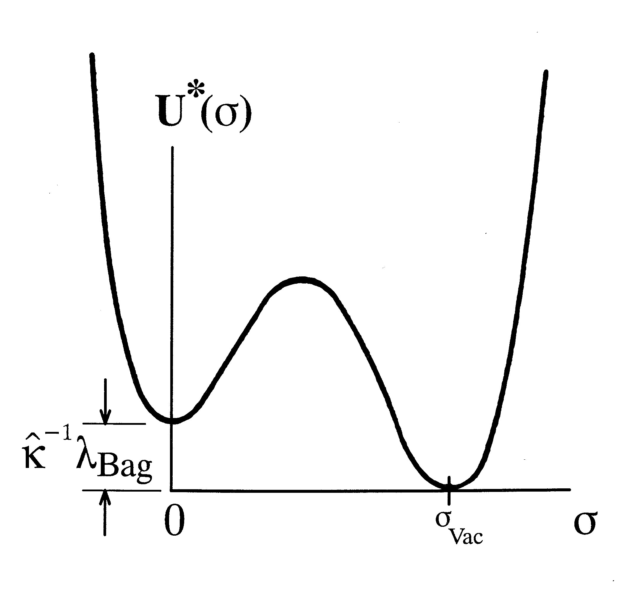
Figure 1: In the scalar-tensor model, the cosmological constant $\lambda\!=\!\lambda(\sigma)$ has two values because the scalar $\sigma$-field has undergone a phase transition and breaks the symmetry of the vacuum, creating two vacuum states. Inside the hadron, $\nu\!=<\!\sigma_{Bag}\!>=\!0$ and $\lambda\!=\!\lambda_{Bag}$, defining $\nu$ as $\nu\!\equiv<\!\sigma\!>$. Outside the hadron where $\nu\!=<\!\sigma_{Vac}\!>$, the gravitational ground-state energy density of the vacuum $E_{vac}$ is defined by the background metric $\eta_{\mu\nu}$ with $\lambda\!=\!\Lambda_{F-L}$ for the Friedmann-Lemaitre accelerating Universe. Both are a de Sitter space. The hadron bag constant $B\!=\!\hat{\kappa}^{-1}\lambda_{Bag}$ is the scale set by $U^{*}(\nu=0)$. Eq. (2.6) means that $\lambda\!=\!\hat{\kappa}U^{*}(\nu)$, or $\lambda_{Bag}\!=\!\hat{\kappa}B$ in the interior because $\nu\!=\!0$ there.

To introduce curvature in the vacuum, one defines gravity as $g_{\mu\nu}$ = $\eta_{\mu\nu}$ + $h_{\mu\nu}$. Necessarily the background $\eta_{\mu\nu}$ must be assumed (§1.2.2) in order to define the ground-state energy for classical gravity where there are no fluctuations ($h_{\mu\nu}=0$). Again, for this study that will be the accelerating F-L de Sitter space used in cosmology [63].
Now with reference to Figure 1, define $\nu\!\equiv\,<\!\sigma\!>$. The ground-state energy density occurs at the value $\nu\!=<\!\sigma_{vac}\!>=\!\nu_{vac}$. This corresponds to the VEV $E_{vac}(\nu_{vac})\!=\!U^{*}(<\!\sigma_{vac}\!>)\!=\!U^{*}(\nu_{vac})$, illustrated by the horizontal axis in Figure 1. It represents the nonperturbative QCD vacuum (1.15) external to the hadron in the presence of $\eta_{\mu\nu}$. This is the zero-temperature point where $h_{\mu\nu}$=0. Similarly at $\nu\!=0$, the VEV $E_{vac}(<\!\sigma\!>)=U^{*}(\nu\!=0)$ represents the perturbative vacuum (1.16) with bag constant $B=\hat{\kappa}^{-1}\lambda$, also illustrated in Figure 1. This figure portrays the scalar potential (1.5) used by Creutz [64] and others [65,66] in flat Minkowski space. Varying the parameters such as those of (1.5) [64], one can recover the basic bag model of [26] under certain limited circumstances.
Note that $\eta_{\mu\nu}$ is the F-L metric which includes the experimentally measured cosmological term $\Lambda_{F-L}$ $\sim$ $10^{-56}cm^{-2}$ corresponding to a vacuum energy density $(\sim 2\cdot 10^{-3}~{}eV)^{4}$. Next note that $E_{vac}$, the bag potential function $U^{*}(\sigma)$, and the value of $B=\hat{\kappa}^{-1}\lambda_{Bag}$ in $U^{*}(\sigma)$ are not observables. Also, $B$ is nonnegative.

2 The scalar-tensor model & hadron confinement

2.1 Summary of the Problem

Now we need a brief digression on Einstein gravity (1.1) and how to introduce $g_{\mu\nu}$ into hadron physics. The gravitational field equations (1.1) follow from the classical Einstein-Hilbert (E-H) action

$$S=-\frac{1}{2}\kappa^{-1}\!\int d^{4}x\sqrt{-g}(R-2\lambda)\quad.$$ (2.1)

where the associated Lagrangian is $\pounds_{EH}=\kappa^{-1}\sqrt{-g}(R-2\lambda)$, $g=det~{}g_{\mu\nu}$, and the slash in $\pounds$ means that $\sqrt{-g}\neq 1$ (i.e., it is not flat Minkowski spacetime). Typically in particle physics, the spacetime is flat, $\sqrt{-g}\rightarrow 1$, and Lagrangians are represented as $\mathfrak{L}$. Note that a term -​$\int d^{4}x\lambda$ in action (2.1) or -​$\int d^{4}xB$ in (1.11) is not invariant under coordinate transformations $x$ $\rightarrow$ $x^{\prime}(x)$. The presence of gravity plus Einstein’s principle assumption of general covariance or coordinate invariance regarding (1.1) and (2.1) requires that such a term be modified to $\int d^{4}x\sqrt{(-g)}\lambda$ in order that $\pounds$ behaves as a scalar and is a gauge invariant expression. As a result, $\pounds_{EH}$ becomes an infinite series in the metric (graviton) field $g_{\mu\nu}$ due to the presence of $\sqrt{-g}$ and $g^{\mu\nu}$ which is the inverse of $g_{\mu\nu}$, a property that does not happen in flat spacetime. In a weak-field expansion $g_{\mu\nu}$ = $\eta_{\mu\nu}$ + $h_{\mu\nu}$ about a space $\eta_{\mu\nu}$, one has [22]

$$\sqrt{(-g)}=1+\frac{1}{2}h_{\mu}^{~{}\mu}+\frac{1}{8}h_{\mu}^{~{}\mu}h_{\nu}^{~{}\nu}-\frac{1}{4}h_{\mu\nu}h^{\mu\nu}+O(h^{3})\quad.$$ (2.2)

This is not a cosmological term because it is dimensionless, but it illustrates what begins to happen in quantum gravity for an action (2.1) in curved spacetimes rather than flat space. Obviously, general covariance is broken when $\pounds\!\rightarrow\!\mathfrak{L}$.
To restore gravity to the theory of hadrons, several things are required. The first procedure is to introduce minimal coupling by requiring all Lagrangians $\mathfrak{L}\!\rightarrow\!\pounds$ while exchanging $g_{\mu\nu}$ for flat Minkowski metric terms such as in the electroweak theory $\mathfrak{L}_{EW}\!\rightarrow\!\pounds_{EW}$ of the SM $\mathfrak{L}_{SM}\!\rightarrow\!\pounds_{SM}$, and hadron theory $\mathfrak{L}_{NTS}\!\rightarrow\!\ \pounds_{NTS}$. Then with appropriate gravitationally covariant derivatives, general covariance is restored - which guarantees that Christoffel connections appear in the derivatives of (1.9) and (1.7) so that Yang-Mills gluons and spinors such as quarks will follow geodesics. To this, one adds the postulate of universal coupling [38] which amounts to Einstein’s principle of equivalence. The second, more serious step is the introduction of a scalar field, as already discussed in §1.2. The technique is developed in Appendix B [67-73].
Several things are already apparent about (2.1). First, it is notoriously nonrenormalizable in the conventional sense of QFT on curved backgrounds and quantum gravity because the Newtonian coupling constant G in $\kappa$ has a negative mass dimension (-2) in four dimensions. (1.1) and (2.1) are also intrinsically nonlinear and are not always subject to perturbative methods, much the same as for nonperturbative QCD.
Stelle [74] successfully showed that higher-order terms are in fact renormalizable, along with other researchers [75-80] as discussed in Appendix C for further reference [74-90]. However, the price one pays is loss of unitarity - noting that the only important example of a theory that is both renormalizable and unitary is $\mathfrak{L}_{SM}$ for the SM of particle physics, provided of course that the effects of gravity are not included.
In contrast to the higher-derivative approach of Stelle, a method of ghost-free gravitational Lagrangians has been found to re-establish unitarity by including terms quadratic in curvature as well as torsion [91]. Because of the spin vierbein connection in this technique, it may play a role in the unitarity of the Yang-Mills portion of QCD that follows here in (14). Nevertheless, a consistent theory of quantum gravity [22,23] or QFT has not yet been formulated (App. C.2) [81-90].
Summary Issue. Another issue about $\pounds_{EH}$ in (2.1) is that the vacuum energy density $\lambda$ in (2.1) and $B$ in (1.11) are two very different numbers. The problem here is to connect them in a genuine way. The first has mass-dimension two and the second four. Hence, there is an inconsistent dimensionality of the Lagrangians (1.13) and (2.1) regarding vacuum energy density. And again, introducing $B$ in (1.11) and $\lambda$ in (1) constitutes double counting which affects their renormalization loop equations. This will be fixed by identifying $\hat{\kappa}^{-1}\lambda$ in (2.1) as the first term of $U(\sigma)$ appearing in JFBD theory (Appendix B). That is, the bag is re-interpreted as a potential representing the cosmological term in gravitation theory.

2.2 Nonminimal coupling of quark bags with gravity

At the outset, quark confinement in the form of relativistic bags has one distinguishing feature as opposed to elementary particle theory. This feature even existed when the electron problem was posed in [2]. The bag is an extended, composite object subject to nonlocal dynamics. This has been pointed out by Creutz [64] while examining hadrons as extended objects for the bag model in [26]. Perturbation theory is not applicable. Hence in the presence of confinement, commonly accepted principles for point-like particles in QFT such as analyticity of scattering amplitudes are called into question. This must be kept in mind as a possible way around the loss of unitarity mentioned in §2.1 when strong fields are involved in nonlocal strong-interaction hadron physics. Unitarity may not be required or even possible for composite hadron models, although it might be restored using the ghost-free Lagrangian methods with torsion just mentioned, or by adopting the method in [92]. The Stelle Lagrangian in (B.1) of Appendix B.1 can replace (2.1) in this present report in a way that seems acceptable, recognizing that loss of unitarity continues to plague quantum gravity at this time.
In order to couple the NTS model in (1.6)-(1.14) with gravity, the total action for gravitation, matter, and gravitation-matter interaction is assumed to be

$$S=S_{Gravity}+S_{matter}+S_{G,m}\quad.$$ (2.3)

Matter will be limited to NTS ($\pounds_{m}$=$\pounds_{NTS}$), excluding the electroweak theory $\pounds_{EW}$ of the SM and the Higgs fields for this study. Nonminimal coupling will be used in the sense of scalar-tensor theory and the standard additional energy-momentum tensor $T_{~{}\mu\nu}^{\sigma}$ will be added for the $\sigma$-field, with details in Appendix B.
Transposing $\lambda$ to the right-hand side of (1.1) gives the scalar-tensor field equations

$$R_{\mu\nu}-\frac{1}{2}g_{\mu\nu}R=-\kappa T^{*}_{~{}\mu\nu}\quad,$$ (2.4)

$$T^{*}_{\mu\nu}=T^{M}_{~{}~{}\mu\nu}+T^{\sigma}_{~{}\mu\nu}\quad,$$ (2.5)

$$\lambda_{Bag}=\hat{\kappa}B\quad.$$ (2.6)

where now $\lambda=\lambda(\sigma)$ contributes to $T^{\sigma}_{~{}\mu\nu}$, the matter tensor is $T^{M}_{~{}~{}\mu\nu}=T_{\mu\nu}$ in (1.1), and $\kappa T^{*}_{~{}\mu\nu}$ is conserved by the Bianchi identities. We will derive (2.5) later [§2.3 and (B.35)]. (2.6) represents the new cosmological bag constant $B=\hat{\kappa}^{-1}\lambda$ introduced in this report. Unlike Einstein [2], we will use the traces $T^{M}=T^{M\mu}_{~{}\mu}$ and $T^{*}$ as two of several mechanisms to couple gravitation to the NTS $\sigma$-field of quantum bag theory.
Notice that the mass-dimension problem discussed in §2.1 has now been solved in (2.6). Both sides of this equation have mass-dimension two.
We want to determine $T^{\sigma}_{~{}\mu\nu}$ in (2.5) by introducing the self-interacting scalar potential $U(\sigma)$ and relating it to the origin of $\lambda_{Bag}$ in (2.6). The interaction term is $\pounds_{G,m}$=$\pounds_{G,\sigma}$. The Lagrangian for (2.3) now is

$$\pounds=\pounds_{NTS}+\pounds_{G}+\pounds_{G,\sigma}\quad,$$ (2.7)

where the original Einstein-Hilbert gravitation term $\pounds_{G}$ and the NTS contribution in (2.7) on a curved background are

$$\pounds_{G}=-\frac{1}{2}\kappa^{-1}R\quad,$$ (2.8)

$$\pounds_{NTS}=\pounds_{Q}+\pounds_{\sigma}+\pounds_{q,\sigma}+\pounds_{C}\quad,$$ (2.9)

with Higgs bosons and counter terms neglected. Eventually $\pounds_{\sigma}$ will be removed from (2.9) and made a part of $\pounds_{G,\sigma}$ in (2.7).
The critical matter-gravity interaction term $\pounds_{G,m}=\pounds_{G,\sigma}$ in (2.3) and (2.7) is viewed as the origin of $\lambda$ and conceivably hadron confinement. It is the symmetry breaking term.

2.3 The field equations (2.23) & (2.26)-(2.27)

In the conventional FLW bag model [19] with covariant derivatives, the quark $\psi$, scalar $\sigma$, and colored gluon $C$ terms originally in (1.6)-(1.14) now become (2.10)-(2.13) for use in (2.9)

$$\pounds_{q}=\bar{\psi}(i\gamma^{\mu}D_{\mu}-m)\psi\quad,$$ (2.10)

$$\pounds_{\sigma}=\frac{1}{2}\nabla_{\mu}\sigma\nabla^{\mu}\sigma-U(\sigma)\quad,$$ (2.11)

$$\pounds_{q,\sigma}=-f\bar{\psi}\sigma\psi\quad,$$ (2.12)

$$\pounds_{C}=-\frac{1}{4}\mathbf{\epsilon(\sigma)}\mathbf{F_{\mu\nu}F^{\mu\nu}}-\frac{1}{2}g_{s}\bar{\psi}\lambda^{c}A_{c}^{\mu}\psi\quad,$$ (2.13)

where $m$ is the quark flavor mass matrix, $f$ the $\sigma$-quark coupling constant, $g_{s}$ the strong coupling, $\mathbf{F_{\mu\nu}}$ the non-Abelian gauge field tensor, $D_{\mu}$ the gauge-covariant derivative, and $\nabla_{\mu}$ the gravitation-covariant derivative (also in $\mathbf{F_{\mu\nu}}$) with the spin connection derivable upon solution of (2.4), defining the geodesics. $\mathbf{\epsilon(\sigma)}$ is the phenomenological dielectric function introduced by Lee et al. [15], where $\epsilon(0)\!=\!1$ and $\epsilon(\sigma_{vac})\!=\!0$ in order to guarantee color confinement. The ${SU}_{3}$ Gell-Mann matrices and structure factors are $\lambda_{c}$ and $f_{abc}$.
Zel’dovich’s original argument [7,8] that the action (2.3) is a vacuum correction for quantum fluctuations led Sakharov [93] to expand the gravitational E-H Lagrangian $\pounds_{EH}$ in powers of the geometric curvature $R$

$$\pounds(R)=\pounds_{o}+\pounds_{G}(R)+\pounds(R^{2})+...\quad,$$ (2.14)

where $\pounds_{o}$ is the cosmological term and $\pounds_{G}$ is (2.8).
The positive contribution of matter and fields $\pounds_{m}$ in (2.3) is thereby viewed as offset by the negative contribution of gravitation and hence geometry in (2.14), a sort of back-reaction of the metric. We interpret $\pounds_{o}$ here as the spontaneous origin of the NTS $\sigma$-field whose nonlinear self-interaction breaks the symmetry of the vacuum and creates the bag ($B\neq 0$ in (1.11), (2.6), and Figure 1). The scalar-gravitation field coupling can take at least two zero- and first-order forms that relate to $T^{*}_{~{}\mu\nu}$ in (2.4) and (2.5),

$$\pounds_{G,\sigma}^{(0)}=-B\quad,$$ (2.15)

$$\pounds_{G,\sigma}^{(1)}=-\frac{d}{4}T^{*}\sigma\quad.$$ (2.16)

One can actually picture (2.15) and (2.16) as the first two polynomial terms of $\pounds_{o}$ in (2.14), by defining $U^{*}(\sigma)$ as $\pounds_{o}$

$$\pounds_{o}=-U^{*}(\sigma)\quad,$$ (2.17)

$$U^{*}(\sigma)=-\pounds_{G,\sigma}^{(0)}-\pounds_{G,\sigma}^{(1)}+U(\sigma)\quad$$ (2.18)

$$=B+\frac{d}{2}T^{*}\sigma+\frac{a}{2}\sigma^{2}+{\frac{b}{3!}}\sigma^{3}+{\frac{c}{4!}}\sigma^{4}\quad.$$ (2.19)

(2.18)-(2.19) contain the usual $U(\sigma)$ in (2.11), now linked to $g_{\mu\nu}$ in (2.4) via $T^{*}$ and $B$. The NTS Lagrangian $\pounds_{\sigma}$ in (2.11) can be re-defined to include $U^{*}(\sigma)$ instead of $U(\sigma)$,

$$\pounds^{*}_{\sigma}=\frac{1}{2}\nabla_{\mu}\sigma\nabla^{\mu}\sigma-U^{*}(\sigma)\quad,$$ (2.20)

$$=\pounds_{G,\sigma}\quad.$$ (2.21)

$\pounds_{\sigma}^{*}$ is $\pounds_{o}$ plus kinetic terms (momenta) built up from derivatives of $\sigma$. In (2.19), $a,b,c$ are adjusted to produce two minima (Figure 1), one at $\nu=0$ and one at a ground-state value $<\sigma_{vac}>=\nu_{vac}$, while fitting low-energy hadron properties [64-66,27,19]. The term $T^{*}\sigma$ is a chiral symmetry breaking term used to represent the cloud of pions surrounding the bag [66,94,95,19]. $d$ (along with $a,b,c$) adjusts this term by skewing (not tilting) the $U^{*}(\sigma)$ potential and breaking the $\sigma$ $\rightarrow$ $-\sigma$ symmetry.
This linear $\sigma$-term ($d\neq 0$) in (2.19) is not necessary to create the bag ($B\neq 0$), breaks dilatation invariance, and can be dropped ($d=0$). Furthermore, it breaks the renormalizability of $U(\sigma)$ in (1.11) by simple power counting of (2.16), $T^{*}$, and $\sigma$ as discussed in Appendix B, §B.5. If used, $d$ must be small enough to preserve the two minima in Figure 1, while slightly skewing the broken symmetry about the line $dT^{*}\sigma$. For $d=0$, then $U^{*}=U$.
Inspired by Sakharov in (2.14), $\pounds_{o}$ is the origin of $U^{*}(\sigma)$ and the $\sigma$-field. The term $\pounds_{\sigma}$ has been removed from (2.9) and placed in (2.20)-(2.21) and (2.17) as $\pounds_{\sigma}^{*}$, creating a scalar-tensor theory of gravitation via (2.3) and (2.7). Variation of (2.3), using (2.7)-(2.13) with (2.11) replaced by (2.20)-(2.21), gives the field equations (2.4) as well as those for $\sigma$ and $\psi$,

$$\square\sigma=U^{*\prime}(\sigma)+f\bar{\psi}\psi\quad,$$ (2.22)

$$(i\gamma^{\mu}D_{\mu}-m-f\sigma)\psi\quad,$$ (2.23)

if one neglects the gluonic contribution (2.13). $\square$ is the curved-space Laplace-Beltrami operator, and $U^{*\prime}=dU^{*}/d{\sigma}$ is

$$U^{*\prime}=\frac{d}{4}T^{*}+a\sigma+{\frac{b}{2}}\sigma^{2}+{\frac{c}{3!}}\sigma^{3}\quad.$$ (2.24)

A variant adopts $d=0$ to simplify (2.22) and (2.24) when pion physics is not involved.
The $T^{\sigma}_{~{}\mu\nu}$ contribution in (2.5), which can be improved [96], is

$$T^{\sigma}_{~{}\mu\nu}=\nabla_{\mu}\sigma\nabla_{\nu}\sigma-g_{\mu\nu}\pounds^{*}_{\sigma}\quad,$$ (2.25)

and is derived in Appendix B.2 as (B.35) and (B.47). (2.22) and (2.24) are a scalar wave equation for $\sigma$ whose Klein-Gordon mass, which is given in (B.38) and follows as (2.28), is $m_{\sigma}=\sqrt{a}$. Hence $\sigma$ is short-ranged and does not contribute to long-range interactions.
$T^{M}_{~{}~{}\mu\nu}$ in (2.5) is the quark and gluon contribution to the matter tensor, and $\kappa T^{\sigma}_{~{}\mu\nu}$ now contains (2.6). The trace of (2.5) is $T^{*}=T^{M}\sigma_{;a}^{2}+4U^{*}$, with traces for $T^{M}$, $T^{\sigma}$, and $T^{*}$ determined in Appendix B.2 and B.5.
The scalar-tensor model permits a number of options $\kappa=\kappa(\sigma)$, one of which is developed in Appendix B.2. There are four pertinent cases: (a) $\kappa(\sigma)$ = constant; (b) $\kappa(\sigma)=\sigma$; (c) $\kappa(\sigma)=\sigma^{-1}$; and (d) $\kappa(\sigma)$ arbitrary. (a) is Einstein gravity; (b) turns off $T^{*}_{~{}\mu\nu}$ in (2.4) [$\kappa(0)=0$] within the bag, leaving an Einstein space $R_{\mu\nu}=\lambda g_{\mu\nu}$ due to the cancellation $\kappa\kappa^{-1}\lambda_{Bag}=\lambda_{Bag}$; (c) is the ansatz originally used by Jordan-Fierz-Brans-Dicke [67-69]; and (d) $\kappa(\sigma)$ is any well-behaved function of $\sigma$ provided it results in consistent physics, a case that is not developed here (although it is discussed in Appendix B.4).
As derived in Appendix B.2 and (B.3) [67-72] following usual treatments, Case (c) gives for (2.25) and (2.22)

$$(R_{\mu\nu}-\frac{1}{2}g_{\mu\nu}R)=-\frac{8\pi}{\sigma}T^{M}_{\mu\nu}-\frac{\Omega}{\sigma^{2}}[\sigma_{;\mu}\sigma_{;\nu}-\frac{1}{2}g_{\mu\nu}\sigma_{;\alpha}\sigma^{;\alpha}]-\frac{1}{\sigma}[\sigma_{;\mu}\sigma_{;\nu}-g_{\mu\nu}\square\sigma]-\frac{1}{\sigma}g_{\mu\nu}U^{*}(\sigma)\quad,$$ (2.26)

$$\square\sigma=\frac{8\pi}{3+2\Omega}T^{*}+U^{*\prime}(\sigma)+f\bar{\psi}\psi\quad.$$ (2.27)

where $\Omega=(\kappa_{1}^{-1}-3/2)$, and $\kappa_{1}$ is the source of $\sigma$-coupling to the trace $T^{M}$ traditionally used in JFBD theory. $T^{M~{}~{};\nu}_{~{}~{}\mu\nu}=0$ is assumed in Case (c) (see [70] for an exception). $E(\sigma)$ is determined either by the Class A or B auxiliary constraints given in Appendix B.3. The Class A constraint is not renormalizable, while the Class B constraint determines $E(\sigma)=1$ by the argument surrounding (B.47).
In brief summary, the scalar field $\sigma$ in (2.27) is now coupled to the trace $T^{*}$ as opposed to (2.22). It represents an inverse gravitational constant $G^{-1}$ or coupling parameter $\kappa^{-1}=(8\pi G)^{-1}$ in (2.26), whose vacuum potential $U^{*}(\sigma)$ has two ground states that determine the vacuum energy density $\lambda(\sigma)$ in (2.6) and Figure 1. It is in this sense that gravitation couples to all physics, because of the ansatz in (B.3).

2.4 Consequences of the symmetry breaking

The field equations (2.26) and (2.27) are not the traditional JFBD problem in search for a Machian influence of distant matter or a time-varying $G$. (2.27) does not have a static solution $G^{-1}=\sigma\sim\Sigma m/r$ [97] because $\sigma$ has only short-range interaction by virtue of its mass $m_{\sigma}=\sqrt{a}$ in (B.38). To make the point, (2.27) can be re-written

$$(\square-m\sigma^{2})=\delta U^{*\prime}(\sigma)+\frac{8\pi}{3+2\Omega}T^{M}+f\bar{\psi}\psi\quad,$$ (2.28)

where $\delta U^{*\prime}$ is the remainder of (2.24) after moving the $a\sigma$ term to the left-hand side. Hence a static solution must have a Yukawa cutoff $\sigma\sim(e^{-\mu r})m/r$ where $\mu\sim m_{\sigma}$.
In addition, note carefully that (2.27) and (2.28) are totally absent from QCD in (1.6) - hence the need for a fundamental scalar boson beyond QCD for hadron theory.
It is true that $G$ is carried along as part of the JFBD method in Appendix B. However, the motivation for a $\sigma$-field coupled to gravitation in (2.27) is to try and solve the CCP, not investigate the origin of inertia.
There now exist two characteristic vacuum states for $\lambda(\sigma)\rightarrow U^{*}(\sigma)$ in Figure 1 governed by the field equations (2.4), (2.5), (2.19), and (2.26)-(2.27). These are

$$\lambda(<\sigma_{Bag}>)=\hat{\kappa}B\quad,$$ (2.29)

inside the hadron bag (1.16), and the “true” QCD vacuum $\nu_{vac}=<\sigma_{vac}>$ external to the hadron (1.15)

$$\lambda(<\sigma_{vac}>)\equiv\Lambda_{F-L}\quad,$$ (2.30)

scaled to the gravitational ground state $\eta_{\mu\nu}$ (de Sitter space).
As has been shown in Appendix A.1 for the weak-field limit of $g_{\mu\nu}$, the cosmological term $\lambda$ behaves as a graviton mass $m_{g}$ in (A.21)

$$m_{g}=\sqrt{2\Lambda_{F-L}/3}\quad,\qquad Hadron~{}Exterior$$ (2.31)

$$=\sqrt{2\lambda_{Bag}/3}\quad.\qquad Hadron~{}Interior$$ (2.32)

In terms of the gravitation constant $G$, using (2.6), the following are also true

$$m_{g}=\sqrt{16\pi G_{N}B/3}\quad,\qquad Hadron~{}Exterior$$ (2.33)

$$=\sqrt{16\pi G_{Bag}B/3}\quad.\qquad Hadron~{}Interior$$ (2.34)

The respective VEDs (2.29)-(2.30) and graviton masses $m_{g}$ (2.31)-(2.34) are summarized in Table I (§4).

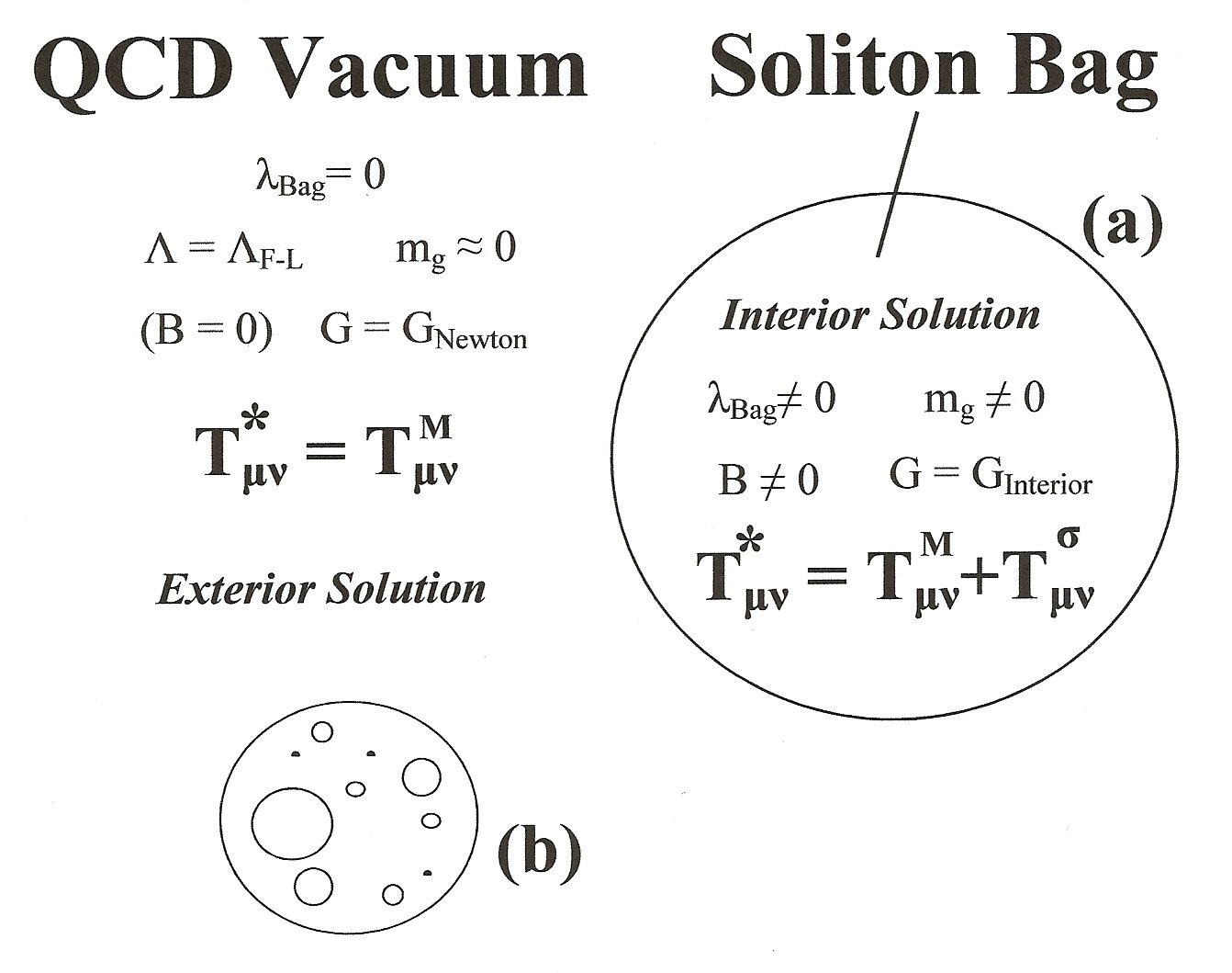
Figure 2: The existence of two vacuum states for $\lambda\!=\!\lambda(\sigma)$ results in both a short- and long-range gravitational force in hadron physics due to the connection between $\lambda$ and graviton mass $m_{g}$ in the weak-field approximation. The exterior is traditional Einstein gravity for an accelerating F-L Universe, except that the graviton has a tiny mass that cuts off at the Hubble radius. (a) A single soliton bag is depicted with a non-zero bag constant. For surface boundary conditions the following can be adopted: $F_{\mu\nu}n^{\nu}\!=\!0$ for gauge fields; and $\psi\!=\!0$ for quark fields. As a problem in bubble dynamics, one uses -$\frac{1}{4}$ $\bf{F}$^μν $\bf{F}$${}_{\mu\nu}\!=\!\Sigma J^{-1}\nabla_{\nu}(Jn^{\nu})\!+\!B$ for a quark current $J$ and surface tension $\Sigma$ [37, Hasenfratz & Kuti, p. 103]. Alternatively adopt the Lunev-Pavlovsky bag with a singular Yang-Mills solution on the bag surface [29,30]. (b) The general interior solution is depicted as a many-bag problem using a Swiss-cheese (Einstein-Straus) model of space-time with zero pressure on the bag surfaces.

Within the hadron bag. Here one has $m_{g}\neq 0$ due to (2.29) and (2.32). Adopting a simplified view of the hadron interior and a bag constant value from one of the conventional bag models, the MIT bag [26], $B^{1/4}=146~{}MeV$ or $B=60~{}MeVfm^{-3}$, then $\lambda_{Bag}=\hat{\kappa}B=2\cdot 10^{-3}~{}cm^{-2}$ from (2.6). Using (2.31)-(2.34), a graviton mass $m_{g}=3.7\cdot 10^{-7}cm^{-1}$ or $7.3\cdot 10^{-12}~{}eV$ is found within the bag. Although this appears to represent a Compton wavelength of $m_{g}^{-1}\sim 3\cdot 10^{6}~{}cm$ or range of $\frac{1}{2}m_{g}^{-1}\sim 1.5\cdot 10^{6}~{}cm$, it is derived from $\lambda_{Bag}$ and is only applicable for the interior solution. This is depicted in Figure 2. It has no range outside of the bag where $\lambda_{Bag}$=0.
A similar calculation for the Yang-Mills condensate $B_{YM}\sim 0.02~{}GeV^{4}$ [35] gives $\lambda_{YM}\sim 8.7\cdot 10^{-12}~{}cm^{-2}$ and $m_{g}\sim 2\cdot 10^{-6}~{}cm^{-1}$ or $4\cdot 10^{-11}~{}eV$, and $\frac{1}{2}m_{g}^{-1}\sim 2.5\cdot 10^{5}~{}cm$.
Regarding $G$, adopting $G_{Bag}=G_{Newton}$ is the conservative assumption to make. However, $G_{Bag}$ in (2.34) is a free parameter, independent of $B$. It has never been experimentally measured. For any $B$ determined in Table I of §4, $G_{Bag}$ can be anything except zero. It can re-scale the Planck mass, and therefore represents a new way of looking at the hierarchy problem (§4.4). Only experiment can determine its outcome.
External to the hadron. This is the nonperturbative QCD vacuum (1.15). By taking the well-known JFBD limit $\Omega\rightarrow\infty$ in (2.26)-(2.27), we in fact obtain Einstein gravity (for exceptions see [98]) due to the experimental limits given in §4. The small graviton mass $m_{g}$ in (2.31), on the other hand, results in a finite-range gravity whose mass is $m_{g}\sim 0.8\cdot 10^{-28}~{}cm^{-1}$ or $1.6\cdot 10^{-33}~{}eV$. This follows from the vacuum energy density ${\sim}$ $({{2\cdot 10^{-3}}~{}eV})^{4}$ which is equivalent to $\lambda\sim 10^{-56}~{}cm^{-2}$, for the de Sitter background $\eta_{\mu\nu}$ in the F-L accelerating Universe [63].
Obviously, $G=G_{Newton}$ in the exterior (Figure 2b).
Summary. The results are as follows. (2.31) gives a graviton mass $m_{g}\sim 0.8\cdot 10^{-28}~{}cm^{-1}$ and a range of $\frac{1}{2}m_{g}^{-1}\sim 6\cdot 10^{27}~{}cm$ which is approximately the Hubble radius. That is, gravitation within the bag is short-ranged, and gravitation outside of the bag is finite-ranged on the order of the Hubble radius. All of these cases are discussed further in §3 as how they relate to hadrons, and are summarized in §4 as how they relate to experiment.
Figure 2 depicts a single soliton bag embedded in the NTS-QCD gluonic vacuum (Fig. 2a), as well as for the many-bag, ”Swiss-cheese” model of spacetime [99] with bags-within-bags which results for multiple hadrons (Fig. 2b).
Clearly the sign of $\lambda$ must be positive (de Sitter space) in (2.31)-(2.34) in order that an imaginary mass not be possible. The latter represents an unstable condition with pathological problems such as tachyons and negative probability [41]. (2.31)-(2.34) is a physical argument against such a circumstance.

2.5 Finite temperature effects

The effect of finite temperature $T$ upon $U^{*}(\sigma)$ is treated in the usual fashion [100-102]. The classical, zero temperature potential $U^{*}(\sigma)$ becomes $V^{*}(\sigma)=U^{*}(\sigma)+V_{S}(\sigma,T)+V_{F}(\sigma,T,\mu)$ involving scalar $V_{S}$ and fermionic $V_{F}$ correction terms for chemical potential $\mu$, by shifting $\sigma$ as $\sigma=\sigma^{~{}\prime}+\nu(T)$. The result is a temperature-dependent cosmological bag parameter [103] $\lambda_{Bag}=\lambda_{Bag}(\mu,T)=\hat{\kappa}B(\mu,T)$ which decreases with increasing temperature $T$ until the bag in Figure 2 dissolves and symmetry is restored ($B=0$) in Figure 1.
In such a case and in simplest form [104], the bag model equations of state (EOS) are

$$\epsilon(T)=k_{SB}T^{4}+B\quad,$$ (2.35)

$$\ p(T)=k_{SB}T^{4}/3-B\quad,$$ (2.36)

$$k_{SB}=\frac{\pi^{2}}{30}(d_{B}+\frac{7}{8}d_{F})\quad,$$ (2.37)

where energy density $\epsilon$ and pressure $p$ now have a temperature dependence ($T\!\neq\!0$). The Stefan-Boltzmann (SB) constant $k_{SB}$ is a function of the degeneracy factors $d_{B}$ for bosons (gluons) and $d_{F}$ for fermions (quarks and antiquarks). The absence of the baryonic chemical potential $\mu$ in (2.35) is a valid approximation for ongoing experiments involving nucleus-nucleus collisions. (2.35)-(2.37) is relevant to quark-hadron phase transitions and the quark-gluon plasma (QGP).

3 Short-range gravitation and the hadron interior

So far the principal change has been to incorporate the bag constant of hadron physics into scalar-tensor gravitation theory, by treating the cosmological term in (1.1) and (2.6) as the potential function in (1.5), (2.5), (2.20), and (2.25). This has resulted in no significant experimental change in the hadron exterior.
The hadron interior, however, is a different matter. As depicted in Figure 1, $\lambda\rightarrow\lambda_{Bag}$ has now increased the VED there by 44 orders of magnitude. This is not to suggest that gravity per se can compete with strong interaction physics in QCD.⁵ What has changed is that gravity is necessarily involved in the Lagrangian $\pounds$ of action (2.3) while interacting with the NTS Lagrangian $\pounds_{NTS}$ (2.9) which includes QCD. Details of what gravity does under these circumstances have not appeared in the literature, and that is one of the purpose of this section (§3). Only if the gravitation constant $G_{interior}$ is experimentally measured to be significantly different than $G_{Newton}$ (§3.1.2 below) can these calculations play an important role in strong interaction physics.
Referring again to Figure 2, the hadron interior ($r\!<\!r_{Bag}$) is inhabited by quarks and gluons and is a de Sitter space with a constant $\lambda_{Bag}\neq 0$. These exist in the presence of a scalar field $\sigma(x)$ having mass $m_{\sigma}=\sqrt{a}$ in (B.38), and a graviton field $g_{\mu\nu}(x)$ of mass $m_{g}=\sqrt{2\lambda_{Bag}/3}$ in (2.32) whose helicities will be discussed later (§3.3.2). The physics of the quarks $\psi$ in (2.23) and gluon gauge fields $\mathbf{A^{\mu}}$ in (1.9) participate in the dynamics of bag excited states. Neither $\psi$ nor $\mathbf{A^{\mu}}$ exists in the external solution, with the bag surface behaving like that in the Lunev-Pavlovsky gluon-cluster model.
In the hadron exterior ($r\!>\!r_{Bag}$), nothing has really changed except for the tiny graviton mass (2.33) of $\sim\!10^{-33}eV$. This part of the problem has already been solved. By current experiments (§4), it is Einstein gravity about a charged or neutral hadron (with a Reissner-Nordström or Kottler-Schwarzschild solution) for a hadron mass $m_{h}$. The graviton mass cuts off at the Hubble radius. For most conceivable applications, it is negligible.
The bag per se ($r\leq r_{Bag}$) is governed by the short-range tensor field $g_{\mu\nu}(x)$ and short-range scalar $\sigma(x)$, their mutual interactions, the confined quarks $\psi$ and gluons $\mathbf{A^{\mu}}$, as well as the energy and pressure balance at the bag’s surface ($r\!=\!r_{Bag}$). Obviously there can be surface currents [37] that guarantee quarks and gluons do not exit the bag, as well as a bag thickness or skin depth $\delta$ where this takes place [e.g., 64]. Alternatively, the Lunev-Pavlovsky gluon-cluster model is equally possible. There also is a surface tension, since the nonperturbative QCD vacuum must offset the negative bag pressure created by $B$. All of these interactions are nonlinear and non-perturbative.
Finally, the complicated bag surface and thickness $\delta$ with boundary conditions need additional comment. It is important to observe that the zero pressure boundary condition (§3.1.1 and §3.3.2 below) is “free” - an automatic consequence of the phase transition in Figure 1 that created the bag. The bag constant $B$ is either $B\!=\!0$ or $B\!\neq\!0$, one of two states. Only when symmetry restoration is happening because $B\!=\!B(\mu,T)$ is actually temperature-dependent (§2.5), do more complicated dynamics come into play in the boundary condition problem.

3.1 Classical solutions for the field equations

Here are details addressing solutions for the equations of motion (2.23) and (2.26)-(2.27). Classical solutions may be useful in determining the consequences of the present investigation should experiment find that $G_{interior}$ has changed significantly as did $\lambda_{Bag}$,
Vacuum solutions of the original JFBD equations ($\lambda=0$) have been well investigated although all require quantum corrections [105]. The spherically symmetric static field for a point mass (with $c=1$)

$$ds^{2}=-e^{2\nu}c^{2}dt^{2}+e^{2\zeta}dr^{2}+r^{2}d\Omega^{2}$$ (3.1)

was first examined by Heckmann et al. [106] with later studies by Brans [107,68], Morganstern [108], Ni [109], Weinberg [69, pp. 244-248], and others [110]. Exact [107,111] static exterior and approximate [112,113] interior solutions have both been discussed, while exact rotating solutions that reduce to the Kerr solution when $\sigma\rightarrow 0$ have been found [114]. In addition, conformal transformations of solutions in Einstein gravity have been used to generate JFBD solutions [72]. Notably, the approximation [112,113] indicates that there are no singularities at $r=0$, the center of the sphere.

3.1.1 Boundary conditions in general

A generalized scalar-tensor theory has many similarities with the Kottler-Schwarzschild (KS) problem in Appendix A as far as boundary conditions are concerned. The obvious exception is that the scalar field $\sigma$ is regulated by a separate equation of motion (2.27)-(2.28) from the Ricci tensor $R_{\mu\nu}$ in (2.26). The $\sigma$-field is significant because without it there would be no bag and hence no multiple vacua. Excitations of $\sigma$ in (2.22), (2.23), and (2.24) couple to quark $\psi$ excited states in the hadron interior for modelling hadrons.
Spherical symmetry is assumed because it is a very good approximation to many physical situations. With that in mind, the goal is to establish that there exist interior solutions of the $\lambda$JFBD scalar-tensor theory assuming a perfect fluid whose pressure, mass density, metric, and scalar functions are everywhere finite in the bounded region of the hadron and have zero pressure $p=0$ at its surface.

3.1.2 Possible jump conditions

As discussed in §2.4, $G$, $B$, and $\lambda$ are now linked in a fundamental way, with only one restriction - relation (2.6). The two vacuum states in Figure 1 each have their own set of these basic parameters. There are no experimental short-range and strong-force measurements within a hadron that guarantee $G$ must equal Newton’s constant there. It is possible that $G\sim\kappa=\sigma^{-1}$ has two states with $G_{interior}$ being quite different from $G_{Newton}$ in the hadron exterior as depicted in Figure 2.
This has a direct consequence, related to the standard Einstein limit of JFBD gravity. One obtains Einstein gravity as the JFBD coupling constant $\Omega$ goes to infinity ($\Omega\rightarrow\infty$ with exceptions [98]) and $G\sim\kappa=\sigma^{-1}$ becomes constant. However, $G=constant$ does not mean that $G_{hadron}=G_{Newton}$ at the boundary condition interface between the interior and exterior solutions.
Hence, one must be cautious about $G$ in the interior and exterior solutions that follow and must await experimental measurements.

3.1.3 Energetics and boundary conditions for the bag

When Einstein introduced $\lambda$ into physics, he created a negative pressure $p$ represented by $B\neq 0$ in Figure 1, that is

$$p=-B\quad.$$ (3.2)

The energy-momentum tensor $T_{\mu\nu}$ for a bag is then

$$T_{\mu\nu}=(\rho-B)u_{\mu}u_{\nu}-Bg_{\mu\nu}\quad,$$ (3.3)

where $\rho$ is the mass density introduced by quarks and gluons, and $u_{\mu}$ is the 4-velocity of the assumed isotropic, homogeneous, incompressible perfect fluid in the interior. The latter is not spatially flat. It is a de Sitter space with $R=4\lambda_{Bag}$ containing $N_{q}$ quarks, at least in the Einstein limit $\Omega\rightarrow\infty$ of (2.26) and (2.27).
For comparison, consider the bag from the point of view of hadron physics. Also treat it as spherical and static. All quarks are in the ground state, as opposed to a compressible bag [115]. Figure 2 represents a simple hadron containing $N_{q}$ quarks. In its simplest form, the hadron mass $M_{h}$ for bag volume $V=4\pi r^{3}/3$ is [115]

$$M_{h}=kV^{-1/3}+BV\quad,$$ (3.4)

where on the right-hand-side the first term is the internal quark energy and the second is the volume energy. The volume is determined by pressure balance between the internal quarks and the external QCD pressure, as

$$\frac{\partial M_{h}}{\partial V}=-\frac{1}{3}kV^{-4/3}+B\quad.$$ (3.5)

$k$ and $B$ are found from experimental values for the proton charge radius and a given nucleon mass. From (3.4) and (3.5), one has for the static bag

$$V=(k/3B)^{3/4}\quad,$$ (3.6)

$$M_{h}=4(k/3)^{3/4}B^{1/4}\quad.$$ (3.7)

Dynamically, boundary conditions are established on the surface of the bag in order that the quarks and gluons cannot get out (since free quarks have not been observed). Then hadrons are viewed as excitations of quarks and gluons inside the bag. Confinement is achieved phenomenologically (inserted by hand) in the MIT bag [26] by requiring that there is no quark current flow through the surface of the bag (Figure 2, caption). This results in a nonlinear boundary condition which breaks Lorentz invariance. A similar requirement will be assumed here for examining preliminary solutions, rather than address the Lunev-Pavlovsky gluon-cluster model at this time.
The boundary condition generates discrete energy eigenvalues $\epsilon_{n}$ for the quarks where

$$\epsilon_{n}=c_{n}/r\quad,$$ (3.8)

and $c_{1}=2.04$ for the ground state $n=1$. Assuming that $N_{q}$ is the number of quarks inside the bag, then their kinetic energy is $E_{kin}=N_{q}\epsilon_{n}$ while the potential energy $E_{pot}$ is $E_{pot}=BV$. $E_{pot}$ must be subtracted from the total bag energy $E$ in order to obtain the total quark energy

$$E-BV=N_{q}c_{1}/r\quad.$$ (3.9)

3.1.4 Special case classical solutions

The specific results for the classical solutions are presented in Appendix D [116-123].

3.2 The weak-field versus strong-field limit

It has been shown in Appendix A that for the weak-field limit of $g_{\mu\nu}$ in §A.1, the cosmological term $\lambda$ behaves as a graviton mass $m_{g}=\sqrt{2\lambda/3}$ in (A.21). We have not shown, however, that $\lambda$ behaves as a graviton mass in the strong-field case. See the caution given regarding (A.15). Certainly with higher-derivative and renormalizable Lagrangians such as (B.1) or (B.2), it needs to be demonstrated for very strong gravitational fields that the $m_{g}$ term in (A15) still survives as a graviton mass.
Higher derivatives, viewed as momenta, portray high energy and therefore high temperatures. From §2.5, symmetry restoration must eventually set in and the bags dissolve or disappear.

3.3 The strong-field case

3.3.1 Historical background

The early 1970’s witnessed a sophisticated revival of the old search for unification that dates back to Mie [1] and Weyl [3]. For example, Freund introduced a Brans-Dicke scalar [120] with unification in mind following an earlier investigation of finite-range gravitation [121].
It also was suggested by Salam et al. [124-125] and independently Zumino [126] that hadrons interact strongly through the exchange of Spin-2 mesons behaving as tensor gauge fields. The Salam group adopted a bi-metric theory of gravity by adding a second set of Einstein equations (1.1) for a new tensor field $f_{\mu\nu}$ that would mix with the usual $g_{\mu\nu}$, producing what they called $f\!-\!g$ gravity. The $f_{\mu\nu}$ field described a Spin-2 particle ($f$-meson) bearing a Pauli-Fierz mass [56] similar to the method of [126].
Two cosmological constants were introduced, one for the $f$-field and one for the $g$-field. Hadrons were described as two superimposed de Sitter microuniverses that interacted through $f\!-\!g$ mixing. These are very similar to present-day multiverses or metaverses. Unlike QFT, Einstein’s theory offers no founding principles upon which to define interactions in an $f\!-\!g$ multi-tensor system. So such a scheme is contrived at best. This is a fact that plagues any multi-metric theory. Metrics must be imbedded using appropriate boundary conditions as in Einstein-Straus [99], not superimposed.
$f\!-\!g$ gravity had a lot of problems and fell into disfavor. Deser [127] established many of the difficulties associated with Spin-2 mixing. Aichelburg [128] showed it was impossible to construct a bi-metric tensor gravity theory in the same spacetime without losing causality. The concept of causal metrical structure breaks down due to the existence of two propagation cones. It was also shown that there exist too many intractable Spin-2 helicities (seven and eight) [128,129]. And Freund [120] showed that the experimentally observed $f$-mesons were not the quanta of a gauge field of strong gravity.
As a matter for historical perspective, the gravitation theory presented here was found quite independently of multi-metric theories. It was arrived at while trying to solve the CCP.

3.3.2 Mass and Spin-2 graviton degrees of freedom

Attributing a graviton mass to the region of confinement, the hadron bag, necessarily brings up old problems originating at the beginning of quantum gravity (Appendix C). The issue is how to reconcile a graviton mass with the interior of a hadron bag.
Pauli-Fierz Method. The traditional method for introducing a graviton mass in Spin-2 quantum gravity is that of Pauli-Fierz [56] because it does not introduce ghosts and its Spin-0 helicity survives in the massless limit, naturally leading to a JFBD scalar-tensor theory of gravitation [52]. Unfortunately, the Pauli-Fierz mass $m_{PF}$ is derived from quantum gravity arguments for massive particles having integral Spin-2 on a flat background $\eta_{\mu\nu}$. As with Veltman [41], this is simply incorrect [42] if Einstein gravity is the experimentally correct one (§4). Pauli & Fierz focus on Lorentz invariance and positivity of energy after quantization. However, they totally ignore the cosmological constant ($\lambda=0$), and its association with graviton mass in the weak-field limit (Appendix A). The conventional way of working around this oversight is to introduce the Pauli-Fierz mass term as a weak-field perturbation $g_{\mu\nu}$ = $\eta_{\mu\nu}$ + $h_{\mu\nu}$ on a curved background $\eta_{\mu\nu}$ which is de Sitter space ($\lambda\neq 0$) [58] instead of a flat Minkowski space as they assumed for quantum gravity.
vDVZ Discontinuity. Later, the subject of finite-range gravitation resulted in the realization of what is known as the vDVZ discontinuity [130,131,132,52]. In the linear approximation to Einstein gravity using the Pauli-Fierz mass term (App. §A.2), the zero-mass limit of a massive graviton does not result in the same propagator as the zero-mass case. The consequence is that giving a nonzero mass $m_{g}=m_{PF}$ to a graviton results in a bending angle of light near the edge of the Sun that is 3/4 that of Einstein’s value, and the difference may be measurable [52]. This quantum gravity dilemma is discussed in [131]. Its resolution is making $m_{g}$ small enough and not using perturbative approximations [133]. That is accomplished here in the hadron exterior where the free graviton has a tiny mass and a range on the order of the Hubble radius.
As for the interior, there is no bending of light experiment that can be performed inside a hadron bag (§4). Hence, the vDVZ discontinuity is not relevant to the short-range modification of Einstein gravity presented here, because there is no massless limit inside a hadron (Figure 2) where $\lambda_{Bag}$ cannot be zero and $m_{PF}$ is not introduced. In fact, the fundamental premise of the scalar-tensor theory is that quantum symmetry breaking has resulted in a finite discontinuity in Figure 1 between the two vacua. This results in two discontinuous values of $\lambda$ and one can even conjecture that a similar thing happens to $G$ (§3.1.2). A difference in graviton propagators inside and outside the bag is to be expected, cautioning that propagators are derived from perturbative Feynman techniques that cannot reflect the nonperturbative physical properties of confinement and strong interactions. Again [133], the vDVZ discontinuity appears to be an artifact of perturbation theory.
A key point is that hadron bags are composite objects. Some physical behavior that applies to elementary particle physics may not apply to hadrons. Recalling the suggestion of Creutz [64] that certain fundamental concepts such as unitarity may be called into question when discussing composite systems, it may be time to ask similar questions about the graviton degrees of freedom inside a hadron bag. Ultimately the question is how to deal with loss of unitarity in a still undefined quantum gravity, and how to admix the boson (scalar, gluon, and graviton) degrees of freedom consistently.
Helicity Properties in the Exterior. Recalling the summary for (A.20) of Appendix A.2, the result is a well-behaved massive graviton generated by $\lambda$ with two transverse helicities obtained in the weak-field approximation. The Spin-0 component is suppressed by coupling to a zero-trace $T^{M}\!=\!0$ energy-momentum tensor while the vector Spin-1 components are eliminated by using the gauge $f_{\mu}\!=\!0$ in (A.8). That method is applicable here in the hadron exterior (2.31).
Helicity Properties in the Interior. For the interior (2.31), the same technique can be applied except that one does not suppress the Spin-0 component because this couples to the $\sigma$-field constituting the bag in scalar-tensor theory (recall §1.3.1, [62]). This appears as coupling to the trace $T^{M}\!\neq\!0$ in (2.27). Similarly, one argues that the vector degrees of freedom for Spin-1 couple to the Yang-Mills gauge gluon fields of QCD - without need for the gauge $f_{\mu}=0$ in (A.8).
All five degrees of freedom appear necessary for confinement, although as few as four have been discussed under other circumstances [57]. The $\sigma$-field and the gluons conceptually can interact with $g_{\mu\nu}$ in such a way as not to lose unitarity within the bag - but that appears impossible to prove in the nonperturbative environment of confinement with no consistent theory of quantum gravity and no experimental data.

4 Experimental prospects

In this study a $\lambda$-generated graviton mass (2.31)-(2.34) has appeared, with different values inside and outside the hadron. For the case inside the hadron, that will be referred to as the confined graviton. That outside will be called the free graviton. The free graviton has a mass $\sim\!10^{-33}eV$ ($\Lambda_{F-L}\!\neq\!0$) with a range extending to the Hubble radius since it is scaled to the vacuum energy density $({{\sim\!2\cdot 10^{-3}}eV})^{4}$ or $\lambda_{F-L}\sim\!10^{-56}cm^{-2}$ characterizing the F-L accelerating Universe [63, Blome & Wilson]. In addition, the scalar gluon (condensate) $\sigma$-field has acquired a mass $m_{\sigma}\!=\!\sqrt{a}$ (B.38). The $\sigma$-field comprises the hadron bag as a composite object, and represents the cosmological term as a potential (§B.1) in scalar-tensor gravitation theory, (2.3)-(2.6).

Table 1: Summary of the masses, vacuum energy densities (VED s), and $\lambda\text{'}$s in spacetime. The QCD vacuum (1.15) scales to the VED of accelerating F-L cosmology, with a graviton mass whose range is approximately the Hubble radius.

Spacetime	$m_{g}$	$m_{g}$	$m_{\sigma}$	VED,$B$	$\lambda$
Region	$(cm^{-1})$	$(eV)$	$(GeV)$	$(GeV)^{4}$	$(cm^{-2})$
Hadron Exterior
$\lambda\equiv\Lambda_{F-L}\neq 0$	0.8x$10^{-28}$	1.6x$10^{-33}$		2x$10^{-47}$	0.7x$10^{-56}$
Hadron Interior
MIT bag [26]	3.7x$10^{-7}$	7.3x$10^{-12}$	$\sqrt{a}$	$0.0045$	2x$10^{-13}$
Y-M cluster [35]	2.4x$10^{-6}$	4x$10^{-11}$	$\sqrt{a}$	$0.02$	9x$10^{-12}$

These two principal features, a graviton mass and a scalar gluon mass, are summarized in Table I. Both have experimentally observable consequences. Basic experimental findings and limitations are discussed below in §4.1 and §4.2, while experimental consequences for the $\sigma$-field mass $m_{\sigma}$ are given in §4.3. Those for the graviton mass $m_{g}$ are addressed in §4.4 and §4.5. And finally, recent developments in the dilepton channels of jets at Fermilab are related to a possible scalar gluon condensate in §4.6.

4.1 Einstein gravity as correct long-range theory

Einstein’s theory of gravitation is remarkably successful on long-distance scales, along with its low-energy Newtonian limit based upon the inverse-square law at short distances. This has been verified over the range from binary pulsars to planetary orbits and short-distances on the order of 1 mm [134,135,38]. That conclusion is arrived at experimentally using spacecraft and lunar orbital measurements [136], as well as terrestrial laboratory tests of the inverse-square law (ISL) [137,138], and the principle of equivalence [134].
Similarly, Einstein gravity has prevailed experimentally over the JFBD scalar-tensor theory for the same distance scales. Experimental limits on the JFBD parameter $\Omega$ from planetary time-delay measurements place it at best as $\Omega\geq 500$ while Cassini data indicates it may be $\Omega\geq 40,000$ [139]. For practical purposes, this is approximating the limit $\Omega\rightarrow\infty$ when one examines the PPN parameter $\gamma$ in solutions given in Appendix D, Case (a.2) where $\gamma\rightarrow 1$ in (D.8). Further JFBD limits have been found in cosmology [139,Wu & Chen; Weinberg].
This means that JFBD theory is basically Einstein gravity with $\gamma\rightarrow 1$. But these two theories are not equivalent, as shown here, because $\sigma$ is significantly related to $\lambda$ which in turn is the source of the CCP in Einstein gravity (§1.1). In fact, it is $\sigma$ that helps solve the CCP.
In this context, no gravitational theory has been experimentally verified at the scales and energies that are the focus of the present study, and now follow below. Hence, Einstein gravity ($\Lambda=0$) still prevails as the correct theory of gravity for all energies presently subject to experiment. The present study does not change that well-established fact.

4.2 Issues in and below the sub-millimeter regime

At short-distances scales below $1~{}cm$, the issue of what to measure is an entirely different matter. There are virtually no experimental constraints on gravitational behavior at this range of interaction.
This scale eventually becomes the realm of hadron and high-energy particle physics. It is the realm that transitions from classical gravity to quantum gravity. And it must address the physics of confinement per se because the graviton may play a pertinent role in that process.
Conventional Methods. The first experimental issue is the method of parameterization for identifying new forces and effects. At the $mm$-scale, this is usually a comparison with a short-range Yukawa contribution to the familiar ISL $1/r^{2}$ term [137], as

$$V(r)=-V_{o}[1+\alpha e^{-r/\lambda^{\prime}}]$$ (4.1)

where $V_{o}$ is the ISL term, $\alpha$ is a dimensionless parameter, and $\lambda^{\prime}$ is a length scale or range. The data are then published as graphs of $\mid\!\alpha\!\mid$ versus $\lambda^{\prime}$ [138]. It can be said that the ISL is valid down to $1~{}mm$ [137].
Limitations of Conventional Techniques. At these scales traditional experiments using torsion-balance or atomic microscopy techniques for studying the ISL, begin to encounter a strong background of nongravitational forces. These include the Casimir and van der Waals forces [140]. Price [141] has pointed out that the experimentally accessible region for ISL study is limited to ranges greater than $40~{}\mu m$ by the electrostatic background force created by the surface potentials of metals and other materials.
Experimental Quantum Gravity (EQG). Given that there is no consistent renormalizable theory of quantum gravity, there seems to have been little or no experimental work in quantum gravity at the short-distance scale.
In anticipation of the Large Hadron Collider (LHC) now operating at CERN, there has been much written about the onset of EQG at the TeV scale. This includes dilatons and moduli from string theory, the leaking of gravitons into extra dimensions, M-theory, lowered Planck scales, and so forth. Most are attempts to solve the SM hierarchy problem [137].

4.3 Experimental consequences for scalar gluon mass

One of the first things to observe about the SM in particle physics is that it seems to ignore the scalar bag in hadron physics. To see this, simply note that $\pounds_{SM}=\pounds_{EW}+\pounds_{QCD}+\pounds_{Int.}$ does not include any of the $\sigma$ terms in (2.7), (2.9), or (2.10)-(2.13). If there is anything observable about $\sigma$ and the hadron bag, the SM is going to miss it. Bag theory is apparently categorized as physics beyond the SM although no one seems to have pointed this out.
It is QCD that couples to the $\sigma$-field in (1.13) and (1.14). Hence it is QCD that the present scalar-tensor theory must reckon with. Since this study adopts the FLW NTS confinement model from the outset, its compatibility with QCD in the strong coupling regime has already been demonstrated [15,17,19,142].
What is new is the distinctive feature of the $\sigma$-field as a nonlinear, self-interacting scalar that represents the gluon condensate (or scalar gluon [18]) associated with hadron confinement (a bag), a broken symmetry in the QCD vacuum, the bag constant $B$, and Einstein’s cosmological constant $\lambda$. This scalar $\sigma$-field has a classical mass $m_{\sigma}=\sqrt{a}$ in (B.38) and is a boson. As mentioned in §1.3.1, it couples attractively to all hadronic matter in proportion to mass. Hence, the $\sigma$-field has now become a fundamental field in scalar-tensor gravitation theory.
Note that the wave equation in (2.27) for $\sigma$ couples to the trace $T^{M}$ with mass contributions from the quark condensates $f\bar{\psi}\psi$ ($f\!\neq\!0$). (2.27) states that the scalar gluon (condensate) $\sigma$ is observable as an exchange force. It makes predictions as to how $\sigma$ interacts with the quark condensates and all matter.
However, this does not mean that the bag is an observable in the laboratory. Under high-temperature (§2.5) collisions, the bag can bifurcate or dissolve entirely (e.g., hadron decay). The ultimate EQG question is whether the mass of the $\sigma$-field is a directly measurable quantity, much akin to measuring the gluon condensate in a free state which may include a quark-gluon plasma. In another vein, the bag potential function $U(\sigma)$ or $U^{*}(\sigma)$ is not an observable.
So how can one determine $m_{\sigma}=\sqrt{a}$ ?
The mass $m_{\sigma}$ appears in all bag interaction potentials (2.19) either via SSB or when inserted by hand (such as Klein-Gordon or Pauli-Fierz). In order to derive the mass $m_{\sigma}$ for comparison with experiment, it depends upon the parameterization of $U^{*}(\sigma)$ in (2.19). There, the parameters $a,b,c$ (following the FLW NTS model) are interrelated and are used in conjunction with the bag constant $B$ to characterize a given hadron. As an alternate choice, Creutz [64] uses $\alpha,\beta,\gamma$ and $B$. To these, one adds $f$ in (2.12) and the strong coupling constant $\alpha_{s}=g_{s}/4\pi$ from (2.13). In any case, based upon the characteristics defining confinement, one uses these parameters to construct $U^{*}(\sigma)$ and model the hadron at every level of approximation possible [19, pp. 21-22; 142], including temperature.
The answer, then, is that one takes the observed boson mass $m_{\sigma}$ and defines a in the confinement potential, as $a=m_{\sigma}^{~{}2}$. That is one experimental observable that contributes to the definition of $U^{*}(\sigma)$, from which hadron dynamics (e.g. excited states) can be analyzed and predictions made.

4.4 Experimental consequences for graviton mass inside the hadron

As for the subject of graviton mass, physics has yet to detect a graviton at all [134] much less at the EQG scale of short-distance gravitation. The EQG-scale confined graviton appears undetectable, much like the neutrino. Hence its properties must be determined from things with which it interacts. It also sheds most of its mass if a confined graviton emerges from the disintegrating hadron bag, shifting its mass $m_{g}$ from (2.32) to (2.31).
Nevertheless, inside the hadron the confined graviton acquires a mass via (2.32) and is shown in Table I. As with all of the discussions of graviton physics at LHC energies mentioned above, an obvious thing to look for in exchange interactions is missing energy plus jets. If graviton propagators are transporting energy and they cannot be detected, then this must show up as a missing energy.
As an example, for the case of direct graviton production in say $p\bar{p}\rightarrow jet+graviton$, some have conjectured missing energy signatures [143]. However, for the graviton in Table I, the mass of a freed graviton is no longer (2.32) but rather (2.31) with a range that can reach a Hubble radius. It is virtually massless at $\sim\!10^{-33}eV$.
In practice, it is difficult to tell experimentally the difference between quarks and gluons. The reason is that both particles appear in the jets of hadrons [144]. Confined graviton propagation may be even more difficult and much more tedious.
Finally, the graviton mass relation in (2.34) states that for a given vacuum energy density $B$ in the hadron interior ($B$=constant), the gravitational coupling constant $G$ does not have to be the Newtonian one in the exterior (§3.1.2). Since $G$ has never been experimentally determined in quantum gravity at sub-$mm$ scales, this is an important effect that needs to be addressed. Changing $G_{Interior}$ moves the Planck scale in the interior. If one moves the scale of the Planck mass ($M_{Pl}=1/\sqrt{G}$) , how is $G$ measured and determined? One can consider this as a means for studying the SM hierarchy problem: Increase $G$. However, how can it be proven experimentally? The strategy is that the gravitational effects predicted in (2.26)-(2.27) can be made more significant by substantially increasing $G$, thus increasing the confined graviton mass (2.34) and spacetime curvature ($R=4\lambda_{Bag}$) inside the hadron. If those effects are experimentally established, then the issue is resolved. Note that the excited state (the bag) at $<\sigma>=0$ does not change when modifying $G$ because $B$ is assumed (above) to be a constant.
If the Planck mass is moved significantly, the weak-field approximation of Appendix A is no longer valid. The subject must then address the strong-field gravitational case which is beyond the scope of this study and quantum gravity as we understand it.

4.5 Prospects in astrophysics and cosmology

A graviton mass has direct relevance to gravitational radiation research in astrophysics and cosmology [134,135]. This is important because gravitational wave astronomy is destined to become one of the new frontiers in our understanding of the Universe.
The bound on graviton Compton wavelength $m_{g}^{-1}$ derived for gravitational-wave observations of inspiralling compact binaries [135,38] is $m_{g}^{-1}\!\sim\!6\cdot 10^{17}~{}cm$. From Table I, the Compton wavelength of a free graviton is $m_{g}^{-1}\!\sim\!10^{28}~{}cm$ which is eleven orders of magnitude safely beyond this experimental constraint. A similar comparison applies to the velocity of graviton propagation. Likewise, strong-field gravitational effects in stellar astrophysics (where Einstein gravity is known to prevail) are similarly unaffected by the small numbers in Table I for the free graviton mass.

4.6 Implications of Fermilab dilepton channel data about jets

The dilepton channel data observed at Fermilab [145] warrants comment from the point of view of hadron bag physics (§4.3 above). During $p\bar{p}$ collisions at $\sim 2~{}TeV$, an unexpected peak has been found centered at $144~{}GeV/c^{2}$ during the production of a W boson which decays leptonically in association with two hadronic jets.
This could be a signal of a scalar gluon $\sigma$-field as discussed in §4.3 during the production of jets. If such a case proves plausible ($m_{\sigma}=144~{}GeV/c^{2}$), then $a=m_{\sigma}^{2}=2.07\cdot 10^{4}~{}GeV^{2}/c^{4}$ in the hadron potential $U^{*}(\sigma)$ for the hadrons involved.
However, it is well-known that annihilation energy (such as $e\bar{e}$ and $p\bar{p}$) can re-materialize into vector and scalar gluon jets [146]. Hence much additional work, involving the LHC, needs to address this subject.

5 Comments and conclusions

5.1 Summary

A scalar-tensor theory of gravitation has been introduced as a modified Jordan-Fierz-Brans-Dicke model involving a scalar $\sigma$-field used in bag theory for hadron physics. The two vacua (1.15) and (1.16), illustrated in Figure 1, have a natural explanation as a hadron inflated by a negative bag pressure $B$ in the gravitational ground-state background $\eta_{\mu\nu}$ of an accelerating Friedmann-Lemaitre (de Sitter) Universe. These results follow from having made the simple observation that the cosmological term $\lambda$ in Einstein gravity is a scalar potential function (§B.1) and represents the confinement potential $U^{*}(\sigma)$ in $\pounds^{*}_{\sigma}$ (2.20) of hadron bag theory. Since the $\sigma$-field in turn represents the gluon condensate (or gluon scalar [18]) in QCD as a scalar field, it is straight forward to conclude that scalar-tensor theory is a natural choice for introducing gravity - albeit weak or strong - into particle physics at the TeV scale.
This scalar gluon couples to all hadronic matter uniformly, resulting in an attractive force proportional to hadron mass. Hence it is a gravitational interaction.
Lee’s original motivation [18] for introducing the $\sigma$-field was to treat it as a phenomenological field that describes the collective long-range effects of QCD. There it has no short-wavelength components, so the $\sigma$-loop diagrams can be ignored leaving only tree diagrams. That is, $\sigma$ has been regarded as a quasi-classical field.

5.2 Postulates

Eight postulates or principal assumptions have been used, as follows:

1. The classical Einstein-Hilbert Lagrangian is augmented by a nonminimally coupled scalar NTS term $\pounds_{NTS}$ in the fashion of JFBD theory. The $\pounds_{NTS}$ term represents hadron physics which includes QCD as $\pounds_{QCD}$ in the exact limit $\pounds_{NTS}\rightarrow\pounds_{QCD}$.

2. The gravitational field $g_{\mu\nu}$ couples minimally and universally to all of the fields of the Standard Model, as does Einstein gravity. However, $g_{\mu\nu}$ also couples minimally and nonminimally to the composite features of hadron physics $\pounds_{NTS}$, not just $\pounds_{QCD}$. This entails hadron physics.

3. General covariance is necessary in order to define the procedure for the use of the Bianchi identities in determining conservation of energy-momentum from $T^{M}_{~{}~{}\mu\nu}$ in (2.5). That means matter follows Einstein geodesics and obeys the principle of equivalence. This assumption can be broken, applying the Bianchi identities to $T^{*}_{~{}\mu\nu}$ instead. In such a case, the theory changes. Also, use of the harmonic gauge (Appendix A) gives rise to a graviton mass, but breaks general covariance.

4. Quantum vacuum fluctuations result in a broken vacuum symmetry, producing two distinct vacua containing two different vacuum energy densities $\lambda$. Because $\lambda=\lambda(\mu,T)$, this broken symmetry is subject to restoration.

5. The stability of the bag is assured by the vacuum energy density $B$ which is a negative vacuum pressure.

6. The relation between graviton mass $m_{g}$ and $\lambda(\mu,T)$ found in the weak-field approximation, survives in the strong-field and strong-force cases.

7. The NTS Lagrangian $\pounds_{NTS}$ is renormalizable. The E-H Lagrangian $\pounds_{EH}$ is not, but it can be extended and made renormalizable at the sacrifice of unitarity. Using the argument that unitarity is not required for the interiors of composite objects such as hadrons, this is less of a problem. The expansion of the Lagrangian used here to include the additional terms of (B.1) then produces a tenable, renormalizable model for hadron physics that includes gravitation provided there is no chiral symmetry breaking ($d\!=\!0$). Deviation from unitarity, however, may signal the onset of new physics [147].

8. The CCP has arisen because of inconsistent double-counting of $\lambda$ as a vacuum energy density both in QFT and in Einstein gravity - and with inconsistent dimensionality.

5.3 Conclusions

Until now, a tensor theory with both short- and long-range gravitation has not been devised. It has been shown in the weak-field approximation that this theory has both finite-range and short-range confined gravitational fields. The short-range gravitational field is only present inside the hadron while gravity outside the hadron involves a free graviton possessing a tiny mass that reaches to the Hubble radius. A guiding principle has been that gravity is universally coupled to all physics. Hence that must include the composite features of hadron physics as well.
What emerges is a conceivable confinement mechanism for the hadron bag that involves gravity. In previous work, the bag was introduced ad hoc into flat-space using a Heaviside step function, or was explained with Lee’s color dielectric continuum model and Wilets extension of it. Here, however, gravitation is the origin of the vacuum energy density and is coupled directly to the scalar gluon (condensate) in QCD.
Finally, the study indicates that unification is another motivation for examining scalar-tensor theory in particle physics. As shown in §4, these results are consistent with everything that is experimentally well established in QCD and Einstein gravity.

6 Acknowledgments

The author would like to acknowledge communications with O.V. Pavlovsky and S.J. Aldersley.

Appendix A The cosmological constant as a graviton mass

It was shown some time ago by this author [40] that the cosmological term $\lambda$ in General Relativity can be interpreted as a graviton mass, a result that will be reviewed in this Appendix. Veltman subsequently [41] made a similar conclusion, except for Spin-2 quantum gravity - pointing out that the associated graviton propagators have negative probability. However, Veltman’s result is not equivalent to what will be discussed here because he “abandons from the start things like curved space.” Spin-2 quantum gravity in flat space and quantized Einstein gravity are not the same thing since the latter is nonlinear and notoriously nonrenormalizable. Christensen & Duff [42] have emphasized that quantizing Spin-2 gravity with $\lambda\neq 0$ must not be carried out by expansion in flat space, contrary to Veltman’s results. One must consistently expand about a curved background field that satisfies the Einstein equations (1.1) with a $\lambda$ term. There is also no compelling reason for singling out de Sitter space from the multitude of classical solutions where $\lambda\neq 0$.
The question, then, is to examine what is going on in General Relativity. Is or is not $\lambda$ in (1.1) equivalent to or related to a graviton of non-zero rest mass in the sense of a wave equation? Some say yes [43-45] while others say no [46-48] or declare that a graviton mass is impossible [49]. Note with caution that an unqualified graviton mass is beset with numerous problems in QFT.

A.1 Weak-field limit, Kottler-Schwarzschild metric

The curved background adopted here will be a Kottler-Schwarzschild (KS) metric with $\lambda\neq 0$ [50] applied to the Regge-Wheeler-Zerilli (RWZ) problem [51] of gravitational radiation perturbations produced by a particle falling onto a large mass $M^{*}$. The Einstein field equations (1.1) are repeated below for convenience:

$$R_{\mu\nu}-\frac{1}{2}g_{\mu\nu}R+\lambda g_{\mu\nu}=-\kappa T_{\mu\nu}\quad.$$ (A.1)

One considers a small perturbative expansion of (A.1) about a known exact solution $\eta_{\mu\nu}$ subject to the boundary condition that $g_{\mu\nu}$ becomes $\eta_{\mu\nu}$ as $r\!\rightarrow\!\infty$. The metric tensor $g_{\mu\nu}$ is thus assumed to be $g_{\mu\nu}$ = $\eta_{\mu\nu}$ + $h_{\mu\nu}$ where $h_{\mu\nu}$ is the dynamic perturbation such that $h_{\mu\nu}<<\eta_{\mu\nu}$ = $g_{\mu\nu}^{(0)}$. By virtue of Birkhoff’s theorem [52], the most general spherically symmetric solution is well-known to be a KS metric

$$ds^{2}=-e^{\nu}dt^{2}+e^{\zeta}dr^{2}+r^{2}d\Omega^{2}\quad,$$ (A.2)

where

$$e^{\nu}=1-\frac{2M}{r}-\frac{\lambda}{3}r^{2}=e^{-\zeta}\quad,$$ (A.3)

while $M=GM^{*}/c^{2},d\Omega^{2}=(d\theta^{2}+\sin^{2}\theta d\phi^{2})$, and $\eta_{\mu\nu}$ is determined from (A.1) as $\eta_{\mu\nu}=diag(-e^{\nu},e^{-\nu},r^{2},r^{2}\sin 2\theta)$ in spherically symmetric coordinates ($r,\theta,\phi$). Its contravariant inverse is $\eta^{\mu\nu}$ defined as $\eta_{\mu\nu}\eta^{\mu\nu}=\delta_{\mu}^{\nu}$. Note that when $M^{*}\!=\!0$ in (A.1) a de Sitter space results and photons following geodesics do not travel at the speed of light $c$. Hence $\lambda\neq 0$ implies a photon rest-mass [40,53]. Although this geometric property of curved backgrounds has been often ignored by gauge theorists, it does not mean disaster for gauge invariance. Goldhaber & Nieto [54] have provided a very nice discussion of the fact that Stueckelberg’s construction [55] removes the formal gauge-invariance argument for a zero photon mass (and certainly for curved backgrounds). Gauge invariance does not forbid an explicit mass term for the gauge field should the graviton be the gauge boson.
The wave equation for gravitational radiation $h_{\mu\nu}$ on the non-flat background containing $\lambda$ in (A.1) follows as (A.20) below, derived now from the formalism developed for studying the RWZ problem. Perturbation analysis of (A.1) for a stable background $\eta_{\mu\nu}=g_{\mu\nu}^{(0)}$ produces the following

$$[h_{\mu\nu;\alpha}^{\quad~{};\alpha}-h_{\mu\alpha;\nu}^{\quad~{};\alpha}-h_{\nu\alpha;\mu}^{~{}\quad;\alpha}+h_{\alpha~{};\mu;\nu}^{~{}\alpha}]+\eta_{\mu\nu}[h_{\alpha\gamma}^{~{}~{};\alpha;\gamma}-h_{\alpha~{};\gamma}^{~{}\alpha~{};\gamma}]+h_{\mu\nu}(R-2\lambda)-\eta_{\mu\nu}h_{\alpha\beta}R^{\alpha\beta}=-2\kappa~{}\delta T_{\mu\nu}.$$ (A.4)

Stability must be assumed in order that $\delta T^{\mu\nu}$ is small. This equation can be simplified by defining the function (introduced by Einstein himself)

$$\bar{h}_{\mu\nu}\equiv h_{\mu\nu}-\frac{1}{2}\eta_{\mu\nu}h$$ (A.5)

and its divergence

$$f_{\mu}\equiv\bar{h}_{\mu\nu}^{~{}~{};\nu}\quad.$$ (A.6)

Substituting (A.5) and (A.6) into (A.4) and re-grouping terms gives

$$\bar{h}_{\mu\nu;\alpha}^{\quad~{};\alpha}-(f_{\mu;\nu}+f_{\nu;\mu})+\eta_{\mu\nu}f_{\alpha}^{~{};\alpha}-2\bar{h}_{\alpha\beta}R^{\alpha~{}~{}\beta}_{~{}\mu\nu}-\bar{h}_{\mu\alpha}R^{\alpha}_{~{}\nu}-\bar{h}_{\nu\alpha}R^{\alpha}_{~{}\mu}$$ (A.7)

$$+h_{\mu\nu}(R-2\lambda)-\eta_{\mu\nu}h_{\alpha\beta}R^{\alpha\beta}=-2\kappa\delta T_{\mu\nu}\quad.$$

Now impose the Hilbert-Einstein-de Donder gauge which sets (A.6) to zero

$$f_{\mu}=0\quad,$$ (A.8)

and suppresses the vector gravitons. ($f_{\mu}\neq 0$ can be retained for further simplification in some cases of $\eta_{\mu\nu}$, although problematic negative energy states may be associated with these vector degrees of freedom.) (A.8) now reduces wave equation (A.7) to

$$\bar{h}_{\mu\nu;\alpha}^{\quad~{};\alpha}-2\bar{h}_{\alpha\beta}R^{\alpha~{}~{}\beta}_{~{}\mu\nu}-\bar{h}_{\mu\alpha}R^{\alpha}_{~{}\nu}-\bar{h}_{\nu\alpha}R^{\alpha}_{~{}\mu}-\eta_{\mu\nu}h_{\alpha\beta}R^{\alpha\beta}+h_{\mu\nu}(R-2\lambda)=-2\kappa~{}\delta T_{\mu\nu}\quad.$$ (A.9)

In an empty ($T_{\mu\nu}=0$), Ricci-flat ($R_{\mu\nu}=0$) space without $\lambda$ ($R=4\lambda=0$), (A.9) further reduces to

$$\bar{h}_{\mu\nu;\alpha}^{\quad~{};\alpha}-2R^{\alpha~{}~{}\beta}_{~{}\mu\nu}\bar{h}_{\alpha\beta}=-2\kappa~{}\delta T_{\mu\nu},$$ (A.10)

which is the starting point for the RWZ formalism.

A.2 Weak-field limit, de Sitter metric

Since $\lambda\neq 0$ is of paramount interest here, we know that the trace of the field equations (A.1) gives

$$4\lambda-R=-\kappa T$$ (A.11)

whereby they become

$$R_{\mu\nu}-\lambda g_{\mu\nu}=\kappa[T_{\mu\nu}-\frac{1}{2}g_{\mu\nu}T]\quad.$$ (A.12)

For an empty space ($T_{\mu\nu}=0$ and $T=0$), (A.12) reduces to de Sitter space

$$R_{\mu\nu}=\lambda g_{\mu\nu}\quad$$ (A.13)

and the trace (A.11) to

$$R=4\lambda\quad.$$ (A.14)

Substitution of (A.13) and (A.14) into (A.9) using (A.5) shows that the contributions due to $\lambda\neq 0$ are now of second order in $h_{\mu\nu}$. Neglecting these terms (particularly if $\lambda$ is very, very small) simplifies (A.9) to

$$\bar{h}_{\mu\nu;\alpha}^{\quad~{};\alpha}-2R^{\alpha~{}~{}\beta}_{~{}\mu\nu}\bar{h}_{\alpha\beta}=-2\kappa~{}\delta T_{\mu\nu}\quad.$$ (A.15)

Note that one can arrive at (A.15) to first order in $h_{\mu\nu}$ by using $g_{\mu\nu}$ as a raising and lowering operator rather than the background $\eta_{\mu\nu}$ - a result which incorrectly leads some [48] to the conclusion that $\lambda$ terms cancel in the gravitational wave equation.
Furthermore, note with caution that (A.15) and the RWZ equation (A.10) are not the same wave equation. Overtly, the cosmological terms have vanished from (A.15), just like (A.10) where $\lambda$ was assumed in the RWZ problem to be nonexistent in the first place. However, the character of the Riemann tensor $R^{\alpha\mu\nu\beta}$ is significantly different in these two relations.
Let us simplify the KS metric by setting the central mass $M^{*}$ in $\eta_{\mu\nu}$ to zero. This produces the de Sitter space (A.13)-(A.14) of constant curvature $K=1/R^{2}$, where we can focus on the effect of $\lambda$. The Riemann tensor is now

$$R_{\gamma\mu\nu\delta}=+K(g_{\gamma\nu}g_{\mu\delta}-g_{\gamma\delta}g_{\mu\nu})$$ (A.16)

and reverts to

$$R^{\alpha~{}~{}\beta}_{~{}\mu\nu}=+K(g^{\alpha}_{~{}\nu}g_{\mu}^{~{}\beta}-g^{\alpha\beta}g_{\mu\nu})$$ (A.17)

for use in (A.15). This substitution (raising and lowering with $\eta_{\mu\nu}$) into (A.15) now gives a $K$ and a $\lambda$ term contribution

$$-2K[(\bar{h}_{\mu\nu}-\eta_{\mu\nu}\bar{h})+(\bar{h}_{\alpha\mu}h^{\alpha}_{~{}\nu}+\bar{h}_{\nu\beta}h^{\beta}_{~{}\mu}-\bar{h}h_{\mu\nu}-\eta_{\mu\nu}h^{\alpha\beta}\bar{h}_{\alpha\beta})]+\lambda[2\bar{h}_{\mu\alpha}h^{\alpha}_{~{}\nu}+\eta_{\mu\nu}h_{\alpha\beta}^{2}]$$ (A.18)

to second order in $h_{\mu\nu}$. Recalling that curvature $K$ is related to $\lambda$ by $K=\lambda/3$, substitution of (A.18) back into (A.15) gives to first order

$$\bar{h}_{\mu\nu;\alpha}^{\quad~{};\alpha}-\frac{2}{3}\lambda\bar{h}_{\mu\nu}+\frac{2}{3}\lambda\eta_{\mu\nu}\bar{h}=-2\kappa~{}\delta T_{\mu\nu}\quad.$$ (A.19)

There is no cancellation of the $\lambda$ contributions to first order. Noting from (A.5) that $\bar{h}=h(1-\frac{1}{2}\eta)$, then a traceless gauge $\bar{h}=0$ means either that $h=0$ or $\eta=2$. Since $\eta=4$, (A.19) reduces to

$$\bar{h}_{\mu\nu;\alpha}^{\quad~{};\alpha}-\frac{2}{3}\lambda\bar{h}_{\mu\nu}=-2\kappa~{}\delta T_{\mu\nu}$$ (A.20)

in a traceless Hilbert-Einstein-de Donder gauge where $\bar{h}_{\mu\nu}^{~{}~{};\nu}=\!0$ and $\bar{h}_{\mu}^{~{}\mu}=\!0$. (A.20) is a wave equation involving the Lapace-Beltrami operator term $\bar{h}_{\mu\nu;\alpha}^{~{}\quad;\alpha}$ for the Spin-2 gravitational perturbation $\bar{h}_{\mu\nu}$ bearing a mass

$$m_{g}=\sqrt{2\lambda/3}\quad,$$ (A.21)

similar to the Klein-Gordon equation $(\square-m^{2})\phi=0$ for a Spin-0 scalar field $\phi$ in flat space.
Summary. Because the trace $T$ was assumed to vanish in step (A.13)-(A.14), the scalar graviton (since it couples to $T\!\neq\!0$) has been suppressed along with the two vector Spin-1 components by virtue of the gauge condition $f_{\mu}\!=\!0$, leaving only two transverse degrees of freedom of the $(2S\!+\!1)\!=\!5$ helicities for a massive graviton. One can study further expansions of (A.20) to show that the $\lambda$ term survives but this has been done elsewhere [40].
Hence a well-behaved massive graviton containing two transverse degrees of freedom has been obtained without ghosts (preserving unitarity) in the weak-field approximation. This has been accomplished by not introducing the traditional Pauli-Fierz [56] mass term $\mathfrak{L}_{PF}=\frac{1}{4}m_{PF}^{2}(h_{\mu\nu}h^{\mu\nu}\!-\!h^{\mu~{}2}_{~{}\mu})$ which is often described as the only ghost-free form for a Spin-2 particle [52]. Spin-2 graviton ghost problems can also be averted by beginning with a scalar-tensor theory [13, Duff] as is done in this study.
Note that general covariance has been broken by going to the Hilbert-Einstein-De Donder gauge $f_{\mu}\!=\!0$ in (A.8) in order to suppress the vector gravitons. Note also that radiation reaction is a direct dividend of the nonlinear Einstein theory which is not accounted for in the linearization used by the RWZ- or KS-formalism employed here.
Finally, Duff et al. [57] have corroborated the results presented here that $m_{g}\!=\!\sqrt{2\lambda/3}$ in (2.31)-(2.32), as well as Higuchi [58] save for a factor of two.

A.3 Conformal invariance and mass

As a sanity check, consider the following. Penrose [59] showed that the zero rest-mass free-field equations for each spin value are conformally invariant if interpreted suitably. For a massless Spin-0 field $\phi$ on a background with scalar curvature $R$, the wave equation is

$$(\square-\frac{R}{6})\phi\quad,$$ (A.22)

a result that can be generalized to arbitrary integer spin [60]. According to the Klein-Gordon equation $(\square-m^{2})\phi\!=\!0$ for such a field in flat space, one concludes that $\phi$ has a mass $\!m=\!\sqrt{R/6})$. For the graviton case (A.20) in the previous section, substituting (A.14) or $R\!=\!4\lambda$ into (A.22) represents a de Sitter space whereby

$$(\square-\frac{2}{3}\lambda)\phi=0\quad.$$ (A.23)

We have recovered precisely the weak-field wave equation (A.20), except as the Spin-0 component of a graviton with the same mass $m_{g}\!=\!\sqrt{2\lambda/3}$.

Appendix B Scalar-tensor theory with Jordan-Fierz-Brans-Dicke ansatz

B.1 Fundamentals of scalar-vector-tensor theory

The prevailing theory of gravitation is Einstein gravity (§4) whose Lagrangian (2.1) provides the field equations (1.1). It is a scalar-vector-tensor theory in which its field tensor $g_{\mu\nu}$ consists of sixteen independent variables that interact through the energy-momentum tensor $T_{\mu\nu}$ with other fields. $T_{\mu\nu}$ is comprised of a Spin-2 (tensor), three Spin-1 (vectors), and two Spin-0 (scalars) admixtures totaling 16 degrees of freedom or helicities. By assuming symmetry $T_{\mu\nu}=T_{\nu\mu}$ two of the Spin-1 (vector) admixtures are suppressed. Energy conservation $T_{\mu\nu}^{~{}~{};\nu}=0$ eliminates the remaining vector and one of the scalars. The final scalar can be removed by ensuring that there is no trace ($T_{\mu}^{~{}\mu}\!=\!0$) which can interact with $g_{\mu\nu}$. The result is a well-behaved, consistent, massless graviton in its quantum gravity version.
The Lagrangian is used to bring the above dynamics together. Ideally, there might be one scalar field $\phi$, one vector field $A_{\mu}$ such as Yang-Mills or Maxwell or both, and the graviton that work together in a unified fashion. Since the focus here is on the scalar field contribution in curved backgrounds, we can discuss a generic Lagrangian using three simple scalar densities: $\sqrt{-g}R$, $\sqrt{-g}\mathfrak{B}$, and $\sqrt{-g}$ where $\mathfrak{B}$ represents any of the Lorentz scalar interactions allowable under the inhomogeneous group discussed in Appendix C.2, although many of these can be introduced by simply re-defining the covariant derivative $\nabla_{\mu}$ in the sense of gauge invariance. Noting that there must also be a kinematic term for the gradient of the scalar field $\phi$, an example of such a general Lagrangian in four dimensions is as follows:

$$\pounds=\sqrt{-g}[f_{1}(\phi)R+f_{2}(\phi)\mathfrak{B}+f_{3}\nabla_{\mu}\phi\nabla^{\mu}\phi-\lambda(\phi)]\quad,$$ (B.1)

recognizing that $\phi(\lambda)\sqrt{-g}$ is the cosmological term and is a function of the scalar field $\phi$. It actually is a scalar potential function $\lambda(\phi)=U(\phi)$ which determines the vacuum energy density. Since Lagrangians $\pounds=T-U$ are kinetic energy ($T$) minus potential energy ($U$), (B.1) can be also written

$$\pounds=\sqrt{-g}[f_{1}(\phi)R+f_{2}(\phi)\mathfrak{B}+f_{3}\nabla_{\mu}\phi\nabla^{\mu}\phi-U(\phi)]\quad.$$ (B.2)

To the right-hand-side must be added the source term for matter $\pounds_{matter}$ that produces $T_{\mu\nu}$ . This discussion is the general idea for the scalar portion of the scalar-tensor theory and what follows in Appendix B. One can see that the nonlinear $\sigma$-field Lagrangian $\pounds_{\sigma}$ for the bag in (2.11) and (2.20) appears naturally in the right-hand-side of (B.2).

B.2 Basic derivations in support of field equations (2.26)-(2.27)

In its original form, JFBD theory [67,68] did not include a potential $U(\sigma)$ or $\lambda$. The E-H action (2.1) was used with $\lambda\!=\!0$. Since the theme of the present study is $\lambda$ with major emphasis on the $\lambda\!=\!\lambda(\phi)$ term in (B.1), although with the substitution $\phi\!\rightarrow\!\sigma$ representing the scalar $\sigma$-field, the scalar-tensor theory must be modified (denoted as $\lambda$JFBD).
JFBD made the assumption that the reciprocal of Newton’s gravitational coupling constant $G^{-1}$ is to be replaced by a scalar field $\sigma$. This is known as the JFBD ansatz:

$$\kappa=\sigma^{-1}$$ (B.3)

which is adopted here because this is how scalar-tensor theory began. It needs to be noted that $\kappa\!\rightarrow\!\kappa(\phi)$ can be any permissible function of the scalar field provided this results in consistent physics. A non-permissible example would a polynomial of degree $n\!=\!5$ including $\sigma^{5}$ in (1.11) which by dimensional counting would result in dimensional coefficients that produce a nonrenormalizable potential $U^{*}(\sigma)$. See §B.3 for more.
The $\lambda$JFBD Lagrangian $\pounds_{\lambda JFBD}$, assuming (B.3) and including a kinetic term for $\sigma$ while re-instating potential $U^{*}(\sigma)$ and $\lambda$, is then

$$\pounds_{\lambda JFBD}=\frac{1}{2}\sqrt{-g}[-\sigma R+\frac{\Omega}{\sigma}\nabla_{\mu}\sigma\nabla^{\mu}\sigma-U^{*}(\sigma)]+8\pi\pounds_{matter}$$ (B.4)

where $\Omega$ is the dimensionless JFBD coupling constant. (B.4) is basically an extension of the Jordan-type action in [67]. Once again, it has been modified by the presence of a vacuum energy density potential $U^{*}(\sigma)$. Variation $\delta S=0$ of (2.3) using (B.4) gives the field equations for $g_{\mu\nu}$ and $\sigma$ to be derived below.
The energy-momentum tensor in (2.5) is comprised of two terms: $T^{*}_{~{}\mu\nu}=T^{M}_{~{}\mu\nu}+T^{\sigma}_{~{}\mu\nu}$. First is the usual matter contribution $T^{M}_{~{}\mu\nu}$

$$T^{M}_{~{}~{}\mu\nu}=\frac{2}{\sqrt{-g}}[\frac{\partial(\sqrt{-g}\pounds_{M})}{\partial g^{\mu\nu}}-\partial^{\alpha}\frac{\partial(\sqrt{-g}\pounds_{M})}{\partial(\partial^{\alpha}g^{\mu\nu})}]$$ (B.5)

which includes all matter fields in the Universe except gravitation, and it is assumed to be independent of the $\sigma$-field.
Characteristic of the JFBD theory, there is a new term $T^{\sigma}_{~{}\mu\nu}=\nabla_{\mu}\sigma\nabla_{\nu}\sigma-g_{\mu\nu}\pounds^{*}_{\sigma}$ which must include the effects of $\pounds_{G,\sigma}$ in (2.18). Consolidating all of the $\sigma$ terms and introducing a superscript R for renormalizable, we have in short-hand derivative notation

$${}^{R}T^{\sigma}_{~{}\mu\nu}=\sigma_{;\mu}\sigma_{;\nu}-\frac{1}{2}g_{\mu\nu}\sigma_{;}^{\alpha}\sigma_{;\alpha}+g_{\mu\nu}U^{*}(\sigma)\quad.$$ (B.6)

With (B.5) and (B.6), variation of (B.4) will give the final result (2.26)-(2.27) in the text as shown below.
A principal assumption follows Brans and Dicke. One does not want to sacrifice the success of the principle of equivalence in Einstein’s theory [38]. Hence only $g_{\mu\nu}$ and not $\sigma$ enters the equations of motion for matter consisting of particles and photons. The interchange of energy between matter and gravitation thus must follow geodesics as assumed by Einstein [69]. Therefore, the energy-momentum tensor (B.5) is assumed to be conserved in the standard fashion, $T^{M~{}~{};\nu}_{~{}~{}\mu\nu}\!=\!0$ (for exceptions see Footntes (9) and (11), as well as [70]). This also places an important constraint on the Spin-2 degrees of freedom in the quantized version.
Now it is time to focus on $T^{\sigma}_{~{}\mu\nu}$ in (B.6). The most general symmetric tensor of the form (B.6) which can be built up from terms each of which involves two derivatives of one or two scalar $\sigma$-fields, and $\sigma$ itself, is

$$T^{\sigma}_{~{}\mu\nu}=A(\sigma)\sigma_{;\mu}\sigma_{;\nu}+B(\sigma)\delta_{\mu\nu}\sigma_{;\alpha}\sigma^{;\alpha}+C(\sigma)\sigma_{;\mu;\nu}+D(\sigma)\delta_{\mu\nu}\square\sigma+E(\sigma)g_{\mu\nu}U^{*}(\sigma)\quad.$$ (B.7)

We want to find the coefficients $A,B,C,D,$ and $E$. One can make the argument that the last term in (B.7) is $g_{\mu\nu}U^{*}(\sigma)$, whereby $E(\sigma)\equiv 1$ (§B.3), but we will carry $E(\sigma)$ along at the present time.
Recalling that

$$\nabla_{\mu}U(\sigma)=\frac{dU^{*}}{d\sigma}\frac{d\sigma}{d\mu}\equiv U^{*\prime}(\sigma)\sigma_{;\mu}\quad,$$ (B.8)

the covariant divergence of (B.6) is

$${}^{R}T^{\sigma~{}\mu}_{\quad~{}\nu;\mu}=\sigma_{;\nu}\square\sigma-\sigma_{;~{};\nu}^{\mu}\sigma_{;\mu}+U^{*\prime}(\sigma)\sigma_{;\nu}\quad,$$ (B.9)

and the covariant divergence of (B.7) is

$$T^{\sigma~{}\mu}_{~{}\quad\nu;\mu} ~{}= \quad[A(\sigma)+B^{\prime}(\sigma)]\sigma_{;}^{\mu}\sigma_{;\nu}\sigma_{;\mu}{}$$ (B.10)

$${}+[A(\sigma)+D^{\prime}(\sigma)]\sigma_{;\nu}\square\sigma{}$$

$${}+[A(\sigma)+2B(\sigma)+C^{\prime}(\sigma)]\sigma_{;~{};\nu}^{\mu}\sigma_{;\mu}{}$$

$${}+[D(\sigma)](\square\sigma)_{;\nu}{}$$

$${}+[C(\sigma)]\square(\sigma)_{;\nu}){}$$

$${}+[E(\sigma)U^{*\prime}(\sigma)+U^{*}(\sigma)E^{\prime}(\sigma)]\sigma_{;\nu}\quad.$$

Multiplying the field equations (2.4) and (2.5) by $\sigma$, one obtains

$$(R_{\mu\nu}-\frac{1}{2}g_{\mu\nu}R)\sigma=-8\pi T^{M}_{~{}~{}\mu\nu}-8\pi T^{\sigma}_{~{}\mu\nu}\quad.$$ (B.11)

Taking the divergence of (B.11) gives

$$(R_{\mu\nu}-\frac{1}{2}g_{\mu\nu}R);^{\mu}\sigma+(R_{\mu\nu}-\frac{1}{2}g_{\mu\nu}R)\sigma_{;}^{\mu}=-8\pi T^{M~{}~{}\mu}_{~{}\mu\nu;}-8\pi T^{\sigma~{}~{}\mu}_{~{}\mu\nu;}\quad.$$ (B.12)

The first term on the left-hand-side of (B.12) is zero by virtue of the Bianchi identities. The first term on the right-hand-side is zero because $T^{M~{}~{};\nu}_{~{}~{}\mu\nu}\!=\!0$ and is conserved in order that matter follows Einstein geodesics (principle of equivalence). Next turning to an identity involving the Riemann tensor $R^{\gamma}_{~{}\alpha\nu\beta}$, first and second derivatives of a covariant vector $A^{\gamma}$ contain an antisymmetric part [69]

$$A^{\gamma}_{~{};\nu;\beta}-A^{\gamma}_{~{};\beta;\nu}=A^{\alpha}R^{\gamma}_{~{}\alpha\nu\beta}\quad.$$ (B.13)

This relation (B.13) means the first non-zero term in (B.12) is

$$R_{\mu\nu}\sigma_{;}^{\mu}=\sigma^{~{}\alpha}_{;~{};\alpha;\nu}-\sigma^{~{}~{}\alpha}_{;\nu;~{};\alpha}=(\square\sigma)_{;\nu}-\square(\sigma_{;\nu})\quad.$$ (B.14)

Taking the trace of (2.4) and (2.5)

$$R=\kappa T^{M}+\kappa T^{\sigma}\quad$$ (B.15)

and using the equation of motion for $\sigma$ (with $\sigma$-quark coupling constant $f=0$) to include the gravitational coupling to the trace $T^{M}$ of Einstein gravity,

$$\square\sigma=\frac{1}{2}\kappa_{1}T^{M}+U^{*\prime}(\sigma)\quad$$ (B.16)

$$T^{M}=2\kappa_{1}^{-1}(\square\sigma-U^{*\prime}(\sigma))\quad.$$ (B.17)

From (B.7) we obtain the other trace

$$T^{\sigma}=[A(\sigma)+4B(\sigma)]\sigma^{;\alpha}\sigma_{;\alpha}+[C(\sigma)+4D(\sigma)]\square\sigma+4[E(\sigma)U^{*}(\sigma)]\quad.$$ (B.18)

It follows from (B.15), (B.16), and (B.18) that

$$R=2\kappa_{1}^{-1}(\square\sigma+U^{*\prime}(\sigma))+\kappa([A(\sigma)+4B(\sigma)]\sigma^{;\alpha}\sigma_{;\alpha}+[C(\sigma)+4D(\sigma)]\square\sigma+4[E(\sigma)U^{*}(\sigma)])\quad.$$ (B.19)

The left-hand side of (B.12), using (B.13) and (B.19), becomes

$$(R_{\mu\nu}-\frac{1}{2}g_{\mu\nu}R)\sigma_{;}^{\mu}=(\square\sigma)_{;\nu}-\square(\sigma_{;\nu})-\frac{1}{2}\big{[}\kappa\kappa_{1}^{-1}(\square\sigma+U^{*\prime}(\sigma))$$

$$\qquad\quad+\kappa\big{(}[A(\sigma)+4B(\sigma)]\sigma^{;\alpha}\sigma_{;\alpha}+[C(\sigma)+4D(\sigma)]\square\sigma+4E(\sigma)U^{*}(\sigma)\big{)}\big{]}~{}~{}~{}.$$ (B.20)

Now rearrange (B.20) for comparison with (B.10):

$$(R_{\mu\nu}-\frac{1}{2}g_{\mu\nu}R)\sigma_{;}^{\mu} = -\frac{1}{2}\kappa[A^{\prime}(\sigma)+4B(\sigma)]\sigma_{;}^{~{}\mu}{}$$ (B.21)

$${}-\frac{1}{2}\kappa[2\kappa_{1}^{-1}+C(\sigma)+D(\sigma)]\sigma_{;\nu}\square\sigma{}$$

$${}+[0]\sigma_{;~{}~{};\nu}^{~{}\mu}\sigma_{;\mu}{}$$

$${}+[1](\square\sigma)_{;\nu}{}$$

$${}+[-1]\square(\sigma_{;nu}){}$$

$${}-\frac{1}{2}\kappa[2\kappa_{1}^{-1}U^{*\prime}(\sigma)+4E(\sigma)U^{*}(\sigma)]\sigma_{;\nu}\quad.$$

In order that (B.12) be true, substituting (B.9) and (B.21), the bracketted coefficients in (B.10) and (B.21) must be equal term by term. This requires the following:

$$1=-8\pi D(\sigma)$$ (B.22)

$$-1=-8\pi C(\sigma)$$ (B.23)

$$\frac{1}{2}\kappa[\kappa_{1}^{-1}+C(\sigma)+4D(\sigma)]=8\pi[A(\sigma)+D^{\prime}(\sigma)]$$ (B.24)

$$\frac{1}{2}\kappa[A(\sigma)+4B(\sigma)]=-8\pi[A^{\prime}(\sigma)+B^{\prime}(\sigma)]$$ (B.25)

$$0=A(\sigma)+2B(\sigma)+C^{\prime}(\sigma)$$ (B.26)

$$\frac{1}{2}\kappa[2\kappa_{1}^{-1}[U^{*\prime}(\sigma)+4E(\sigma)U^{*}(\sigma)]=8\pi[E(\sigma)U^{*\prime}(\sigma)+U^{*}(\sigma)E^{\prime}(\sigma)]$$ (B.27)

Let us find the solution of (B.22)-(B.27), determining $A,B,C,$ and $D$. Then we will address $E(\sigma)$ in (B.27) in Appendix B.3. From (B.22) and (B.23)

$$C(\sigma)=-D(\sigma)=-1/8\pi$$ (B.28)

$$C^{\prime}(\sigma)=D^{\prime}(\sigma)=0\quad.$$ (B.29)

From (B.24), one has $A(\sigma)=\frac{1}{2}\kappa[\kappa_{1}^{-1}-\frac{3}{2}]$. Define

$$\Omega=\kappa_{1}^{-1}-\frac{3}{2}\quad,$$ (B.30)

whereby $\kappa_{1}$ in (B.16) and (B.17) is

$$\kappa_{1}=\frac{2}{3+2\Omega}\quad,$$ (B.31)

Then

$$A(\sigma)=\frac{\Omega}{8\pi\sigma}\quad.$$ (B.32)

Using (B.23) and (B.26) gives

$$B(\sigma)=-\frac{1}{2}A(\sigma)\quad.$$ (B.33)

$$B^{\prime}(\sigma)=-\frac{1}{2}A^{\prime}(\sigma)\quad.$$ (B.34)

Substitution of (B.32), (B.33), (B.22), and (B.23) into (B.7) results in

$$\kappa T^{\sigma}_{\mu\nu}=\frac{\Omega}{\sigma^{2}}[\sigma_{;\mu}\sigma_{;\nu}-\frac{1}{2}g_{\mu\nu}\sigma_{;\alpha}\sigma^{;\alpha}]-\frac{1}{\sigma}[\sigma_{;\mu}\sigma_{;\nu}-g_{\mu\nu}\square\sigma]-\frac{1}{\sigma}[E(\sigma)g_{\mu\nu}U^{*}(\sigma)]\quad.$$ (B.35)

Inserting (B.35) into (2.4) and (2.5) of the text gives the full field equation

$$(R_{\mu\nu}-\frac{1}{2}g_{\mu\nu}R)=-\frac{8\pi}{\sigma}T^{M}_{\mu\nu}-\frac{\Omega}{\sigma^{2}}[\sigma_{;\mu}\sigma_{;\nu}-\frac{1}{2}g_{\mu\nu}\sigma_{;\alpha}\sigma^{;\alpha}]-\frac{1}{\sigma}[\sigma_{;\mu}\sigma_{;\nu}-g_{\mu\nu}\square\sigma]-\frac{1}{\sigma}[E(\sigma)g_{\mu\nu}U^{*}(\sigma)]\quad,$$ (B.36)

while (B.31) in (B.16) gives the scalar wave equation (for $f\!=\!0$)

$$\square\sigma=\frac{8\pi}{3+2\Omega}T^{*}+U^{*\prime}(\sigma)\quad,$$ (B.37)

provided $\Omega$ cannot be equal to $-3/2$. If so, (B.36) is a conformally mapped set of Einstein field equations. For $f\!\neq\!0$, (B.36) and (B.37) are simply (2.26) and (2.27) of the text and are the field equations for this scalar-tensor theory. $E(\sigma)$ is examined in §B.3 that follows.
From the dimensionality of $U^{*}(\sigma)$ in (2.19), we see that $a$ has mass-dimension two or $m^{2}$. Taking its derivative $U^{*\prime}(s)$ in conjunction with (2.24) and (2.27), the $\sigma$ -field has a mass

$$m_{\sigma}=\sqrt{a}\quad.$$ (B.38)

Hence it is a short-range field.

B.3 Discussion of auxiliary equation (B.27)

The purpose for having introduced $E(\sigma)$ has been to conform with the criteria for finding the most general symmetric form of (B.6) as given in (B.7). The result should be an equation for $E(\sigma)$ that defines a large class of scalar-tensor solutions to (2.26) and (2.27) that comprise the theory.
Class A Constraints.
From (B.27) we have

$$[2\kappa E(\sigma)-8\pi E^{\prime}(\sigma)]U^{*}(\sigma)=[8\pi E(\sigma)-\kappa\kappa_{1}^{-1}]U^{*\prime}(\sigma)$$ (B.39)

and employing (B.3) this becomes

$$[2\kappa E(\sigma)-\sigma E^{\prime}(\sigma)]U^{*}(\sigma)=[\sigma E(\sigma)-\kappa_{1}^{-1}]U^{*\prime}(\sigma)\quad.$$ (B.40)

Examination of (B.40) shows that it has the solution

$$E(\sigma)U^{*}(\sigma)=F(\sigma)\sigma^{2}$$ (B.41)

provided the following derivative exists

$$F^{\prime}(\sigma)=\kappa_{1}^{-1}\frac{U^{*}(\sigma)}{\sigma^{3}}\quad,\qquad\sigma\neq 0\quad,$$ (B.42)

where $U^{*}(\sigma)$ is defined in (2.19). Dividing $U^{*}(\sigma)$ by $\sigma^{3}$ we have

$$F^{\prime}(\sigma)=\kappa_{1}^{-1}[B\sigma^{-3}+\frac{d}{4}T^{*}\sigma^{-2}+\frac{a}{2!}\sigma^{-1}+\frac{b}{3!}+\frac{c}{4!}\sigma]\quad.$$ (B.43)

Note that $T^{*}$ actually is a function $T^{*}(\sigma)$, which was neglected in (B.43) and will be discussed further in §B.5. Integration of (B.43) gives

$$F(\sigma)=\kappa_{1}^{-1}[-\frac{1}{2}B\sigma^{-2}-\frac{d}{4}T^{*}\sigma^{-1}+\frac{a}{2!}ln\sigma+\frac{b}{3!}\sigma+\frac{1}{2}\frac{c}{4!}\sigma^{2}]$$ (B.44)

except for several integration factors. Necessarily, we must assume $T^{*}=4$ in (B.44) or $d=0$ in order to use this relation at all.¹²
The combination (B.41) and (2.26) results in

$$E(\sigma)=\sigma^{2}F(\sigma)U^{*}(\sigma)^{-1}$$ (B.45)

for use in (2.26) in conjunction with (B.44), and with $T^{*}=4$ or $d=0$. Substituting (B.41), (B.44), and (B.45), the final term in (2.26) becomes

$$\frac{1}{\sigma}[E(\sigma)g_{\mu\nu}U^{*}(\sigma)=\sigma F(\sigma)g_{\mu\nu}$$

$$=\kappa_{1}^{-1}[-\frac{1}{2}B\sigma^{-2}-\frac{d}{4}T^{*}\sigma^{-1}+\frac{a\sigma}{2!}ln~{}\sigma+\frac{b}{3!}\sigma^{2}+\frac{1}{2}\frac{c}{4!}\sigma^{2}]g_{\mu\nu}\quad.$$ (B.46)

Simple power counting of mass-dimensions shows immediately that the negative power of $\sigma$ makes (B.46) not renormalizable. See §B.5 for more.
Class B Constraints. Relation (B.7) has a limitation, namely that it is a classical tensor. Such a procedure must not destroy the renormalizability of the result in (B.6). Hence, there is an additional, quantum criterion that constrains (B.7). That is, $U^{*}(\sigma)$ is a quartic potential which is essential to the quantum symmetry breaking process in this theory (§1.2.1), and is renormalizable. Whatever $E(\sigma)$ is, it must not alter the quartic properties that generate the two vacua in Figure 1.
From the term $\sigma E^{\prime}(\sigma)U^{*}(\sigma)$ in (B.40) it is obvious that the solution for $E(\sigma)$ now involves a quintic potential $\sigma U^{*}(\sigma)$.
First, a quintic potential violates the standard structure of a Lagrangian having mass-dimension four. It now has five and is nonrenormalizable. Second, there is the famous insolvability of the quintic theorem due to Galois and Abel. (Conceivably, the Galois-Abel theorem has something to do with renormalization theory.)
Any polynomial function $E(\sigma)$ in (B.35) that has a positive power of $\sigma$ greater that degree $n=1$ will create a quintic potential term which not only is nonrenormalizable but is not even solvable according to Galois theory of groups. If $E(\sigma)=\sigma$ then it cancels the $\kappa=\sigma^{-1}$ term in (B.3), and we lose relation $\lambda_{Bag}=\hat{\kappa}B$ in (2.5).
It becomes increasingly apparent that if $E(\sigma)\neq 1$, many inconsistencies may arise in the theory. Hence we adopt for (2.26) an arbitrary constant for $E(\sigma)$. Since the arbitrary constant can be absorbed into $U^{*}(\sigma)$, we choose

$$E(\sigma)=1$$ (B.47)

as the basis for Class B constraints in the present theory. This appears to satisfy both the classical and quantum considerations. This is also consistent with having kept the $\lambda(\phi)$ term on the left-hand side of (2.4), then moving it after deriving (2.26) to become a part of $U^{*}(\sigma)$ – something that is seen in the literature.

B.4 General constraint for $A(\sigma)$

Note that (B.3) resulted in relation (B.32) in Appendix B.2. As discussed in Appendix B.1, however, $\kappa(\sigma)$ can be any function that results in consistent physics. From (B.25) using (B.33) and (B.34)

$$\frac{1}{2}\kappa[A(\sigma)+4B(\sigma)]=A^{\prime}(\sigma)+B^{\prime}(\sigma)$$ (B.48)

$$\frac{1}{2}\kappa[A(\sigma)-2A(\sigma)]=A^{\prime}(\sigma)-\frac{1}{2}A^{\prime}(\sigma)$$ (B.49)

$$A^{\prime}(\sigma)=-\kappa A(\sigma)$$ (B.50)

$$\frac{dA}{A}=-\kappa d\sigma\quad.$$ (B.51)

Hence for a general $\kappa(\sigma)$ ansatz we obtain a functional integral for $A(\sigma)$

$$A(\sigma)=e^{-\int\kappa(\sigma)d\sigma}\quad.$$ (B.52)

B.5 Complications introduced by the $d\sigma$ term in $U^{*}(\sigma)$

It needs to be said that the only difference between $U^{*}(\sigma)$ in (2.19) and $U(\sigma)$ in (1.11) is the linear $d\sigma$ term. Ostensibly there is no reason to disregard this term since it is renormalizable and is used in the literature [71]. It can thus be retained for pion physics in that form, $d\sigma$ ($d\neq 0$).
What the $d\sigma$ term adds to the theory is to introduce the ability to skew (not tilt ) the symmetry breaking potential $U^{*}(\sigma)$ along the line $U^{*}=d\sigma$. In practice, the terms in (2.19) appearing as $B$ and the polynomial coefficients $a,b,c,d$ must be adjusted to conform with experimental data.
When coupled to the trace of the energy-momentum tensors, however, it does present complications that are discussed below.
Nonlinear wave equation. The $dT^{*}\sigma$ and $dT^{M}\sigma$ terms necessarily modify field equation (2.27) for $\sigma$. As mentioned in Appendix B.3, it represents at least two additional difficulties. The equations for $T^{*}$ and $U^{*}$ are coupled:

$$U^{*}=\frac{d}{4}T^{*}\sigma+U\quad.$$ (B.53)

$$T^{*}=T^{M}-\sigma_{;\alpha}^{2}+4U^{*}\quad.$$ (B.54)

which can be uncoupled to give

$$U^{*}=[\frac{d}{4}(T^{M}-\sigma_{;\alpha}^{2})\sigma+U](1-d\sigma)^{-1}\quad.$$ (B.55)

$$T^{*}=[T^{M}-\sigma_{;\alpha}^{2}+4U](1-d\sigma)^{-1}\quad.$$ (B.56)

and whose derivatives (with respect to $\sigma$) are

$$U^{*\prime}=[dU^{*}+\frac{d}{4}(T^{M}-\sigma_{;\alpha}^{2})+U^{\prime}](1-d\sigma)^{-1}\quad,$$ (B.57)

$$T^{*\prime}=[dT^{*}+4U^{\prime}](1-d\sigma)^{-1}\quad.$$ (B.58)

Equation (B.57) for $U^{*\prime}$ must then be substituted into (2.27), yielding a highly nonlinear equation of motion due to the $\sigma_{;\alpha}^{2}$ term which is beyond a normal d’Lambertian. These nonlinearities can be removed by simply setting $d=0$.
Loss of renormalizability. The coupling of the $d\sigma$ term ($d\neq 0$) to either trace $T^{*}$ or $T^{M}$ creates an interaction term $dT^{*}\sigma$ or $dT^{M}\sigma$ in Lagrangian $\pounds_{G,\sigma}^{(1)}$ (2.16). From (B.53) and (B.54) this produces fifth-degree polynomials $U\sigma$ and $U^{*}\sigma$ which are not renormalizable by simple power counting of mass-dimension.
Furthermore, a fifth-degree $U\sigma$ or $U^{*}\sigma$ is a quintic polynomial and is subject to the same “insolvability of the quintic” theorem due to Galois and Abel mentioned in §B.3 above. Again the Galois-Abel theorem appears to coincide with the loss of renormalizability.

B.6 Conformal invariance and Jordon-Einstein frames

Conformal transformations

$$g_{\mu\nu}\rightarrow\tilde{g}_{\mu\nu}=\omega^{2}(x)g_{\mu\nu}$$ (B.59)

are relevant to any metric theory of gravity involving $g_{\mu\nu}$, where $\omega(x)$ is a non-zero suitably differentiable function of spacetime. An example is Penrose’s conformal mapping technique for visualizing asymptotic infinities [59]. (B.59) provides different conformal representations of a given Lagrangian such as (B.1) or (B.4), forming a conformal gauge group. It also has been used to generate JFBD solutions from Einstein ones [72].
However, Einstein gravity is not invariant under (B.59). There are infinitely many such conformal frames. Pauli advised Jordon [67] to be careful about what conformal frame was being used. For example, by setting $\omega^{2}=f_{1}(\phi)$ for $f_{1}(\phi)$ in (B.2) or $\omega^{2}=\phi R$ for $\phi R$ in (B.4), the original JFBD nonminimal coupling term can be converted back into the original E-H term with minimal coupling. This subject has been reviewed in [62].
Hence, (B.59) creates serious problems of interpretation by producing ambiguities in the definition of observables in physics [73]. Selecting the wrong conformal representation (or frame) can lead to violations of conservation laws, the equivalence principle, and interpretation of experimental results.
At the quantum level, however, the conformal anomalies break the conformal invariance (B.59) of the classical theory. In QCD’s chiral limit, these set the scale for color confinement and hence determine the masses of hadrons (which is most of ordinary matter). Quantum breaking of classical conformal invariance seems to resolve this interpretation problem entirely.
In the present report, the original JFBD Lagrangian was described as of the Jordan-type and is adopted throughout this study. That Lagrangian and its equations of motion are the Jordan frame. When $g_{\mu\nu}$ is conformally transformed back into a an E-H form, the result is referred to as an Einstein frame in the literature. Conformal transformations are not used in this study.

Appendix C Lagrangians, renormalization, & lack of consistency

C.1 Lagrangians and renormalization

Stelle [74,75] pursued the question of renormalization of the action for quantum gravity when it includes terms quadratic in the curvature tensor $R$. From the Riemann tensor $R_{\mu\nu\alpha\beta}$, Ricci tensor $R_{\mu\nu}=R_{\mu\alpha\nu\beta}g^{\alpha\beta}$, $R$, and $g_{\mu\nu}$, the following action

$$S=\!\int d^{4}x\sqrt{-g}\big{[}-\frac{1}{2}\kappa^{-1}(R-2\lambda)+\alpha R_{\mu\nu}R^{\mu\nu}+\beta R^{2}\big{]}$$ (C.1)

was found to be renormalizable to all orders, with standard assumptions about topological and surface terms. For example, some contributions involving the Weyl conformal tensor and Gauss-Bonnet invariance vanish. These actions involve fourth-order derivatives and are sometimes referred to as higher-derivative gravity or $R^{2}$-gravity. The complexity of quantizing fourth-order gravity theory is spelled out by Barth & Christensen [76].
Along this same line, the subject of QFT in curved spacetime has been studied extensively by Buchbinder et al. [79,23]. Thinking of the covariant derivatives in (C.1) as momenta $k$, the consensus of opinion is that quadratic $R$-type terms prevail at high energy and strong gravity while the reverse is true for the E-H portion of the action at low energy and weak gravity. Hence (C.1) is an effective action in effective QFT with General Relativity as the low-energy Solar System limit.
The shortcomings of (C.1) have also been identified by Stelle. First is that unitarity has been sacrificed. Higher-derivative Lagrangians manifestly involve the propagation of massive Spin-2 ghost states as can be seen by separating into partial fractions a typical propagator term: $m^{2}k^{-2}(k^{2}+m^{2})^{-1}=k^{-2}-(k^{2}+m^{2})^{-1}$. The minus sign of the second term means either a negative energy or a negative norm in state vector space [74]. Second, the two right-hand higher-derivative terms improve the divergence structure of the quantum theory by making (C.1) renormalizable. Unfortunately, they also introduce additonal problems that seem to make the resulting model unsuitable for a fundamental theory [75]. These include a new massive graviton plus massive scalar excitations which increase the helicity degrees of freedom to eight instead of five or at best two. Negative energy or indefinite norm and third-order time derivatives in the Cauchy problem also result. Stelle’s assessment is that (C.1) seems unlikely to find its place in a fundamental theory.
There is yet another problem with (C.1). The presence of a dimensional coupling constant $\kappa$ in (2.1) is known to be related to the nonrenormalizability of Einstein gravity using perturbation theory (an inevitable outcome because Newtonian gravity introduces $\kappa$ and must be one limit of GR). In natural units $\hbar=c=1$, the only dimensional quantity is mass $m=(length)^{-1}$ in any given action. Hence a Lagrangian density $\pounds$ appearing in the actions (2.1) and (C.1) has a mass-dimension of four because the action $S$ is dimensionless. In (C.1) $R$, $R_{\mu\nu}$, $\kappa^{-1}$, and $\lambda$ have mass-dimension two, while both $\alpha$ and $\beta$ are dimensionless. The standard for a renormalizable Lagrangian using perturbation theory, adopted by most authors, is to find an action that contains only dimensionless coupling constants such as $\alpha$ and $\beta$, while introducing combinations of field terms that have dimensionality four. The not-so-subtle difference can be seen in the following change to (C.1) [78, 79]

$$S=\!\int d^{4}x\sqrt{-g}\big{[}-\frac{1}{2}\kappa^{-1}R+\lambda)+\alpha R_{\mu\nu}R^{\mu\nu}+\beta R^{2}\big{]}$$ (C.2)

where the dimensionality of $\lambda$ has changed from two in (C.1) to four in (C.2). This simple change addresses a fundamental aspect of the CCP discussed in §2.1 regarding the unification of gravity with QFT. To add to the confusion, the $\lambda$ in Stelle’s original paper was dimensionless because he coupled it using $\kappa^{-2}$ [73, p. 962].
Finally, renormalization of JFBD theory has been discussed [81]. It is widely known that using a conformal transformation, the JFBD Lagrangian can be changed back into Einstein form. This has been done [81] to“prove” that JFBD gravity suffers from the same nonrenormalizability problems as does (2.1).
The problem with this argument is that it neglects the fact that conformal invariance is broken (lost) at the quantum level due to the conformal anomalies. Furthermore, great confusion can arise over the choice of physical frame under conformal invariance [73], and this aspect of JFBD Lagrangians is further discussed in Appendix B.6.

C.2 Lack of consistency in QFT

Arbitrary spin in QFT has a long history of pathological problems in the presence of interactions. Higher spin fields ($S>1$) are also well known to suffer consistency problems on curved backgrounds [82,83].
It was shown years ago that when all allowable interactions under irreducible representations of the inhomogeneous Lorentz group are taken into account, QFT is not globally well-behaved and exhibits acausal propagation. The reason is straightforward. The relativistic wave equations always look the same, much like the Klein-Gordon equation for a scalar particle $\phi$ or the Dirac equation for a fermion $\psi$, with a Lorentz scalar interaction term added to the mass $m$. For varying spins, however, different auxiliary conditions must be built into the wave function in order to maintain manifest covariance and Lorentz invariance. This problem actually begins with Spin-0 and applies to all spins, although it does not seem to affect Spin-1/2 because the Dirac equation requires no auxiliary components.
The seminal paper was that of Fierz and Pauli [56] who first formulated the problem of finding a consistent interactive Lagrangian for Spin-2 massive particles in quantum gravity. Velo and Zwanziger later found the existence of acausal propagation for Spin-1 and inconsistencies in Spin-3/2 [84]. Iwasaki [85] identified inconsistencies in Spin-2 propagators, noting that the redundant components for manifestly covariant wave functions of higher spin are suppressed by using subsidiary conditions which the currents coupled to these fields do not satisfy. It has also been claimed that the root of the Spin-2 problem seems to have to do with gauge invariance [86].
Because free and interacting fields generally transform differently under Lorentz boosts, it is by no means obvious how to introduce QFT interactions in a Lorentz-invariant manner [87]. Effective field theory cannot solve this problem except by breaking Lorentz invariance, because if it occurs in one Lorentz frame it occurs in all of them at all energies since it involves singularities in Lorentz scalars. In certain circumstances, the Hamiltonian is nonlocal or non-existent in which case one is left only with the wave equation for solving energy eigenvalue problems since the Schrödinger equation is incalculable or does not exist [87].
Although the Weinberg-Witten theorem [88] has cleared up a number of issues regarding composite and elementary particles, it has not resolved the inconsistencies in QFT discussed in this section.

C.3 Does a consistent quantum theory of gravity exist?

Since attempts to construct a well-posed unitary, renormalizable QFT for gravity with satisfactory Cauchy data to solve problems in physics appear to have failed, the question has been raised as to whether a consistent quantum theory of gravity actually exists, and if so, what form does it take [89]. The inconsistencies remain a problem and may have little to do with gravitation as opposed to the limitations of quantum physics when using perturbative methods in nonperturbative regimes [90,75,22].

Appendix D Classical bag, gravity solutions

D.1 Special case classical solutions

Because $\lambda\rightarrow\lambda_{Bag}$ has significantly changed by 44 orders of magnitude on going from the bag exterior to the interior, the classical solutions need to be addressed. Bag geometry is assumed to be a sphere. The bag surface divides space into two parts, reminiscent of the Einstein-Straus problem [99] (that is actually concerned with the influence of cosmological expansion on an embedded local Schwarzschild metric representing the Solar System) [116]. One embeds a Schwarzschild solution into a pressure-free expanding Universe by smoothly matching the metrics.
We find the solution for metric (3.1), considering a static bag in stable equilibrium of radius $r=r_{Bag}\neq r_{s}$ filled with a perfect fluid. $U(\sigma)$ is simplified to $U(\sigma)=B$ and the wave equation for $\sigma$ (2.27)-(2.28) is neglected. The hadron mass $m_{h}$ is assumed to be $m_{h}=m_{h}(r)$ and quark charge will be discussed. An objective here is to show the procedure for matching the interior and exterior solutions.
Each case will begin with the Einstein-limit solution where $\Omega\rightarrow\infty$, following Moller [50]. Approximate solutions from JFBD theory are then given for comparison. Cosmological solutions are relevant but will be addressed in another study.
Case (a). Exterior vacuum solution ($T^{*}_{~{}\mu\nu}=0$).
Case (a.1) Einstein Gravity ($\lambda=\Lambda=0$). Here is the standard Schwarzschild exterior problem with $\lambda=0$, for reference. This means the metric is given by (A.2) in Appendix A, with $\lambda=0$ and $\Omega\rightarrow\infty$.
The Schwarzschild solution is well-known, representing the gravitational field of an object (the hadron) having mass $m=m_{h}$ extending from the bag surface $r=r_{s}$ to asymptotic infinity with metric solution (A.2) ($\lambda=0$).
If charged, the Reissner-Nordström point-mass solution [117] is equally well-established for a charge $e$ with electrostatic Coulomb coefficient $k$. Putting the two together, (A.3) becomes [118]

$$e^{\nu}=1-\frac{2GM}{r}+\frac{ke}{r}-\frac{\lambda}{3}r^{2}=e^{-\zeta}\quad,$$ (D.1)

for the exterior gravitational metric in (3.1). This is the KS metric with a Coulomb term $ke^{2}/r$ added for a charge $e$.
One of the most thorough and straight-forward derivations of the static exterior solution uses the parameterized post-Newtonian approximation (PPN) [109] and is given by Weinberg [69, p. 244-248].
Probably the best way to represent this solution is to use Eddington-Robertson parameters ($\alpha,\beta,\gamma$ defined below) which collect the answer to second and fourth order in the expansion.
The Reissner-Nordström analog for a mass $M$ of charge $e$ in the exterior ($\lambda=0$) is given in [113]

$$\overbrace{g_{oo}}^{4}=\frac{2GM}{r}-\frac{4\pi e^{2}G}{r^{2}}\frac{3+2\Omega}{4+2\Omega}$$ (D.2)

$$\overbrace{g_{oo}}^{4}=-(\gamma-1+2\beta)\frac{2G^{2}M^{2}}{r^{2}}-\frac{4\pi e^{2}G}{r^{2}}\frac{3+2\Omega}{4+2\Omega}\quad.$$ (D.3)

The exterior point-mass, charged solution is (D1).
Case (a.2) Scalar-Tensor Gravity ($\lambda=\Lambda_{F-L}\neq 0$). We begin by noting that the vacuum JFBD equations can be written [114]

$$R_{\mu\nu}=-~{}\xi~{}\sigma_{;\mu}\sigma_{;\nu}\quad,$$ (D.4)

where $\xi$ is proportional to $\kappa_{1}$.
Following the same PPN procedure, the result is ($\alpha\equiv 1,\beta=1$)

$$\overbrace{g_{oo}}^{2}=\frac{2GM}{r}$$ (D.5)

$$\overbrace{g_{oo}}^{4}=-(\gamma-1+2\beta)\frac{2G^{2}M^{2}}{r^{2}}$$ (D.6)

$$\overbrace{g_{ij}}^{2}=(3\gamma-1)\delta_{ij}\frac{GM}{r}+(1-\gamma)\frac{GMx_{i}x_{j}}{r^{3}}$$ (D.7)

where

$$\gamma=\frac{\Omega+1}{\Omega+2}\quad.$$ (D.8)

$\Omega$ appears at fourth order (D.6) and in the off-diagonal mixing terms at second order (D.7). There is also a third-order spin-orbit coupling effect on the precession of perihelia which is not shown. The $\gamma$-term in (D.6) was found earlier in [112].
For a static spherically symmetric mass, both JFBD and Einstein gravity exhibit the property that the gravitational field depends on $M$ but not any other property of the mass.
Case (b). Interior solution ($\lambda=\lambda_{Bag}=\hat{\kappa}B$ and $T^{*}_{~{}\mu\nu}\neq 0$).
We now want to give the mass a finite spatial extent, forming a static bag of radius $r=r_{s}$ with $r\leq r_{s}$.
Case (b.1) Einstein Gravity. We work in the Einstein limit $\Omega\rightarrow\infty$ to demonstrate the method. Consider a general case such as $N_{q}=2$ quarks. Note that this is an intractable nonlocal 3-body (or more) problem.
To find the interior solution, match the metrics at the surface, assume the pressure is zero there, and solve for the final answer.
The interior solution for (3.1) is not (D.1) but [50]

$$e^{\nu}=(A-Ce^{\zeta})$$ (D.9)

$$e^{-\zeta}=(1-r^{2}/R^{2})^{-1/2}$$ (D.10)

$$R^{2}=3/(\lambda+\kappa\rho)$$ (D.11)

$$A=(1-r_{s}^{2}/R^{2})^{-1/2}$$ (D.12)

$$C=1/2\quad.$$ (D.13)

Using (3.2), (D.11) becomes

$$R^{2}=3/\kappa(\rho-B)\quad.$$ (D.14)

The pressure equation is given by [50, Moller]

$$\kappa p=\frac{3Ce^{2\zeta}-A}{R^{2}e^{\nu}}+\lambda\quad.$$ (D.15)

Consider first the case of zero charge ($e=0$). One adjusts the constants $A$ and $C$ so that (D.9)-(D.14) and (D.1)-(D.3) coincide at the surface $r=r_{s}$. Also $p$ in (D.15) has to be zero, $p=0$. These conditions then lead to the following solutions for $A$ and $C$ in (D.9),

$$A=\frac{3}{2}(1-r_{s}^{2}/R^{2})^{+1/2}$$ (D.16)

$$C=1/2\quad.$$ (D.17)

along with the mass relation

$$m_{h}(r)=\frac{1}{2}r_{s}^{3}/R^{2}=\frac{1}{6}(\lambda+\kappa\rho)r^{3}\quad,~{}~{}r<r_{s}~{}~{}.$$ (D.18)

Inserting (3.2) gives

$$m_{h}(r)=\frac{1}{6}\hat{\kappa}(\rho-B)r^{3}\quad,~{}~{}r<r_{s}~{}~{},$$ (D.19)

inside the hadron bag, and

$$m_{h}=\frac{4}{3}\pi r_{s}^{3}\rho\quad,~{}~{}r>r_{s}$$ (D.20)

outside the hadron when $\lambda\equiv\Lambda=0$ in the exterior.
For a nonzero charge ($e\neq 0$), a Coulomb term can be added just as it was introduced into (D.1), and this procedure followed.
Case (b.2) Scalar-Tensor Gravity. As mentioned earlier, this is the more complicated solution that is new when $\lambda\!\neq\!0$ in the interior.
The case of an interior solution for JFBD has already been developed in [113]. The problem with that work is that it assumed $\lambda=0$. The solutions along with the pressure $p$ and scalar $\sigma$ are

$$g_{oo}=-1+\frac{r_{o}^{2}}{R^{2}}\Big{(}\frac{3\Omega+7}{3+2\Omega}\Big{)}-\Big{(}\frac{r^{2}}{R^{2}}\frac{\Omega+3}{3+2\Omega}\Big{)}$$ (D.21)

$$g_{rr}=1-\frac{r_{o}^{2}}{4R^{2}}\Big{(}\frac{6\Omega+19}{3+2\Omega}\Big{)}+\Big{(}\frac{r^{2}}{4R^{2}}\frac{6\Omega+15}{3+2\Omega}\Big{)}$$ (D.22)

$$p=\rho\Big{[}\frac{r_{o}^{2}}{2R^{2}}\Big{(}\frac{\Omega+3}{3+2\Omega}\Big{)}-\Big{(}\frac{r^{2}}{2R^{2}}\frac{\Omega+3}{3+2\Omega}\Big{)}\Big{]}$$ (D.23)

$$\sigma=\sigma_{o}\Big{[}1+\Big{(}\frac{r_{o}^{2}}{2R^{2}(3+2\Omega}\Big{)}+\Big{(}\frac{r^{2}}{2R^{2}(3+2\Omega}\Big{)}\Big{]}$$ (D.24)

where $R^{2}$ is given by (D.14). Again, $\lambda=0$ and $a\!=b\!=c\!=f\!=0\!$ was assumed in (2.22) and (2.24) in order that the authors of [113] could arrive at (D.24).
A thorough discussion of the interior solutions and other features of the scalar-tensor solutions will be presented elsewhere.
Case (b.3) - Introducing $\lambda$. Recalling that all of Appendix D addresses approximations without $\lambda$, we are now prepared to include $\lambda$ using a very simple trick.
By virtue of the bag constant $B$ having been introduced as a negative pressure in (3.2) and (D.14), solution (D.21)-(D.24) where $\lambda$ was assumed to be zero can be converted into a next-order approximation that now includes the vacuum energy density within the bag. That is, $B$ is in the solution (D.21)-(D.24) via (D.14). For that matter, so is $G\sim\sigma^{-1}$. The one exception is the $\sigma$ solution in (D.24) due to [113] which we know is incorrect since that derivation assumed that $m_{\sigma}$ was zero. Here, on the other hand, a scalar mass $m_{\sigma}=\sqrt{a}$ is introduced from (B.38). Hence, the solution in (D.24) has to be cut off by an exponential damping factor $\sigma\sim\sigma_{o}(e^{-\mu r})$ at the bag’s surface $r=r_{s}$ as mentioned in the discussion of (2.28).
What also is new is the equation of motion (2.27) for the $\sigma$-field, which is highly nonlinear and is driven by two sources, the trace of the matter energy-momentum tensor $T^{M}$ (e.g. [70] for driving variations in $G$) and the $f$-coupling to the quarks $\psi$.
Case (c). Quark-gluon dynamics. Most importantly, there is nothing in the dynamics of the scalar-tensor model presented here that limits the basic results of NTS bag theory (1.13) which intrinsically includes QCD in the exact gluon limit, $\pounds_{NTS}\rightarrow\pounds_{QCD}$ (except that the quarks follow geodesics). A mean-field approximation (MFA) [119,19] for the charged interior is a feasible means for addressing quark dynamics within the model here.
Summary. There are two mass mechanisms involved, a graviton mass $m_{g}$ associated with $\lambda$ in (2.31)-(2.34) and Appendix A, and an NTS mass associated with the $\sigma$-field $m_{\sigma}$ in (2.22) and (2.24)) and Appendix C.2 derived from JFBD theory. Both introduce short-range behavior when $U^{*}(\sigma)$ or $U(\sigma)$ breaks the symmetry of the vacuum.

D.2 Asymptotic freedom & short-range gravity

In the classical, weak-field Newtonian approximation for spherically symmetric metrics such as Kottler-Schwarzschild (KS) in Appendix A, the coefficient $e^{\nu}$ of $dt^{2}$

$$e^{\nu}=1-\frac{2M}{r}-\frac{\lambda}{3}r^{2}$$ (D.25)

is equivalent to $(1-2\Phi_{N})$ where $\Phi_{N}=GM/r$ is the effective Newtonian potential. This gives a gravitational acceleration $\ddot{r}=\nabla_{r}\Phi_{N}=GM/r^{2}$ when $\lambda=0$.
Following an early argument by Freund et al. [120,121] for $\lambda\neq 0$, the effective Newtonian potential is actually

$$\Phi_{N}=-\frac{GM}{r}-\frac{1}{6}\lambda r^{2}\quad.$$ (D.26)

$\lambda\neq 0$ represents a harmonic oscillator potential superposed on the Newton law, and is the source of a non-Newtonian force in the Newtonian limit. In de Sitter space ($M=0$), (D.26) becomes

$$\Phi_{N}=-\frac{1}{6}\lambda r^{2}\quad,$$ (D.27)

giving

$$\ddot{r}=-\nabla_{r}\Phi_{N}=1/3\lambda r$$ (D.28)

which is a harmonic oscillator equation, depending on the sign of $\lambda$. Based upon the tachyonic graviton mass argument against a negative $\lambda$ (§2.4), (D.28) has the wrong sign.
It is the hadron interior that needs to be addressed. Recalling the interior solution (D.9)-(D.15) with the radial mass dependence $m(r)$ in (D.18), there is a different answer.
First (D.9) gives

$$e^{2\nu}=(A-Ce^{\zeta})^{2}=A^{2}-2ACe^{\zeta}-C^{2}e^{2\zeta}\quad.$$ (D.29)

In the weak-field Newtonian approximation $g_{oo}=e^{2\nu}\approx(1-2\Phi_{N})$, one determines that

$$\Phi_{N}=\frac{1}{2}(A^{2}-\frac{3}{4})-\frac{1}{2}A\sqrt{1-r^{2}/R^{2}}-\frac{1}{8}r^{2}/R^{2}\quad.$$ (D.30)

This yields a radial force per unit mass $\ddot{r}=\nabla_{r}\Phi_{N}$ of

$$\ddot{r}=\frac{1}{R^{2}}[\frac{1}{4}-\frac{A}{\sqrt{1-r^{2}/R^{2}}}]r$$ (D.31)

within the hadron bag. (D.31) vanishes when $4A=e^{\zeta}$ or $r=0$. When $4A>e^{\zeta}$ and $r$ sufficiently small, (D.31) is a simple harmonic oscillator equation that is not dependent upon the sign of $\lambda$. $R^{2}$ is given by (D.14), and $A$ by (D.12). Hence the $r^{2}/R^{2}$ term is negative as long as $B>\rho$ preventing the radical from being imaginary. As a cautionary note, (D.31) is a classical approximation that requires renormalization features.
Without any further assumptions, the NTS scalar-tensor model has provided a quark potential term that is consistent with those using QCD potential models such as [122,34]

$$V(r)=\alpha r+\beta r\quad.$$ (D.32)

In the present model, (D.31) introduces a natural contribution to $\alpha$ in (D.32) determined by the bag constant $B$ which is a negative pressure.
The discovery of asymptotic freedom [123], the QFT property in QCD that quark and gluon interactions weaken at shorter distances, allows for the calculation of cross-sections using parton techniques. In addition to bag models, there are also potential techniques such as (D.32), but (D.31) and (D.32) now merge these together.
Of course, (D10) and (D.31) are a gravitational contribution to the QCD color force attraction. Yet these calculations seem to be compatible with current ideas about asymptotic freedom [123].

References

- [1] A. Einstein, Cosmological considerations on the General Theory of Relativity, Sitzungsber. Preuss. Akad. d. Wiss. (1917) 142, English translation in The Principle of Relativity, (Dover, New York, 1923) 177.
- [2] A. Einstein, Do gravitational fields play an essential part in the structure of the elementary particles of matter, Sitzungsber. Preuss. Akad. d. Wiss. (1917) 142, English translation in The Principle of Relativity, (Dover, New York, 1923) 177.
- [3] H. Weyl, Raum-Zeit-Materie (Springer, Berlin, 1922), English translation as Space-Time-Matter (Dover, New York, 1952), Note 36, p. 295 and 324.
- [4] J.L. Anderson and D. Finkelstein, Cosmological constant and fundamental length, Am. J. Phys. 39 (1971) 901.
- [5] S. Weinberg, The cosmological constant problem, Rev. Mod. Phys. 61 (1989) 1.
- [6] H. Weyl, op cit., pp. 231-232 and App. II, 315-317.
- [7] Ya.B. Zel’dovich, Cosmological constant and elementary particles, JETP Lett. 6 (1967) 316 and 345;
- [8] Ya.B. Zel’dovich, The cosmological constant and the theory of elementary particles, Sov. Phys. Uspekhi 11 (1968) 381.
- [9] H. Pagels, The cosmological constant and sypersymmetry, in Orbis Scientiae 1981, edited by A. Perlmutter and L.F. Scott (Plenum, New York, 1982), 121.
-
[10]
P.W. Higgs, Broken symmetries and the masses of gauge bosons, Phys. Rev. Lett.
13 (1964) 508; Broken symmetries, massless particles and gauge fields, Phys.
Lett. 12 (1964) 132;
F. Englert and R. Brout, Broken symmetry and the mass of gauge vector mesons, Phys. Rev. Lett. 13 (1964) 321. - [11] S. Coleman and E.J. Weinberg, Radiative corrections as the origin of spontaneous symmetry breaking, Phys. Rev. D7 (1973) 1888.
- [12] D.J. Toms, Vacuum stability and symmetry breaking in non-Minkowskian space-times, Phys. Rev. D25 (1982) 2536.
-
[13]
L.H. Ford and D.J. Toms, Dynamical symmetry breaking due to radiative corrections in
cosmology, Phys. Rev. D25 (1982) 1510;
M.J. Duff, Dynamical breaking of general covariance and massive Spin-2 mesons, Phys. Rev. D12 (1975) 3969;
E. Farhi and L. Susskind, Technicolor, Phys. Rep. C74 (1981) 277. -
[14]
Y. Hosotani, Scalar field theories in curved space, Phys. Rev. D32 (1985)
1949;
O. Bertolami, Stability conditions for a scalar field coupled non-minimally with gravity, Phys. Lett. B186 (1987) 161. -
[15]
R. Friedberg and T.D. Lee, Fermion field nontopological solitons, Phys. Rev.
D15 (1977) 1694; Fermion field nontopological solitons. II, Models for hadrons,
Phys. Rev. D16 (1977) 1096; Quantum chromodynamics and the soliton model for
hadrons, Phys. Rev. D18 (1978) 2623;
T.D. Lee, Particle Physics and Introduction to Field Theory (Harwood Academic, New York, 1981). - [16] T.D. Lee and G.C. Wick, Vacuum stability and vacuum excitation in a Spin-0 field theory, Phys. Rev. D9 (1974) 2291.
- [17] L. Wilets, The non-topological soliton bag model, in Chiral Solitons, K.-F. Liu (World Scientific, Singapore, 1987), 362-405.
- [18] T.D. Lee, Nontopological solitons and applications to hadrons, Phys. Scripta 20 (1979) 440.
- [19] L. Wilets, Nontopological Solitons (World Scientific, Singapore, 1989).
- [20] M. Guidry, Gauge Field Theories (John Wiley & Sons, New York, 1999), §13.3.3.
-
[21]
U. Mosel, Fields, Symmetries, and Quarks (Springer, New York, 1999), §17.4.
W.N. Cottingham and R.V. Mau, Quark-hadron phase transition in models with chiral symmetry, J. Phys. G: Nucl. Part. Phys. 24 (1998) 1227. - [22] H.W. Hamber, Quantum Gravitation (Springer, Berlin, 2009).
- [23] I.L. Buchbinder, S.D. Odintsov, and I.L. Shapiro, Renormalization group approach to quantum field theory in curved space-time, Riv. Nuov. Cim. 12 No. 10 (1989) 1-112.
- [24] E. Streeruwitz, Vacuum fluctuations of a quantized scalar field in a Robertson-Walker universe, Phys. Rev. D11 (1975) 3378.
- [25] V. Faraoni and F.I. Cooperstock, On the total energy of open Friedmann-Robertson-Walker universes, Ap. J. 587 (2003) 483.
-
[26]
A. Chodos, R.L. Jaffe, K. Johnson, C.B. Thorn and V.F. Weisskopf, New extended model
of hadrons, Phys. Rev. D9 (1974) 3471;
A. Chodos, R.L. Jaffe, K. Johnson, and C.B. Thorn, Baryon structure in the bag theory, Phys. Rev. D10 (1974) 2599. - [27] W.A. Bardeen, M.S. Chanowitz, S.D. Drell, M. Weinstein, and T.-M. Yan, Heavy quarks and strong binding: A field theory of hadron structure, Phys. Rev. D11 (1975) 1094.
- [28] J.A. Bagger and S.G. Naculich, Quantum bags at strong coupling, Phys. Rev. D45 (1992) 1395.
-
[29]
F.A. Lunev and O.V. Pavlovsky, Singular solutions of the Yang-Mills equations and bag
models, Theor. Math. Phys. 117 (1998) 1241;
F.A. Lunev, A classical model of the gluon bag. Exact solutions of Yang-Mills equations with a singularity on the sphere, Phys. Lett. B311 (1993) 273;
D. Singleton and A. Yoshida, A Schwarzschild-like model for baryons, Found. Phys. 15 (2002) 263. - [30] O.V. Pavlovsky, A finite-energy solution in Yang-Mills theory and quantum fluctuations, Phys. Lett. B485 (2000) 151.
- [31] H. Satz, Colour deconfinement in SU(2) Yang-Mills matter, Phys. Lett. B113 (1982) 245.
- [32] S. Ichinose, Spontaneous symmetry breakdown in massless scalar electrodynamics and a Brans-Dicke-type gravitational theory, Nucl. Phys. B231 (1984) 335.
- [33] L. Dolan and R. Jackiw, Symmetry behavior at finite temperature, Phys. Rev. D9 (1974) 3320.
- [34] W. Marciano and H. Pagels, Quantum Chromodynamics, Phys. Rep. C36 (1978) 137.
-
[35]
G.G. Barnaföldi and V. Gogokhia, Vacuum energy density in the quantum Yang-Mills
theory, J. Phys. G: Nucl. Part. Phys. 37 (2010) 025003;
T.H. Hansson, K. Johnson, and C. Peterson, Quantum-chromodynamic vacuum as a glueball condensate, Phys. Rev. D26 (1982) 2069. - [36] J.-L. Dethier and L. Wilets, Pion as a soliton bag: Dressing of the nucleon and , Phys. Rev. D34 207 (1986) 207.
-
[37]
W. Greiner and A. Schäfer, Quantum Chromodynamics (Springer, Heidelberg, 1995);
A.W. Thomas, Chiral symmetry and the bag model: A new starting point for nuclear physics, Adv. Nucl. Phys. 13 (1984) 1;
P. Hasenfratz and J. Kuti, The quark bag model, Phys. Rep. C40 (1978) 75. - [38] T. Damour, Experimental tests of gravitational theory, J. Phys. G, Nucl. Part. Phys. 37 (2010) 225.
- [39] P.A.M. Dirac, An extensible model of the electron, Proc. Roy. Soc. London A268 (1962) 57.
- [40] T.L. Wilson, Gravitational Radiation Theory, Master’s Thesis, Rice University (May 1973). Published as NASA Technical Memorandum TM X-58132 (December 1973), see App. Y.
- [41] M.J.G. Veltman, Quantum theory of gravitation, in Methods in Field Theory (Les Houches, Session XXVIII, 1975), R. Balian and J. Zinn-Justin, eds. (North-Holland, NY, 1976), pp 266-327, §12.
- [42] S.M. Christensen and M.J. Duff, Quantizing gravity with a cosmological constant, Nucl. Phys. B170 (1980) 480.
- [43] M.A. Tonnelat, credited by L. de Broglie, Thorie Gnrale des Particules a Spin, (Gauthier-Villars, Paris, 1954), p. 190.
- [44] P.G.O Freund, A. Maheshwari, and E. Schonberg, Finite-range gravitation, Ap. J. 157 (1969) 857.
- [45] P.G. Bergmann, Comments on the scalar-tensor theory, Int. J. Theor. Phys. 1 (1968) 25.
- [46] S. Deser, Scale invariance and gravitational coupling, Ann. Phys. 59 (1970) 248.
- [47] P.C. Aichelburg, Implications of classical two-tensor gravity, Phys. Rev. D8 (1973) 377.
- [48] H.-J. Treder, On the question of a cosmological rest-mass of gravitons, Intl. J. Theor. Phys. 1 (1968) 167.
- [49] L.H. Ford and H. Van Dam, The impossibility of a non-zero rest mass for the graviton, Nucl. Phys. B169 (1980) 126.
-
[50]
F. Kottler, On the physical foundations of Einstein gravitation theory, Ann. Phys.
56 (1918) 401;
K. Schwarzschild, On the gravitational field of a sphere in an incompressible fluid according to Einstein theory, Sitzungsber. Preuss. Akad. Wiss. (1916), 424;
C. Moller, The Theory of Relativity (Oxford, 1952), §123 and §124. -
[51]
T. Regge and J.A. Wheeler, Stability of a Schwarzschild singularity, Phys. Rev.
108 (1957) 1063;
P.C. Peters, Perturbations in the Schwarzschild metric, Phys. Rev. 146 (1966) 938;
R.A. Isaacson, Gravitational radiation in the limit of high frequency. I. The linear approximation and geometrical optics, Phys. Rev. 166 (1968) 1263; II. Nonlinear terms and the effective stress tensor, ibid. 1272;
F.J. Zerilli, Gravitational field of a particle falling in a Schwarzschild geometry analyzed in tensor harmonics, Phys. Rev. D2 (1970) 2141; Effective potential for even-parity Regge-Wheeler gravitational perturbation equations, Phys. Rev. Lett. 24 (1970) 737. - [52] P. Nieuwenhuizen, Radiation of massive gravitation, Phys. Rev. D7 (1973) 2300.
- [53] T. Prokopec, O. Törnkvist, and R. Woodard, Photon mass from inflation, Phys. Rev. Lett. 89 (2002) 101301.
- [54] A.S. Goldhaber and M.M. Nieto, Photon and graviton mass limits, Rev. Mod. Phys. 82 (2010) 939.
- [55] E.C.G. Stueckelberg, Theory of the radiation of photons with arbitrarily small mass, Helv. Phys. Acta 30 (1957) 209.
- [56] M. Fierz and W. Pauli, On relativitic wave equations for particles of arbitrary spin in an electromagnetic field, Proc. R. Soc. London A175 (1939) 211.
- [57] M.J. Duff, J.T. Liu, and H. Sati, Quantum discontinuity for massive gravity with a term, Phys. Lett. B516 (2001) 156.
- [58] A. Higuchi, Massive symmetric tensor field in spacetimes with a positive cosmological constant, Nucl. Phys. B325 745 (1989) 745; Forbidden mass range for Spin-2 field theory in de Sitter spacetime, ibid. B282 (1987) 397.
- [59] R. Penrose, Conformal treatment of infinity, in Relativity, Groups, & Topology, C. De Witt and B. De Witt eds. (Gordon & Breach, NY, 1964), 565-584.
- [60] C. Fronsdal, Massive fields with integer spin, Phys. Rev. D18 (1978) 3624.
- [61] S. Weinberg, The Quantum Theory of Fields (Cambridge University Press, Cambridge, 1996), Vol. II, 27.
-
[62]
Y. Fujii and K.-I. Maeda, The Scalar-Tensor Theory of Gravitation (Cambridge Univ.
Press, Cambridge, 2003);
Y. Fujii, Scalar-tensor theory of gravitation and spontaneous breakdown of scale invariance, Phys Rev. D9 (1974) 874. -
[63]
K.A. Olive and J.A. Peacock, Big-bang cosmology, J. Phys. G, Nucl. Part. Phys.
37 (2010) 230;
E. Komatsu et al., Seven-year Wilkinson Microwave Anisotropy Probe (WMAP) observations: Cosmological interpretation, Ap. J. Suppl. 180 (2009) 330;
S. Perlmutter et al., Measurements of and from 42 high-redshift supernovae, Ap. J. 517 (1999) 565;
A.G. Riess et al., Tests of the accelerating Universe with near-infrared observations of a high-redshift Type 1a supernova, Ap. J. 536 (2000) 62;
H.-J. Blome and T.L. Wilson, The quantum temperature of accelerating cosmological models of an entangled universe, Adv. Spa. Res. 35 (2005) 111. - [64] M. Creutz, Quark “bags” and local field theory, Phys. Rev. D10 (1974) 1749.
- [65] M. Li, M.C. Birse, and L. Wilets, Phase transition in the soliton bag, J. Phys. G13 (1987) 1.
- [66] R. Goldflam and L. Wilets, Soliton bag model, Phys. Rev. D25 (1982) 1951.
-
[67]
P. Jordan, Schwerkraft und Weltall (Vieweg, Braunschweig, 2nd ed., 1955), 164;
M. Fierz, On the physical interpretation of extended gravitation theory, Helv. Phys. Acta 29 (1956) 128. - [68] C. Brans and R.H. Dicke, Mach’s principle and a relativistic theory of gravitation, Phys. Rev. 124 (1961) 925.
- [69] S. Weinberg, Gravitation and Cosmology (John Wiley, New York, 1972), p. 158.
- [70] T. Clifton and J.D. Barrow, Decaying gravity, Phys. Rev. D73 (2006) 104022.
- [71] F. Wilczek, In search of symmetry lost, Nature 433 (2005) 239.
- [72] W.F. Bruckman and E. Kazes, Properties of the solutions of cold ultradense configurations in the Brans-Dicke theory, Phys. Rev. D16 269 (1977) 269.
- [73] Y.M. Cho, Quantum violation of the equivalence principle in Brans-Dicke theory, Class. Quan. Grav. 14 (1997) 2963; Reinterpretation of Jordan-Brans-Dicke theory and Kaluza-Klein cosmology, Phys. Rev. Lett. 68 (1992) 3133.
- [74] K.S. Stelle, Renormalization of higher-derivative quantum gravity, Phys. Rev. D16 (1977) 953; Classical gravity with higher derivatives, Gen. Rel. Grav. 9 (1978) 353.
- [75] K.S. Stelle, Supersymmetry, finite theories and quantum gravity, in Quantum Theory of Gravity: Essays in Honor of the 60th Birthday of Bryce DeWitt, S.M. Christensen ed. (Adam Hilger Ltd, Bristol, 1984), 345.
- [76] N.H. Barth and S.M. Christensen, Quantizing fourth-order gravity theories: The functional integral, Phys. Rev. D28 (1983) 1876.
- [77] B.L. Voronov and I.V. Tyutin, The renormalization of gravity, Sov. J. Nucl. Phys. 39 (1984) 631.
- [78] E. Tomboulis, Renormalizability and asymptotic freedom in quantum gravity, Phys. Lett. B97 (1980) 77; Renormalization and asymptotic freedom in quantum gravity, in Quantum Theory of Gravity: Essays in Honor of the 60th Birthday of Bryce DeWitt, S.M. Christensen ed. (Adam Hilger Ltd, Bristol, 1984), 251.
- [79] I.L. Buchbinder, S.D. Odintsov, and I.L. Shapiro, Effective Action in Quantum Gravity (Institute of Physics, Bristol, 1992).
- [80] J.F. Donoghue, Leading quantum correction to the Newtonian potential, Phys. Rev. Lett. 72 (1994) 2996.
- [81] S. Deser and P. van Nieuwenhuizen, One-loop divergences of quantized Einstein-Maxwell fields, Phys. Rev. D10 (1974) 401.
- [82] S. Deser and M. Henneaux, A note on Spin-2 fields in curved backgrounds, Class. Quantum Grav. 24 (2007) 1683.
- [83] N. Boulanger, T. Damour, L. Gualtieri, and M. Henneaux, Inconsistency of interacting, multi-graviton theories, Nucl. Phys. B597 (2001) 127.
- [84] G. Velo and D. Zwanziger, Noncausality and other defects of interacting Lagrangians for particles with spin one and higher, Phys. Rev. 188 2218 (1969) 2218; Propagation and quantization of Rarita-Schwinger waves in an external electromagnetic potential, Phys. Rev. 186 (1969) 1337.
- [85] Y. Iwasaki, Consisstency condition for propagators, Phys. Rev. D2 (1970) 2255.
- [86] C.R. Nappi and L. Witten, Interacting Lagrangian for massive Spin-2 field, Phys. Rev. D40 (1989) 1095.
- [87] R.F. Guertin and T.L. Wilson, Noncausal propagation in Spin-0 theories with external field interactions, Phys. Rev. D15 (1977) 1518; Sakata-Taketani Spin-0 theory with external field interactions: Lagrangian formalism and causal properties, Ann. Phys. 104 (1977) 427; Noncausal effects in relativistic wave equations, Lett. Nuov. Cim. 18 (1977) 521.
- [88] S. Weinberg and E. Witten, Limits on massless particles, Phys. Lett. B96 (1980) 59.
- [89] A. Strominger, Is there a quantum theory of gravity?, in Quantum Theory of Gravity: Essays in Honor of the 60th Birthday of Bryce DeWitt, S.M. Christensen ed. (Adam Hilger Ltd, Bristol, 1984), 210.
- [90] P.W. Anderson, Brainwashed by Feynman?, Phys. Today 53.2 (2000) 11.
-
[91]
C. Rovelli, Ghosts in gravity theories with a scalar field, Nuov. Cim. B78
(1983) 167;
E. Sezgin and P. van Nieuwenhuizen, New ghost-free gravity Lagrangians with propagating torsion, Phys. Rev. D21 (1980) 3269. - [92] S.W. Hawking and T. Hertog, Living with ghosts, Phys. Rev. D65 (2002) 103515.
-
[93]
A.D. Sakharov, Vacuum quantum fluctuations in curved space and the theory of
gravitation, Sov. Phys. Doklady 12 (1968) 1040;
T.V. Ruzmaikina and A.A. Ruzmaikin, Quadratic corrections to the Lagrangian density of the gravitational field and the singularity, Sov. Phys. JETP 30 (1970) 372. - [94] J.C. Taylor, Gauge Theories of Weak Interactions (Cambridge University Press, London, 1976), pp. 33, 148.
- [95] A.W. Thomas, Chiral symmetry and the bag model: A new starting point for nuclear physics, Adv. Nucl. Phys. 13 (1983) 1.
-
[96]
C. Callan, S. Coleman, and R. Jackiw, A new improved energy-momentum tensor, Ann.
Phys. 59 (1970) 42;
S. Deser, Scale invariance and gravitational coupling, Ann. Phys. 59 (1970) 248;
J.L. Anderson, Scale invariance of the second kind and the Brans-Dicke scalar-tensor theory, Phys. Rev. D3 (1971) 1689. - [97] A.K. Raychaudhuri, Theoretical Cosmology (Clarendon Press, Oxford, 1979), 164.
-
[98]
C. Romero and A. Barros, Does the Bran-Dicke theory of gravity go over to general
relativity when ?, Phys. Lett. A173 (1993) 243;
N. Banerjee and S. Sen, Does Brans-Dicke theory always yield general relativity in the infinite limit?, Phys Rev. D56 (1997) 1334. - [99] A. Einstein and E.G. Straus, The influence of the expansion of space on the gravitational fields surrounding the individual stars, Rev. Mod. Phys. 17 (1945) 120; Corrections and additional remarks, ibid. 18 (1946) 148.
- [100] R. Su and R. Pan, Scalar soliton star at finite temperature, Phys. Lett. B230 (1989) 99.
- [101] W. Enke, L. Jiarong, and L. Lianshou, Deconfinement phase transition and disappearance of the soliton solution in a nontopological soliton bag model, Phys. Rev. D41 (1990) 2288.
- [102] G. Song, W. Enke, L. Jiarong, Bag constant and deconfinement phase transition in a nontopological soliton model, Phys. Rev. D46 (1992) 3211.
- [103] A. Linde, Is the cosmological constant a constant, JETP Lett. 19 (1974) 183; Erratum, ibid. 20 (1974) 29.
- [104] V.V. Begun, M.I. Gorenstein, and O.A. Mogilevsky, Equation of state for the quark gluon plasma with the negative bag constant, Ukr. J. Phys. D55 (2010) 1049.
- [105] M. Duff, Quantum corrections to the Schwarzschild solution, Phys. Rev. D9 (1974) 1837.
- [106] O. Heckmann, P. Jordan, and W. Fricke, On extended gravitation theory. I., Zeitschr. Astrophys. 28 (1951) 113.
- [107] C. Brans, Mach’s principle and a relativistic theory of gravitation. II., Phys. Rev. 125 (1962) 2194.
- [108] R.E. Morganstern, Brans-Dicke theory under a transformation of units and the three tests, Phys. Rev. D3 (1971) 2946, §III.
- [109] W.-T. Ni, Theoretical frameworks for testing relativistic gravity. IV. A compendium of metric theories of gravity and their post-Newtonian limits, Ap. J. 176 (1972) 769.
- [110] E. Herlt, A general inegral of the Jordan-Brans-Dicke field equations for static spherically symmetric perfect fluid distributions, Gen. Rel. Grav. 15 (1983) 1131.
- [111] R.N. Tiwari and B.K. Nayak, Class of exact plane-symmetric interior solutions to the Brans-Dicke field equations, Phys. Rev. D14 (1976) 395.
- [112] M.N. Mahanta and D.R.K. Reddy, An approximate interior solution in Brans-Dicke theory, J. Math. Phys. 15 (1974) 1235; An approximate solution of the vacuum static case of spherical symmetry in Brans-Dicke theory, ibid., 12 (1971) 929.
- [113] M.N. Mahanta and D.R.K. Reddy, An approximate solution for the static, spherically symmetric metric due to a point charged mass in Brans-Dicke theory, J. Math. Phys. 13 (1972) 708.
- [114] C.B.G. McIntosh, A family of Jordan-Brans-Dicke Kerr solutions, Comm. Math. Phys. 37 (1974) 335.
- [115] S. Kagiyama, A. Nakamura, and T. Omodaka, A compressible bag model and equation of state for high density nuclear matter, Z. Phys. C53 (1992) 163.
- [116] T.L. Wilson and H.-J. Blome, The Pioneer anomaly and a rotating Gödel universe, Adv. Space Res. 44 (2009) 1345.
-
[117]
H. Reissner, On the characteristic gravitation of electric fields according to
Einstein theory, Ann. d. Phys. 50 (1916) 106;
G. Nordström, On the energy of the gravitational field in Einstein’s theory, Verhandl. Koninkl. Ned. Akad. Wetenschap., Afdel. Natuurk., Amsterdam 26 (1918) 1201. - [118] H. Laue and M. Weiss, Maximally extended Reissner-Nordström manifold with cosmological constant, Phys. Rev. D16 (1977) 3376.
- [119] R. Hayashi, Analysis of soliton bag model - correction to MIT bag model - , Prog. Theor. Phys. 71 (1984) 791.
- [120] P.G.O. Freund, Local scale invariance and gravitation, Ann. Phys. 84 (1974) 440.
- [121] P.G.O. Freund, A. Maheshwari, and E. Schonberg, Finite-range gravitation, Ap. J. 157 (1969) 857.
- [122] E. Eichten, K. Gottfried, T. Kinoshita, K.D. Lane, and T.-M. Yan, Charmonium: The model, Phys. Rev. D17 (1978) 3090.
-
[123]
D. Gross and F. Wilczek, Ultraviolet behavior of non-Abelian gauge theories, Phys.
Rev. Lett. 30 (1973) 1343;
H.D. Politzer, Reliable perturbative results for strong interactions?, Phys. Rev. Lett. 30 (1973) 1346. -
[124]
A. Salam and J. Strathdee, Confinement through tensor gauge fields, Phys. Rev.
D18 (1978) 4596; Class of solutions for the strong-gravity equations, D16
(1977) 2668;
C.J. Isham, A. Salam, and J. Strathdee, f-dominance of gravity, Phys. Rev. D3 (1971) 867; Influence of f gravity on gravitational collapse, Nature Phys. Sci. 244 (1973) 32;
C.J. Isham and D. Storey, Exactly spherically symmetric classical solutions for the f-g theory of gravity, Phys. Rev. D18 (1978) 1047. - [125] A. Salam, Gauge unification of basic forces, particularly of gravitation with strong interactions, in Five Decades of Weak Interactions, N.P. Chang, ed., Ann. N.Y. Acad. Sci. 294 (1977) 12-46.
- [126] B. Zumino, Effective Lagrangians and broken symmetries, in Lectures on Elementary Particles and Quantum Field Theory, Brandeis Lectures, Volume 2 (MIT Press, Cambridge, 1970) 437-500.
- [127] S. Deser, Mixing and mass in Spin-2 systems, in Nonpolynomial Lagrangians, Renormalization and Gravity, A. Salam ed. (Gordon & Breach, 1971) 106-111.
- [128] P.C. Aichelburg, Implications of classical two-tensor gravity, Phys. Rev. D8 (1973) 377.
- [129] P.C. Aichelburg and R. Mansouri, Generally covariant massive gravitation, Nuov. Cim. B10 (1972) 483.
-
[130]
H. van Dam and M. Veltman, Massive and mass-less Yang-Mills and gravitational fields,
Nucl. Phys. B22 (1970) 397;
V.I. Zakharov, Llinearized gravitation theory and the graviton mass, JETP Lett. 12 (1970) 312;
D.G. Boulware and S. Deser, Inconsistency of finite range gravitation, Phys. Lett. B40 (1972) 227. -
[131]
F.A. Dilkes, M.J. Duff, J.T. Liu, and H. Sati, Quantum discontinuity between zero and
infinitesimal graviton mass with a term, Phys. Rev. Lett. 87 (2001)
041301;
C. Deffayet, G. Dvali, G. Gabadadze, and A. Vainshtein, Nonperturbative continuity in graviton mass versus perturbative discontinuity, Phys. Rev. D65 (2002) 044026. - [132] D.G. Boulware and S. Deser, Can gravitation have a finite range?, Phys. Rev. D6 (1972) 3368.
- [133] A. Zee, Quantum Field Theory in a Nutshell (Princeton University Press, Princeton, 2003), 425-427.
-
[134]
C.M. Will, The confrontation between general relativity and experiment, Living Rev.
Relativity 9 (2006) 3; Theory and Experiment in Gravitational Physics
(University Press, Cambridge, 1993);
T. Damour, Gravitation and Experiment, in Gravitation and Quantizations, B. Julia and J. Zinn-Justin, eds. (Elsevier, New York, 1995) 1-61. - [135] C.M. Will, Bounding the mass of the graviton using gravitational wave observations of inspiralling compact binaries, Phys. Rev. D57 (1998) 2061;
- [136] D.M. Lucchesi and R. Peron, Accurate measurement in the field of the Earth of the general-relativistic precession of the LAGEOS II pericenter and new constaints on non-Newtonian gravity, Phys. Rev. Lett. 105 (2010) 231101.
- [137] E.G. Adelberger, V.R. Heckel, and A.E. Nelson, Tests of the gravitational inverse-square law, Annu. Rev. Nucl. Part. Sci. 53 (2003) 77.
-
[138]
S. Smullin et al., Constraints on Yukawa-type deviations from Newtonian
gravity at 20 microns, Phys. Rev. D72 (2005) 122001;
J.C. Long et al., Upper limits to submillimetre-range forces from extra space-time dimensions, Nature 421 (2003) 922;
C.D. Hoyle et al., Submillimeter tests of the gravitational inverse-square law, Phys. Rev. D70 (2004) 042004;
J. Chiaverini, et al., New experimental constraints on non-Newtonian forces below 100 m, Phys. Rev. Lett. 90 (2003) 151101;
C.D. Hoyle et al., Submillimeter tests of the gravitational inverse-square law: A search for “large” extra dimensions, Phys. Rev. Lett. 86 (2001) 1418;
E. Fischbach et al., New constraints on ultrashort-ranged Yukawa interactions from atomic force microscopy, Phys. Rev. D64 (2001) 075010. -
[139]
F.-Q. Wu and X. Chen, Cosmic microwave background with Brans-Dicke gravity. II.
Constraints with the WMAP and SDSS data, Phys. Rev. D82 (2010) 083003;
B. Bertotti, L. Iess, and P. Tortora, A test of general relativity using radio links with the Cassini spacecraft, Nature 425 (2003) 374;
R.D. Reasenberg, I.I. Shapiro, P.E. MacNeil, R.B. Goldstein, J.C. Breidenthal, J.P. Brenkle, D.L. Cain, T.M. Kaufman, T.A. Komarek, and Z.I. Zygielbaum, Viking relativity experiment: Verification of signal retardation by solar gravity, Ap. J. 234 (1979) L219;
E.J. Weinberg, Some problems with extended inflation, Phys. Rev. D40 (1989) 3950. - [140] S.K. Lamoreaux, Demonstration of the Casimir force in the 0.6 to 6 m range, Phys. Rev. Lett. 78 (1997) 5.
- [141] J.C. Price, Gravitational strength forces below 1 cm, in International Symposium on Experimental gravitational Physics, P.F. Michelson, H. En-ke, and G. Pizzella eds. (World Scientific, Singapore, 1988), 436-439.
- [142] M. Rosina, A. Schuh, and H.J. Pirner, Lattice QCD and the soliton bag model, Nucl. Phys. A448 (1986) 557.
-
[143]
D.F. Litim and T. Plehn, Signatures of gravitational fixed points at the Large Hadron
Collider, Phys. Rev. Lett. 100 (2008) 131301;
X. Calmet and P. de Aquino, Quantum gravity at the LHC, Eur. Phys. J. C68 (2010) 305. - [144] M.E. Peskin and D.V. Schroeder, An Introduction to Quantum Field Theory (Westview, Boulder, 1995), 259 and 596.
- [145] T. Aaltonen et al., Invariant mass distribution of jet pairs produced in association with a W boson in collisions at = 1.96 TeV, arXiv:1104.0699v1 [hep-ex/1104.0699].
- [146] S. Rajpoot, Vector versus scalar gluon jets in electron-positron annihilation, Phys. Lett. B88 (1979) 325.
- [147] C. Quigg, Unanswered questions in the electroweak theory, Ann. Rev. Nucl. Part. Sci. 59 (2009) 505.