Abstract

This article discusses the theory, model, implementation and performance of a combinatorial fuzzy-binary and-or (FBAR) algorithm for lossless data compression (LDC) and decompression (LDD) on 8-bit characters. A combinatorial pairwise flags is utilized as new zero/nonzero, impure/pure bit-pair operators, where their combination forms a 4D hypercube to compress a sequence of bytes. The compressed sequence is stored in a grid file of constant size. Decompression is by using a fixed size translation table (TT) to access the grid file during I/O data conversions. Compared to other LDC algorithms, double-efficient (DE) entropies denoting 50% compressions with reasonable bitrates were observed. Double-extending the usage of the TT component in code, exhibits a Universal Predictability via its negative growth of entropy for LDCs $>$ 87.5% compression, quite significant for scaling databases and network communications. This algorithm is novel in encryption, binary, fuzzy and information-theoretic methods such as probability. Therefore, information theorists, computer scientists and engineers may find the algorithm useful for its logic and applications.

A Universal 4D Model for Double-Efficient Lossless Data Compressions

1Philip Baback Alipour University of Victoria address2ndlineDept. of Electrical and Computer Engineering, University of Victoria, cityVictoria, zipB.C. V8W 3P6 countryCanada emailphibal12@uvic.ca

xxxxxxxxx

Chapter 1 Introduction

One of the greatest inventions made in Computer Science, as a building-block for its logical premise was Boolean Algebra, by the well-known mathematician, G. Boole (1815-1864). Its foundation on Boolean operators enlightened further, the great mathematician C. E. Shannon (1916-2001). In 1938, this leading scholar, with reference to Boolean operators [boole], managed to show how electric circuits with relays were a suitable model for Boolean logic [shannon40]. Hence, a model for Boolean logic, as a sequence of 0’s and 1’s, constituted binary [shannon93]. From there, he measured information by quantifying the involved uncertainty to predict a random value, also known as entropy. He thus inducted this new entropy with codeword to compress data, losslessly. During this venture of computational science in progress, another mathematician came up with fuzzy sets theory, L. A. Zadeh (1921-present), resulting fuzzy logic with its algorithmic constructs and applications [zadeh96, zadeh65].

In this paper, we put all of these scholars’ findings into one logic synthesis. Coding this combinatorial logic by biquaternions [hamilton1], self-contains any randomness occurring in a 4D field, delivering a universal predictability. Contrary to the notion of randomness, which states: “the more random, i.e. unpredictable and unstructured the variable is, the larger its entropy” [hyv, papoulis], by “self-containing” the random variable, we then stipulate

Hypothesis 1.1

The more random a biquaternion field contains i.e. unpredictable and unstructured the variable in a 4D subspace containment, the smaller its entropy.

In other words, containing complexity, like a scalable cannon containing a cannonball before ejection, allows complexity’s dynamic vectors to remain in containment to relatively reach the end drop coordinates as a unified result, quite akin to the complexity of all of our universe’s randomness contained in a dot (or a unifying equation, comparatively [green]). If the “complexity vectors” are unleashed from any application, obviously, uncertainty or randomness is emerged.

According to Shannon, “a long string of repeating characters has an entropy rate of 0, since every character is predictable” [shannon93], whereas Hypothesis 1.1 self-contains any randomness coming from a string of non-redundant characters, attaining an entropy of 0 bits per character (bpc). If achieved, Hypothesis 1.1, for an observer of the variable, delivers a Universal Predictability theorem:

Theorem 1.1

As the field’s entropy grows negatively, i.e. becoming smaller and smaller, its curve gives an observer of the information variable a predictable output.

To prove this “containment of information variable,” from Hypothesis 1.1, resulting Theorem 1.1, we have no need to minimize multi-level logic. In fact, we need to combine logic states correctly using standard and custom operators to obtain losslessness. The “variable containment,” is later indicated as $y\in xx^{\prime}$, which further involves fuzzy binary and-or operators to confine the output $y$ content representing the input $xx^{\prime}$ content. This is introduced as FBAR logic, entailing its fixed compression entropy for its information products throughout the following sections.

1 Overview

This paper aims to introduce FBAR logic, apply it to information in a model, causing data compression. The compression model is constructed after introducing the theory of FBAR. From there, its usage and implementation in code are discussed. Furthermore, a clarification between model representation and logic is established for both, the FBAR algorithm and its double-efficient (DE) input/output (I/O) evaluation. The evaluation on the algorithm’s efficiency is conditioned by conducting two steps:

1. [(1)]

2. data compaction and compression processes, using a new bit-flag encoding technique for a lossless data compression (LDC),

3. validating data at the other end with the bit-flag decoding technique for a successful lossless data decompression (LDD).

We introduce FBAR logic from its theoretical premise relative to model construction. We further implement the model for a successful LDC and LDD. The general use of the algorithm is aimed for current machines, and its advanced usage denoting maximum DE-LDCs for future generation computers.

This article is organized as follows: Section 2 gives background information on FBAR model, and its universality compared to other algorithms. It concludes with Subsection 7 introducing FBAR synthesis with expected outcomes. Section 3 focuses on FBAR LDC/LDD theory, model and structure. It introduces FBAR test on data by model components, functions, operators, proofs and theorems. Section 4 presents implementation. Section LABEL:sect6 presents the main contribution made in this work. Subsection LABEL:sect7 describes the experiment on DE performance including results. Subsection LABEL:sect8 onward, end the paper with costs, future work and conclusions.

Chapter 2 The Origin of FBAR Logic

In this section, we review a wide range of existing mathematical theories that are relevant to the foundation of FBAR logic, its model structure arising in lossless data compressions. We also introduce the universal model with a universal equation applicable to LDC algorithms, both in theory and in practice, to perform double-efficient compression as well as communication. Throughout the monograph, the coding theory subsection formulating the four-dimensional model, employs bivector operators to manipulate data symmetrically in the memory’s finite field. That is done with real and imaginary parts of bit-state revolutions as high-level 1, or low-level 0 signals, where data is circularly partitioned and stored in the field. We express such operations in form of integrals denoting bivector codes. The memory field equations are integrable when data compaction, compression and four-dimensional field partitioning are both complex and real during communication.

2 Motivation and Related Work

We at first questioned the actual randomness behavior coming from regular LDC algorithms in their compression products. No matter how highly ranked and capable in compressing data observed on dictionary-based LDCs e.g., LZW, LZ77, WinRK, FreeArc [bergmans, ziv], they still remain probabilistic for different input types [sayood]. These algorithms are mainly based on repeated symbols within data content [shannon93, mackay]. For example, a compressed output with a string = [16a]bc is interpreted by the algorithm as aaaaaaaaaaaaaabc when decompressed (assuming this was the original data). The length of the input string is 16 B, and for the compressed version is 7 B, thus we say a 56.25% compression has occurred. We assess its entropy as Shannon-type inequality, since it minimally involves two mutual random variables [dembo, makarychev] for the recurring symbols in context.

For such random behavior performed by LDC algorithms sold on the market, the question was whether it would be possible to somehow confine randomness whilst LDC operations occur. This statement motivated the concept of combining the well-known logics to address randomness, both in theory and in practice.

In modern machines, each ASCII character entry from a set of $\geq 2^{7\,{\rm bit}}$code groups, occupies 8 bits or more of space, in which, each bit is either, a low-state or high-state logic. These logic states in combination, build up a character information or their corresponding symbol [maini, murdocca]. To perform the least probability of logic operations, there must be a definite relatedness between binary logic and its in-between states of low and high for each corresponding symbol. In FBAR logic, this could be recognized at its lowest layers of binary logic between AND and OR operations. Once these operators with negation are applied to original data, manipulating a byte length of pure bits e.g., ‘11111111’ to obtain original data, 8 bits of 0’s and 1’s is therefore transmitted. This is possible if bivector operators manipulate data in a 4D subspace $\mathbbm{R}^{4}$ [lanczos], with a minimally 4 fuzzy bits, thereby, 2 pairwise bits producing compressed data. This encoding-decoding method further gives a compression on 2-byte inputs as a reversible 1-byte output, denoting a DE-transmission. This transmission, suggests the relatedness implementation or proof of all logics in FBAR model and relationships.

3 Relatedness of Logic Types

The relatedness for each character entry on a binary construct is presented by the logical consequence [zalta] from different models: fuzzy logic [zadeh96, zadeh65, zalta], binary, and transitive closure [jacas, shukla]. By making this uniformity, FBAR logic is emerged. This logic is possible when packets of Boolean values per character are updated and abstracted into relative states of fuzzy and pairwise logic. When we conceive F, B, AND/OR, each, as a separate field in calculus, we also conclude that each has its own founder, i.e., chronologically: Boole (1848) [boole], Shannon (1948) [shannon48] and Zadeh (1965) [zadeh65]. Therefore, for establishing a combinatorial logic model, we question that:

• Why not uniting the binary part with the highly-probable states of pairwise logic via fuzzy logic?

• Is there a way to assimilate the discrete version F, B, AND/OR, into one unified version of all, FBAR?

• Would this unification lead to more probability or else, in terms of predictability?

• If predictable, what is the importance of it, compared to random states of codeword results?

To address each question, it is essential to establish FBAR logic in a combinatorial sense. In essence, the information models known in Information Theory, must be brought into a standard logical foundation as FBAR, representing their logic states combination, computation, information products and application, respectively.

4 The Foundation of FBAR Model and Logic

4.1 Logarithmic and Algorithmic Premise

Here onward, we use Table 4.1 notations and definitions. For subspace fields, to store, compress and decompress data, we adapt and refer our main findings to Hamilton (1853) [hamilton1], Conway (1911) [conway], Lanczos (1949) [lanczos], Bowen (1982) [bowen], Girard (1984) [girard], Lidl and Niederreiter (1997) [lidl], and Coxeter et al. (2006) [coxeter]. Moreover, the algorithmic premise for our algorithms is formulated on the logarithmic preference of information metric as log base 2, which measures any binary content for a character communicated in a message. Foremost, the premise to achieve self-containment on any information input, is to mathematically elaborate on this compression theorem:

Theorem 2.1

Any probability $P$ on information variable $y$ is $1$, if $y$ as a single-character output is contained within the binary intersection limits of its input $xx^{\prime}$.

Table 1: Notations and terminology for LDC operations.

Notation	Short definition	Example
$\mathcal{C}_{r}$	Data compression ratio	2:1 compression
$\mathcal{C}$	Compressed data; compression	$\mathcal{C}_{-1}>\mathcal{C}_{n}\ ,\ n\in\mathbbm{N}$
$\mathcal{C}^{\prime}$	Decompressed data; decompression	$\mathcal{C}\stackrel{{\scriptstyle{\rm out}\times{\rm ref}}}{{\longrightarrow}}\mathcal{C}^{\prime}$
$H$	Entropy rate in e.g., Shannon systems	$H_{\mathbbm{A}}>H_{\wedge\vee(b)}$
$x_{i}$	A bit, byte or character by scale, where $i\in\mathbbm{N}$	$\{x_{1}x_{2}x_{3}\dots\}$
$y$	Product of a function, or output	$f(x)=y$
$\mathcal{s}$	A sequence of an entailed complement $xx^{\prime}$ (see $\therefore$), or just concatenated values of $x_{i}$	$\mathcal{s}_{\,\rm in}=\mathcal{s}(x)=x_{1}\!+\!x_{2}\!+\!x_{3}$
		$+\ldots=\{x_{1}x_{2}x_{3}\ldots\}\!=\mathcal{s}_{\,\rm out}$
$\ell$	Length function on field, string, time, etc.	$\ell\ (xx^{\prime})=16$ bits
$\infty$	Infinity; continuous flow of I/O data, in measure theory [bartle] measured by chars in the flow. $\emptyset$ denotes a null set	${\rm if}\ \mathcal{U}_{{\rm I/O}}=\{\infty\}\ {\rm then}$
$\emptyset$		$\left(\{\infty\}-\mathcal{s}(x)\right)^{c}$
		$=\emptyset\cup\mathcal{s}(x)=\mathcal{s}(x)$
$\mathbbm{R}^{2^{n}}$	A $2^{n}\!\rm D$-product space with a topology of	$\forall xx^{\prime}\in\mathbbm{R}^{2^{n}}\,;\,n=2\,,$ $\ xx^{\prime}\mapsto\{y\}_{i,j,k,l\in\mathbbm{R}^{4}}\ ,$ $\therefore\hat{{\bm{v}}}_{y}=\frac{1}{\sqrt{2^{n}}}xx^{\prime}\,=1\mathrm{B}$
	mapping bit-pairs of input characters into
	subspace partitions, where $n=2$ characters.
$\hat{{\bm{v}}}$	A spatial unit vector = 1 bit, 1 byte, etc.	$=\left(\frac{1}{\sqrt{2}}x_{i}\,\frac{1}{\sqrt{2}}x_{j}\,\frac{1}{\sqrt{2}}x^{\prime}_{k}\,\frac{1}{\sqrt{2}}x^{\prime}_{l}\right)$
$\mathbf{e}_{ij}$	A unit bivector for bit-pair mappings	$\forall\mathbf{e}_{ij}\in\mathbbm{C}\ell_{4}\mathbbm{R}^{4}\,;\,\mathbf{e}^{2}_{12}=-1$
$A$	An array for the residing bits in memory	if $\beta\vdash x_{i}=0\$ then , $\ A_{1\times n}=[000\ldots 0]$
$\vdash$	A sequent; derived from; yields …
$\beta$	Binary value or sequence, where $\forall\beta\in f(x)=x\rightarrow y=b$	if $\beta\vdash x_{i}=0$ and $x^{\prime}_{i}=1$ $\therefore\beta=01010101$
$\wedge\,,\,\bigcap$	Logical AND; for sets as Intersection	$1\wedge 0=0\ ,1\wedge 1=1$
$\vee\,,\,\bigcup$	Logical OR; for sets as Union	$1\vee 0=1\ ,0\vee 0=0$
$\leftrightarrow$	Bi-conditional between states or logic; if and only if; iff	$x\leftrightarrow y\equiv$ $(x\rightarrow y)\wedge(y\rightarrow x)$
$\equiv$	Equivalence; identical to …	$2\ {\rm chars}\equiv 16\ {\rm bits}$
$\therefore$	Logical deduction; therefore …	if $\{x_{1}x^{\prime}_{1}\}=\{\$2\%1\}$ , $\therefore x_{1}=\$2\ ,\ x^{\prime}_{1}=\%1$
component	Algorithm component as an I/O object, P as a program with filter, G as a grid file, TT as a translation table	$\mathcal{s}\stackrel{{\scriptstyle\rm in}}{{\rightarrow}}\framebox{\bf{P}}\stackrel{{\scriptstyle\rm out}}{{\rightarrow}}\mathcal{C}$
$\otimes\,$	Strong conjunction on array values; matrix vector or finite field product	$\{8\,{\rm bits}\}\otimes\left[\begin{array}[]{ccc}1&0&0\\ 1&2&0\\ 1&2&3\\ \end{array}\right]=\left[\begin{array}[]{ccc}8\,{\rm bits}&0&0\\ 8\,{\rm bits}&8\,{\rm bits}&0\\ 8\,{\rm bits}&8\,{\rm bits}&8\,{\rm bits}\\ \end{array}\right]$ = {6 bytes}

aThese notations are used in defining LDC operations between algorithmic components, model and logic. Those notations that are not listed here, are defined throughout the text, or in the ending section ‘Notations and Acronyms’, before ‘References’. bSome notations imply bivectors [lounesto], entropy and complexity (Sections 9, 4-LABEL:sect7).

Theorem 2.1 lays out the foundation of self-containing $xx^{\prime}$ as $y$ in preserving all probability $p(xx^{\prime})\rightarrow P(y)\rightarrow 1$ counts, against any “surprisal” as a highly improbable outcome $p(xx^{\prime})\rightarrow 0$ or uncertainty $u\rightarrow\infty$ [tribus]. The current goal is to “self-contain” $xx^{\prime}$ within the limits of self-information $I$ measure on $y$.

Now consider the definition revisited by Bush (2010) [bush] on “self-information” as:“a measure of the information content associated with the outcome of a random variable.” Further, “the measure of self-information is positive and additive.” In contrast, as we prove in Section 3, the measure of self-containment is positive and conjunctive, but not additive. So, any binary content as a given input is partitioned in its dual space output [lounesto] when contained by 4D bivector operators, or

Definition 2.1

Self-information containment is associative in binary states of a given input, preserving its equally combined additive and conjunctive function using 4D bivector code operators, returning a constant size output stored in an array $A$.

This associativity between logic states in $A$, returns an information constant as data${}_{\rm in}$ in entanglement or a bivector DE-coding. The coding objective is to put all logic states of an information input into two places at once as a unique address in $A$. The array stores an event as an output character $y$ denoting two original events as input characters $xx^{\prime}$. In essence, suppose event $\Gamma=y$ content is composed of two mutually independent events $\Theta$ as $x$ content, and $\Lambda$ as $x^{\prime}$ content. The amount of information when $\Gamma$ is “communicated” equals the combination of the amounts of information at the communication of event $\Theta$ and event $\Lambda$, simultaneously.

Coding objective. The strong conjunction ‘$\otimes$’ of $xx^{\prime}$ contents must satisfy their binary “combination”: $x$ as $\geq$ 1 B intersected with $x^{\prime}$ as $\geq$ 1 B, gives a $y=\frac{1}{\sqrt{2^{n}}}xx^{\prime}=\frac{1}{\sqrt{2}}x\frac{1}{\sqrt{2}}x^{\prime}=\frac{1}{2}xx^{\prime}$ content size in a locally-compact space $\mathbb{R}^{N}$ on $A$. Taking into account that $y$ would be the compressed content of $xx^{\prime}$, located in a specific subfield address. The subfield as $\mathbf{F}_{xx^{\prime}}$ is a dual space partitioning $x$ and $x^{\prime}$ bit-pair values into 4 bivector dimensions, hence the notion $\frac{1}{\sqrt{2^{n}}}xx^{\prime}$, partitioning $N=4$ into $2^{n}$. The field’s range is of single-byte addresses or rows $r$ available to store $y$, such that

$$I(\Theta\cap\Lambda)\cap\max\left\{\mathbf{F}_{xx^{\prime}}\right\}=\left\{I(\Theta)+I(\Lambda)\right\}\otimes A_{r\times N}=I(\Gamma)\otimes A_{y}=I\left(A_{\Gamma}\right)$$

This relation portrays Definition 2.1, and its rows or address limit is established by

Lemma 2.1

A single-byte input $x$ has $2^{8}=256$, $\{0,1\}$ bit combinations, $r$ rows 0 to 255. Thus, for a 2-byte input $xx^{\prime}$, we possess $k=2^{(8+8)}=65536$ combinations as the maximum range of its finite field $\mathbf{F}_{xx^{\prime}}\in\mathbb{R}^{4}$ addresses, building an array $A_{k\times 4}$.

The lemma holds even if all pairs of bytes input, $xx^{\prime}$, in the order of $2,4,8,\ldots,2^{n}$ as the number of characters are compressed into 1 byte output, $y$. Once a translation on the intersection of combinations are decoded, a lossless decompression is gainable from the given Coxeter order [coxeter] In:Out as $xx^{\prime}$:$y$= 2:1, 4:1, 8:1, $\ldots,2^{n}$:1. Henceforth, this ordered sequence of ratios is called “double-efficiency” for any transmitted data as compression relative to its successful decompression. Reference to Lemma 2.1 in aim of proving Theorem 1.1, we then propose

Proposition 2.1

If a binary intersection of $x$ and $x^{\prime}$ by a 4D bit-flag function $\varphi$ produces $y$, translating the intersected bivector combinations by a $\vartheta$ function, conversely produces $xx^{\prime}$. These flags have a physical space occupation of $\left(\begin{array}[]{cccc}h^{2}\mathbf{e}_{12}^{2}&h^{2}\mathbf{e}_{34}^{2}\\ \end{array}\right)$.

We investigate this new type of logic directed to one LDC-DD algorithm:

Algorithm 2.1

$$\forall P(y)\subset P(xx^{\prime})\,;\,\mathrm{if}~{}\varphi(xx^{\prime})=\left\{\log_{2}65536\cap\log_{2}65536\right\}=8\,{\rm bits}=y$$

$$\in 65536\left(\begin{array}[]{cccc}h^{2}\mathbf{e}_{12}^{2}&h^{2}\mathbf{e}_{34}^{2}\end{array}\right)=\left(\begin{array}[]{cccc}2\,{\rm bits}&2\,{\rm bits}&2\,{\rm bits}&2\,{\rm bits}\\ \end{array}\right)_{64\,\rm K},$$

$$\mathrm{then}\,P\left(\vartheta(y)\right)\rightarrow P(xx^{\prime})=\vartheta\left(\log_{2}65536\cap\log_{2}65536\right)\rightarrow\left\{\log_{2}65536\,\cup\right.$$

$$\log_{2}65536\}=16\times 16\times 16\times 16bit-flags\rightarrow 16\text{bits original data.}$$

$$\text{Thus, probability}P\left(\vartheta(y)\right)\rightarrow P(xx^{\prime})=1.$$

Proposition 2.1 gives a predictable outcome for all probability scenarios on the compressed $y$ with a $P$ representing $xx^{\prime}$ contents for a lossless decompression. Predictability is achieved only if the complete algorithm, Algorithm 2.1, runs according to its $\cap$ and $\cup$ operations. It should configure bit-flag $\varphi$ and execute code translation $\vartheta$ function with relevant operators on $xx^{\prime}$ and $y$. The general use of $\cap$ and $\cup$ operators are expressed by the universal FBAR equation in Section 5.

What we mean about “universal predictability” is that irrespective of the number of inputs, the output is predictable before logic state combinations. As a result, invariant entropies of higher order (negentropy [hyv]) with more complex coding, becomes predictable. We synthesize all of the presented logics into this combinatorial logic via logical operators as categorized in Section 7.

5 A Universal FBAR Coding Model and Equation

We first commence with an assumption

Assumption 2.1

Let an information input $x$ to our machine lie in the interval $[0,1]$. Assume function $f$ operates on $x$ between its logic states as binary, otherwise fuzzy, producing $x$ with a new value. Let the machine produce this value via standard logical operators as: and $\wedge$, or $\vee$, union $\cup$, intersection $\cap$, and negation $\neg$.

and then we define its universal relation, once proven in terms of

Definition 2.2

Relation $\mathfrak{R}$ is a universal relation, if presented with union $\cup$, and intersection $\cap$, between fuzzy set $\tilde{\mathcal{A}}$ and binary set $\mathcal{A}$ simultaneously. If $\mathfrak{R}$=$\cup$, $\mathcal{A}\mathfrak{R}\tilde{\mathcal{A}}$ succeeds in many pairwise states $\mathcal{A}|\tilde{\mathcal{A}}$. Conversely, if $\mathfrak{R}$=$\cap$, $\{\mathcal{A}|\tilde{\mathcal{A}}\}\mathfrak{R}\tilde{\mathcal{A}}$ succeeds in binary states 0 or 1. Thus, a fuzzy-binary function $\Phi$ for all $\mathfrak{R}$’s is given by

$$\begin{split}\Phi_{\wedge\!\vee}(x)&=\mathcal{A}\mathfrak{R}\tilde{\mathcal{A}}\mathfrak{R}\left\{\mathcal{A}|\tilde{\mathcal{A}}\right\}\mathfrak{R}\mathbbm{C}\ell_{4}\left(\mathbbm{R}^{2^{n}}\right)\\ &\equiv\{0,1\}\leftrightarrow\{[0,1]\}\leftrightarrow\{00,01,10,11\}\ ,\ n=|\mathcal{A}\cup\tilde{\mathcal{A}}|\leq 4\end{split}$$ (1)

where both finite sets $\mathcal{A}$ and $\tilde{\mathcal{A}}$ membership values are contained by dual carriers as bivectors in a partitioned real field $\mathbbm{R}^{2^{n}}$, projecting bit-pair values from a real or complex plane in $\mathbbm{C}(\mathbbm{R})$ with a dimensional length $\ell_{i}$. Based on the inclusion-exclusion principle [balakrishnan], $n$ is equal to the number of elements in the union of the $\mathcal{A}$ and $\tilde{\mathcal{A}}$ as the sum of the elements in each set respectively, minus the number of elements that are in both, or $|\mathcal{A}\cup\tilde{\mathcal{A}}|=|\mathcal{A}|+|\tilde{\mathcal{A}}|-|\mathcal{A}\cap\tilde{\mathcal{A}}|$.

Furthermore, from the well-known scholars, we plug the latter definition into their scalar bivector definitions, hence deducing

Definition 2.3

In Eq. (1), a scalar element $h=\sqrt{-1}$ by Conway (1911) [conway], its dual and quadruple forms, $h^{2}=-1$ and $h^{4}=1$, respectively satisfy combinatorial operators during 2${}^{n}$D and 4D bit-pair spatial partitioning and projections. The 2${}^{n}$D type projections are of Coxeter group in the order 2, 4, 8, …by Coexeter et al. (2006) [coxeter], and configure matrix vertices to store, compress and decompress data in a hypercube.

Now, we begin the proof of the universal model by a theorem,

Theorem 2.2

Relation $\mathfrak{R}$ is universal, iff $\mathfrak{R}=\{\cup,\cap\}$ on all logic states stored in a dual space, yield from a 2${}^{n}$D $\leftrightarrow$ 4D bivector field, where $n$ is the possible number of pairable states. This produces a combinatorial fuzzy-binary and-or equation.

The following equations prove the relatedness of all probable logics from one side of Eq. (1) to another:

Proof 5.3.

The fuzzy unit in its membership function $\mu(x)$ with a numerical range covering the interval [0, 1] operating on all possible values, gives minimally $n\geq 3$ possible states [passino, zadeh65]. Binary, however, in its set is discrete for a possible 0 or 1. Let for $\mu(x)$, fuzzy membership degrees close to 0 converge to 0, and those close to 1 converge to 1 as an independent state with a periodic projection (an integral), stored onto a closed surface of 2D planes for a bivector decision $\hat{{\bm{\mu}}}$. This decision is derived from such input values projected into a dual space forming a hypercube. That is the space $\bigwedge^{2}\mathbbm{R}^{4}$ dual to itself in $\mathbbm{C}\ell_{4}(\mathbbm{R})$ by Lounesto (2001) [lounesto], where every plane of data (in form of bitpairs) is orthogonal to all vectors in its dual space. The projection for a given bit is done by $2^{n}$-bivectors, partitioning the input as bitpairs into the space. Now having a dual space output, by using the Pythagoras’ theorem, the output covers a projection of $x$ from either set $\mathcal{\tilde{A}}=\{\approx 0,\approx 1\}$ or $\mathcal{A}=\{1,0\}$, as a hypotenuse transformation $\vartheta$, in terms of

$$\begin{split}\vartheta\left(\hat{{\bm{\mu}}}_{\mathcal{A},\tilde{\mathcal{A}}}\right)&=\hat{{\bm{\mu}}}_{x}\sqrt{\left(h_{12}\mathbf{e}_{12}+h_{34}\mathbf{e}_{34}\right)^{2}}\equiv\left\{\,\hat{{\bm{\mu}}}_{x}\|\mathbf{e}\|=\hat{{\bm{\mu}}}_{x}\sqrt{\mathbf{e}\cdot\mathbf{e}}\,\right\}\\ &=\hat{{\bm{\mu}}}_{x}\sqrt{h^{2}_{12}\mathbf{e}_{12}\mathbf{e}_{12}+h^{4}_{1234}\mathbf{e}_{12}\mathbf{e}_{34}+h^{4}_{1234}\mathbf{e}_{34}\mathbf{e}_{12}+h^{2}\mathbf{e}_{34}\mathbf{e}_{34}}\\ &=\hat{{\bm{\mu}}}_{x}\sqrt{-\mathbf{e}^{2}_{12}+2\mathbf{e}^{2}_{1234}-\mathbf{e}^{2}_{34}}=\hat{{\bm{\mu}}}_{x}\sqrt{2+2\mathbf{e}^{2}_{1234}}\\ &=1\sqrt{4}=2\ {\rm bit\ states\ per\ \hat{\mu}\ vector}\vdash\left\{\mu_{\mathcal{\tilde{A}}},{\mu_{\mathcal{A}}}\right\},\\ \therefore\forall x\in&\int_{S_{A}}\!\!\hat{{\bm{\mu}}}_{x}\,{\rm d}\,\alpha\left\{\begin{array}[]{cccc}\lim_{x\to\min(x)}f\left(\hat{{\bm{\mu}}}_{\mathcal{A}\cap\tilde{\mathcal{A}}}(x)\right)=\left(0\leftarrow\{\approx 0\}\right)_{\mathbf{e}_{ij}}=0\ ,\\ \lim_{x\to\max(x)}f\left(\hat{{\bm{\mu}}}_{\mathcal{A}\cup\tilde{\mathcal{A}}}(x)\right)=\left(1\leftarrow\{\approx 1\}\right)_{\mathbf{e}_{ij}}=1\\ \end{array}\right.\end{split}$$ (2a)

where $\mathbf{e}^{2}_{ij}=-1$, and its product ${\rm d}\alpha$, is the area element of array surface $S_{A}$, occupied by a bit or $x$, thus its full frequency occupation is 2-bit states and converges to a $\pm 2k\pi$ radian of the projections made onto hypercubic planes (lattices). We obtain this by coding a surface-volume integration, modeled in Fig. 1. It shows that a compression hypercube $Q_{y}$ containing encoded data is formed like a tesseract [bowen], when at least $\theta=4\pi$ radians occur. It minimally contains bit-pair values, and maximally 2 B, or a closed pair of characters as an $xx^{\prime}$ message, stored into two places at once. Hence, by a cylinder method [anton], we then elicit a combinatorial integral

$$\begin{split}V_{Q_{y}}&=\hat{{\bm{\mu}}}\!\int_{S\rightarrow V_{A}}\!\!\!\!\!\!\!\vartheta\left(x,\mathbf{e}_{ij}\right)\,{\rm d}\,\alpha=2\pi\!\int_{\frac{x}{\ell_{4}}}^{x^{\prime}}\rho_{x}\phi_{x}\,{\rm d}\,x=2\pi\!\int_{\mathbf{e}_{12}}^{\mathbf{e}_{34}}\!x\left|\vartheta\left(\hat{{\bm{\mu}}}_{x}\right)\right|\,{\rm d}\,x\\ &=\Delta{\bf e}\left(\circ,{\bf s}\right)_{A}={\hat{{\bm{\mu}}}_{x}\mathrm{d}S_{\circ}}\!\rightarrow\hat{{\bm{\mu}}}_{x}\mathrm{d}V_{\circ}\!={\mathrm{d}\rho\hat{{\bm{\rho}}}+\rho\mathrm{d}\theta\hat{{\bm{\theta}}}+\mathrm{d}\phi\hat{{\bm{\phi}}}}\rightarrow\rho\mathrm{d}\rho\mathrm{d}\theta\mathrm{d}\phi\\ &=\tfrac{1}{2}\pi\hat{{\bm{\mu}}}_{x}\|\mathbf{e}\|\!\rightarrow 2\pi\hat{{\bm{\mu}}}_{x}\|\mathbf{e}\|^{2}\\ &=S_{\bullet}\mathop{\stackrel{{\scriptstyle\cap\,}}{{\longrightarrow}}}_{\pm\pi}V_{\bullet}\!=\!\left(\!\tfrac{\sqrt{4}\pi}{2}\cap\right.\!\!\tfrac{4\pi\sqrt{4}}{\pm\pi}\!\cap\left.\!\stackrel{{\scriptstyle 2\pi\sqrt{4}^{2}}}{{}}\!\right)\!\approx\!(3,25]\cap\!\left|\tfrac{25}{\pm\pi}\right|\!\end{split}$$

$$=\!(3,8]\,{\rm bits}\in\!A_{\mathbbm{R}^{4}}\ \ \ \ \ \ \ \ \ \ \ \ \ \ \ \ \ \ \ \ \ \ \ \ \ \ \ \ \ \ \ \ \ \ \ \ \ \ \ \ \ \ \ \ \ \ \ \$$ (2b)

where $\rho_{x}$ is the area radius equal to the binary length of input $x$, in this case, quantified as a planar binary sum inclusion $\Phi_{\wedge}\sum\beta(x)=[2,4)$ bits, and $\phi_{x}$ is the input projection equal to the magnitude of bivectors ${\bf e}_{ij}$ from Eq. (2a), in this case $\phi_{x}=\|\mathbf{e}\|$. Line element $\mathbf{s}$ by code integrates the $\rho$ and $\phi$ quantities to form a cube $Q$ with volume $V$ by the bivectors when traversed, or, ${\bf s}\Delta{\bf e}={\bf s}\left|{{\bf e}_{34}-{\bf e}_{12}}\right|$. Orthogonal vectors $\hat{{\bm{\rho}}},\hat{{\bm{\theta}}}$, $\hat{{\bm{\phi}}}$, via $\hat{{\bm{\mu}}}$, denote $[2,4]$ dimensions to store and sort data into 1 or more empty vertices $\circ$, of array $A$. The left integral result denotes an occupiable surface $S_{\circ}>$ 3 bits of $x$ via $\rho_{x}$, projected onto $\circ_{x}$ (stored as $\bullet_{x}$ via $\phi_{x}$) producing $S_{\bullet}$ before forming $V_{Q_{x}}$via ${\bf e}_{ij}$. The overlapping results via $\cap$, denote a compressed volume of filled vertices, or $V_{\bullet}=\!\left|\tfrac{25}{\pm\pi}\right|\!\approx 8$ bits as: two cubes having 16 vertices built by the bivectors containing two input characters in a simultaneous $\pm\pi$-communication inside a big cube as 0’s and 1’s entanglement. This cube self-contains the subcubes in its subfield, a decodable $xx^{\prime}$ data packed into a $y$ as its 8 outer-vertices (bits), in total 24 co-intersecting vertices involved. The 4D model is illustrated in Fig. 1.

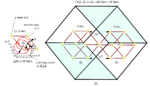
(a)                                                                      (b)

Figure 1: Illustrates a geometric model of bit-pair projections over $\theta$ forming a side-by-side tesseract. (a) shows a projection from the $\theta$ plane with a growing revolution that forms a volume containing 8 bits; (b) shows two sub-cubes denoting a bit-set of at least 16 bits under compression within an 8-bit cube. The equation above the hypercube represents this compression. The two-input $\pm\pi$-communication denoting entangled bit-set states, is viable for superdense coding operators to store data into a single qubit [bennett], as our future quantum compression model.

Further associating both fuzzy results with binary, each as an independent state, in total builds four simultaneous bit-pairs (each subcube of 8 bits), thus giving

$$\Phi_{\vee}(x) =\left(\forall x=0\in\mathcal{A}\cup\tilde{\mathcal{A}}\left|V_{Q_{x}}\right.\right)\vee\left(\forall x=1\in\mathcal{A}\cup\tilde{\mathcal{A}}\left|V_{Q_{x}}\right.\right)$$

$$\left.=\{0,1\}\rightarrow\{[0,1]\}\rightarrow\{\ 00,01,10,11\}\right.\,$$ (3a)

This is pairwise logic for many possibly contained (compressed) values of fuzzy as well as binary, and in its default set covers 8 states. By using a fuzzy unit on each bit-pair, we abstract the pairwise version to binary, which is an inverse process, or

$$\Phi_{\wedge}(x) =\left(\forall x=0|\{0,1\}\wedge\forall x=1|\{0,1\}\in\left\{\mathcal{A}|\tilde{\mathcal{A}}\right\}\cap\tilde{\mathcal{A}}\left|V_{Q_{x}}\!\rightarrow S_{Q_{x}}\right.\right)$$

$$\left.=\{0,1\}\leftarrow\{[0,1]\}\leftarrow\{\ 00,01,10,11\}\,\right.$$ (3b)

The fuzzy-binary and function $\Phi_{\wedge}$ uses logical operators and-or, negate and closures e.g., transitive closure [jacas] to generate crisp logic. Combining Eqs. (3a) and (3b), further outputs a fuzzy-binary and-or $\Phi_{\wedge\!\vee}$ or Eq. (1), such that

$$\left\{\left(\Phi_{\vee}\rightarrow\Phi_{\wedge}\right)(x)\right\}\wedge\left\{\left(\Phi_{\vee}\leftarrow\Phi_{\wedge}\right)(x)\right\}=\Phi_{\wedge\!\vee}(x)\left|S_{Q_{x}}\leftrightarrow V_{Q_{x}}\leftrightarrow V_{Q_{y}}\right.\$$ (3c)

where $\Phi_{\wedge\!\vee}(x)$ usage in the hypercube model, appears valid in its compression ratio

$$\mathcal{C}_{r}(x) =\frac{\mathcal{C}(Q_{x}\cdot Q_{x^{\prime}})}{Q_{x}+Q_{x^{\prime}}}=\frac{Q_{y}}{\mathcal{C}^{\prime}(Q_{y})}=\Phi_{\wedge\!\vee}\sum\beta(x)\vdash|xx^{\prime}|\leftrightarrow|y|$$

$$=(16\,{\rm bits})\leftrightarrow(8\,{\rm bits})=(2\,{\rm B})\leftrightarrow(1\,{\rm B})$$

$$=2\!:\!\!1\ \text{compression.}$$ (3d)

Remark 5.4.

Fuzzy convergence between maximum and minimum of $x\in[0,1]$ implies to many-valued logic [gottwald], now in abstraction by $\wedge,\vee$ operators.

and

Remark 5.5.

In recognition of Eqs. (5.3)-(5.3), the $\mathfrak{R}$ relationships in Eq. (1), denote an encoded-decoded, compressed-decompressed data projected into a hypercube, or conversely from its dual space of at least two subcubes on either end of the equation.

6 Compression Products Aimed by the FBAR Algorithm

To deliver a DE-transmission, our first approach was to study textual samples with binary constructs for a lossless compression, similar to the approach made by Shannon (1948) [shannon48] on English alphabet. Of course, with a main difference. We used standard characters in ASCII, with their 256 bit-byte combinations ($2^{8}$ bits, Lemma 2.1) on both binary and text. The resultant logic could be employed in the order of integer multiplications. For example, the RGB colors satisfy a huge number of possible combinations i.e., a 3-table consisting $256_{\rm R}\times 256_{\rm G}\times 256_{\rm B}\approx 16.7$ million combinations. This integer in turn supports other data types or non-English spoken languages (Unicode tables). In this paper, however, the primary scope for the first version of FBAR is $256\times 256=65536$ combinations. Its future versions, hypothetically grow toward much greater numbers beyond a 3-table, i.e., a 4-table for a $\mathcal{C}_{r}$ = 8:1 or 87.5% compression as $65536^{4\>\text{tables}}$ = 16 exabytes (EB). The latter is convenient for managing very large databases $\geq$ 1 TB. Such hypotheses are discussed in our future work section, Section LABEL:sect8, and translation table in Section 4.

7 FBAR Synthesis

Let an algorithm synthesize any logic state known to quantify information. To quantify, we need operators that operate on logic states. Those operators would be:

1. [(1)]

2. Boolean logic: Boolean operators as and, or, and not or negate. Boole (1848) [boole]

3. Fuzzy logic: Fuzzy operators as fuzzy-and, fuzzy-or, and not or negate. Zadeh (1965) [zadeh65]

4. Fuzzy-binary and-or (FBAR) combinatorial logic: synthesize all two above as fuzzy-binary-and, fuzzy-binary-or, and not or negate. This gives a lossless

   1. [(i.)]

   2. dynamic FBAR encoding and compression,

   3. static FBAR encoding and compression,

   4. FBAR decoding and decompression. Alipour and Ali (2010) [alipour10]

In this paper, we focus on 3.ii and 3.iii methods used in the algorithm to achieve “universal predictability.” This could only happen if both methods are conducted in terms of FBAR pairwise logic: synthesize all three logics via and-or and negate operators on pairs of 0, near 0, 1, and near 1 states to minimally transmit 8 bits, or

1. [(1)]

2. * a possible combination of 8 bits or $\{00,01,10,11\}$ denoting 4 possible bit-flag combinations (1-bit operators) on the four bit pairs (1-character input)

   1. [(i.)]

   2. FBAR bit-flag operators z for zero, n for negate, i as impurity, and p as purity operators on each pair of bits (definitions are given in Section 9)

   3. Employing znip operators in code, their minimum dimensional intersection as $\{\textbf{z},\textbf{n},\textbf{i},\textbf{p}\}\times\{\textbf{z},\textbf{n},\textbf{i},\textbf{p}\}$ allows such “transmissions” occur.

   This in total gives 4 fuzzy-binary or fb bits (definitions are given in Section 9)

3. * Thus, a minimum of 8 bits is transmitted via 4 bits. Since we need to represent data through standard 8-bit characters, the 4fb bits is concatenated with another 4fb bits, thus a pair of characters or 16 bits input are transmitted via 8fb bits output. This is an FBAR compression product.

7.1 Expected Outcomes

From (2)*, DE entropies are emerged denoting 50% and higher fixed compressions, regardless of the number of inputs given to the algorithm. This is theorized before our FBAR technique in Section 3, such as znip bivector operators are introduced and benefited from their product elements and conjunctive normal form (CNF) conversions [cockle, jackson], thereby tested and employed within the algorithm in Section 4. Also, by referring to Hamming distance and binary coding [hamming, sloane], a preamble on prefix coding to encode and decode data by operators is formulated. Higher fixed compressions are hypothesized for a negative entropy growth, once the minimum degree of a DE-compression or 50% is proven in theory and in practice. In Section 4, we demonstrate these entropies by proving the minimum degree of our DE-technique relative to its 4D-model of I/O data. We then prove decompression by satisfying the decoding method employed for the compressed data. Decompression is done by referring to byte addresses in the compressed file denoting the original input in the last two DE possibilities, (1)* and (2)*. We evaluate all of the hypotheses in the FBAR technique to demonstrate the validity of our concept. The efficiencies of compression in Theorem 1.1, are further evaluated through complexity measures on the algorithm’s code with bitrate performance. This quantity is measured for LDC temporal and spatial operations during I/O data access and process between compression and decompression states.

Chapter 3 FBAR Compression Theory

In this section, we formulate the FBAR synthesis in form of theorems and proofs aligned with its foundation from Section 4. Then, a 4D compression-decompression model is constructed by using FBAR operators and conversion functions on I/O data, as an improvement to the universal model from Section 5. The model should exhibit DE predictable values. It also encloses the DE values in form of bits, from a compressed form, to its decodable or decompressed form, in a lossless manner.

8 Reversible FBAR Compression Theorem and Proof

A reversible FBAR compression theorem begins with an assumption:

Assumption 3.1

Suppose for every $x$ character input we have a righthand character $x^{\prime}$, outputting a sequence $\mathcal{s}=(xx^{\prime})$. We assume our machine compiler compiles data on 8-bit words. We also assume $x$ and $x^{\prime}$ are from the ASCII table with a range of 0-255 characters. Let also any sequence of words be quantified by a length function $\ell$. Thus, the length of $\mathcal{s}$ in bits is $\ell(\mathcal{s})=$16 bits or 2 bytes ASCII.

Using Assumption 3.1 for a logical consequence, we hence submit a bit manipulation theorem on the given sequence $\mathcal{s}$, in terms of

Theorem 8.1.

Let the machine store a 2-byte binary input $xx^{\prime}$, as information. Once we manipulate a pure byte sequence $\beta=$11111111 to obtain $xx^{\prime}$ by four single bit-flags, one $y$ character is produced denoting the $xx^{\prime}$ content, equal to 8 bits.

Theorem 8.1 is analogous to the notion of Hamming distance [hamming, murdocca]: “the minimum number of substitutions required to change one string to another.” However, our case has no relevance to Hamming error-correction characteristics, and concerns the number of fuzzy pairwise bit substitutions. From Assumption 3.1, the notion of storing any sequence $\mathcal{s}$ in Theorem 8.1 becomes valid in terms of an array quantifying the contents of $\mathcal{s}$, or by convention

Remark 8.2.

The machine stores data in form of an array $A$ on sequence $\mathcal{s}$. Either $x$ or $x^{\prime}$ from $\mathcal{s}$, is of ASCII type measured in bpc, or entropy rate $H$.

Hence, a bivector product $\mathbf{e}_{ij}$ on subfields by Lounesto (2001) [lounesto], via its dual scalar element $h$ from Definition 2.3, self-contains and quantifies input $xx^{\prime}$ in terms of

Definition 8.3.

The $y$ character is stored in one of the rows $r$ in array $A_{r\times 4}$, where $r$ satisfies a possible number of ASCII combinations for $xx^{\prime}$. For all $y$, an $x\times x^{\prime}$ combination produces $r=256\times 256=65536$ rows with a subspace scalar of $h^{2}\mathbf{e}^{2}_{ij}$.

The $r$ for $xx^{\prime}$ by Definition 8.3, further shows the following to be true, if and only if, an interactive proof on FBAR logic is presentable (Section 8.1). Hence

Proposition 8.4.

The $y$ in $A$, holds single bit-flags that occupy the four columns $i$, $j$, $k$ and $l$, as biquaternion products from Proposition 2.1, in the $r\times 4$ array, or

$$A_{r\times 4}=A_{r\times(i\ j\ k\ l)}\ ,\ \ (\stackrel{{\scriptstyle 1}}{{i}}\ \stackrel{{\scriptstyle 2}}{{j}}\ \stackrel{{\scriptstyle 3}}{{k}}\ \stackrel{{\scriptstyle 4}}{{l}}) =h^{2}\left(\begin{array}[]{cccc}\mathbf{e}_{1}&\mathbf{e}_{2}&\mathbf{e}_{3}&\mathbf{e}_{4}\\ \end{array}\right)^{2}$$ (4b)

$$=\left(\begin{array}[]{cccc}h^{2}\mathbf{e}_{12}^{2}&h^{2}\mathbf{e}_{34}^{2}\\ \end{array}\right)$$ (4d)

where the bit-flags field is displayed by

$$\therefore xx^{\prime}\longrightarrow y\in\{r\times(i\ j\ k\ l)\}=65536\times(1_{x}1_{x^{\prime}}\ 1_{x}1_{x^{\prime}}\ 1_{x}1_{x^{\prime}}\ 1_{x}1_{x^{\prime}})$$ (4e)

and dimensionally measured by length $$\ell$$ as

$$\therefore\ell\left(A_{r\times 4}\right)=65536\times(2\,{\rm bits}\ 2\,{\rm bits}\ 2\,{\rm bits}\ 2\,{\rm bits})$$ (4f)

holding input data $$xx^{\prime} y$$, by a in the same field, in terms of

$$\therefore\ell\left(A_{r\times 4}\right)=65536\ \times 8\ \mathrm{bits}=64\ {\rm kilobytes}$$ (4g)

where $y=8\ \mathrm{bits}\in A_{r\times 4}=64\,{\rm K}$, affirming that $A$ is static. If the bivector $\mathbf{e}_{12}^{2}=-1$ for a pre-occupying character $x$, then its dual scalar is $h^{2}=-1$, otherwise $h^{2}=1$ for the post-occupying character $x^{\prime}$ by $\mathbf{e}_{34}^{2}=1$. Both conditions determine the subspace property on each $xx^{\prime}$ input as a superposing pair under compression. Thus, the compression products are orthogonally projective, positive and non-commutative.

Proof 8.5.

Suppose a $\varphi$ symbol denotes bit-flags for all $\mathbf{e}_{1234}$ in the $r\times 4$ array. According to Assumption 3.1, for the number of ASCII combinations on $r$, a total of $4\times 4\times 4\times 4=256$ on $x$, and 256 on $x^{\prime}$, satisfies 65,536 unique flag combinations. Its unit vector $\hat{{\bm{v}}}_{\varphi}$ whose coordinates are in one of the $1\times 4$ array dimensions, has a length of 1 bit with a scalar occupation. Thus, the $y$ character is stored in the $xx^{\prime}$ intersection $\cap$, where $\varphi$ values meet. This gives $y$ a different content not equal to $\varphi$, but representing the exact location of $xx^{\prime}$ in the sequence as well as content when $\varphi$ flags are translated. We create a static translation table to decode these flags based on where the $y$ character is stored i.e. the address with a reference point, or

$$\underbrace{\bigg{(}\underbrace{\overbrace{(\overbrace{4}^{\left(\begin{array}[]{cccc}1_{x}&1_{x}&1_{x}&1_{x}\\ \end{array}\right)}\times\overbrace{4}^{\left(\begin{array}[]{cccc}1_{x^{\prime}}&1_{x^{\prime}}&1_{x^{\prime}}&1_{x^{\prime}}\\ \end{array}\right)}}^{8\,{\rm bits}})}_{1\mathrm{st}\,16\,\text{combinations}}\cap\underbrace{(\overbrace{4\times 4}^{8\,{\rm bits}})}_{2\mathrm{nd}\,16}\bigg{)}}_{y\,\text{address}\,\cdots}$$ (5c)

$$\underbrace{\cap\bigg{(}\underbrace{(\overbrace{4\times 4}^{8\,{\rm bits}})}_{3\mathrm{rd}\,16}\cap\underbrace{(\overbrace{4\times 4}^{8\,{\rm bits}})}_{4\mathrm{th}\,16}\bigg{)}}_{\cdots\,y\,\text{address}}=8\,\mathrm{bits}$$ (5d)

stored as character $$y xx^{\prime}$$ in one of the 65,536 rows (prefix addresses) representing one of the four-dimensional combinations. These combinations are either 1st, 2nd, 3rd or 4th 16 combinations of bit-flags, for . Equation (5d) validates Proposition 8.4 equations for specific address and flags configuration. Specifically,

$$\forall\varphi\in A_{i,j,k,l}|\,\hat{{\bm{v}}}_{\varphi}=(1,0,0,0)\vee(0,1,0,0)\vee(0,0,1,0)\vee(0,0,0,1)\ ,\$$ (5e)

such that

$$\forall y\in A_{1\times 4}\subset A_{r\times 4}\ |\ \varphi\cdot A_{y}=\lambda_{xx^{\prime}}+\varrho_{xx^{\prime}}=(i,j,k,l)_{xx^{\prime}}+(i,j,k,l)_{xx^{\prime}}$$ (5f)

So, the translation table is a precalculated (prefix) rows-by-columns file on bit-flags, giving a reference point for the stored character $y$. The reference is a specific bit-flag combination from the 65,536 possible rows, constituting the $y$ address. The bit-flags set $\varphi$, represents all 16 bits content of $xx^{\prime}$, by manipulating a pure binary sequence $\beta=$ 1111 1111 recursively. This is shown in Eqs. (14). The byte is manipulated to obtain the binary content of $xx^{\prime}$. From Eq. (5f), let this manipulation start with the left-most bit to the right-most bit, operating on the left-byte $\lambda$ and the right-byte $\varrho$ of sequence $\mathcal{s}$. This gives a $y$ product on the $xx^{\prime}$ input, and is expressed by the following compression function:

$$g\circ f:\mathcal{s}_{\mathrm{in}}\rightarrow A$$

$$xx^{\prime}\mapsto g(f(xx^{\prime}))=f(y,\varphi)\,,$$

$$f(y,\varphi)=y\times\varphi_{xx^{\prime}}=y(\varphi_{x}+\varphi_{x^{\prime}})=y_{\varphi_{x}}+y_{\varphi_{x^{\prime}}}=y_{\varphi_{xx^{\prime}}}$$ (6)

Let $f$ be a function composition that maps the contents of $\mathcal{s}$ to the contents of array $A$, holding the same $xx^{\prime}$ contents via bit-flags $\varphi$. The bit-flags are occupied in form of character $y$. A two-variable function $f(y,\varphi)$ expresses the $y$ character carrying flags in array $A$, or its respective field ${\bf F}_{y}$. Its length is specified by

$$\ell(y_{\varphi})=\varphi A_{y}= \!\left[\left(\begin{array}[]{cccc}1_{i}&1_{j}&1_{k}&1_{l}\\ \end{array}\right)_{x}\cdot\left(\begin{array}[]{cccc}1_{i}&1_{j}&1_{k}&1_{l}\\ \end{array}\right)_{x}\right]$$ (9)

$$+\left[\left(\begin{array}[]{cccc}1_{i}&1_{j}&1_{k}&1_{l}\\ \end{array}\right)_{x^{\prime}}\cdot\left(\begin{array}[]{cccc}1_{i}&1_{j}&1_{k}&1_{l}\\ \end{array}\right)_{x^{\prime}}\right]$$ (12)

$$= \,\boldsymbol{\mho}(x)+\boldsymbol{\mho}(x^{\prime})=\hat{{\bm{\mu}}}_{x}\|\mathbf{e}\|^{2}\left(2\,\hat{{\bm{\mu}}}_{\beta_{x}}+2\,\hat{{\bm{\mu}}}_{\beta_{x^{\prime}}}\right)$$

$$= \,4\,{\boldsymbol{\mho}}+4\,{\boldsymbol{\mho}}=8\,\mathrm{bits}$$ (13)

In Eq. (13), the dual $\boldsymbol{\mho}$ manipulation method is of bivector type $|\mathbf{e}_{ij}|$ or $|\mathbf{e}_{kl}|$ from the norm $\|\mathbf{e}\|^{2}$ in Eqs. (2b), and so its product $\mathbf{e}\cdot\mathbf{e}$, is of a data-decoding process. The method is derived to alter the partitioned bit-pair values from $\beta$ in ${\bf F}_{y}$ to obtain original data, as if its values are of Pythagorean identity [leff] such that $8\,\hat{{\bm{\mu}}}_{\beta}=\mathop{\sum}_{n=1}^{8}\mathcal{s}(\sin^{2}\theta+\cos^{2}\theta)_{n}=11111111\,$ stored as a byte, or

$$\begin{array}[]{c}\left\{4\,{\boldsymbol{\mho}}\,{\rm manipulations\ on\ }y=8\,\hat{{\bm{\mu}}}_{\beta}=11111111=\beta{\rm\ to\ obtain\ }x\ +\right.\\ \left.4\,{\boldsymbol{\mho}}\,{\rm manipulations\ on\ }y=8\,\hat{{\bm{\mu}}}_{\beta}=11111111=\beta{\rm\ to\ obtain\ }x^{\prime}\right\}=8\,\mho\ ,\end{array}$$ (14c)

$$\therefore\, \varphi\left(\overbrace{\underbrace{(11)}}_{1{\rm bit}_{i}\times 1{\rm bit}_{i}}^{\frac{1}{4}y=y_{i}}\overbrace{\underbrace{(11)}}_{1{\rm bit}_{j}\times 1{\rm bit}_{j}}^{\frac{1}{4}y=y_{j}}\overbrace{\underbrace{(11)}}_{1{\rm bit}_{k}\times 1{\rm bit}_{k}}^{\frac{1}{4}y=y_{k}}\overbrace{\underbrace{(11)}}_{1{\rm bit}_{l}\times 1{\rm bit}_{l}}^{\frac{1}{4}y=y_{l}}\right)_{xx^{\prime}}\!\!=y_{xx^{\prime}}$$

$$=8\ {\rm bits}\to\underbrace{xx^{\prime}}_{16{\rm bits}}$$ (14d)

Thus, to store more $y$ characters in the field of rows, $r\times 4$, we establish a finite field $\mathbf{F}_{y}$ with $n$ elements. Therefore, $\mathbf{F}_{y}=\{y_{1},y_{2},\ldots,y_{n}\}$, represents a compression of sumset $\sum\mathcal{s}=(x_{1}x^{\prime}_{1}+x_{2}x^{\prime}_{2}+\ldots+x_{m}x^{\prime}_{m})$, achieving

$$\ell\left(\mathbf{F}_{y}\right)=\ell\left(\sum\limits_{i=1}^{m}{x_{i}x^{\prime}_{i}}\right)_{\mathrm{in}}\!\!\!\!\stackrel{{\scriptstyle\sum\limits_{r=1}^{65536}A_{r\times 4}}}{{\longrightarrow}}\!\ell\left(\sum\limits_{i=1}^{n}{y_{i}}\right)_{\mathrm{out}}\!=\frac{1}{2}\sum\mathcal{s}$$ (15)

Equations (14) and (15), show a fixed degree of double-efficiency over $y$, generating a decodable 50% compression.

Proposition 8.6.

The addressability of any original data is self-embedded in a grid file with 65,536 addresses, Eqs. (4g). For each double-character $xx^{\prime}$ input, one specific address is occupied by a character $y$ output, Eqs. (14). Translating the occupied address via a table whose row content returns original content, is by translating bit-flag combinations on a pure byte $\beta=\,$11111111 obtaining $xx^{\prime}$ from Eqs. (13)-(14).

8.1 Interactive Proof

Proof 8.7.

Suppose by default, we establish an ASCII combination on an $xx^{\prime}$ input. The total number of combinations is 256 ASCII characters for $x$, and 256 ASCII characters for $x^{\prime}$. Thus, $f(y)=256\,x\times 256\,x^{\prime}=65536$ $xx^{\prime}$. This gives an intersection of the combinations in total 65,536 8-bit addresses (64 KB). We prove the intersections using logic and subspace topology on array $A$. The combinations are integrable in space where bits reside as stored and then manipulated. Let a compact Hausdorff space [scarborough] contain a pure byte sequence $\beta=$ 11111111 for manipulation to obtain $xx^{\prime}$. The manipulation as a filter is done at a target point where space is locally compact. This results in compacted bits by associating all possible fuzzy pairwise bit manipulations, using bitwise operators OR |, and AND & in code. Therefore, the manipulation ‘11111111’ for a 2-byte content $xx^{\prime}$ is ‘$\texttt{11111111}+\texttt{11111111}$’. The association of manipulation is via bit-flags giving left-byte intersected with right-byte. This association of two 8-bit sets gives an 8-bit output. Interactively, $\forall\ xx^{\prime}\mapsto\{y\}_{i,j,k,l\in\mathbb{R}^{4}}$ we prove:

$$xx^{\prime}\stackrel{{\scriptstyle\mathrm{store}}}{{\longrightarrow}}A_{y}=\frac{xx^{\prime}}{\|\mathbf{e}\|}=\frac{xx^{\prime}}{\sqrt{\mathbf{e}\cdot\mathbf{e}}}=\frac{xx^{\prime}}{\sqrt{4}}=\left(\frac{1}{\sqrt{2}}x_{i}\,\frac{1}{\sqrt{2}}x_{j}\,\frac{1}{\sqrt{2}}x^{\prime}_{k}\,\frac{1}{\sqrt{2}}x^{\prime}_{l}\right)$$ (16a)

$$\therefore\ xx^{\prime}\stackrel{{\scriptstyle\mathrm{store}}}{{\longrightarrow}}\framebox{\bf{P}}\stackrel{{\scriptstyle\mathrm{filter}}}{{\longrightarrow}}f(y,\varphi)=\sqrt{|e_{12}|^{2}+|e_{34}|^{2}}=\sqrt{\frac{1}{2}x^{2}+\frac{1}{2}x^{\prime 2}}=8\,{\rm bits}$$ (16b)

Using the law of associativity in logic, the manipulative bits for $$xx^{\prime}$$ appear as

$$\therefore\, \left(\{8\,\mathrm{bits}_{x}\}\in\underbrace{i\times j}_{2\,{\rm dimensions}}\ni\{8\,\mathrm{bits}_{x}\}\right)\cap$$

$$\left(\{8\,\mathrm{bits}_{x^{\prime}}\}\in\underbrace{k\times l}_{2\,{\rm dimensions}}\ni\{8\,\mathrm{bits}_{x^{\prime}}\}\right)=\boldsymbol{\mho}(\beta)$$

$$=8\ {\rm dual\ \mho\ manipulations}=8\,{\rm bits}=y\times\varphi_{xx^{\prime}}\in\mathbb{R}^{4}$$ (16c)

and the address of $$y xx^{\prime} \varphi \beta$$ for is found via 1-bit flags operating on , such that

$$\therefore\ell(\varphi_{xx^{\prime}}) =\left(\{\underbrace{4_{\varphi\forall x}}_{4\,{\rm flags}}\}\in i\times j\ni\{\underbrace{4_{\varphi\forall x}}_{4\,{\rm flags}}\}\right)\cap\left(\{\underbrace{4_{\varphi\forall x^{\prime}}}_{4\,{\rm flags}}\}\in k\times l\ni\{\underbrace{4_{\varphi\forall x^{\prime}}}_{4\,{\rm flags}}\}\right)$$

$$=4\,{\rm bits}$$ (16d)

where a storage field $${\bf F} \varphi$$ covering all bit-flags is quantified in terms of

$$\ell\left({\bf F}_{\varphi}\right)=\ell\left(\prod\limits_{e=1}^{4}4\left(\begin{array}[]{cccc}1_{i}&1_{j}&1_{k}&1_{l}\\ \end{array}\right)_{e}\right)=\prod\limits_{e=1}^{4}\left(4_{i}+4_{j}+4_{k}+4_{l}\right)_{e}$$

$$\ \ \ =16_{1}\times 16_{2}\times 16_{3}\times 16_{4}={16^{4}{\rm bits}}=64\,{\rm kilobytes}$$ (16e)

So, $i\times j\times k\times l$ represents a binary address as a four-dimensional flag or a byte in a spatial field $\mathbb{R}^{4}$ topology. Therefore, $xx^{\prime}$ is distributed in 4 dimensions $i,j,k$ and $l$ by storing 1 $y$ character in the corresponding row. Now for the “storage field,” suppose we create a grid file G as a portable file with an empty space of 65,536 $i\times j\times k\times l$ rows, satisfying all possible combinations. This grid in specification should cover the $y$ field or ${\bf F}_{y}$ as well as bit-flag combinations. The $y$ field has a limit to store 1 to $n$, of $y$ characters corresponding to more inputs of $\mathcal{s}$. Let this be a sumset $\sum\mathcal{s}$ from Eqs. (14). Thus, we specify these possible address combinations with a multi-sum on the available dimensions of 1-bit flags $\varphi$, covering field ${\bf F}_{y}$, or

$$A_{y}\cap A_{\varphi}={\bf F}_{y}\times{\bf F}_{\varphi}={\bf F}_{y}\otimes\sum\limits_{1\leqslant i,j,k,l\leqslant 16}\varphi_{xx^{\prime}}=\framebox{{G}}$$ (17)

This, specifically builds our grid file multiplied with the sequences input $\mathcal{s}$ transposed matrix, as follows

$$\framebox{{G}}= \,\{y_{1},y_{2},\ldots,y_{m}\}$$

$$\times\mathop{\left[\begin{array}[]{cccccccccccccc}1&2&3&\cdots&16&1&1&1&1&1&1&1&\cdots&16\\ 1&1&1&1&1&2&3&\cdots&16&1&1&1&\cdots&16\\ 1&1&1&1&1&1&1&1&1&2&3&\cdots&\cdots&16\\ 1&1&1&1&1&1&1&1&1&1&1&1&\cdots&16\\ \end{array}\right]}\nolimits_{\sum\mathcal{s}}^{\rm T}$$ (18e)

$$=\{8\,{\rm bits},8\,{\rm bits},\ldots,8\,{\rm bits}\}\times 65536_{ijkl}=\mathcal{s}_{\,\rm out}$$ (18f)

Evidently, the way $$y_{i}$$ is stored and configured, is later decodable for an LDD, where

$$\left\{\mathcal{s}_{\,{\rm out}}\in\left.\framebox{{\bf G}}\,\right|1\,y\leq s\leq\ell\left({\bf F}_{y}\right)\right\}\ ,\ \ell\left(\framebox{{\bf G}}\right)=\ \ell\left({\bf F}_{y}\right)+64\,{\rm kilobytes}$$ (18g)

Ergo, by default, we occupy a $$y xx^{\prime} x x^{\prime} \mathcal{s} \sum\mathcal{s}=x_{1}x^{\prime}_{1}+x_{2}x^{\prime}_{2}+x_{3}x^{\prime}_{3}+x_{4}x^{\prime}_{4}=\texttt{resolved}$$ = 8 bits for an = 16 bits, since Eqs. (18) intersected 8-bit flags for with 8-bit flags for in the range of available rows in the grid file. So, if we exemplify a string of characters “resolved,” the sequence becomes . Thus, the allocated bit-flags with respect to byte addresses display,

$$\sum\mathcal{s}=64\,\mathrm{bits}\stackrel{{\scriptstyle\mathrm{store}\ \mathrm{as}}}{{\longrightarrow}}\mathbf{F}_{y} =\{y_{1},y_{2},y_{3},y_{4}\}\!\subset\!A_{65536\times 4}$$

$$=32\,{\rm bits}\in\|r\|=\frac{[1,4]}{65536}\ {\rm rows}\ ,$$

$${\rm where}\ |\mathbf{F}_{y}|=4\ |y_{i}\in[1\times 1\times 1\times 1\ ,\ 16\times 16\times 16\times 16]$$ (18h)

In this case, the rows magnitude $\|r\|$ is up to $\sqrt{1^{2}+4^{2}}=\sqrt{17}=4.12$ out of 65,536 rows, since we have a cardinality of 4$y$’s occupying the array or storage field ${\bf F}_{y}$, with a specific address to decode 64 original bits. This gives a decodable 50% compression plus a static size of 64 kilobytes.

8.2 FBAR Compression-Decompression Theorems

Following the Compression Proof 8.7, we specify an FBAR logic on I/O bit manipulations, delivering an FBAR compression theorem as follows:

Theorem 8.8.

Let the machine store a 2-byte binary input, $xx^{\prime}$, as information. Once we manipulate a pure byte sequence ‘11111111’ to obtain $xx^{\prime}$ by bitwise and-or, negate [boole], and close it by fuzzy transitive closure [jacas], one $y$ character is produced denoting the $xx^{\prime}$ content, equal to 8 bits.

From Theorem 8.8, following Theorem 8.1 proof, we deduce an FBAR compression $\mathcal{C}$ corollary,

Corollary 8.9.

The four combined operations, pairwise and-or, negate and fuzzy transitive closure on sequence $\mathcal{s}$, give a 50% fixed compression.

From Theorem 8.8, we further deduce a complete FBAR compression $\mathcal{C}$ corollary

Corollary 8.10.

The FBAR four combinatorial operations on any sequence $\mathcal{s}$ from $\sum\mathcal{s}=(x_{1}x^{\prime}_{1}+x_{2}x^{\prime}_{2}+\ldots+x_{m}x^{\prime}_{m})$ give the same compression ratio 2:1, or 50%.

Complementing Theorem 8.8 with a decompression $\mathcal{C}^{\prime}$ theorem, we deduce a complete FBAR compression-decompression theorem or $\mathcal{CC}^{\prime}$

Theorem 8.11.

Let a 1-byte $y$ output holding bit-flags of $\varphi$, represent a 2-byte binary input. This gives a 50% fixed compression. During compression, byte addresses are stored in a static address as (4$\times$4$)\times($4$\times$4) single bit-flags, once accessed and decoded via a translation table on $y$ and $\varphi$, a lossless decompression is obtained.

and obtainable by

Proposition 8.12.

Sequence $\mathcal{s}$ is compressed into $y$ whilst reconstructable via bit-flags held by $y$, where $\ell(y)=\ell\left(\frac{xx^{\prime}}{2}\right)=\frac{\mathcal{s}}{2}$ or 50% fixed $\mathcal{C}$ on $xx^{\prime}$ inputs. Once inputs are equally compressed via bit-flags in different locations of $y$, any $\mathcal{s}_{\,\mathrm{in}}$ is losslessly reconstructed. The specific address is where $y$ is stored amongst the 65,536 rows.

9 4D Bit-Flag Model Construction

9.1 I/O Operators Construction

To satisfy the practical application of our proof for Theorem 8.8, we need to construct the algorithm components with relevant operators to conduct an LDC-DD.

Proof 9.13.

Let a grid file component G be constructed according to Eqs. (18), with a translation table TT. To construct these two components, we intersect the dimensions of bit-flags $\varphi$ with each other in the $1\times 4$ matrix, for each LDC I/O. We partition $\varphi$ according to Eqs. (13), (16c) and (16e) in $i,j,k,l$ dimensions of G, resulting four bivector operators. Let those operators be z, n, i, p, where their paired combinational form, zn and ip, constructs in total the four dimensions. The static range $[\mathbf{zzzz}\ ,\ \mathbf{pppp}]$ for $[1,65536]$ rows, stores only one dynamic character output $y$, per two-character input $xx^{\prime}$:

$$\begin{split}&\exists\,xx^{\prime}=16\,{\rm bits}\in i\times j\times k\times l\ni y=8\,{\rm bits}\ ,\\ &\mathrm{iff}\ h^{2}\mathbf{e}^{2}_{1234}=\mathbf{znip}\stackrel{{\scriptstyle\mathrm{operates\ on}}}{{\longrightarrow}}xx^{\prime}\ \mathrm{for\ compression}\,.\ \end{split}$$ (19a)

Notation $$\ni \in y i,j,k,l$$, here, follows the set membership notation , symmetrically, such that is identifiable in the bivector dimensions. Now, we adapt the grid file range on the rows from Eqs. (18) to bit-flag operators, giving

$$\mathbf{znip}\stackrel{{\scriptstyle\mathrm{operates\ on}}}{{\longrightarrow}}xx^{\prime}=y\ ,{\rm where}$$

$$\mathbf{znip}\in i\times j\times k\times l=[\mathbf{zzzz}\ ,\ \mathbf{pppp}]$$

$$=[1\times 1\times 1\times 1\ ,\ 16\times 16\times 16\times 16]=[1\ ,\ 65536]$$ (19b)

where ${\bf z}$ is a zero or neutral operator, ${\bf n}$ a negate operator, ${\bf i}$ an impurity operator, ${\bf p}$ a purity operator, operating on bits. Suppose by definition, we apply and-or logic ($\wedge\vee$) to the ${\bf z}$ operator on bit pairs, thus

Definition 9.14.

For all ${\bf z}$, ${\bf z}$ on a pair of bits in the $x$ or $x^{\prime}$ binary, returns the same bits when and-or applied, where this applies to all remaining pairwise combinations, or

$$\mathbf{z}(0\wedge\vee 0)=00,\ \mathbf{z}(1\wedge\vee 1)=11,\ \mathbf{z}(0\wedge\vee 1)=01,\ \mathbf{z}(1\wedge\vee 0)=10.$$ (20a)

Then negation holds good for all pairwise bit combinations

Definition 9.15.

For all ${\bf n}$, ${\bf n}$ on a pair of bits in the $x$ or $x^{\prime}$ binary, negates the bits when and-or applied, where this applies to all remaining pairwise combinations

$$\mathbf{n}(\neg(0\wedge\vee 0))=11,\ \mathbf{n}(\neg(1\wedge\vee 1))=00,\ \mathbf{n}(\neg(0\wedge\vee 1))=10,$$

$$\mathbf{n}(\neg(1\wedge\vee 0))=01.$$ (20b)

From the laws of Boolean algebra covering $\wedge$, $\vee$ and $\neg$ operators, the defined $\mathbf{z}$ and $\mathbf{n}$ operators in consequence hold good as axioms:

Axiom 1.

Operator $\mathbf{n}$ is antecedent to negate all pairwise bit combinations. The consequent output is always the opposite of the given input.

and

Axiom 2.

Operator $\mathbf{z}$ is antecedent to pass all pairwise bit combinations. The consequent output is always as same as the given input.

We can now make the definitions of Eqs. (9.17) and (9.19) quite explicit as follows:

Definition 9.16.

For all z, z on any pair of bits in the binary of $x$ or $x^{\prime}$, returns the same bits, where this applies to all remaining pairwise combinations.

and

Definition 9.17.

For all n, n on any pair of bits in the binary of $x$ or $x^{\prime}$, returns negated bits, where this applies to all remaining pairwise combinations.

Now, suppose by definition, we apply transitive closure $\stackrel{{\scriptstyle\curvearrowright}}{{\longrightarrow}}$, to the ${\bf i}$ operator on bit pairs, acting as “operates on” from Eqs. (19), such that

Definition 9.18.

For all i, bit pairs in the binary of $x$ or $x^{\prime}$ is either 01 or 10. i closes with 1 for 01, and 0 for 10, or

$$\mathbf{i}(01)=0\stackrel{{\scriptstyle\curvearrowright}}{{\longrightarrow}}1=1,\ \ \ \mathbf{i}(10)=1\stackrel{{\scriptstyle\curvearrowright}}{{\longrightarrow}}0=0.$$ (21a)

and if applied to the ${\bf p}$ operator, we then have

Definition 9.19.

For all p, bit pairs in the binary of $x$ or $x^{\prime}$ is either 00 or 11. p closes with 1 for 11, and 0 for 00, or

$$\mathbf{p}(11)=1\stackrel{{\scriptstyle\curvearrowright}}{{\longrightarrow}}1=1,\ \ \ \mathbf{p}(00)=0\stackrel{{\scriptstyle\curvearrowright}}{{\longrightarrow}}0=0.$$ (21b)

The bit-pair operators from Eqs. (21a) and (21b), generate conflicting binary products in terms of

Paradox 3.1

Operator $\mathbf{i}$ is coincident with operator $\mathbf{p}$ in bit-pair products that end with 1 or 0. The consequent output after closure is $\mathbf{i}(10)=\mathbf{p}(00)$, $\mathbf{i}(01)=\mathbf{p}(11)$.

which is in code, addressed by

Solution 9.20.

We first consider a pure sequence of bits, ‘11111111’. We manipulate the bit-pairs in the sequence with ip, then its result by zn combinations for original data $xx^{\prime}$. Example (9.33) shall prove this.

Combining the z and n axioms with the i and p solution, further delivers

ip as an impure or pure pairwise bits’ dimension providing 16 combinations:

$$\begin{split}&{\bf iiii\ iiip\ iipi\ ipii\ piii\ iipp\ ippi\ ppii\ pipi\ ipip\ piip\ ippp}\\ &{\bf pipp\ ppip\ pppi\ pppp}\end{split}$$ (22a)

zn as a zero or negate pairwise bits’ dimension providing 16 combinations:

$${\bf zzzz\ zzzn\ zznz\ znzz\ nzzz\ zznn\ znnz\ nnzz\ nznz\ znzn\ nzzn\ znnn}$$

$${\bf nnnz\ nznn\ nnzn\ nnnn}$$ (22b)

Now, we establish a static solution using Eq. (17) and the combinations above for an LDC operation

Solution 9.22.

We build a grid file G based on these available combinations. The combinations constitute the finite field addresses $\mathbf{F}_{y}\times\mathbf{F}_{\varphi}$ as our static solution. This field gives a static number of rows and addresses for each compressed character $y_{i}$.

and the dynamic solution continuing the previous LDC operation is,

Solution 9.23.

The G grows in file size as a dynamic field of compressed characters $y_{i}$ in length, when more than 1 character is stored beyond its static range. So, we store the $1\,y$ character by the program in one of the 65,536 rows representing original data (two characters) within the intersected columns of the dimensions.

and its dynamic solution for an LDD operation, respectively, would be

Solution 9.24.

We access G by program code, invoking a comparator subroutine in our code. A $\mathcal{C}^{\prime}$ is achieved by traversing the $i\times j\times k\times l$ dimensions as the grid’s Hamming distance $d$ for each data read between fields $\mathbf{F}_{y}$ and $\mathbf{F}_{xx^{\prime}}$ via $\mathbf{F}_{\varphi}$.

So the question remains that: where should we establish distance $d$ between the prefix encoding and decoding levels of our $\mathcal{C}$ and $\mathcal{C}^{\prime}$ operations?

To answer this question, we need to succeed in Solution 9.24. For this, we recall Eqs. (16e)-(18), and consider the Hamming distance $d$ definition by Symonds (2007) [symonds], thus measuring our $d$ as follows:

Definition 9.25.

Hamming distance $d$ is measured between $n$-compressed characters stored with a minimum dynamic space of 64 K = 65,536 static rows of G, or as of Eq. (18g), in $\mathbf{F}_{y}+\,64\,$K, and their decodable 2$n$-input characters in a maximum static space as translation rows and columns in terms of $\{\mathbf{F}_{xx^{\prime}},\mathbf{F}_{r},\mathbf{F}_{\varphi},\mathbf{F}_{y}\}=\framebox{\bf TT}$. Therefore, the compressed characters $y_{i}$ are decoded by flag vectors $\varphi$ as carried in their address of the finite field $\mathbf{F}_{y}\times\mathbf{F}_{\varphi}=\framebox{\bf G}$.

Thus

Definition 9.26.

The number of coefficients in which they may differ in $\mathbf{F}_{y}$ to return original characters, is equal to the number of bit-pair manipulations $\boldsymbol{\mho}(\varphi A_{y})$ elicited from Eqs. (14) using znip operators based on Eqs. (19)-(9.19).

The last two definitions deduce the following

Definition 9.27.

Distance $d$ conserves the finiteness of character I/Os via the code comparator, comparing characters between $\{\mathbf{F}_{xx^{\prime}},\mathbf{F}_{y}\}\subset\framebox{\bf TT}$ and $\{\mathbf{F}_{y}\}\subset\framebox{\bf G}$, and will not recover any randomness between two or more compressed characters located in $1$ or $>1$ rows of $\mathbf{F}_{y}$ in G.

In addition,

Definition 9.28.

$d$ is 0 if at least 2 compressed $y$’s are stored in the same row address of $\mathbf{F}_{y}$ in G, which represent 4 original redundant $x$’s decoded from TT,

and

Definition 9.29.

Distance $d$ is $>0$ if compressed characters are located in 2 up to $k$ = 65536 grid rows, representing some original characters redundant, otherwise, all as different in TT.

Upon Definitions 9.25-9.29, the following solution is emerged to satisfy a lossless $\mathcal{C}$-and-$\mathcal{C}^{\prime}$ scenario of at least two compressed $y$’s stored in the G file component:

Solution 9.30.

According to Eqs. (17) and (18), and by Definitions 9.14-LABEL:def4.19, to decompress data losslessly, the 4 bit-flag operators znip, operate on $2\ y$’s in the finite field $\mathbf{F}_{y}$ in G, manipulating the byte in form of bit-pairs, which return $2\ xx^{\prime}$’s as their original. The original 4-character string is located in a TT file with all distances prefixed for each pair of $xx^{\prime}$. This transforms the grid to a distance of 0 when original characters are returned at the $\mathcal{C}^{\prime}$ phase for each read row $r$. The code comparator compares the unique znip row-by-column address from the table with the stored character in one of the grid file rows, from end-of-file to the file’s header.

Hence, benefiting from the Hamming distance propositions followed by their proofs in Symonds (2007) [symonds], and Eqs. (13)-(15), the usage of znip operators gives a maximum distance $d$ between vectors $\varphi_{\{y_{1},y_{2}\}}$ and $\varphi_{{xx^{\prime}}_{1}{xx^{\prime}}_{2}}$, as $d(\varphi_{\{y_{1},y_{2}\}},\varphi_{{xx^{\prime}}_{1}{xx^{\prime}}_{2}})=16$ for the number of required bit-pair manipulations (prefix dual-coding $\mho$). Therefore, as a bonus result, we immediately deduce the following two corollaries:

Corollary 9.31.

For two compressed characters $y_{1}$ and $y_{2}$, giving $d$ with respect to time $t$, as Hamming rate $R_{\mathbbm{H}}=d/t$ to search for a string match, results in a distance $d(\{y_{1},y_{2}\},{xx^{\prime}}_{1}{xx^{\prime}}_{2})=0$ during decompression $\mathcal{C}^{\prime}$. Let this distance be $d^{\prime}$.

Corollary 9.31 for the compressed characters $y_{1}$ and $y_{2}$, further gives

Corollary 9.32.

Part 1: The $\varphi_{y_{1}y_{2}}$ and $\varphi_{{xx^{\prime}}_{1}{xx^{\prime}}_{2}}$ vectors in output do not differ in the number of coefficients when time $t$ allows $\boldsymbol{\mho}(\{y_{1},y_{2}\},$ ${xx^{\prime}}_{1}{xx^{\prime}}_{2})=16\stackrel{{\scriptstyle\varphi}}{{\longrightarrow}}0$ grid transformations, such that from Eqs. (17)-(18), we firstly establish the integral on distance $d$ at time $t$

$$\forall R_{\mathbbm{H}}\in\mathcal{C}|R_{\mathbbm{H}}\!=\!\int_{\Delta t}\frac{d}{t}\,{\rm d}\,t\!=\!\frac{\|r\|}{\mathbf{t}}\int_{\min\|r\|_{\bf\emph{\bf{G}}}}^{d\left(\emph{\bf{G}},\emph{\bf{TT}}\right)}\!\!d(\{y_{1},y_{2}\},{xx^{\prime}}_{1}{xx^{\prime}}_{2})\,{\rm d}\,d=\!\frac{\Delta d}{\Delta t}$$

$$\mathrm{where}\ \exists\ \{y_{1},y_{2}\}\in\mathbf{F}_{y}\,|\,\ell\left(\mathbf{F}_{y}\right)=2\mathrm{B}+64\mathrm{K}=\ell\left(\framebox{\emph{\bf{G}}}\right)\ ,\ \mathbf{t}=1{\rm s}\ ,\,\mathrm{and}$$

$$\exists\ \{{xx^{\prime}}_{1},{xx^{\prime}}_{2}\}\in\mathbf{F}_{xx^{\prime}}\,|\,\ell\left(\mathbf{F}_{xx^{\prime}}\right)=4\mathrm{B}+64\mathrm{K}=\ell\left(\mathbf{F}\in\,\framebox{\emph{\bf{TT}}}\right)\,.$$ (23a)

Given the occupied $\varphi_{\{y_{1},y_{2}\}}$ and $\varphi_{{xx^{\prime}}_{1}{xx^{\prime}}_{2}}$ values in components set $\{\bf{G},\bf{TT}\}$ from a maximum number of rows $r$, between 4 original characters in TT and 2 compressed $y$’s in G, as distance $d$ at time $t$, in virtue of Eq. (13) and Lemma 2.1, we deduce

$$\therefore\ R_{\mathbbm{H}}=\!\int_{\Delta t}\frac{d}{t}\,{\rm d}\,t=\!\iint_{\frac{y_{1}}{2^{(8+8)}}}^{\max d}\dot{d}\,{\rm d}\,R=\frac{\|r\|}{\mathbf{t}}\!\int_{\frac{1}{k}\approx\,0}^{r^{\prime}\times\boldsymbol{\mho}(\varphi A_{y})}\!\!\!{\rm d}\,\boldsymbol{\mho}\ ,$$

$${\rm where}\,\begin{cases}\,r^{\prime}\in[1,k]_{\emph{\bf{TT}}}\\ \,t\in[0,\mathbf{t}]\end{cases}\hskip 113.81102pt$$ (23b)

Thus, the maximum value of $r^{\prime}$ rows holding the translation of the 2 compressed characters to their 4 original characters, is 2 rows in TT, giving a Hamming rate

$$\therefore R_{\mathbbm{H}}=\frac{2.23_{\bf G}}{k_{\bf TT}}\int_{\approx\,0}^{2_{\bf TT}(4+4)}\frac{r\times\boldsymbol{\mho}}{t}\,{\rm d}\,t=\frac{\Delta d}{\Delta t}\geq 0.0039\ {\rm Bps}\ ,$$ (23c)

whereby Definition 9.29, constant $k$ is 65,536 grid rows. Rate $R_{\mathbbm{H}}$ measured in Bps, is equal to the change of number of $\boldsymbol{\mho}$ bit-pair manipulations on the compressed data in an array of $r$ rows, relative to their original characters’ rows $r^{\prime}$, at time $t$.

Part 2: After applying znip operators in the Eq. (23c) upper integral limit, denoting a future $\mathcal{C}^{\prime}$ as stored addresses by $y$, we then compute its future rate returning $xx^{\prime}$

$$\ \exists\mathcal{C}^{\prime}\ni R^{\prime}_{\mathbbm{H}}=\frac{\|r^{\prime}\|}{\mathbf{t}}\int_{\max r^{\prime}_{\bf\emph{\bf{TT}}}}^{\|r\|_{\emph{\bf{G}}}}\!\!\!{\rm d}\,\boldsymbol{\mho} =\frac{\sqrt{\sum_{i=1}^{k}i^{2}}_{\bf G}}{\sqrt{k^{2}}_{\bf TT}}\int_{2}^{\frac{2.23}{k}}\frac{\boldsymbol{\mho}\times r^{\prime}}{t}\,{\rm d}\,t$$

$$=\frac{\Delta d}{\Delta t}\geq 295.6\,{\rm Bps}$$ (23d)

Thus, the total Hamming rate performing $\mathcal{C}$ and $\mathcal{C}^{\prime}$ is $\sum R_{\mathbbm{H}}=R^{\prime}_{\mathbbm{H}}+R_{\mathbbm{H}}\in\mathcal{CC}^{\prime}$. To evaluate Eq. (23d), we measure the total distance $d$ between $\mathcal{C}$ and $\mathcal{C}^{\prime}$ points via znip as their $\boldsymbol{\mho}$ string-match relation. Employing the Pythagoras’ theorem gives an imaginary part $\imath=\sqrt{-1}$ for $\mathcal{C}^{\prime}$, added to its conversed real part from $\mathcal{C}$ as follows

$$\begin{split}\sum d(\mathcal{C},\mathcal{C}^{\prime})&=\pm 2\pi\!\int_{\sqrt{\mathcal{C}}}^{\sqrt{\mathcal{C}^{\prime}}}\!\sqrt{\mathcal{C}}\>\>{\rm d}\,\mathcal{C}^{\prime}=2\pi\sqrt{\mathcal{C}^{2}-\mathcal{CC}^{\prime}}=|8.88|\,\mho\ ;\\ &\vdash\forall\,\boldsymbol{\mho}\in\mathbbm{C}\ell_{4}\left(\mathbbm{R}^{2^{\|\mathbf{e}\|}}\right)\left|\|\mathbf{e}\|\sum d(\mathcal{C},\mathcal{C}^{\prime})\right.\\ &=\left(\mathcal{C}\left(\sum\mathcal{s}_{\,\rm in}\right)\right)\boldsymbol{\mho}\left(\mathcal{C}^{\prime}\left(\sum\mathcal{s}_{\,\rm out}\right)\right)=\|dd^{\prime}\|=\sqrt{4}\mathcal{C}(d)\\ &\ \ \ \,-\sqrt{4}\mathcal{C}^{\prime}(d)=2\mathcal{C}(d)\,+2\mathcal{C}(d^{\prime})=8.88\|\mathbf{e}\|\approx 17.7\,\mho\ ,\end{split}$$

therefore

$$\|dd^{\prime}\| \vdash\left(\mathcal{C}\left(x_{1}x^{\prime}_{1}x_{2}x^{\prime}_{2}\right)\stackrel{{\scriptstyle d}}{{\longrightarrow}}\{y_{1},y_{2}\}\right)\mathbf{znip}\left(\mathcal{C}^{\prime}\left(\{y_{1},y_{2}\}\right)\stackrel{{\scriptstyle d^{\prime}}}{{\longrightarrow}}\{xx^{\prime}_{1},xx^{\prime}_{2}\}\right)$$

$$=\boldsymbol{\mho}\ \mathbf{znip}\ r^{\prime}=\boldsymbol{\mho}(\{y_{1},y_{2}\},{xx^{\prime}}_{1}{xx^{\prime}}_{2})\stackrel{{\scriptstyle+}}{{\bigcap}}\boldsymbol{\mho}({xx^{\prime}}_{1},{xx^{\prime}}_{2})\ ,\ {\rm ideally}$$

$$=\boldsymbol{\mho}\left(xx^{\prime}_{1}+xx^{\prime}_{2}\right)=\boldsymbol{\mho}(x_{1}x^{\prime}_{1}x_{2}x^{\prime}_{2})=\boldsymbol{\mho}\left(\sum\mathcal{s}_{\,\rm{out}}\right)=16+\imath\imath_{1234}^{\|\mathbf{e}\|}$$

$$=17\,\mho\ ,$$

and for the latterly-deduced result, we finally complement

$$\therefore\forall d\,\exists d^{\prime}\in\Delta d\,|\,\{\Delta d=(17.7-17)<1\,\mho\}\Leftrightarrow\{d\,\boldsymbol{\mho}\,d^{\prime}=16\stackrel{{\scriptstyle\varphi}}{{\longrightarrow}}0\,\mho\}\ .$$ (23e)

Operator $\stackrel{{\scriptstyle+}}{{\bigcap}}$ denotes a combinatorial string catenation and intersection of $y_{i}$ and $xx^{\prime}_{i}$ elements, emitted into a (discrete) concrete sequence $\mathcal{s}$. Equations (23e), show that there is no znip manipulation $\boldsymbol{\mho}$ to be made on $r^{\prime}\in\framebox{{TT}}$ to obtain $xx^{\prime}$ during $\mathcal{C}^{\prime}$, except a $d\,\boldsymbol{\mho}\,d^{\prime}$ string-search, match and catenate relationship, thus giving $d^{\prime}=0\,\mho$.

Corollaries 9.31 and 9.32 are possible, if and only if, component TT is accessed, thereby char addresses compared by code and their data decoded. Such $\varphi$ vectors agree in all coordinates of the grid’s $i\times j\times k\times l$ dimensions standing for an address during FBAR I/O operations. To keep matters simple, here is an example on a single compressed character $y$, spatially returning 2-original characters $xx^{\prime}$

Example 9.33.

If $xx^{\prime}=$ 01000000 00100100 $=@\$$, then by default 11111111 for $y$ is decoded, only when $y$ occupies $i\times j\times k\times l$ dimensions with a unique combination of operators. This combination is ${\bf ippp}\times{\bf niin}($11111111$)=$ 01111111 00010100 for $i\times j$, and this output intersected with the combination ${\bf znnn}\times{\bf znzz}($01111111 00010100$)=$ 01000000 00100100 for $k\times l$. The $y$ is stored in one of the rows out of 65,536 possible z, n, i, p combinations, which now returns characters $@\$$ = $xx^{\prime}$ by code.

Therefore, we reconstruct the pair $xx^{\prime}$ as our output. The output content is now equal to its original.

Corollary 9.32 assumes continuity on the whole interval quantified as a spatial-temporal type. It further proves Corollary 9.31 via Eqs. (23d)-(23e), with an output sequence $\mathcal{s}_{\rm\,out}$ from Eqs. (15) and (18). The spatial intervals in Eqs. (23a)-(23c) are delimited by the rows magnitude $\|r\|$ employed from Eqs. (18) in G, and its translation type $\|r^{\prime}\|$ in TT, where $r$ builds the maximum distance $d$ as the upper limit of integration. The temporal interval is given by $t$, and as conditioned in Eq. (23a), goes with a maximum ideal time $\mathbf{t}=1$ s, i.e., processor(s) and memory being able to handle an occupied space $\geq 64$ K I/O cases. The fluxion $\dot{d}$ in Eq. (23b), covers both temporal and spatial conditions from Eq. (23a), and absorbs any covariance of a great time and distance change (rate $R$) into a small one, resulting their $\Delta$ forms in Eq. (23c). The double integral, in this case, is absorbed into one succeeding integral as the future rate of $\mathcal{C}^{\prime}$ in Eq. (23d) proportional to the rate given by $\mathcal{C}$. Either rate is measured in bytes per second (Bps). It conveys to the implementation of prefix code and processing for pre-fuzzy bit-pair manipulations, which involves comparing addresses and rows for each set of compressed characters. For example, the minimum 295.6 Bps in Eq. (23d), corresponds to a minimum ASCII table-read requirement as 2$\times$128 translatable characters or 256 Bps to decode compressed data in FBAR. Thus, an extra 39.6 Bps memory allocation is needed to conduct a full $\mathcal{C}^{\prime}$. The Hamming distance used in Solutions 9.24 and 9.30 relative to components G and TT, is now subject to model construction for an I/O FBAR operation.

9.2 Algorithm Components and Model Construction

Using the string sample “resolved” from Eq. (18h), and considering the znip operators used in Example 9.33, suppose we establish a translation table TT like Table 2 to read $i\times j\times k\times l$ addresses (rows) containing 4 $y$’s (32 bits) from G. The TT file is fixed in size = 65,536 rows, and at least requires two key columns to translate $i\times j\times k\times l$, 1 $y$ binary content to $xx^{\prime}$ binary content and vice-versa.

At the $\mathcal{C}$ phase, the program writes G with ceratin characters, known as occupant chars as output $y$ in a specific row number. This number must correspond to an address that returns original characters when the occupant char is decompressed.

At the $\mathcal{C}^{\prime}$ phase, the program reads the grid file contents. From the occupant chars and the row address columns in TT or Table 2, the program returns original chars according to the ‘original char’ column. Occupant chars are those characters residing in the G file. Once the program identifies the occupant char in a particular row number, outputs $xx^{\prime}$ for that character according to the original char column from the TT file. This file in size is always 8 MB for any reference point as a bit-flag for an occupant char corresponding to the original file. The matrix vectors and I/O process layout for the example looks like this

$$\begin{array}[]{*{20}cc}&\\ \{\overbrace{\texttt{resolved}}^{\text{original text}}\}\stackrel{{\scriptstyle\text{read}}}{{\longrightarrow}}&\framebox{{P}}\\ &\updownarrow\\ &\framebox{{TT}}\\ \end{array}\stackrel{{\scriptstyle\text{write}}}{{\longrightarrow}}\framebox{\bf G}=\{\texttt{a},\texttt{b},\texttt{c},\texttt{d}\}\in\left\langle\mathbbm{R}^{4},\varphi\right\rangle$$ (24)

and the decomposition of the G component after being constructed and written by program P, is

$$\left[\begin{array}[]{c}\texttt{a}\\ \texttt{b}\\ \texttt{c}\\ \texttt{d}\\ \end{array}\right]\!\otimes\left\langle\overbrace{\left(\begin{smallmatrix}{\bf zizp}\\ {\bf zizp}\\ {\bf zini}\\ {\bf zini}\end{smallmatrix}\right)\!\times\!\left(\begin{smallmatrix}\bf npni\\ {\bf npzp}\\ {\bf zpzp}\\ {\bf zizi}\end{smallmatrix}\right)\!\times\!\left(\begin{smallmatrix}\bf zini\\ {\bf zini}\\ {\bf zizp}\\ {\bf zini}\end{smallmatrix}\right)\!\times\!\left(\begin{smallmatrix}\bf zizi\\ {\bf zpnp}\\ {\bf zini}\\ {\bf zinp}\end{smallmatrix}\right)}^{\left\langle\mathbbm{R}^{4},\varphi\right\rangle(\beta)}\right\rangle=\left[\begin{array}[]{ccc}\emptyset&\cdots&\emptyset\\ \vdots&\ddots\\ \texttt{d}&&\emptyset\\ \emptyset&\cdots&\emptyset\\ \vdots&\ddots\\ \texttt{c}&&\emptyset\\ \emptyset&\cdots&\emptyset\\ \vdots&\ddots\\ \texttt{a}&&\emptyset\\ \emptyset&\cdots&\emptyset\\ \vdots&\ddots\\ \texttt{b}&&\emptyset\\ \end{array}\right]_{\ell}$$ (41)

$$\text{where}\ \ell=64\texttt{K}+4\texttt{B}\ ,$$ (42)

and is a measured output denoting original data, such that

$$\begin{array}[]{*{20}cc}&\\ &\\ \{\texttt{re},\texttt{so},\texttt{lv},\texttt{ed}\}\!\longleftarrow\!\!\!&\!\!\!\!\!\!\framebox{{P}}\\ &\!\!\!\!\!\!\updownarrow\\ &\!\!\!\!\!\!\framebox{{TT}}\\ \end{array}\!\!\!\!\!\!\stackrel{{\scriptstyle\beta}}{{\longleftarrow}}\left\langle\overbrace{\left(\begin{smallmatrix}7\\ 12\\ 6\\ 1\end{smallmatrix}\right),\left(\begin{smallmatrix}11\\ 14\\ 6\\ 13\end{smallmatrix}\right),\left(\begin{smallmatrix}1\\ 6\\ 4\\ 2\end{smallmatrix}\right),\left(\begin{smallmatrix}13\\ 13\\ 15\\ 7\end{smallmatrix}\right)}^{\rm address}\right\rangle\!=\left\langle\texttt{a},\texttt{b},\texttt{c},\texttt{d}\right\rangle$$ (43)

In Eq. (42), the constructed G by empty values $\emptyset$ with 65,536 rows (64 K), has now an extra 4 bytes (chars) written to it by P. Program P before writing to G, accesses TT to write the 4 chars in specific locations denoting original data, given by (24) and (42). Later, for a decompression, the 4D function $\varphi$ in the P code, manipulates $\beta$ to obtain original data (its binary). This manipulation occurs when P refers to TT. The addresses of these 4 chars are identified in the TT file by P to reconstruct original data according to (43).

The left half of the input string ‘resolved’ in Eq. (24), is illustrated by a hypercube in Fig. 2. The grid file is constructed according to Eqs. (18), as well as TT for the code to access bit flags. Program P accesses the occupant chars a, b, c and d (known as $y$ in G) to return the original chars at the $\mathcal{C}^{\prime}$ phase. This phase is recognizable between components TT and P relationship ‘$\updownarrow$’ in Eqs. (24)-(43).

Table 2: The FBAR Translation Table

Row #	Bit-flag address	95 ASCII characters as “occupant chars”	Original char
		representing the “original char” column via
		the “bit-flag address” column
100	1x1x1x1	abcde…zABCDE …Z123…0’$\sim$!@$…$>,<$	${}^{\text{aa}}\hphantom{00}$
200	1x2x1x1	abcde…zABCDE …Z123…0’$\sim$!@$…$>,<$	¥${}^{\text{a}}\hphantom{00}$
300	1x3x1x1	abcde…zABCDE …Z123…0’$\sim$!@$…$>,<$	${\bullet}^{\text{a}}\hphantom{00}$
400	1x4x1x1	abcde…zABCDE …Z123…0’$\sim$!@$…$>,<$	${\copyright}^{\text{a}}\hphantom{00}$
⋮00	⋮00	⋮00	⋮00
65534 00	16x16x16x14	abcde…zABCDE …Z123…0’$\sim$!@$…$>,<$	ÿó00
65535 00	16x16x16x15	abcde…zABCDE …Z123…0’$\sim$!@$…$>,<$	ÿü00
65536 00	16x16x16x16	abcde…zABCDE …Z123…0’$\sim$!@$…$>,<$	ÿÿ00

aThe actual translation table contents or TT file for an LDC/LDD access and management bThe size of this component is approximately 8 MB.

Once the bit-flag addresses are identified by program P subroutines, thereby compared and interpreted in code, the original data is returned. This is done by bit manipulation $\boldsymbol{\mho}$ from Eqs. (14) on $\beta$ based on addresses to obtain original data (Example 9.33). The intersected addresses occupy in total 4 bytes for the 8-byte sample, since the number of stored chars in the G file is 4, or 4 bytes. Since an empty G is static in size, 64 K of rows, all the chars stored with addresses also denote a static allocation. The addresses in this sample respectively are 7x11x1x13, 12x14x6x13, 6x6x4x15 and 1x13x2x7. This is clearly specified in the four-dimensional vector space or storage subspace of bit-flags and addresses by Eq. (43). It is denoted by dimensional contents between the angle brackets $\langle\rangle$ notation. In this example, the occupant chars occupying the specific addresses are shown as $\langle\texttt{a},\texttt{b},\texttt{c},\texttt{d}\rangle$ in Eq. (43).

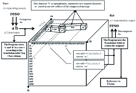
Figure 2: An I/O $\mathcal{CC}^{\prime}$ process on a ‘reso’ string is given in a 4D grid constructor. This constructor shows a 50% LDC with a DE state: the smaller inner-cubes in two places at the same time or “characters in $\pm\pi$-entanglement.” This model is a radix to higher DE-LDCs.

The motive for choosing this hypercube (Fig. 2) is anchored within the implementation of chars, being converted to binary as modeled back in Section 5, thereby generating self-contained flags within an input char of the G grid. This results in 50% pure compression, covering 2 chars per entry. From Axioms 1 and 2, and Definitions 9.16 to 9.28, emitting Eqs. (24)-(43), we put all of the emerging 1-bit znip flags into unique combinations to obtain double-efficiency. We intersect them with other znip’s representing a second char input. Therefore

Lemma 9.34.

Each character output is shared between $1\mathbf{ip}$ and $1\mathbf{zn}$ dimension, as a stored character. Containing $2\,{\rm chars}\leftrightarrow 2\mathbf{ip}+2\mathbf{zn}=4\,{\rm dimensions}$ is done in 65,536 rows or addresses. A minimally $2\,{\rm original\ chars}$ from $1\,{\rm stored\ char}$ is decoded.

The analogy of Lemma 9.34 is mappable to Moore’s Law and Knowledge Management by Gilheany [gilheany], stating: “each time a bit is added to the address bus width, the amount of memory that can be addressed is doubled.” Four-bit addresses allow the addressing of 16 bytes of memory, and in Lemma 9.34, are the 4 dimensions containing the 2 chars or $xx^{\prime}$. Eight bits allow the addressing of 256 bytes of memory, whereas 16 bits can address 65,536 bytes of memory (and extra work is necessary to address 640 kilobytes of memory, as was the case on the early IBM PCs). In the FBAR case, an 8-bit $y$ can address a 16-bit $xx^{\prime}$ in one of the 65,536 G file (portable memory) rows. Therefore, in terms of “an address information sent immediately following the control byte as a 16-bit word (65,536 possible addresses)” [smith], here, is compressed as a 16-bit $xx^{\prime}$ to an 8-bit $y$ character in G rows. So, $y$ in addition to a $\mathbf{znip}$ flag, plays the role of an 8-bit control byte for 65,536 possible addresses. Thus, we further deduce another lemma:

Lemma 9.35.

Lemma 9.34 gives a control double-byte $>$ a standard control byte for all intersecting addresses in G. Since an input data is doubly compressed as $\ell(xx^{\prime})=\ell(y)$, the static access of information in G is minimally, doubly faster than any other memory access when the compressed data is decoded.

The knowhow of these hypercube processes i.e., data access, compare, interpret after storage, is summarized in Table 3, and implemented in our practical section, Section 4, with performance results on the expected Hypothesis LABEL:hypo5.2 in Section LABEL:sect7.

9.3 Summary of Model and Theory

The 4D bit-flag model (hypercube) contains data for I/O transmissions. It maps contents in binary by intersecting their values in four dimensions using FBAR operators, suitable for any data type. The logic incorporated in this model, is of a combinatorial type, i.e. fuzzy, binary AND/OR logic. The rationale to the construction of this hypercube was to observe input characters, each pair of characters to be in two places at the same time. For imagery data types, an integer value is assigned instead, to satisfy an address representing two colors in two places simultaneously, out of the RGB color model for a 50% LDC (recall Section 6). Therefore, constructing $2^{n}$ memory addresses, in form of a grid file, gives a novel solution of how to compress data in doubles and pairs, losslessly. The fuzzy component of this logic is the middle point connecting binary with more possible states of logic. This connection of minimum to maximum number of states is defined in terms of an interrelated equation for all states of logic, and universal in all codeword representations. This was earlier introduced in Section 5. By combining Eqs. (24)-(43) layout on the sample, we deduce the following components’ paradigm. We later use this paradigm for the practical application of the algorithm to execute the operations held by components TT, P, G and original file O as follows:

$$\begin{array}[]{*{20}ccc}\mathrm{Decompression}&\\ &\\ \!\!\!\!\!\!\framebox{{O}}&\\ \!\!\!\!\!\!\uparrow&\\ \!\!\!\{\texttt{resolved}\}\stackrel{{\scriptstyle\mathrm{out}}}{{\longleftarrow}}\framebox{{P}}\stackrel{{\scriptstyle\mathrm{in}}}{{\longleftarrow}}\framebox{{G}}&\\ \ \ \ \ \ \ \ \ \ \ \updownarrow&&\\ \ \ \ \ \ \ \ \ \ \ \ \ \ \ \ \ \ \ \ \ \ \framebox{{TT}}\approx 8\,\mathrm{MB}&&\end{array}\!\!\!\!\!\!\!\!\!\left|\!\!\!\!\!\!\!\!\!\!\!\!\!\!\!\!\!\!\begin{array}[]{*{20}cc}&\mathrm{Compression}&\\ &\\ &\,\framebox{{O}}\longrightarrow\{\texttt{resolved}\}\!=\!8\>\mathrm{B}&\\ &\ \downarrow^{\mathrm{in}}&\\ &\ \ \ \ \ \ \ \ \ \ \ \framebox{{P}}\stackrel{{\scriptstyle\mathrm{out}}}{{\longrightarrow}}\framebox{{G}}\longrightarrow\{\texttt{a},\texttt{b},\texttt{c},\texttt{d}\}\!=\!4\,\mathrm{B}&\\ &\ \ \updownarrow&&\\ &\ \ \framebox{{TT}}\approx 8\,\mathrm{MB}&\end{array}\right.$$

Component O as original file, is where the original text or string is located. The practical process and structure of all LDC/LDD components are given in Section 4.

Chapter 4 FBAR Compression Practice

We implement the 4D model as the algorithm’s prototype based on the theoretical aspects of FBAR logic on I/O data transmissions. This prototype should perform DE predictable values. To do so, DE values are enclosed as bits of information, from a $\mathcal{C}$ form to its decoded $\mathcal{C}^{\prime}$ form in a lossless manner. Finally, we highlight certain details on the definiteness of future entropies supporting a growing negentropy, like Hyvärinen et al. [hyv], proving a universal predictability, contrasting the popular Shannon’s method of 1st order to 4th, inclusive of its general orders indeed.

10 FBAR Components, Process and Test

To fully implement an algorithm, one must understand how it works in terms of its testable structure and model representation. This is illustrated in Fig. 3. Furthermore, the algorithmic components must be introduced in terms of size, their process relationships, executables and data types. The $\mathcal{C}$ and $\mathcal{C}^{\prime}$ phases of the algorithm, iteratively use the following components: the G as the grid file, TT as the translation table file, and P as the program source code for I/O executions. The G file contains all compressed data representing the original characters. We call this the final compressed FBAR product or compressed file. We now introduce these components, their roles and functions for the $\mathcal{C}$ and $\mathcal{C}^{\prime}$ implementation as follows:

As proven in theory, from Eq. (42), the grid G component consists of 8-bit blank entries or $\emptyset$ in 65,536 rows, providing a possible ASCII (256$\times$256)= 64 K of static space for I/O data. The I/O data are processed by the P component. This component deals with original contents O component as original data which comprises of information built on one or more data types, given by the user. The O component, is our input sample and should be tested for a lossless compression $\mathcal{C}$, as well as decompression $\mathcal{C}^{\prime}$. The TT component consists of combinatorial details of any data as a table on bit-flags, row number and occupant chars, available to P.

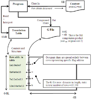
Figure 3: The 4D logic constructor files with an 8 B to 4 B compression.

The size of this table is static $\approx\,$8 MB for its self-contained information. Program P consists of lines of code to execute $\mathcal{C}\mathcal{C}^{\prime}$ procedures. It accesses O at the $\mathcal{C}$ phase, thereby constructs G and puts occupant chars in a specific bit-fag and row number (a prefix address) as compressed data, using TT information. At the $\mathcal{C}^{\prime}$ phase, the same program accesses G, and by reading both its contents and addresses identified by TT, reconstructs O. This has been illustrated in Section 9.3.

It is evident for each sample, at least one task $T$ is executed to perform compression parallel to decompression operations. Each conducted task allows one to evaluate the algorithm I/O’s in terms of temporal measurement, here bitrate, as well as spatial measurement as bpc or entropy. Once implementation is resolved on this small scale (1 O file input), test cases are maximized or extended to the large, in number, and in scale for I/O data integration. This scalability of I/O’s would guarantee the correctness of the code on FBAR logic requirements. For example, constructing an abstract release of a character reference column in the prefix TT component, based on standard keyboard characters, including whitespace “ ”, would not exceed 96 entries: 95 printable ASCII characters (decimal # 32-127) as shown in Table 2, plus 1 control character. The latter is used to create a block or a jump character, indicated as {/a, /b,…}, between every {1st, 2nd,…} 95-occupant char entry (or 95 $y$’s). At the $\mathcal{C}$ phase, this in total gives 95 $\times$ 2 = 190 original char entries per block, and is denoted by the ‘$\mathcal{C}$(char)’ column in Table 3. Note that, at the $\mathcal{C}^{\prime}$ phase, the program uses block chars to return {1st, 2nd, …, 95th} pair of the original chars, hence forming words and sentences in the right order.

Table 3: The FBAR I/O Character Process and Occupation Table

Row address	$\mathcal{C}$(char)#; $\mathcal{C}_{r}$	Original chars; total	Occupant char	Size (bits)
7x11x1x13	1   0 2:1=50%	0 re   0000 2	a	8 00
12x14x6x13	2   0 2:1=50%	0 so   0000 4	b	8 00
6x6x4x15	3   0 2:1=50%	0 lv   0000 6	c	8 00
1x13x2x7	4   0 2:1=50%	0 ed   0000 8	d	8 00
13x1x1x6	5   0 2:1=50%	0   f 0000 10	e	8 00
6x13x7x11	6   0 2:1=50%	0 or 0000 12	f	8 00
⋮   0	⋮    ⋮   000	0 ⋮ 0000 ⋮    0	⋮	⋮00
the same as last	96000   1:1=0%	$\mathbf{\infty}$    000 191	/a	16 00
8x12x8x12   0	97   0 2:1=50%	0 55   000 193	a	8 00
8x12x11x2   0	98   0 2:1=50%	0 5$   000 195	b	8 00
⋮   0	⋮    ⋮  0000	⋮ 0000 ⋮    0	⋮	⋮00

aThe TT file is used for each G file-read on the compressed chars as ‘occupant chars’ to return ‘original chars’ in the process. bThe table portrays the FBAR I/O products as original and compressed data per $\mathcal{CC}^{\prime}$ operation. The program compares values in the highlighted cells to return a $\mathcal{C}$ or $\mathcal{C}^{\prime}$ product.

The process design and development of the algorithm is illustrated in Fig. 3, with results listed in Table 3. The process begins with encoding input data using a dictionary coder, after which a high and low-state prefix fuzzy-binary conversions occur for compression. Recalling Eqs. (5.3)-(4g), each level of planar projection, from a lower 2D-layer to its upper, forms a 4D quaternions plane [arnold] or hypercube, as a 1-bit flag bi-vectors group [lounesto]. This group in the hypercube has its own augment in identifying impure 01, 10, and pure states of 11 and 00 for each converted data byte. In return, for an LDD, the converted binary data are recalled via a translation table (Table 2) as part of the dictionary or database represented by a set of occupying characters as the compressed version, denoting original data. We recall the original values from the TT file for each compressed occupying char, via a “grid file” as a portable memory grid or G on single bit-flags to decompress data. The FBAR dictionary consists of data references parsed into the translation table, building a static size of flag information, later used by the program for string value comparisons (the highlighted cells in Table 3).

11 Methods of Double-Efficiency

We implement the algorithm in form of a prototype. The prototype presents the FBAR model and its encoding/decoding components for DE compressions.

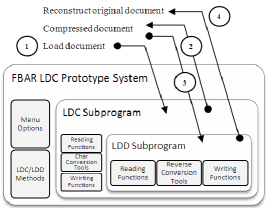
Figure 4: The structural components of the FBAR prototype.

As shown in Fig. 4, the prototype representing program P, compresses data by loading a document sample. The program uses a memory grid file G, which is a portable file containing single bit-flags in 65,536 rows or addresses. The translation of addresses for original characters, is given in a TT file rows with a static size of 8 MB, for any amount of input data manipulated by prefix code. The code interpreter decompresses data, once the flags are compared with the compression result. The decompression uses these prefix flags as compressed data, reconstructing the original document. All of these components, their processes and size are already proven in our theory, Section 9.2. In the following sections, we implement the algorithm components with results and evaluate its DE claim on I/O samples.

11.1 Algorithm Sample and Test

Assumption 3.1 holds good for the following algorithm:

Proposition 11.1.

From Assumption 3.1, suppose for every $x$ character input we have a righthand character $x^{\prime}$, its sequence appears as $\mathcal{s}_{\rm\,in}=xx^{\prime}$. For a long sequence $\mathcal{s}$, we suppose a sumset $\sum\mathcal{s}=(x_{1}x^{\prime}_{1}+x_{2}x^{\prime}_{2}+\ldots+x_{m}x^{\prime}_{m})$ to be our information input. Our objective in the program is to compress $\mathcal{s}$ to single-byte characters or $\mathbf{F}_{y}=\{y_{1},y_{2},\ldots,y_{n}\}$ or recall the Proof on Proposition 8.4.

Algorithm 4.1

Let program P get 2 Characters from left-to-right of sequence $\mathcal{s}$. If P continues in taking 2 more Characters with respect to time $t$, it instantiates a series of tasks $T_{1},T_{2},T_{3},\ldots,T_{n}$. These LDC tasks for each information processing cycle on the sequence appear as

$$\sum T\times\sum\mathcal{s}=(\underbrace{x_{1}x^{\prime}_{1}}_{T_{1}+}+\underbrace{x_{2}x^{\prime}_{2}}_{T_{2}+}+\ldots+\underbrace{x_{m}x^{\prime}_{m}}_{+T_{n}})\stackrel{{\scriptstyle\mathrm{get}}}{{\longrightarrow}}\framebox{\bf{P}}\stackrel{{\scriptstyle\mathrm{store}}}{{\longrightarrow}}\framebox{\bf{G}}\stackrel{{\scriptstyle\mathrm{out}}}{{\longrightarrow}}\mathbf{F}_{y}$$

$$\text{such that, }\mathbf{F}_{y}=\{y_{1},y_{2},\ldots,y_{n}\}\ .$$

The processing cycles in our algorithm should follow

1. [(1)]

2. Input: entering data into the program

3. Processing: performing operations on the data according to the TT file

4. Output: presenting the conversion results, in this case, the G file

5. Storage: saving data, or output for future use, in this case, the G file.

Now by applying the znip operators (as 1-bit flags) on Binary Sequence Character $\beta($‘1’$)=\texttt{11111111}$ as our default value in program P, to obtain the actual binary on each $xx^{\prime}$ per task $T$, we then code our algorithm:

Algorithm 1 comprises of LDC tasks, storing results in the G file. From the user, the program gets 2 chars, and inputs it from left-to-right of the file. The program by default contains a character ‘1’ assigning the two concatenated input chars to the ‘1’ (the customized $\beta$). Now, the program in line # 6 generates a character representing the 2 chars in the correct row (corresponding row) according to ASCII standard for the same characters. This is further instructed in line # 7 of the code, where the occupying row also represents an address of the compressed chars in the G file. The static translation table TT file is then used containing prefix addresses for every row out of 65,536 rows to translate, replacing one char with its original two chars for a 50% compression. This is expressed in line # 8, which gets the original 2 chars from TT per compressed char in G at the $\mathcal{C}^{\prime}$ phase of the algorithm. The remaining lines of the algorithm just denote the opposite condition where the new string is again requested from the user to input from the start.

AlgoLine0.1

Input: A set of LDC tasks and data conversions

Output: Storing LDC output to G file as a compressed string $y$

begin while There are still input characters in $\mathcal{s}$ do foreach 2 Characters from left-to-right of $\mathcal{s}$ do Get 2 input characters $x_{i}x_{i}^{\prime}$ ; AlgoLine0.2

Pack 1-bit flags on Binary Sequence Character ‘1’ = $x_{i}x_{i}^{\prime}$ ;AlgoLine0.3

Generate an occupant character $y_{i}$ according to the order of $x_{i}x_{i}^{\prime}$ ;AlgoLine0.4

Store 1 Occupant Character $y_{i}$ in the 1-bit flags row # in G file;AlgoLine0.5

AlgoLine0.6

if $y_{i}$ and row # is in the Translation Table then Continue getting the next 2 characters from left-to-right of $\mathcal{s}$ ; AlgoLine0.7

else Output the code for Pack as New String ; AlgoLine0.8

Restart Packing as New String in G file ;AlgoLine0.9

New String = $y$ ;AlgoLine0.10

endAlgoLine0.11

Algorithm 1 A lossless data compression sample

11

11

11

11

11

11

11

11

11

11

11

So, we can now initiate the $\mathcal{C}^{\prime}$ phase of the algorithm in terms of Algorithm 2. This algorithm comprises of LDD tasks, reconstructing results in a new file after reading from the G file relative to the TT file. From the G file, the program reads 1 character from right-to-left and reads the row number in line # 4, comparing it with the 65,536 available translations in the TT file (dictionary) in line # 5. The program reconstructs a string of translated characters and adds up newcomer characters to its string to build a full word, or a sentence of the original information, in line # 6-12, where # 12 denotes that, Old Code = New Code. Then the program cleans up the memory at line # 13.

Input: A set of LDD tasks and data conversions

Output: Decompressing G file as an LDD output $xx^{\prime}$

begin while Reading characters row-by-row from end-of-file G do foreach 1 character from right-to-left of string $y$ do Read row # ; AlgoLine0.1

AlgoLine0.2

if Character $y_{i}$ is not in (row # and Occupant Character) columns of TT file then New String $z$ = Get translation of Old Code ; AlgoLine0.3

New String $z$ = String $z$ + Character ;AlgoLine0.4

else Get translation of Old Code ; AlgoLine0.5

Character $z_{i}$ = 1st or 2nd or …or nth 2 characters in String ;AlgoLine0.6

Replace Character with 2 new characters from the TT file ;AlgoLine0.7

New String $z$ = $xx^{\prime}$ ;AlgoLine0.8

Delete temporary row # and row characters ;AlgoLine0.9

endAlgoLine0.10

Algorithm 2 A lossless data decompression sample

10

10

10

10

10

10

10

10

10

10

Relevant to the example provided in Algorithm 2, we further particularize an LDD in Algorithm 3, which is equivalent to Algorithm 2.

Algorithm 3 comprises of LDD tasks sampled from Algorithm 2, practicing a 16-byte (2-char) concatenation of the compressed chars $y_{i}=$ d then c then b then a (in lines # 8, 10, 12, 14), reconstructing a 64-byte result after the concatenation operation is done. This reconstruction of original chars occurs in a new file after reading from the G file relative to the TT file.

From the G file, the program reads 1 char from right-to-left pre-positioned to a block char and reads the row number in line # 4-6, comparing it with the 65,536 available translations in the TT file, in line # 7. Finally, The program reconstructs a string of translated characters from line # 8 up to line # 14, and adds up (concatenate) newcomer characters to its string to reconstruct the full word as the output given in line # 15, in this case ‘resolved’.

Input: A set of LDD tasks and data conversions

Output: Decompressing G file as an LDD output ‘resolved’

begin while Reading characters row-by-row from end-of-file G do foreach Last Block Character $y_{i}$ do if Character $y_{i}$ is a Block Character then Read Character pre-positioned to Block Character ; AlgoLine0.1

Read row # ;AlgoLine0.2

Get row address from TT file ;AlgoLine0.3

if Character $y_{i}$ =‘d’ and row address = ‘1x13x2x7’ then Output String =‘ed’ ; AlgoLine0.4

else if Character $y_{i}$ =‘c’ and row address = ‘6x6x4x15’ then Output String =‘lv’+‘ed’ = ‘lved’ ; AlgoLine0.5

else if Character $y_{i}$ =‘b’ and row address = ‘12x14x6x13’ then Output String =‘so’+‘lved’ = ‘solved’ ; AlgoLine0.6

else if Character $y_{i}$ =‘a’ and row address = ‘7x11x1x13’ then Output String =‘re’+‘solved’ = ‘resolved’ ; AlgoLine0.7

else Print no data or null compressed ; AlgoLine0.8