Simplification paths in the Pachner graphs
of closed orientable 3-manifold triangulations

Abstract

It is important to have effective methods for simplifying 3-manifold triangulations without losing any topological information. In theory this is difficult: we might need to make a triangulation super-exponentially more complex before we can make it smaller than its original size. Here we present experimental work that suggests the reality is far different: for an exhaustive census of 81 800 394 one-vertex triangulations that span 1 901 distinct closed orientable 3-manifolds, we never need to add more than two extra tetrahedra, we never need more than a handful of Pachner moves (or bistellar flips), and the average number of Pachner moves decreases as the number of tetrahedra grows. If they generalise, these extremely surprising results would have significant implications for decision algorithms and the study of triangulations in 3-manifold topology.

Key techniques include polynomial-time computable signatures that identify triangulations up to isomorphism, the isomorph-free generation of non-minimal triangulations, theoretical operations to reduce sequences of Pachner moves, and parallel algorithms for studying finite level sets in the infinite Pachner graph.

ACM classification F.2.2; G.2.1; G.2.2; D.1.3.

Keywords Triangulations, 3-manifolds, Pachner moves, isomorphism signatures, isomorph-free enumeration, 3-sphere recognition

Journal version

This is the journal version of [9], which was presented at the 27th Annual Symposium on Computational Geometry. This journal version contains significant new material.

The study has been expanded from just 3-sphere triangulations to include all closed prime orientable 3-manifolds, it examines average-case as well as worst-case behaviour, and it also analyses moves that connect distinct minimal triangulations of the same 3-manifold. Section 4 contains several new algorithms, through which the loose upper bounds of [9] have been replaced with smaller bounds, many of which are now tight. The analysis of pathological cases in Section 5 and the detailed specification of isomorphism signatures in the appendix are both new. The final discussion in Section 6 is significantly richer, and raises new issues involving generic complexity.

1 Introduction

Triangulations of 3-manifolds are ubiquitous in computational knot theory and low-dimensional topology. They are easily obtained and offer a natural setting for many important algorithms.

Computational topologists typically allow triangulations in which the constituent tetrahedra may be “bent” or “twisted”, and where distinct edges or vertices of the same tetrahedron may even be joined together. Such triangulations (sometimes called generalised triangulations) can describe rich topological structures using remarkably few tetrahedra. For example, the 3-dimensional sphere can be built from just one tetrahedron, and more complex spaces such as non-trivial Seifert fibred spaces can be built from as few as two [25].

An important class of triangulations is the one-vertex triangulations, in which all vertices of all tetrahedra are identified together as a single point. These are simple to obtain [18, 24], and they are often easier to deal with both theoretically and computationally [6, 17, 24].

Keeping the number of tetrahedra small is crucial in computational topology, since many important algorithms are exponential (or even super-exponential) in the number of tetrahedra [5, 6]. To this end, topologists have developed a rich suite of local moves that allow us to change a triangulation without losing any topological information [2, 26]. The ultimate aim is to simplify the triangulation, i.e., reduce the number of tetrahedra, although the triangulation might (temporarily) need to become more complex along the way.

The most basic of these moves are the four Pachner moves (also known as bistellar moves). These include the 3-2 move (which reduces the number of tetrahedra but preserves the number of vertices), the 4-1 move (which reduces both numbers), and also their inverses, the 2-3 and 1-4 moves. It is known that any two triangulations of the same closed 3-manifold are related by a sequence of Pachner moves [34]. Moreover, if both are one-vertex triangulations then in most cases we can relate them using 2-3 and 3-2 moves alone [24].

However, little is known about how difficult it is to simplify a triangulation, or to convert one triangulation into another, using Pachner moves. In a series of papers, Mijatović develops upper bounds on the number of moves required for various classes of 3-manifolds [29, 30, 31, 32]. All of these bounds are super-exponential in the number of tetrahedra, and some even involve exponential towers of exponential functions. For simplifying one-vertex triangulations using only 2-3 and 3-2 moves, no explicit bounds are known at all.

Simplification is tightly linked to the important recognition problem, where we are given an input triangulation $\mathcal{T}$ and a target 3-manifold $\mathcal{M}$, and asked whether $\mathcal{T}$ triangulates $\mathcal{M}$. The recognition problem is decidable but extremely difficult. A general algorithm comes as a consequence of Perelman’s celebrated proof of the geometrisation conjecture [21], but due to its intricate and multi-faceted nature, the algorithm remains computationally intractable and no explicit bound on its running time is known.

Some special cases of the recognition problem are more approachable. A notable case is 3-sphere recognition (where $\mathcal{M}=S^{3}$): this plays an key role in other important topological algorithms such as connected sum decomposition [18, 20] and unknot recognition [15], and is also important for computational 4-manifold topology. The original 3-sphere recognition algorithm of Rubinstein [35] has been improved significantly over time [6, 7, 18, 36], and although it remains worst-case exponential, it is now highly effective in practice for moderate-sized problems [7].

We can use Pachner moves to solve recognition problems in two ways:

• For the classes of manifolds $\mathcal{M}$ studied by Mijatović [29, 30, 31, 32], and in particular the 3-sphere [29], Pachner moves give a direct recognition algorithm: select a well-known “canonical” triangulation $\mathcal{T}_{c}$ of $\mathcal{M}$, and try to convert the input triangulation $\mathcal{T}$ into $\mathcal{T}_{c}$ by testing every possible sequence of Pachner moves up to Mijatović’s upper bound. Return “true” if and only if a successful conversion was found.

• For all manifolds $\mathcal{M}$, Pachner moves also give a hybrid recognition algorithm: begin with a fast and/or greedy procedure to simplify $\mathcal{T}$ as far as possible within a limited number of moves. If we reach a well-known canonical triangulation of $\mathcal{M}$ then return “true”; otherwise run the full recognition algorithm (such as Rubinstein’s algorithm for the case $\mathcal{M}=S^{3}$) on our new, and hopefully simpler, triangulation.

Direct algorithms are, at present, completely infeasible: Mijatović’s bounds are super-exponential in the number of tetrahedra, and the running times are super-exponential in Mijatović’s bounds. Even for the trivial case of 3-sphere recognition with one tetrahedron, a direct algorithm must test all possible sequences of $\sim 2.4\times 10^{6027}$ Pachner moves.

The hybrid method, on the other hand, is found to be extremely effective in practice. Experience with 3-sphere recognition software [3] suggests that when $\mathcal{T}$ is indeed the 3-sphere, the greedy simplification almost always gives a canonical triangulation, which means that the slower Rubinstein method is almost never required.

In the context of Mijatović’s results, this effectiveness of the hybrid method is unexpected, and forms a key motivation for this paper. More broadly, the aims of this paper are:

1. to measure how difficult it is in practice to relate two triangulations of a 3-manifold using Pachner moves, or to simplify a 3-manifold triangulation to use fewer tetrahedra;

2. to understand why greedy simplification techniques work so well in practice, despite the prohibitive theoretical bounds of Mijatović;

3. to investigate the possibility that Pachner moves could be used as the basis for a direct 3-sphere recognition algorithm that runs in sub-exponential time.

We restrict our attention to closed prime orientable 3-manifolds, as well as the important case $\mathcal{M}=S^{3}$ (which is not prime). We also restrict our attention to one-vertex triangulations with 2-3 and 3-2 moves, which is the most relevant setting for computation.

Fundamentally this is an experimental paper, though the theoretical underpinnings are interesting in their own right. Based on an exhaustive census of almost 150 million triangulations, including 81 800 394 one-vertex triangulations of 1 901 distinct 3-manifolds, the answers to the questions above appear to be:

1. we can relate and simplify one-vertex triangulations using remarkably few Pachner moves, and the average number of moves decreases as the number of tetrahedra grows;

2. both procedures require us to add at most two extra tetrahedra, which explains why greedy simplification works so well;

3. the number of moves required in the worst case to simplify a 3-sphere triangulation grows extremely slowly, to the point where sub-exponential time 3-sphere recognition may indeed be possible.

These observations are extremely surprising, especially in light of Mijatović’s bounds. For arbitrary manifolds, observation (ii) does not generalise: in Section 5 we construct larger triangulations of graph manifolds, beyond the limits of our census, for which three extra tetrahedra are required. In the case of the 3-sphere, no such counterexamples are known. If (iii) can be proven in general—yielding a sub-exponential time 3-sphere recognition algorithm—this would be a significant breakthrough in computational topology.

In Section 2 we outline preliminary concepts and introduce Pachner graphs, which are infinite graphs whose nodes represent triangulations and whose arcs represent Pachner moves. These graphs are the framework on which we build the rest of the paper. We define simplification paths through these graphs, as well as the key quantities of length and excess height that we seek to measure.

We follow in Section 3 with two key tools for studying Pachner graphs: an isomorph-free census of all closed 3-manifold triangulations with $\leq 9$ tetrahedra (which gives us the nodes of the graphs), and isomorphism signatures of triangulations that can be computed in polynomial time (which allow us to construct the arcs of the graphs). Here we also prove that the census grows at a super-exponential rate, despite its strong topological constraints.

Section 4 introduces theoretical techniques for “reducing” paths through Pachner graphs, and describes parallel algorithms that bound both the length and excess height of such paths. These algorithms are designed to work within the severe time and memory constraints imposed by the super-exponential census growth rate. This section also presents the highly unexpected experimental results outlined above.

In Section 5 we study pathological cases, including the census triangulations that are most difficult to simplify, as well as the graph manifold constructions mentioned above. We finish in Section 6 by exploring the wider implications of our experimental results, in particular for the worst-case and generic complexity analysis of topological decision problems.

All code was written using the topological software package Regina [3, 10].

2 Triangulations and the Pachner graph

A 3-manifold triangulation of size $n$ is a collection of $n$ tetrahedra whose $4n$ faces are affinely identified (or “glued together”) in $2n$ pairs so that the resulting topological space is a closed 3-manifold. We are not interested in the shapes or sizes of tetrahedra (since these do not affect the topology), but merely the combinatorics of how the faces are glued together. Throughout this paper, all triangulations and 3-manifolds are assumed to be connected.

We do allow two faces of the same tetrahedron to be identified, and we also note that distinct edges or vertices of the same tetrahedron might become identified as a by-product of the face gluings. A set of tetrahedron vertices that are identified together is collectively referred to as a vertex of the triangulation; we define an edge or face of the triangulation in a similar fashion.

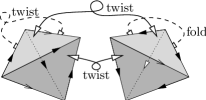
Figure 1: A 3-manifold triangulation of size $n=2$

Figure 1 illustrates a 3-manifold triangulation of size $n=2$. Here the back two faces of the first tetrahedron are identified with a twist, the front faces of the first tetrahedron are identified with the front faces of the second using more twists, and the back faces of the second tetrahedron are identified together by directly “folding” one onto the other. This is a one-vertex triangulation since all eight tetrahedron vertices become identified together. The triangulation has three distinct edges, indicated in the diagram by three distinct arrowheads.

For a given 3-manifold $\mathcal{M}$, a minimal triangulation of $\mathcal{M}$ is a triangulation of $\mathcal{M}$ that uses the fewest possible tetrahedra.

Not every pairwise gluing of tetrahedron faces results in a 3-manifold triangulation. Given $n$ tetrahedra whose faces are affinely identified in pairs, we obtain a 3-manifold triangulation if and only if: (i) every vertex of the triangulation has a small regular neighbourhood bounded by a sphere (not some higher-genus surface), and (ii) no edge of the triangulation is identified with itself in reverse.

The four Pachner moves describe local modifications to a triangulation. These include:

• the 2-3 move, where we replace two distinct tetrahedra joined along a common face with three distinct tetrahedra joined along a common edge;

• the 1-4 move, where we replace a single tetrahedron with four distinct tetrahedra meeting at a common internal vertex;

• the 3-2 and 4-1 moves, which are inverse to the 2-3 and 1-4 moves.

These four moves are illustrated in Figure 2. Essentially, the 1-4 and 4-1 moves retriangulate the interior of a pyramid, and the 2-3 and 3-2 moves retriangulate the interior of a bipyramid. It is clear that Pachner moves do not change the topology of the triangulation (i.e., the underlying 3-manifold remains the same). Another important observation is that the 2-3 and 3-2 moves do not change the number of vertices in the triangulation.

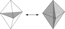
(a) The 2-3 and 3-2 moves

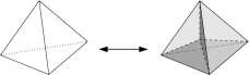
(b) The 1-4 and 4-1 moves

Figure 2: The four Pachner moves for a 3-manifold triangulation

Two triangulations are isomorphic if they are identical up to a relabelling of tetrahedra and a reordering of the four vertices of each tetrahedron (that is, isomorphic in the usual combinatorial sense). Up to isomorphism, there are finitely many distinct triangulations of any given size.

Pachner originally showed that any two triangulations of the same closed 3-manifold can be made isomorphic by performing a sequence of Pachner moves [34]. Matveev later strengthened this result to show that any two one-vertex triangulations of the same closed 3-manifold with at least two tetrahedra can be made isomorphic through a sequence of 2-3 and/or 3-2 moves [24]. The two-tetrahedron condition is required because it is impossible to perform a 2-3 or 3-2 move upon a one-tetrahedron triangulation (each move requires two or three distinct tetrahedra).

In this paper we introduce the Pachner graph, which describes how distinct triangulations of a closed 3-manifold can be related via Pachner moves. We define this graph in terms of nodes and arcs, to avoid confusion with the vertices and edges that appear in 3-manifold triangulations.

Definition (Pachner graph).

Let $M$ be any closed 3-manifold. The Pachner graph of $M$, denoted $\mathscr{P}(M)$, is an infinite graph constructed as follows. The nodes of $\mathscr{P}(M)$ correspond to isomorphism classes of triangulations of $M$. Two nodes of $\mathscr{P}(M)$ are joined by an arc if and only if there is some Pachner move that converts one class of triangulations into the other.

The restricted Pachner graph of $M$, denoted $\mathscr{P}_{1}(M)$, is the subgraph of $\mathscr{P}(M)$ defined by only those nodes corresponding to one-vertex triangulations. The nodes of $\mathscr{P}(M)$ and $\mathscr{P}_{1}(M)$ are partitioned into finite levels $1,2,3,\ldots$, where each level $n$ contains the nodes corresponding to $n$-tetrahedron triangulations.

Figure 3: Levels 1–3 of the restricted Pachner graph of the 3-sphere

It is clear that the arcs are well-defined (since Pachner moves are preserved under isomorphism), and that arcs do not need to be directed (since each 2-3 or 1-4 move has a corresponding inverse 3-2 or 4-1 move). In the full Pachner graph $\mathscr{P}(M)$, each arc runs from some level $i$ to a nearby level $i\pm 1$ or $i\pm 3$. In the restricted Pachner graph $\mathscr{P}_{1}(M)$, each arc must describe a 2-3 or 3-2 move, and must run from some level $i$ to an adjacent level $i\pm 1$. Figure 3 shows the first few levels of the restricted Pachner graph of the 3-sphere.

We can now reformulate the results of Pachner and Matveev as follows:

Theorem 2.1 (Pachner, Matveev).

The Pachner graph of any closed 3-manifold is connected. If we delete level 1, the restricted Pachner graph of any closed 3-manifold is also connected.

To simplify a triangulation we essentially follow a path through $\mathscr{P}(M)$ or $\mathscr{P}_{1}(M)$ from a higher level to a lower level, motivating the following definitions:

Definition (Simplification path).

A simplification path is a directed path through either $\mathscr{P}(M)$ or $\mathscr{P}_{1}(M)$ from a node at some level $i$ to a node at some lower level $<i$.

Definition (Length and excess height).

Let $p$ be any path through $\mathscr{P}(M)$ or $\mathscr{P}_{1}(M)$ from level $i$ to level $j$. The length of $p$ is the number of arcs it contains. The excess height of $p$ is the smallest $h\geq 0$ for which the entire path stays in or below level $(\max\{i,j\}+h)$.

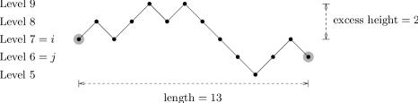
Figure 4: Measuring length and excess height

Figure 4 illustrates a path of length 13 and excess height 2. For simplification paths, the length and excess height measure how difficult it is to simplify a triangulation: the length measures the number of Pachner moves, and the excess height measures the number of extra tetrahedra required.

To simplify a 3-sphere triangulation, the only known bounds on length and excess height are due to Mijatović [29]:

Theorem 2.2 (Mijatović).

Any triangulation of the 3-sphere can be converted into a two-tetrahedron triangulation using less than $6\cdot 10^{6}n^{2}2^{2\cdot 10^{4}n^{2}}$ Pachner moves.

Corollary 2.3.

In the Pachner graph $\mathscr{P}(S^{3})$, from any node at level $n>2$ there is a simplification path of length less than $6\cdot 10^{6}n^{2}2^{2\cdot 10^{4}n^{2}}$ and excess height less than $3\cdot 10^{6}n^{2}2^{2\cdot 10^{4}n^{2}}$.

Mijatović also proves bounds for other classes of 3-manifolds, including Seifert fibred spaces [30], fibre-free Haken manifolds [32], and knot complements [31]. These all involve towers of exponentials (where in some cases the height of the tower grows with $n$), and the resulting bounds are far greater than the 3-sphere bounds cited above.

In the restricted Pachner graph, where we only consider 2-3 and 3-2 moves, no explicit bounds on length or excess height are known for any 3-manifolds at all.

3 Key tools

Experimental studies of Pachner graphs are difficult: the graphs themselves are infinite, and even the finite level sets grow super-exponentially in size (as we show in Theorem 3.1). By working with isomorphism classes of triangulations, we keep the level sets considerably smaller than if we had used labelled triangulations instead. However, the trade-off is that both the nodes and the arcs of each graph become more difficult to construct.

In this section we outline two key algorithmic tools for studying Pachner graphs: a census of triangulations (which enumerates the nodes at each level), and polynomial-time computable isomorphism signatures (which allow us to construct the arcs).

3.1 A census of triangulations

To enumerate the nodes of Pachner graphs, we build an exhaustive census of all 3-manifold triangulations of size $n\leq 9$, with each triangulation included precisely once up to isomorphism. The total number of triangulations in this census is $149\,676\,922$. Following the focus of this paper, we extract from these the one-vertex triangulations of prime orientable 3-manifolds and the 3-sphere. The resulting $81\,800\,394$ triangulations represent $1\,901$ distinct 3-manifolds, and these triangulations form the basis of our experiments.

A full breakdown of triangulations in the census appears in Table 1. For prime orientable 3-manifolds, we further divide these triangulations into non-minimal (where we study simplification paths) versus minimal (where we study how difficult it is to join distinct minimal triangulations of the same 3-manifold).

Number	No constraints		One-vertex triangulations only
of	All closed	3-spheres	All closed	3-spheres	Prime and orientable
tetrahedra	3-manifolds	only	3-manifolds	only	Minimal	Non-minimal
1	4	2	3	1	2
2	17	6	12	3	8
3	81	32	63	20	7	31
4	577	198	433	128	15	238
5	5 184	1 903	3 961	1 297	40	2 140
6	57 753	19 935	43 584	13 660	115	22 957
7	722 765	247 644	538 409	169 077	309	272 888
8	9 787 509	3 185 275	7 148 483	2 142 197	945	3 498 286
9	139 103 032	43 461 431	99 450 500	28 691 150	3 031	46 981 849
Total	149 676 922	46 916 426	107 185 448	31 017 533	4 472	50 778 389
				81 800 394 of interest

Table 1: Breakdown of different types of triangulations in the census

The algorithms behind this census are sophisticated:

• Generating triangulations: This is a combinatorial enumeration problem with severe topological constraints. If we simply enumerate all pairwise identifications of tetrahedron faces up to isomorphism, there are at least

  $$\frac{[(4n-1)\times(4n-3)\times\cdots\times 3\times 1]\cdot 6^{2n}}{n!\cdot 24^{n}}\quad\simeq\quad 2.35\times 10^{16}$$

  possibilities for $n=9$. However, the topological constraint that the triangulation must represent a 3-manifold cuts this number down to just $\simeq 1.39\times 10^{8}$, as seen in Table 1.

  A key challenge therefore is to enforce this topological constraint as the census runs, and thus prune vast branches of the combinatorial search tree. Techniques for this include modified union-find and skip list algorithms for tracking partially-constructed edge and vertex links [4, 8], and the analysis of 4-valent face pairing graphs [2, 4]. Some authors describe other techniques specific to minimal triangulations [22, 23, 26], but these are too specialised for the larger body of data that we require here.

  For the largest case $n=9$, the full enumeration of triangulations required $\sim 85$ days of CPU time as measured on a single 1.7 GHz IBM Power5 processor. In reality this was reduced to 2–3 days of wall time using 32 CPUs in parallel.

  The paper [8] expands this census to $n=10$ (with $2\,046\,869\,999$ triangulations), but we do not use this data here because the resulting Pachner graphs are too large to process. See Section 4 for further discussion on time and memory constraints.

• Identifying 3-spheres and orientable prime 3-manifolds: Both 3-sphere recognition and prime decomposition are theoretically difficult problems. Although the best known algorithms have exponential running times, recent advances have made them extremely fast for problems of our size.

  We employ algorithms based on the 0-efficiency techniques of Jaco and Rubinstein [18], coupled with highly optimised algorithms for normal surface enumeration [6] and 3-sphere recognition [7]. The total running time over all $\sim 150$ million triangulations was just 7.7 hours, which is negligible in comparison to the census enumeration.

• Identifying minimal and non-minimal triangulations: For this we call upon a separate, specialised census of minimal 3-manifold triangulations. Minimal triangulations are extremely rare (as seen Table 1), which means that there are more opportunities for pruning the combinatorial search tree, and so specialised censuses of minimal triangulations are significantly faster to build.

  Censuses with at least one minimal triangulation per prime orientable 3-manifold have been compiled by Matveev and others for $n\leq 12$ tetrahedra [28], and censuses of all minimal triangulations of such manifolds have been compiled by the author for $n\leq 11$ tetrahedra [8]. Since this study requires all minimal triangulations, we use [8] as our source.

It was noted in the first point above that 3-manifold triangulations are extremely rare amongst all pairwise identifications of tetrahedron faces. Dunfield and Thurston [12] justify this theoretically, proving that as $n\to\infty$, the probability that a random identification of tetrahedron faces yields a 3-manifold triangulation tends to zero. Despite this rarity, we can prove that our census of 3-manifold triangulations grows at a super-exponential rate:

Theorem 3.1.

The number of distinct isomorphism classes of 3-manifold triangulations of size $n$ grows at an asymptotic rate of $\exp(\Theta(n\log n))$.

Proof.

An upper bound of $\exp(O(n\log n))$ is easy to obtain. If we count all possible pairwise gluings of tetrahedron faces, without regard for isomorphism classes or other constraints (such as the need for the triangulation to represent a closed 3-manifold), we obtain an upper bound of

$$\left[(4n-1)\times(4n-3)\times\cdots\times 3\times 1\right]\cdot 6^{2n}<(4n)^{2n}\cdot 6^{2n}\in\exp(O(n\log n)).$$

Proving a lower bound of $\exp(\Omega(n\log n))$ is more difficult—the main complication, as noted above, is that most pairwise identifications of tetrahedron faces do not yield a 3-manifold at all. We work around this by first counting 2-manifold triangulations (which are easier to obtain), and then giving a construction that “fattens” these into 3-manifold triangulations without introducing any unwanted isomorphisms.

To create a 2-manifold triangulation of size $2m$ (the size must always be even), we identify the $6m$ edges of $2m$ distinct triangles in pairs. Any such identification will always yield a closed 2-manifold; that is, nothing can “go wrong”, in contrast to the three-dimensional case.

There is, however, the issue of connectedness to deal with (recall from the beginning of Section 2 that all triangulations in this paper are assumed to be connected). To ensure that a labelled 2-manifold triangulation is connected, we insist that for each $k=2,3,\ldots,2m$, the first edge of the triangle labelled $k$ is identified with some edge from one of the triangles labelled $1,2,\ldots,k-1$. Of course many connected labelled 2-manifold triangulations do not have this property, but since we are proving a lower bound this does not matter.

We can now place a lower bound on the number of labelled 2-manifold triangulations. First we choose which edges to pair with the first edges from triangles $2,3,\ldots,2m$; from the property above we have $3\times 4\times\ldots\times 2m\times(2m+1)=\frac{1}{2}(2m+1)!$ choices. We then pair off the remaining $2m+2$ edges, with $(2m+1)\times(2m-1)\times\ldots\times 3\times 1=(2m+1)!/2^{m}m!$ possibilities overall. Finally we note that each of the $3m$ pairs of edges can be identified using one of two possible orientations. The total number of labelled 2-manifold triangulations is therefore at least

$$\frac{(2m+1)!}{2}\cdot\frac{(2m+1)!}{2^{m}m!}\cdot 2^{3m}=\frac{(2m+1)!\cdot(2m+1)!\cdot 2^{2m}}{2\cdot m!}.$$

Each isomorphism class contains at most $(2m)!\cdot 6^{2m}$ labelled triangulations, and so the number of distinct isomorphism classes of 2-manifold triangulations is bounded below by

$$\frac{(2m+1)!\cdot(2m+1)!\cdot 2^{2m}}{2\cdot m!\cdot(2m)!\cdot 6^{2m}} =\frac{(2m+1)\cdot(2m+1)!}{2\cdot m!\cdot 3^{2m}}$$

$$>(2m+1)\times 2m\times\cdots\times(m+2)\times(m+1)\times\left(\tfrac{1}{9}\right)^{m}$$

$$>(m+1)^{m+1}\cdot\left(\tfrac{1}{9}\right)^{m}$$

$$\in\exp(\Omega(m\log m)).$$

We fatten each 2-manifold triangulation into a 3-manifold triangulation as follows. Let $F$ denote the closed 2-manifold described by the original triangulation.

1. Replace each triangle with a prism and glue the vertical faces of adjacent prisms together, as illustrated in Figure 5(a). This represents a bounded 3-manifold, which is the product space $F\times I$.

2. Cap each prism at both ends with a triangular pillow, as illustrated in Figure 5(b). The two faces of each pillow are glued to the top and bottom of the corresponding prism, effectively converting each prism into a solid torus. This produces the closed 3-manifold $F\times S^{1}$, and the complete construction is illustrated in Figure 5(c).

3. Triangulate each pillow using two tetrahedra, which are joined along three internal faces surrounding an internal vertex. Triangulate each prism using $14$ tetrahedra, which again all meet at an internal vertex. Both triangulations are illustrated in Figure 5(d).

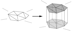
(a) Replacing triangles with prisms

(b) Capping prisms with pillows

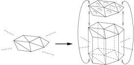
(c) The complete construction

(d) Triangulating prisms and pillows

Figure 5: Fattening a 2-manifold triangulation into a 3-manifold triangulation

If the original 2-manifold triangulation uses $2m$ triangles, the resulting 3-manifold triangulation uses $n=32m$ tetrahedra. Moreover, if two 3-manifold triangulations obtained using this construction are isomorphic, the original 2-manifold triangulations must also be isomorphic. The reason for this is as follows:

• Any isomorphism between two such 3-manifold triangulations must map triangular pillows to triangular pillows. This is because the internal vertex of each triangular pillow meets only two tetrahedra, and no other vertices under our construction have this property.

• By “flattening” the triangular pillows into 2-dimensional triangles, we thereby obtain an isomorphism between the underlying 2-manifold triangulations.

It follows that, for $n=32m$, we obtain a family of $\exp(\Omega(m\log m))=\exp(\Omega(n\log n))$ pairwise non-isomorphic 3-manifold triangulations.

This result is easily extended to $n\not\equiv 0\bmod 32$. Let $V_{n}$ denote the number of distinct isomorphism classes of 3-manifold triangulations of size $n$.

• Each triangulation of size $n$ has at least $n-1$ distinct 2-3 moves available (since any face joining two distinct tetrahedra defines a 2-3 move, and there are at least $n-1$ such faces).

• On the other hand, each triangulation of size $n+1$ has at most $6(n+1)$ distinct 3-2 moves available (since each 3-2 move is defined by an edge that meets three distinct tetrahedra, and the triangulation has at most $6(n+1)$ edges in total).

It follows that $V_{n+1}\geq V_{n}\cdot\frac{n-1}{6(n+1)}\geq V_{n}/18$ for any $n>1$. This gives $V_{32m+k}\geq V_{32m}/18^{31}$ for sufficiently large $m$ and all $0\leq k<32$, and so we obtain $V_{n}\in\exp(\Omega(n\log n))$ with no restrictions on $n$. ∎

Remark.

Of course, we expect that $V_{n+1}\gg V_{n}$ (and indeed we see this in the census). The bounds that we use to show $V_{n+1}\geq V_{n}/18$ in the proof above are very loose, but they are sufficient for the asymptotic result that we seek.

3.2 Isomorphism signatures

To construct the arcs of a Pachner graph, we begin at a node—that is, a 3-manifold triangulation $\mathcal{T}$—and perform Pachner moves. Our main difficulty is determining the endpoints of the arcs: each Pachner move results in a new triangulation $\mathcal{T}^{\prime}$, and we must determine which node of the graph represents $\mathcal{T}^{\prime}$.

A naïve approach might be to search through all nodes at the appropriate level of the Pachner graph and test each triangulation for isomorphism with $\mathcal{T}^{\prime}$. However, this is infeasible: although isomorphism testing is fast (as we prove in Corollary 3.5), the sheer number of nodes at level $n$ of the graph is too large (as shown by Theorem 3.1).

What we need is a property of the triangulation $\mathcal{T}^{\prime}$ that is easy to compute, and that uniquely defines the isomorphism class of $\mathcal{T}^{\prime}$. This property can be used as the key in a data structure with fast insertion and fast lookup (such as a hash table or a red-black tree), and by computing this property we can quickly jump to the relevant node of the graph.

Here we define such a property, which we call the isomorphism signature of a triangulation. In Theorem 3.3 we show that isomorphism signatures uniquely define isomorphism classes, and in Theorem 3.4 we show that they are small to store and fast to compute.

A labelling of a triangulation of size $n$ involves: (i) numbering its tetrahedra from 0 to $n-1$ inclusive, and (ii) numbering the four vertices of each tetrahedron from 0 to 3 inclusive. We also label the four faces of each tetrahedron from 0 to 3 inclusive so that face $i$ is opposite vertex $i$. A key ingredient of isomorphism signatures is canonical labellings, which we define as follows.

Definition (Canonical labelling).

Given a labelling of a triangulation of size $n$, let $A_{t,f}$ denote the tetrahedron glued to face $f$ of tetrahedron $t$ (so that $A_{t,f}\in\{0,\ldots,n-1\}$ for all $t=0,\ldots,n-1$ and $f=0,\ldots,3$). The labelling is canonical if, when we write out the sequence $A_{0,0},A_{0,1},A_{0,2},A_{0,3},\allowbreak A_{1,0},\ldots,A_{n-1,3}$, the following properties hold:

1. For each $1\leq i<j$, tetrahedron $i$ first appears before tetrahedron $j$ first appears.

2. For each $i\geq 1$, suppose tetrahedron $i$ first appears as the entry $A_{t,f}=i$. Then the corresponding gluing uses the identity map: face $f$ of tetrahedron $t$ is glued to face $f$ of tetrahedron $i$ so that vertex $v$ of tetrahedron $t$ maps to vertex $v$ of tetrahedron $i$ for each $v\neq f$.

As an example, consider the triangulation of size $n=3$ described by Table 2. This table lists the precise gluings of tetrahedron faces. For instance, the second cell in the bottom row indicates that face 1 of tetrahedron 2 is glued to tetrahedron 1, in such a way that vertices $0,2,3$ of tetrahedron 2 map to vertices $3,1,2$ of tetrahedron 1 respectively. This same gluing can be seen from the other direction by examining the first cell in the middle row.

	Face 0	Face 1	Face 2	Face 3
	Vertices 123	Vertices 023	Vertices 013	Vertices 012
Tet. 0	Tet. 0:   120	Tet. 1:   023	Tet. 2:   013	Tet. 0:   312
Tet. 1	Tet. 2:   230	Tet. 0:   023	Tet. 1:   012	Tet. 1:   013
Tet. 2	Tet. 2:   012	Tet. 1:   312	Tet. 0:   013	Tet. 2:   123

Table 2: The tetrahedron face gluings for an example 3-tetrahedron triangulation

It is simple to see that the labelling for this triangulation is canonical. The sequence $A_{0,0},\ldots,A_{n-1,3}$ is $0,1,2,0,\allowbreak 2,0,1,1,\allowbreak 2,1,0,2$ (reading tetrahedron numbers from left to right and then top to bottom in the table), and tetrahedron 1 first appears before tetrahedron 2 as required. Looking closer, the first appearance of tetrahedron 1 is in the second cell of the top row where vertices $0,2,3$ map to $0,2,3$, and the first appearance of tetrahedron 2 is in the subsequent cell where vertices $0,1,3$ map to $0,1,3$. In both cases the gluings use the identity map.

Lemma 3.2.

For any triangulation $\mathcal{T}$ of size $n$, there are precisely $24n$ canonical labellings of $\mathcal{T}$, and these can be enumerated in $O(n^{2}\log n)$ time.

Proof.

For $n=1$ the result is trivial, since all $24=4!$ possible labellings are canonical. For $n>1$ we observe that, if we choose (i) any one of the $n$ tetrahedra to label as tetrahedron 0, and (ii) any one of the $24$ possible labellings of its four vertices, then there is one and only one way to extend these choices to a canonical labelling of $\mathcal{T}$.

To see this, we can walk through the list of faces $F_{0,0},F_{0,1},F_{0,2},F_{0,3},F_{1,0},\ldots,F_{n-1,3}$, where $F_{t,i}$ represents face $i$ of tetrahedron $t$. The first face amongst $F_{0,0},\ldots,F_{0,3}$ that is joined to an unlabelled tetrahedron must in fact be joined to tetrahedron 1 using the identity map. This allows us to deduce tetrahedron 1 as well as the labels of its four vertices.

We inductively extend the labelling in this manner: once we have labelled tetrahedra $0,\ldots,k$ and their corresponding vertices, the first face amongst $F_{0,0},\ldots,F_{k,3}$ that is joined to an unlabelled tetrahedron must give us tetrahedron $k+1$ along with the labels for its four vertices (again using the identity map). The resulting labelling is canonical, and all of the labels can be deduced in $O(n\log n)$ time using a single pass through the list $F_{0,0},\ldots,F_{n-1,3}$. The $\log n$ factor is for manipulating tetrahedron labels, each of which requires $O(\log n)$ bits.

It follows that there are precisely $24n$ canonical labellings of $\mathcal{T}$, and that these can be enumerated in $O(n^{2}\log n)$ time using $24n$ iterations of the procedure described above. ∎

Definition (Isomorphism signature).

For any triangulation $\mathcal{T}$ of size $n$, enumerate all $24n$ canonical labellings of $\mathcal{T}$, and for each canonical labelling encode the full set of face gluings as a sequence of bits. We define the isomorphism signature to be the lexicographically smallest of these $24n$ bit sequences, and we denote this by $\sigma(\mathcal{T})$.

For the theoretical results in this section, it suffices to treat each sequence as a naïve bitwise encoding of a full table of face gluings (such as Table 2). In practical software settings however, we use a more compact alphanumeric representation with less redundancy, which we specify in full detail in the appendix.

Theorem 3.3.

Given two 3-manifold triangulations $\mathcal{T}$ and $\mathcal{T}^{\prime}$, we have $\sigma(\mathcal{T})=\sigma(\mathcal{T}^{\prime})$ if and only if $\mathcal{T}$ and $\mathcal{T}^{\prime}$ are isomorphic.

Proof.

It is clear that $\sigma(\mathcal{T})=\sigma(\mathcal{T}^{\prime})$ implies that $\mathcal{T}$ and $\mathcal{T}^{\prime}$ are isomorphic, since both signatures encode the same gluing data. Conversely, if $\mathcal{T}$ and $\mathcal{T}^{\prime}$ are isomorphic then their $24n$ canonical labellings are the same (though they might be enumerated in a different order). In particular, the lexicographically smallest canonical labellings will be identical; that is, $\sigma(\mathcal{T})=\sigma(\mathcal{T}^{\prime})$. ∎

Theorem 3.4.

Given a 3-manifold triangulation $\mathcal{T}$ of size $n$, the isomorphism signature $\sigma(\mathcal{T})$ has $O(n\log n)$ size and can be generated in $O(n^{2}\log n)$ time.

Proof.

To encode a full set of face gluings, at worst we require a table of gluing data such as Table 2, with $4n$ cells each containing four integers. Because some of these integers require $O(\log n)$ bits (the tetrahedron labels), it follows that the total size of $\sigma(\mathcal{T})$ is $O(n\log n)$.

The algorithm to generate $\sigma(\mathcal{T})$ is spelled out explicitly in its definition. The $24n$ canonical labellings of $\mathcal{T}$ can be enumerated in $O(n^{2}\log n)$ time (Lemma 3.2). Because a full set of face gluings has size $O(n\log n)$, we can encode the $24n$ bit sequences and select the lexicographically smallest in $O(n^{2}\log n)$ time, giving a time complexity of $O(n^{2}\log n)$ overall. ∎

This space complexity of $O(n\log n)$ is the best we can hope for, since Theorem 3.1 shows that the number of distinct isomorphism signatures for size $n$ triangulations grows like $\exp(\Theta(n\log n))$.

It follows from Theorems 3.3 and 3.4 that isomorphism signatures are ideal tools for constructing arcs in the Pachner graph, as explained at the beginning of this section. Moreover, the relevant definitions and results are easily extended to bounded and ideal triangulations (as described in the appendix). We finish with a simple but important consequence of our results:

Corollary 3.5.

Given two 3-manifold triangulations $\mathcal{T}$ and $\mathcal{T}^{\prime}$ each of size $n$, we can test whether $\mathcal{T}$ and $\mathcal{T}^{\prime}$ are isomorphic in $O(n^{2}\log n)$ time.

4 Analysing Pachner graphs

As discussed in the introduction, our focus is on one-vertex triangulations of closed prime orientable 3-manifolds and of the 3-sphere. We therefore direct our attention to the restricted Pachner graph $\mathscr{P}_{1}(\mathcal{M})$ of each such 3-manifold $\mathcal{M}$.

Definition (Base level).

For any closed 3-manifold $\mathcal{M}$, the base level $\beta_{1}(\mathcal{M})$ is the lowest non-empty level of the restricted Pachner graph $\mathscr{P}_{1}(\mathcal{M})$, excluding the isolated level 1. In other words, $\beta_{1}(\mathcal{M})$ is the smallest $n\geq 2$ for which there exists an $n$-tetrahedron, one-vertex triangulation of $\mathcal{M}$.

Lemma 4.1.

For any closed prime orientable 3-manifold $\mathcal{M}$ except for the lens spaces $L(4,1)$ and $L(5,2)$, the base level $\beta_{1}(\mathcal{M})$ is simply the size of a minimal triangulation of $\mathcal{M}$. If $\mathcal{M}=L(4,1)$ or $L(5,2)$, then $\beta_{1}(\mathcal{M})=3$. For the 3-sphere (which is not prime), $\beta_{1}(S^{3})=2$.

Proof.

From Table 1, there are only three one-vertex triangulations of closed 3-manifolds; these represent $S^{3}$, $L(4,1)$ and $L(5,2)$. The next smallest one-vertex triangulations of these manifolds in the census have sizes $\beta_{1}(S^{3})=2$, $\beta_{1}(L(4,1))=3$ and $\beta_{1}(L(5,2))=3$.

For any other closed prime orientable 3-manifold $\mathcal{M}$, either $\mathcal{M}=\mathbb{R}P^{3}$, $\mathcal{M}=L(3,1)$, or every minimal triangulation of $\mathcal{M}$ has one vertex [25]. In the latter case, the result follows immediately from the definition of $\beta_{1}(\mathcal{M})$. For both $\mathbb{R}P^{3}$ and $L(3,1)$ at least one minimal triangulation has one vertex, and so the result holds for these cases also. ∎

In this section, we analyse all $81\,800\,394$ triangulations of interest of size $n\leq 9$ in our census to obtain computer proofs of the following results:

Theorem 4.2 (Excess heights of simplification paths).

Let $\mathcal{M}$ be a closed prime orientable 3-manifold or the 3-sphere. From any node of $\mathscr{P}_{1}(\mathcal{M})$ at level $n$ where $\beta_{1}(\mathcal{M})<n\leq 9$, there is a simplification path of excess height $\leq 2$.

Theorem 4.3 (Lengths of simplification paths).

Let $\mathcal{M}$ be a closed prime orientable 3-manifold. From any node of $\mathscr{P}_{1}(\mathcal{M})$ at level $n$ where $\beta_{1}(\mathcal{M})<n\leq 9$, there is a simplification path of length $\leq 17$. For the 3-sphere, the bound is stronger: from any node of $\mathscr{P}_{1}(S^{3})$ at level $n$ where $\beta_{1}(S^{3})<n\leq 9$, there is some simplification path of length $\leq 9$.

Theorem 4.4 (Joining minimal triangulations).

Let $\mathcal{M}$ be a closed prime orientable 3-manifold that is not the lens space $L(3,1)$, and for which $\beta_{1}(\mathcal{M})\leq 9$. Then any two nodes at level $\beta_{1}(\mathcal{M})$ of $\mathscr{P}_{1}(\mathcal{M})$ are joined by a path of length $\leq 18$ and excess height $\leq 2$.

For the special case $L(3,1)$, there are precisely two nodes at level $\beta_{1}(L(3,1))=2$, and these are joined by a path of length $6$ and excess height $3$.

These results are astonishing, given Mijatović’s super-exponential bounds for the 3-sphere [29] and tower-of-exponential bounds for other manifolds [30, 31, 32]. Theorems 4.2 and 4.4 state that we can simplify triangulations or convert between minimal triangulations using at most two extra tetrahedra, and Theorems 4.3 and 4.4 state that we require very few Pachner moves. The 3-sphere results in particular have important algorithmic implications, which we discuss further in Section 6.

The algorithms behind these computer proofs are specialised, and use novel techniques to control the enormous time and space requirements. We return to these algorithmic issues shortly. In the meantime, some further comments on Theorems 4.2–4.4:

• We restrict our results to levels $n\leq 9$ because, even though we have census data for $n=10$ (see [8]), the sheer size of the census makes it infeasible to compute the necessary properties of the Pachner graphs. As a result, Theorems 4.2 and 4.3 cover $747$ distinct 3-manifolds with $\beta_{1}(\mathcal{M})<9$, and Theorem 4.4 covers $1900$ distinct 3-manifolds with $\beta_{1}(\mathcal{M})\leq 9$.

• Theorem 4.3 bounds the worst-case length of the shortest simplification path. If we bound the average length instead, the results are much smaller still: for the case $n=9$, this length is less than $1.89$ when averaged over all triangulations of $S^{3}$, and less than $1.91$ when averaged over all triangulations of closed prime orientable 3-manifolds. We present these average-case results in detail in Section 4.3.

• For arbitrary closed prime orientable 3-manifolds, the height results do not generalise. In Section 5, we construct (i) a triangulation of a graph manifold of size $n=10$ for which every simplification path has excess height $\geq 3$, and (ii) two minimal triangulations of a graph manifold with size $n=10$ where every path joining them has excess height $\geq 3$. For the case of the 3-sphere, no such counterexamples are known.

For the remainder of this section, we describe the algorithms behind Theorems 4.2–4.4, and present the experimental results in detail. Our algorithms are constrained by the following factors:

• Their time and space complexities must be close to linear in the number of nodes that they examine, due to the sheer size of the census.

• They cannot loop through all nodes in $\mathscr{P}_{1}(\mathcal{M})$, since the graph is infinite. They cannot even loop through all nodes at any level $n\geq 11$, since there are too many to enumerate.

• They cannot follow arbitrary breadth-first or depth-first searches through $\mathscr{P}_{1}(\mathcal{M})$, since the graph is infinite and can branch heavily in the upward direction.

Because of these limiting factors, we cannot run through the census and directly measure the shortest length or smallest excess height of any simplification path from each node. Instead we develop fast, localised algorithms that allow us to bound these quantities from above. To our delight, these upper bounds are extremely effective in practice.

A key optimisation in many of our algorithms comes from Theorem 4.5, which allows us to “reduce” sequences of Pachner moves to use fewer intermediate tetrahedra. We state and prove this theorem in Section 4.1. Following this, we present the individual algorithms:

• In Section 4.2 we give a fast algorithm based on union-find that bounds the heights of simplification paths. We run this algorithm over the census of 3-sphere triangulations, giving a computer proof for the 3-sphere case of Theorem 4.2.

• In Section 4.3 we describe a multiple-source breadth-first search algorithm that bounds lengths of simplification paths. By running this over the census of triangulations of the 3-sphere and closed prime orientable manifolds, we prove Theorem 4.3 as well as the outstanding closed prime orientable case of Theorem 4.2.

• In Section 4.4 we present algorithms that incorporate both breadth-first search and union-find techniques to study paths between nodes representing minimal triangulations. By running these algorithms over the census of minimal triangulations of closed prime orientable manifolds, we obtain a computer proof of Theorem 4.4.

• We finish in Section 4.5 with a discussion of how these algorithms can be parallelised effectively, along with explicit measurements of running time and memory use.

4.1 Reducing sequences of moves

The key idea behind reducing sequences of Pachner moves is that, in many cases, we can interchange pairs of consecutive 2-3 and 3-2 moves to become consecutive 3-2 and 2-3 moves instead, without changing the final triangulation. In the Pachner graph, this replaces a path segment from levels $n\to(n+1)\to n$ with a path segment from levels $n\to(n-1)\to n$: the length and endpoints of the overall path remain the same, and the excess height will either stay the same or decrease (depending on the heights of other segments of the path).

This type of interchange is not always possible. The purpose of Theorem 4.5 is to identify the “bad cases” where consecutive 2-3 and 3-2 moves cannot be interchanged, so that we can explicitly test for them in algorithms. In summary, we find that every bad 2-3 / 3-2 pair can be described by one of three “composite moves”. These composite moves are local modifications to a triangulation, much like the Pachner moves (though a little more complex), and are defined as follows.

Definition (Octahedron flip).

An octahedron flip, also known as a 4-4 move, involves four distinct tetrahedra surrounding a common edge of degree four. The move essentially rotates the configuration, replacing it with four new tetrahedra surrounding a new edge of degree four that points in a different direction, as illustrated in Figure 6.

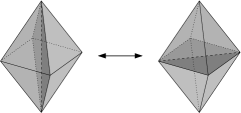
Figure 6: An octahedron flip

Definition (Pillow flip).

A quadrilateral pillow is formed from two distinct tetrahedra joined along two adjacent faces, as shown in Figure 7(a). A pillow flip is a move involving three tetrahedra: a quadrilateral pillow plus a third tetrahedron attached to one of its outer faces. The move essentially reflects the configuration, replacing it with a quadrilateral pillow plus a new tetrahedron attached to the opposite face instead.

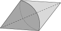
(a) A quadrilateral pillow

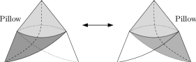
(b) Performing a pillow flip

Figure 7: A pillow flip

This move is illustrated in Figure 7(b), in which the pillows are shaded. In the left diagram the pillow is at the front, and the third tetrahedron is attached to its lower rear face. In the right diagram the pillow moves to the rear, and the third tetrahedron is attached to its lower front face instead.

Definition (Prism flip).

There are two types of prism flip, which we call types A and B. Both begin with three distinct tetrahedra joined to form a triangular prism, as illustrated in Figure 8(a). For the type A flip we also require that two rectangular faces of the prism are folded together, as shown in Figure 8(b); for type B we require that these same two rectangular faces be folded together with a $180^{\circ}$ twist instead. In both cases, the prism flip involves rotating the entire configuration so that the two triangular ends of the prism are interchanged, as shown in Figure 8(c).

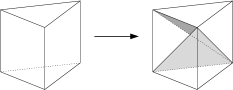
(a) A 3-tetrahedron triangular prism

(b) Folding two rectangular faces together

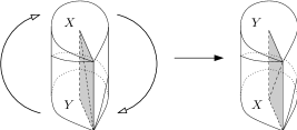
(c) Performing the move

Figure 8: A prism flip of type A

Remark.

It is easy to search for all possible octahedron, pillow or prism flips on a given triangulation, since each occurs around an edge of degree four, two or five respectively. We can simply search for edges of the correct degree, test for the necessary configuration of tetrahedra, and perform the flip if possible.

Note that there could be two different octahedron flips around the same degree four edge (corresponding to the two possible directions for the new edge that replaces it), and there could be four different pillow flips around the same degree two edge (corresponding to the four faces of the pillow to which the third tetrahedron might be attached). Around a degree five edge, there can only ever be one prism flip (if there is any at all).

Theorem 4.5.

Let $\mathcal{T}$ and $\mathcal{T}^{\prime}$ be 3-manifold triangulations, where $\mathcal{T}^{\prime}$ can be obtained from $\mathcal{T}$ by performing a 2-3 move followed by a 3-2 move. Then one of the following cases holds:

• $\mathcal{T}^{\prime}$ is isomorphic to $\mathcal{T}$;

• $\mathcal{T}^{\prime}$ can be obtained from $\mathcal{T}$ by performing a 3-2 move followed by a 2-3 move instead (i.e., using one fewer tetrahedron at the intermediate stage instead of one more);

• $\mathcal{T}^{\prime}$ can be obtained from $\mathcal{T}$ by performing either an octahedron flip, a pillow flip, or a prism flip.

Proof.

Suppose that we obtain $\mathcal{T}^{\prime}$ from $\mathcal{T}$ by:

1. performing a 2-3 move on two adjacent tetrahedra $\Delta_{1},\Delta_{2}$ of $\mathcal{T}$, giving the intermediate triangulation $\mathcal{I}$;

2. then performing a 3-2 move around the degree three edge $e$ of $\mathcal{I}$ to give $\mathcal{T}^{\prime}$.

If $e$ is not an edge of the original triangulation $\mathcal{T}$, then it must be created by the 2-3 move. Therefore the subsequent 3-2 move is the inverse of the original 2-3 move, and the final triangulation $\mathcal{T}^{\prime}$ is isomorphic to $\mathcal{T}$.

Suppose then that $e$ does belong to the original triangulation $\mathcal{T}$, but that $e$ is not an edge of either $\Delta_{1}$ or $\Delta_{2}$. This implies that the 2-3 move and the 3-2 move occur in “disjoint” regions of the triangulation: none of the tetrahedra involved in the 3-2 move are also involved in the 2-3 move. Therefore the 2-3 and 3-2 moves can be applied in either order, and we can obtain $\mathcal{T}^{\prime}$ from $\mathcal{T}$ by performing the 3-2 move followed by the 2-3 move instead.

Finally, suppose that $e$ is an edge of $\Delta_{1}$ and/or $\Delta_{2}$ in $\mathcal{T}$. Note that $e$ might not have degree three in $\mathcal{T}$, and it might appear as multiple edges of $\Delta_{1}$ and/or $\Delta_{2}$. However, in the intermediate triangulation $\mathcal{I}$ (after the initial 2-3 move), it must have degree three and it must belong to three distinct tetrahedra.

Up to isomorphism, there are 13 possible ways that $e$ can appear in $\Delta_{1}$ and/or $\Delta_{2}$ subject to these constraints. These fall into five basic patterns, as illustrated in Figure 9. Cases 1, 2 and 4 require additional tetrahedra in order to meet the degree three requirement (these extra tetrahedra are also pictured). Cases 2, 3 and 5 each have several different subcases, according to the specific orientations of $e$ in each tetrahedron and the different ways in which tetrahedron faces can be glued together.

Figure 9: Possible locations for the edge $e$ in $\mathcal{T}$

Cases 1 and 4 are simple to analyse. Figure 10 shows the corresponding configurations in $\mathcal{T}$ with the extra tetrahedra glued in: these are the initial configurations for an octahedron flip and a pillow flip respectively. By following the details of the 2-3 move on $\Delta_{1}$ and $\Delta_{2}$ followed by the 3-2 move around $e$, we indeed find that these moves perform a single octahedron flip in case 1, and a single pillow flip in case 4.

Figure 10: The full configurations in $\mathcal{T}$ for cases 1 and 4

For case 2, there are four possible configurations up to isomorphism. These are shown in Figure 11, again with the extra tetrahedron glued in. These four subcases correspond to different possible orientations of $e$ in each tetrahedron (indicated in the diagram by the bold arrowheads) and different possible choices for which faces are glued together (indicated by the white arrows and the shading on the faces).

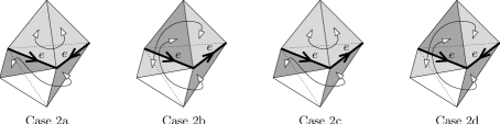
Figure 11: The four possible configurations for case 2

Subcase 2a is precisely the initial configuration for a prism flip of type A (the two shaded triangles on the left form one rectangular face of the prism, and the two shaded triangles on the right form another). Likewise, subcase 2b is the initial configuration for a prism flip of type B (the different gluings describe a $180^{\circ}$ twist before folding these rectangles together). In each case, the 2-3 and 3-2 move together carry out the corresponding prism flip.

Subcases 2c and 2d both produce non-orientable triangulations. More importantly, each contains a vertex $V$ with a non-orientable link—in other words, any small regular neighbourhood of $V$ is non-orientable. For subcase 2c, this vertex is at the top of the diagram, and for subcase 2d it is the vertex at the centre of the diagram. No such vertex can appear in a 3-manifold triangulation, and so subcases 2c and 2d can never occur.

In case 3, all eight faces of $\Delta_{1}$ and $\Delta_{2}$ are glued together in pairs. Since the triangulation $\mathcal{T}$ is connected, this means that $\mathcal{T}$ contains only these two tetrahedra: if $n>2$ then this case can never occur at all. Even if $n=2$, the triangulation is not of interest to us, since $\mathcal{T}$ will contain two distinct vertices and so will not feature in any restricted Pachner graph.

Nevertheless, we summarise case 3 with $n=2$ for completeness. Here there are five subcases up to isomorphism, again depending on the possible orientations of $e$ and choices for how the the tetrahedron faces are glued together. Three of these subcases give non-orientable vertex links as before, and so cannot occur. Of the final two subcases, one gives $\mathcal{T}$ as the unique two-vertex, two-tetrahedron triangulation of $S^{3}$, and the other gives the unique two-vertex, two-tetrahedron triangulation of the lens space $L(3,1)$. In both subcases, the 2-3 and 3-2 move together produce a triangulation that is isomorphic to the original.

This leaves case 5. Here there are two possible configurations in $\mathcal{T}$ up to isomorphism, as illustrated in Figure 12 (in both diagrams, the top left face at the front is glued to the upper face at the rear, and the top right face at the front is glued to the lower face at the rear). Subcase 5a gives an orientable triangulation (to be precise, a $(1,3,4)$ layered solid torus [19]), and following through the 2-3 and 3-2 moves shows once again that the resulting triangulation is isomorphic to the original. Subcase 5b gives a non-orientable triangulation in which the top left edge is identified with itself in reverse, and so this subcase can never occur. ∎

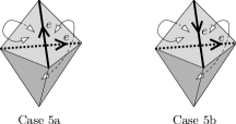
Figure 12: The two possible configurations for case 5

4.2 Bounding excess heights

Our first algorithm computes bounds $H_{n}(\mathcal{M})$ for a given 3-manifold $\mathcal{M}$ and a given level $n>\beta_{1}(\mathcal{M})$ so that, from every node at level $n$ of the graph $\mathscr{P}_{1}(\mathcal{M})$, there is a simplification path of excess height $\leq H_{n}(\mathcal{M})$. By running this algorithm, we explicitly compute these bounds for the case $\mathcal{M}=S^{3}$, for each $n$ in the range $2<n\leq 9$.

The general idea is to begin with the set of all nodes at level $n$, and repeatedly expand into higher levels using 2-3 moves only until all of the original nodes are connected together. If the bound $H_{n}(\mathcal{M})$ is tight (as we find in practice for the 3-sphere), this method of “upward expansion” saves significant time and memory by enumerating only a fraction of the higher levels $\ell>n$ (each of which contains far more nodes than the initial level $n$).

Algorithm 4.6 (Computing $H_{n}$).

This algorithm runs by progressively building a finite subgraph $G\subset\mathscr{P}_{1}(\mathcal{M})$. At all times we keep track of the number of distinct components of $G$ (denoted by $c$) and the maximum level of any node in $G$ (denoted by $\ell$).

1. Initialise $G$ to all of level $n$ of $\mathscr{P}_{1}(\mathcal{M})$. This means that $G$ has no arcs, the number of components $c$ is just the number of nodes at level $n$, and the maximum level is $\ell=n$.

2. While $c>1$, expand the graph as follows:

   1. Construct all arcs from nodes in $G$ at level $\ell$ to (possibly new) nodes in $\mathscr{P}_{1}(\mathcal{M})$ at level $\ell+1$. Insert these arcs and their endpoints into $G$.

   2. Update the number of components $c$, and increment $\ell$ by one.

3. Once we have $c=1$, output the final bound $H_{n}(\mathcal{M})=\ell-n$ and terminate.

In step 2(a) we construct arcs by performing 2-3 moves, and in step 2(b) we use union-find to update the number of components in small time complexity.

It is clear that Algorithm 4.6 is correct for any $n>\beta_{1}(\mathcal{M})$: once we have $c=1$ the subgraph $G$ is connected, which means it contains a path from any node at level $n$ to any other node at level $n$. Because $n>\beta_{1}(\mathcal{M})$, Theorem 2.1 shows that at least one such node allows a 3-2 move, and so any node at level $n$ has a simplification path of excess height $\leq\ell-n$.

However, it is not clear that Algorithm 4.6 terminates: it might be that every simplification path from some node at level $n$ passes through nodes that we never construct at higher levels $\ell>n$. Happily it does terminate for the 3-sphere for all $2<n\leq 9$, giving an output of $H_{n}(S^{3})=2$ each time, and thereby proving the 3-sphere case for Theorem 4.2. Table 3 shows how the number of components $c$ changes as the algorithm runs for each $n$.

$$\small\begin{array}[]{l|r|r|r|r|r|r|r}\mbox{Input level $n$}&3&4&5&6&7&8&9\\ \hline\cr\mbox{Value of $c$ when $\ell=n$}&20&128&1\,297&13\,660&169\,077&2\,142\,197&28\,691\,150\\ \mbox{Value of $c$ when $\ell=n+1$}&8&50&196&1\,074&7\,784&64\,528&557\,428\\ \mbox{Value of $c$ when $\ell=n+2$}&1&1&1&1&1&1&1\\ \hline\cr\mbox{Final bound $H_{n}(S^{3})$}&\mathbf{2}&\mathbf{2}&\mathbf{2}&\mathbf{2}&\mathbf{2}&\mathbf{2}&\mathbf{2}\end{array}$$

Table 3: Running Algorithm 4.6 on the 3-sphere for all levels $2<n\leq 9$

Lemma 4.7.

If Algorithm 4.6 outputs $H_{n}(\mathcal{M})\leq 2$, then this bound is tight. In other words, $H_{n}(\mathcal{M})=\max_{\nu}\min_{p}\mathrm{excess~{}height}(p)$, where $\nu$ ranges over all nodes at level $n$ of $\mathscr{P}_{1}(\mathcal{M})$, and where $p$ ranges over all simplification paths that begin at $\nu$.

Proof.

The result is trivial for $H_{n}(\mathcal{M})\leq 1$. Suppose then that $H_{n}(\mathcal{M})=2$ and this bound is not tight; that is, $\max_{\nu}\min_{p}\mathrm{excess~{}height}(p)\leq 1$. When Algorithm 4.6 processes level $\ell=n+1$, it effectively enumerates all paths in $\mathscr{P}_{1}(\mathcal{M})$ that stay between levels $n$ and $n+1$, since every arc between these levels emanates from one of our starting nodes at level $n$. Therefore Algorithm 4.6 would terminate at level $\ell\leq n+1$ and output $H_{n}(\mathcal{M})\leq 1$ instead, a contradiction. ∎

As a result, our bounds $H_{n}(S^{3})=2$ for $2<n\leq 9$ are all tight. Note that Lemma 4.7 does not work in the opposite direction: it is possible to have $\max_{\nu}\min_{p}\mathrm{excess~{}height}(p)=2$ but $H_{n}(\mathcal{M})>2$, since the optimal path might bounce around between levels $n+1$ and $n+2$, using intermediate nodes that never appear in our subgraph $G$.

It is straightforward to show that the space and time complexities of Algorithm 4.6 are linear and log-linear respectively in the number of nodes in $G$ (other small polynomial factors in $n$ and $\ell$ also appear). Nevertheless, the memory requirements for $n=8$ were found to be extremely large in practice ($\sim$30 GB): by the time the algorithm terminated at level $\ell=10$, we had visited $185\,697\,092$ nodes in total. For $n=9$ the memory requirements were too large for the algorithm to run (estimated at 400–500 GB), and so a two-phase approach was necessary:

Algorithm 4.8 (Two-phase algorithm for computing $H_{n}$).

The following algorithm will either compute the same bound $H_{n}(\mathcal{M})$ as Algorithm 4.6, or will terminate with no result. Once again, we progressively build a finite subgraph $G\subset\mathscr{P}_{1}(\mathcal{M})$ and track the number of connected components $c$.

1. Initialise $G$ to all of level $n$ of $\mathscr{P}_{1}(\mathcal{M})$, as before.

2. Construct all arcs from nodes in $G$ at level $n$ to (possibly new) nodes in $\mathscr{P}_{1}(\mathcal{M})$ at level $n+1$. Insert these arcs and their endpoints into $G$, and update $c$ accordingly.

   If $c=1$ then output $H_{n}(\mathcal{M})=1$ and terminate.

3. From each node $\nu$ at level $n+1$, try all possible octahedron flips, pillow flips and prism flips. Let $\nu^{\prime}$ be the endpoint of such a flip (so $\nu^{\prime}$ is also a node at level $n+1$). If $\nu^{\prime}\in G$ then merge the components and decrement $c$ if necessary. Otherwise do nothing (since $\nu^{\prime}$ would never have been constructed in the previous algorithm).

   If $c=1$ then output $H_{n}(\mathcal{M})=2$ and terminate; otherwise terminate with no result.

In essence, we use the old Algorithm 4.6 for the transition from level $n\to n+1$, but then we use Theorem 4.5 to “simulate” the transition from level $n+1\to n+2$. We only need to consider octahedron, pillow and prism flips in step 3 because, by Theorem 4.5, if two nodes $\nu,\nu^{\prime}\in G$ at level $n+1$ have arcs to some common node $\nu^{\prime\prime}$ at level $n+2$, then either $\nu$ and $\nu^{\prime}$ are related by such a flip, or else $\nu$ and $\nu^{\prime}$ must already be connected in $G$.

It follows that, if this two-phase approach does output a result, it will always be the same result as Algorithm 4.6. The key advantage of this two-phase method is a much smaller memory footprint (since it does not store any nodes at level $n+2$). The main disadvantage is that it cannot move on to level $n+3$ if required, and so if $H_{n}(\mathcal{M})>2$ then it cannot output any result at all.

Of course by the time we reach $n=9$ for the 3-sphere, there are reasons to suspect that $H_{n}(S^{3})=2$ (following the pattern for $3\leq n\leq 8$), and so this two-phase method seems a reasonable—and ultimately successful—approach. For $n=9$ the memory consumption was $\sim$52 GB, which was (just) within the capabilities of the host machine.

4.3 Bounding path lengths

Our next task is to compute bounds $L_{n}(\mathcal{M})$ for a given 3-manifold $\mathcal{M}$ and a given level $n>\beta_{1}(\mathcal{M})$ so that, from every node at level $n$ of $\mathscr{P}_{1}(\mathcal{M})$, there is some simplification path of length $\leq L_{n}(\mathcal{M})$. This time we compute $L_{n}$ for all $n\leq 9$ and all closed prime orientable 3-manifolds $\mathcal{M}$ in the census, as well as for the case $\mathcal{M}=S^{3}$.

It is infeasible to perform arbitrary breadth-first searches through $\mathscr{P}_{1}(\mathcal{M})$, and so we restrict such searches using two techniques:

1. we only search within levels $n$, $n+1$ and $n+2$, and we only explicitly store nodes in levels $n$ and $n+1$;

2. we only visit level $n+2$ when absolutely necessary, as described by Theorem 4.5.

Of course (i) is only effective if there is a simplification path of excess height $\leq 2$. The results of the previous section show that this is true for $\mathcal{M}=S^{3}$ and $n\leq 9$, and give us hope that it holds for other manifolds also. Although the shortest simplification paths might pass through levels $n+3$ or above (and so our bounds $L_{n}(\mathcal{M})$ might not be tight), the time and space savings obtained by avoiding these higher levels (which grow at a super-exponential rate) are enormous.

In the algorithm below, we refer to steps as the quantity minimised by the breadth-first search. Since each octahedron, pillow or prism flip involves two Pachner moves, we use a modified breadth-first search for weighted graphs in which some arcs are counted as one step and some arcs are counted as two. Such modifications are standard, and we do not go into details here.

Algorithm 4.9 (Computing $L_{n}$).

First identify the set $S$ of all nodes at level $n$ of $\mathscr{P}_{1}(\mathcal{M})$ that have an arc running down to level $n-1$. Then conduct a multiple-source breadth-first search across levels $n$ and $n+1$, beginning with $S$ as the set of sources, where the steps in this breadth-first search are as follows:

• all arcs between levels $n$ and $n+1$ of $\mathscr{P}_{1}(\mathcal{M})$, each of which is treated as one step;

• all octahedron, pillow and prism flips at level $n+1$ of $\mathscr{P}_{1}(\mathcal{M})$, each of which is treated as two steps.

If $s$ is the maximum number of steps required to reach any node in level $n$ from the initial source set $S$, then output the final bound $L_{n}(\mathcal{M})=s+1$. If some nodes at level $n$ are never reached, then output $L_{n}(\mathcal{M})=\infty$ instead.

This time the algorithm always terminates, since levels $n$ and $n+1$ are finite. The algorithm is also correct, because each source node in $S$ has a simplification path of length 1, and each step in the breadth-first search corresponds to a single 2-3 or 3-2 move. The space and time complexities are linear and log-linear respectively in the number of nodes in levels $n$ and $n+1$ (again with further small polynomial factors in $n$).

We can make some observations on the tightness of the bounds $L_{n}(\mathcal{M})$:

Lemma 4.10.

The bound $L_{n}(\mathcal{M})$ computed by Algorithm 4.9 is finite if and only if every node at level $n$ of $\mathscr{P}_{1}(\mathcal{M})$ has a simplification path of excess height $\leq 2$.

If this bound is finite, then it is also tight if we restrict our attention to only simplification paths of excess height $\leq 2$. That is, $L_{n}(\mathcal{M})=\max_{\nu}\min_{p}\mathrm{length}(p)$, where $\nu$ ranges over all nodes at level $n$ of $\mathscr{P}_{1}(\mathcal{M})$, and where $p$ ranges over all simplification paths of excess height $\leq 2$ that begin at $\nu$.

The proof follows directly from the structure of the breadth-first search and from Theorem 4.5, which shows that every step up into level $n+2$ is either part of an octahedron, pillow or prism flip, or else can be replaced with a step down into level $n$ instead.

For the 3-sphere, Table 4 shows how the breadth-first search progresses for each $n$ in the range $2<n\leq 9$. Each cell of this table counts only nodes at level $n$ of $\mathscr{P}_{1}(S^{3})$, not “intermediate nodes” at the higher level $n+1$. For each $n$ the algorithm outputs a final bound of $L_{n}(S^{3})=7$ or $9$, proving the 3-sphere case of Theorem 4.3.

$$\small\begin{array}[]{l|r|r|r|r|r|r|r}\mbox{Input level $n$}&3&4&5&6&7&8&9\\ \hline\cr\mbox{Nodes in $S$}&3&46&504&6\,975&91\,283&1\,300\,709&18\,361\,866\\ \mbox{Nodes 2 steps from $S$}&8&38&466&4\,315&54\,698&624\,144&8\,044\,998\\ \mbox{Nodes 4 steps from $S$}&7&43&309&2\,299&22\,634&213\,345&2\,255\,191\\ \mbox{Nodes 6 steps from $S$}&2&1&18&71&462&3988&29\,054\\ \mbox{Nodes 8 steps from $S$}&&&&&&11&41\\ \hline\cr\mbox{Total level $n$ nodes found}&20&128&1\,297&13\,660&169\,077&2\,142\,197&28\,691\,150\\ \mbox{Total level $n$ nodes missing}&0&0&0&0&0&0&0\\ \hline\cr\mbox{Final bound $L_{n}$}&\mathbf{7}&\mathbf{7}&\mathbf{7}&\mathbf{7}&\mathbf{7}&\mathbf{9}&\mathbf{9}\end{array}$$

Table 4: Running Algorithm 4.9 over the 3-sphere

Observation 4.11.

The bounds $L_{n}$ in Table 4 are tight even if we consider all simplification paths (not just those with excess height $\leq 2$).

Proof.

For $n\leq 7$ this follows immediately from Lemma 4.10, since any simplification path of excess height $\geq 3$ must have length $\geq 7$. For $n=8$ or $9$, the bounds are likewise tight unless all $11$ or $41$ triangulations respectively that are eight steps from $S$ have a simplification path of length $\leq 8$ and excess height $\geq 3$. The only way to construct such a path is using three 2-3 moves followed by four 3-2 moves. We can enumerate all such combinations of moves by computer, and we find in all 11 cases for $n=8$ and in 40 of the 41 cases for $n=9$ that no such path exists. ∎

Table 5 shows the corresponding results for arbitrary closed prime orientable 3-manifolds. Each cell in this table is a sum over all such manifolds $\mathcal{M}$ with $\beta_{1}(\mathcal{M})<n$, except for the final row which lists the largest bound $L_{n}(\mathcal{M})$ amongst all such manifolds. In every case we have $L_{n}(\mathcal{M})\leq 17$, proving the closed prime orientable case of Theorem 4.3.

$$\small\begin{array}[]{l|r|r|r|r|r|r|r}\mbox{Input level $n$}&3&4&5&6&7&8&9\\ \hline\cr\mbox{Nodes in $S$}&8&80&931&11\,380&151\,278&2\,098\,537&30\,082\,708\\ \mbox{Nodes 2 steps from $S$}&2&73&682&7\,078&80\,998&991\,080&12\,579\,745\\ \mbox{Nodes 4 steps from $S$}&8&72&483&4\,163&38\,253&391\,516&4\,185\,195\\ \mbox{Nodes 6 steps from $S$}&1&13&44&324&2\,290&16\,714&131\,545\\ \mbox{Nodes 8 steps from $S$}&&&&12&69&427&2\,591\\ \mbox{Nodes 10 steps from $S$}&&&&&&12&51\\ \mbox{Nodes 12 steps from $S$}&&&&&&&13\\ \mbox{Nodes 14 steps from $S$}&&&&&&&\\ \mbox{Nodes 16 steps from $S$}&&&&&&&1\\ \hline\cr\mbox{Total level $n$ nodes found}&19&238&2\,140&22\,957&272\,888&3\,498\,286&46\,981\,849\\ \mbox{Total level $n$ nodes missing}&0&0&0&0&0&0&0\\ \hline\cr\mbox{Maximum bound $L_{n}$}&\mathbf{7}&\mathbf{7}&\mathbf{7}&\mathbf{9}&\mathbf{9}&\mathbf{11}&\mathbf{17}\end{array}$$

Table 5: Running Algorithm 4.9 over arbitrary closed prime orientable 3-manifolds

Furthermore, by Lemma 4.10, an immediate consequence of these results is as follows. For any closed prime orientable 3-manifold $\mathcal{M}$, from any node at level $n$ of $\mathscr{P}_{1}(\mathcal{M})$ where $\beta_{1}(\mathcal{M})<n\leq 9$, there is a simplification path with excess height $\leq 2$. This proves the remaining closed prime orientable case of Theorem 4.2.

It is clear from Tables 4 and 5 that most nodes at level $n$ are very close to the source set $S$, and only a tiny fraction require all $L_{n}(\mathcal{M})$ steps. This prompts us to consider average lengths of simplification paths. In particular, we consider the following two quantities:

• $\sigma_{n}=\mathrm{avg}_{\nu}\min_{p}\mathrm{length}(p)$, where $\nu$ ranges over all nodes at level $n$ of $\mathscr{P}_{1}(S^{3})$, and where $p$ ranges over all simplification paths that begin at $\nu$;

• $\pi_{n}=\mathrm{avg}_{\nu}\min_{p}\mathrm{length}(p)$, where $\nu$ ranges over all nodes at level $n$ of all graphs $\mathscr{P}_{1}(\mathcal{M})$ for closed prime orientable 3-manifolds $\mathcal{M}$ with $\beta_{1}(\mathcal{M})<n$, and again $p$ ranges over all simplification paths that begin at $\nu$.

In other words, if we consider the shortest simplification path from each node, then $\sigma_{n}$ is the average path length over all size $n$ triangulations of the 3-sphere, and $\pi_{n}$ is the average path length over all size $n$ triangulations of closed prime orientable 3-manifolds.

By aggregating the figures in Tables 4 and 5, we can place upper bounds on $\sigma_{n}$ and $\pi_{n}$ respectively (since each node that is $k$ steps from the source set $S$ has a simplification path of length $\leq k+1$). These upper bounds are listed in Table 6 (all numbers are rounded up).

$$\small\begin{array}[]{l|r|r|r|r|r|r|r}\mbox{Input level $n$}&3&4&5&6&7&8&9\\ \hline\cr\mbox{Upper bound on $\sigma_{n}$}&3.80&2.99&2.76&2.34&2.20&2.00&1.89\\ \mbox{(3-sphere triangulations)}&&&&&&&\\ \hline\cr\mbox{Upper bound on $\pi_{n}$}&3.22&3.16&2.67&2.44&2.21&2.05&1.91\\ \mbox{(closed prime orientable 3-manifolds)}&&&&&&&\\ \end{array}$$

Table 6: Bounding the average lengths of simplification paths

These averages are remarkably small, and more importantly, they appear to decrease with $n$: although the worst-case paths become longer, such pathological cases become very rare very quickly. This has interesting implications for generic-case complexity, which we return to in Section 6. Figure 13 gives a graphical summary of these worst-case and average-case bounds.

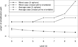
Figure 13: Summary of bounds on lengths of simplification paths

4.4 Connecting minimal triangulations

Our final algorithms examine paths that connect different nodes at the base level $\beta_{1}(\mathcal{M})$ of $\mathscr{P}_{1}(\mathcal{M})$. Recall from Lemma 4.1 that, for most closed prime orientable 3-manifolds $\mathcal{M}$, these are the nodes that correspond to minimal triangulations of $\mathcal{M}$.

In particular, these algorithms compute bounds $H_{\mathrm{min}}(\mathcal{M})$ and $L_{\mathrm{min}}(\mathcal{M})$ for a given 3-manifold $\mathcal{M}$ so that, between any two nodes at level $\beta_{1}(\mathcal{M})$ of $\mathscr{P}_{1}(\mathcal{M})$, there is a path of excess height $\leq H_{\mathrm{\min}}(\mathcal{M})$, and a (possibly different) path of length $\leq L_{\mathrm{\min}}(\mathcal{M})$.

Here the running time and memory use are less critical: because the census contains so few minimal triangulations of closed prime orientable 3-manifolds (just 4472 for $n\leq 9$), we can afford to search exhaustively through entire levels of $\mathscr{P}_{1}(\mathcal{M})$ as long as these levels do not grow too high above $\beta_{1}(\mathcal{M})$.

Algorithm 4.12 (Computing $H_{\mathrm{min}}$).

As before, this algorithm runs by progressively building a finite subgraph $G\subset\mathscr{P}_{1}(\mathcal{M})$. We track the number of distinct components of $G$ (denoted by $c$) and the maximum level of any node in $G$ (denoted by $\ell$).

1. Initialise $G$ to all of level $\beta_{1}(\mathcal{M})$ of $\mathscr{P}_{1}(\mathcal{M})$, set the number of components $c$ to the number of nodes at level $\beta_{1}(\mathcal{M})$, and set the maximum level $\ell=\beta_{1}(\mathcal{M})$.

2. While $c>1$, expand $G$ using a multiple-source breadth-first search as follows:

   • Maintain a queue of nodes to be processed. Initially this queue should contain all nodes at level $\ell$ in $G$ (these are the multiple source nodes).

   • To process a node $\nu$, follow all arcs from $\nu$ in $\mathscr{P}_{1}(\mathcal{M})$ whose endpoints lie in levels $\leq\ell+1$, and add these arcs and their endpoints to $G$ if not already present. Each new node that is added to $G$ must also be pushed onto the queue for processing. Decrement $c$ each time a new arc joins two disconnected components of $G$.

   • Once the queue is empty (i.e., there are no more nodes to process), increment $\ell$.

3. Once we have $c=1$, output the final bound $H_{\mathrm{min}}(\mathcal{M})=\ell-\beta_{1}(\mathcal{M})$ and terminate.

As in Algorithm 4.6, we enumerate arcs from a node $\nu$ by performing 2-3 and 3-2 moves, and we track connected components of $G$ using union-find.

It is clear from the structure of the breadth-first search that, at each stage of the algorithm, the subgraph $G$ contains precisely those nodes that can be reached from level $\beta_{1}(\mathcal{M})$ of $\mathscr{P}_{1}(\mathcal{M})$ using a path that never travels above level $\ell$. We can therefore conclude:

Lemma 4.13.

The bound $H_{\mathrm{min}}(\mathcal{M})$ output by Algorithm 4.12 is tight. That is, $H_{\mathrm{min}}(\mathcal{M})=\max_{\nu_{1},\nu_{2}}\min_{p}\mathrm{excess~{}height}(p)$, where $\nu_{1}$ and $\nu_{2}$ range over all nodes at level $\beta_{1}(\mathcal{M})$ of $\mathscr{P}_{1}(\mathcal{M})$, and where $p$ ranges over all paths in $\mathscr{P}_{1}(\mathcal{M})$ from $\nu_{1}$ to $\nu_{2}$.

Running this over all 1900 closed prime orientable 3-manifolds $\mathcal{M}$ with $\beta_{1}(\mathcal{M})\leq 9$, we find that $H_{\mathrm{min}}(\mathcal{M})\leq 2$ in every case but one. The exception is one of the smallest cases in the census: the lens space $L(3,1)$, with $\beta_{1}(L(3,1))=2$ and final bound $H_{\mathrm{min}}(L(3,1))=3$. Table 7 shows a detailed breakdown of the results, which together constitute a computer proof of the excess height results from Theorem 4.4. Note that the manifolds in the table with $H_{\mathrm{min}}(\mathcal{M})=0$ are those with only one node at level $\beta_{1}(\mathcal{M})$ of $\mathscr{P}_{1}(\mathcal{M})$.

$$\small\begin{array}[]{l|r|r|r|r|r|r|r|r||r}\mbox{Base level $\beta_{1}(\mathcal{M})$}&2&3&4&5&6&7&8&9&\mbox{Total}\\ \hline\cr\mbox{Manifolds with $H_{\mathrm{min}}(\mathcal{M})=0$}&6&7&13&23&47&106&235&575&1\,012\\ \mbox{Manifolds with $H_{\mathrm{min}}(\mathcal{M})=1$}&&1&1&7&20&52&156&455&692\\ \mbox{Manifolds with $H_{\mathrm{min}}(\mathcal{M})=2$}&&1&&1&7&17&45&124&195\\ \mbox{Manifolds with $H_{\mathrm{min}}(\mathcal{M})=3$}&1&&&&&&&&1\\ \hline\cr\mbox{Manifolds with $H_{\mathrm{min}}(\mathcal{M})\geq 4$}&0&0&0&0&0&0&0&0&0\\ \end{array}$$

Table 7: Bounding excess heights of paths between nodes at level $\beta_{1}(\mathcal{M})$

To bound path lengths, we adopt a similar strategy to that for simplification paths: because excess heights are typically bounded above by $H_{\mathrm{min}}(\mathcal{M})\leq 2$, we perform breadth-first searches that stay within levels $\beta_{1}(\mathcal{M})$, $\beta_{1}(\mathcal{M})+1$ and $\beta_{1}(\mathcal{M})+2$. Once again, we use octahedron, pillow and prism flips to avoid explicitly stepping into level $\beta_{1}(\mathcal{M})+2$. The full algorithm is as follows.

Algorithm 4.14 (Computing $L_{\mathrm{min}}$).

For each node $\nu$ at level $\beta_{1}(\mathcal{M})$, run a single-source breadth-first search from $\nu$ across levels $\beta_{1}(\mathcal{M})$ and $\beta_{1}(\mathcal{M})+1$ of $\mathscr{P}_{1}(\mathcal{M})$. The steps in this breadth-first search are as follows:

• all arcs between levels $\beta_{1}(\mathcal{M})$ and $\beta_{1}(\mathcal{M})+1$, each of which is treated as one step;

• all octahedron, pillow and prism flips at level $\beta_{1}(\mathcal{M})+1$, each of which is treated as two steps.

Let $d(\nu)$ denote the maximum number of steps required to reach any node at level $\beta_{1}(\mathcal{M})$ from the source $\nu$, or let $d(\nu)=\infty$ if some node at level $\beta_{1}(\mathcal{M})$ was never reached. After computing $d(\nu)$ for each source node $\nu$, output the final bound $L_{\mathrm{\min}}(\mathcal{M})=\max_{\nu}d(\nu)$.

This approach of running a separate breadth-first search from each node $\nu$ at level $\beta_{1}(\mathcal{M})$ is perhaps wasteful, but there are so few minimal triangulations in the census that its performance is adequate nonetheless.

As with Algorithm 4.9 for simplification paths, we can make some simple observations on the tightness of the bounds $L_{\mathrm{min}}(\mathcal{M})$. The following result is an immediate consequence of Theorem 4.5, the breadth-first search structure of Algorithm 4.14, and the tightness of the height bounds $H_{\mathrm{min}}(\mathcal{M})$ as shown by Lemma 4.13.

Lemma 4.15.

The bound $L_{\mathrm{min}}(\mathcal{M})$ that is computed by Algorithm 4.14 is finite if and only if $H_{\mathrm{min}}(\mathcal{M})\leq 2$. Moreover, if the bound $L_{\mathrm{\min}}(\mathcal{M})$ is finite, then it is also tight if we restrict our attention to paths of excess height $\leq 2$. That is, $L_{\mathrm{min}}(\mathcal{M})=\max_{\nu_{1},\nu_{2}}\min_{p}\mathrm{length}(p)$, where $\nu_{1}$ and $\nu_{2}$ range over all nodes at level $\beta_{1}(\mathcal{M})$ of $\mathscr{P}_{1}(\mathcal{M})$, and where $p$ ranges over all paths in $\mathscr{P}_{1}(\mathcal{M})$ from $\nu_{1}$ to $\nu_{2}$ with excess height $\leq 2$.

Table 8 shows the results of this algorithm when run over all 1900 closed prime orientable 3-manifolds $\mathcal{M}$ with $\beta_{1}(\mathcal{M})\leq 9$. There is just one case with $L_{\mathrm{min}}(\mathcal{M})=\infty$ (the case $\mathcal{M}=L(3,1)$ from before), and for every other manifold we have $L_{\mathrm{min}}(\mathcal{M})\leq 18$ (note that $L_{\mathrm{min}}(\mathcal{M})$ must always be even). This establishes the length results of Theorem 4.4 in all cases but $\mathcal{M}=L(3,1)$.

$$\small\begin{array}[]{l|r|r|r|r|r|r|r|r||r}\mbox{Base level $\beta_{1}(\mathcal{M})$}&2&3&4&5&6&7&8&9&\mbox{Total}\\ \hline\cr\mbox{Manifolds with $L_{\mathrm{min}}(\mathcal{M})=0$}&6&7&13&23&47&106&235&575&1\,012\\ \mbox{Manifolds with $L_{\mathrm{min}}(\mathcal{M})=2$}&&&1&6&12&33&89&244&385\\ \mbox{Manifolds with $L_{\mathrm{min}}(\mathcal{M})=4$}&&&&2&10&19&53&161&245\\ \mbox{Manifolds with $L_{\mathrm{min}}(\mathcal{M})=6$}&&1&&&4&10&37&88&140\\ \mbox{Manifolds with $L_{\mathrm{min}}(\mathcal{M})=8$}&&&&&1&5&11&46&63\\ \mbox{Manifolds with $L_{\mathrm{min}}(\mathcal{M})=10$}&&&&&&1&7&22&30\\ \mbox{Manifolds with $L_{\mathrm{min}}(\mathcal{M})=12$}&&1&&&&1&2&7&11\\ \mbox{Manifolds with $L_{\mathrm{min}}(\mathcal{M})=14$}&&&&&&&1&5&6\\ \mbox{Manifolds with $L_{\mathrm{min}}(\mathcal{M})=16$}&&&&&&&1&4&5\\ \mbox{Manifolds with $L_{\mathrm{min}}(\mathcal{M})=18$}&&&&&&&&2&2\\ \hline\cr\mbox{Manifolds with $18<L_{\mathrm{min}}(\mathcal{M})<\infty$}&0&0&0&0&0&0&0&0&0\\ \mbox{Manifolds with $L_{\mathrm{min}}(\mathcal{M})=\infty$}&1&0&0&0&0&0&0&0&1\end{array}$$

Table 8: Bounding lengths of paths between nodes at level $\beta_{1}(\mathcal{M})$

For the special case $L(3,1)$, there are precisely two one-vertex triangulations in the census with $n=2$ tetrahedra; their isomorphism signatures are cMcabbgaj and cMcabbjak. A quick search shows that these can be connected using six 2-3 and 3-2 moves:

$$\mathtt{cMcabbgaj} \xrightarrow{\text{~{}{2-3}~{}}}\mathtt{dLQacccbgfg}\xrightarrow{\text{~{}{2-3}~{}}}\mathtt{eLPkbcdddackff}\xrightarrow{\text{~{}{2-3}~{}}}\mathtt{fvPQccdeedegovggo}$$

$$\xrightarrow{\text{~{}{3-2}~{}}}\mathtt{eLPkbcdddacrkk}\xrightarrow{\text{~{}{3-2}~{}}}\mathtt{dLQacccbgfo}\xrightarrow{\text{~{}{3-2}~{}}}\mathtt{cMcabbjak}$$

See the appendix for details on how to “decode” these isomorphism signatures back into full 3-manifold triangulations. Since $H_{\mathrm{min}}(L(3,1))=3$, no fewer than six moves are possible.

Remark.

Table 8 shows two “outlier” manifolds with a small base level $\beta_{1}(\mathcal{M})=3$ but unusually large bounds $L_{\mathrm{min}}(\mathcal{M})=6$ and $12$. These are the lens spaces $L(4,1)$ and $L(5,2)$, which are the only closed prime orientable 3-manifolds for which $\beta_{1}(\mathcal{M})$ is not the size of a minimal triangulation (Lemma 4.1).

The space $L(4,1)$ has seven one-vertex triangulations with $n=3$ tetrahedra, and gives bounds $H_{\mathrm{min}}=2$ and $L_{\mathrm{min}}=12$. The space $L(5,2)$ has five one-vertex triangulations with $n=3$ tetrahedra, and gives bounds $H_{\mathrm{min}}=1$ and $L_{\mathrm{min}}=6$.

4.5 Parallelisation and performance

For large $n$, the algorithms that bound simplification paths (Algorithms 4.6, 4.8 and 4.9) all have substantial running times and memory requirements. This is due to the large number of nodes that they process at levels $n$ and $n+1$ (and in some cases, $n+2$) of the corresponding Pachner graphs.

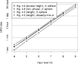
(a) Running times

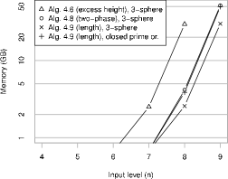
(b) Memory use

Figure 14: Performance of algorithms from Section 4

Figure 14 plots the actual running time and memory consumption from each of the calculations carried out in Sections 4.2 and 4.3. To recap, these calculations were:

• bounding excess heights by running the original Algorithm 4.6 and the two-phase Algorithm 4.8 over all 3-sphere triangulations of size $n$;

• bounding path lengths by running Algorithm 4.9 over all 3-sphere triangulations of size $n$, and over all size $n$ triangulations of closed prime orientable 3-manifolds.

Both plots use a log scale for the vertical axis. We omit $n=3$ (where time was negligible) and do not show memory under 1 GB (where overheads dominate). All computations were run on an 8-core 2.93 GHz Intel Xeon X5570 CPU with 72 GB of RAM. Algorithm 4.6 only shows $n\leq 8$, since the case $n=9$ required too much memory to run (recall that this was why we developed the two-phase Algorithm 4.8 to replace it). The data points for Algorithm 4.9 on closed prime orientable 3-manifolds represent sums taken over all such manifolds.

We can parallelise each of these algorithms by processing nodes simultaneously: for Algorithms 4.6 and 4.8 we simultaneously process nodes at the same level of the subgraph $G$, and for Algorithm 4.9 we simultaneously process nodes at the same distance from the source set $S$. However, we must be careful to serialise any updates to global structures (these include the subgraph $G$ and union-find structures in Algorithms 4.6 and 4.8, and the queue of nodes to be processed in Algorithm 4.9). Because these global structures can grow super-exponentially large, we use a shared memory model on a single multi-core machine, and avoid distributed processing.

Figure 14(a) shows the total CPU time summed over all threads of execution. When parallelised over all eight cores, the wall time was close to $1/8$ of these figures—for instance, the peak 46.6 days of CPU time for Algorithm 4.9 (closed prime orientable 3-manifolds, $n=9$) represented just 5.9 days of wall time. Despite the serialisation bottlenecks, all three algorithms achieved over $98\%$ CPU utilisation for the largest cases. This indicates that the task of identifying and following arcs in the Pachner graphs (which could be parallelised) was significantly more expensive than querying and updating the global structures (which could not).

For connecting minimal triangulations, Algorithms 4.12 and 4.14 are cheap in comparison: these required just 2.5 and 6.2 minutes of CPU time respectively to process the entire census of minimal triangulations, and each used under 1 GB of memory.

5 Pathological cases

In this section we first examine the most difficult triangulation to simplify from our tables, and we show how this pathological case corresponds to the “exceptional” brick $B_{5}$ in the Martelli-Petronio census [23]. Following this, we construct larger triangulations of graph manifolds that show how our excess height results do not generalise for arbitrary closed prime orientable 3-manifolds. In Section 6 we return to the important case of the 3-sphere, where no such counterexamples are known.

In the discussions below we use alphanumeric isomorphism signatures to identify specific 3-manifold triangulations. The appendix of this paper includes a full specification detailing how such signatures encode tables of tetrahedron face gluings. Alternatively, the software package Regina [10] can be used to “decode” these signatures back into 3-manifold triangulations.

5.1 Triangulations requiring many moves

Recall Theorem 4.3, where we show that one-vertex triangulations of closed prime orientable 3-manifolds of size $n\leq 9$ can be simplified using at most 17 Pachner moves. Although this bound is tight if we allow at most two extra tetrahedra (Lemma 4.10), the worst case is extremely rare: just one of the $50\,778\,377$ triangulations in Table 5 requires all 17 moves. We denote this worst-case triangulation by $\mathcal{T}_{\mathrm{max}}$. This triangulation is an outlier (the next-worst cases require just 13 moves), and we examine it here in detail.

$\mathcal{T}_{\mathrm{max}}$ has isomorphism signature jLAMLLQbcbdeghhiixxnxxjqisj, contains $n=9$ tetrahedra, and represents a Seifert fibred space over the 2-sphere with three exceptional fibres; specifically, $\mathrm{SFS}\left(S^{2}:(2,1)\ (3,1)\ (11,-9)\right)$. It has the structure of an augmented triangular solid torus, a common construction for Seifert fibred spaces [1, 27]: we build a 3-tetrahedron triangular prism, glue the triangular ends together, and attach either a layered solid torus or a Möbius band to each rectangular face. Figure 15 outlines the construction; see [1] for full details and notation.

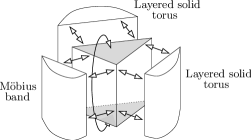
Figure 15: Building the augmented triangular solid torus $\mathcal{T}_{\mathrm{max}}$

This Seifert fibred space has only one minimal triangulation, with $n=8$ tetrahedra and isomorphism signature iLLLPQcbcgffghhhtsmhgosof. We denote this by $\mathcal{T}_{\mathrm{min}}$. Unlike $\mathcal{T}_{\mathrm{max}}$, the 8-tetrahedron $\mathcal{T}_{\mathrm{min}}$ is constructed not from prisms and layerings, but from the brick $B_{5}$ described by Martelli and Petronio in their census paper [23]. This brick $B_{5}$ is an 8-tetrahedron triangulation of the bounded Seifert fibred space $\mathrm{SFS}\left(D:(2,1)\ (3,1)\right)$, where $D$ denotes the 2-dimensional disc, and the three boundary edges of $B_{5}$ describe relatively complex curves on its torus boundary.

The brick $B_{5}$ is unique in the Martelli-Petronio census in that it is the only large brick that allows Seifert fibred spaces to be built using fewer tetrahedra than standard prism-and-layering constructions. However, it only appears rarely in the census; this is due to the specific parameters $\mathrm{SFS}\left(D:(2,1)\ (3,1)\right)$, the complex boundary curves, and the large number of tetrahedra. Indeed, amongst all minimal triangulations of closed prime orientable 3-manifolds of size $\leq 8$, the triangulation $\mathcal{T}_{\mathrm{min}}$ is the only one to contain $B_{5}$ at all.

In a sense then, the 17 moves needed to simplify $\mathcal{T}_{\mathrm{max}}$ indicate that $B_{5}$ is “substantially different” from standard prism-and-layering constructions: because $\mathcal{T}_{\mathrm{min}}$ is the only smaller triangulation of the same manifold, we are forced to reorganise the tetrahedra of $\mathcal{T}_{\mathrm{max}}$ to form a $B_{5}$ configuration in order to simplify it.

It is tempting to use $B_{5}$ to search for larger triangulations that require even more moves to simplify, but initial attempts are unsuccessful. Stepping up to nine tetrahedra, there are three minimal triangulations of closed prime orientable 3-manifolds that include the brick $B_{5}$: these represent the spaces $\mathrm{SFS}\left(S^{2}:(2,1)\ (3,1)\ (13,-11)\right)$, $\mathrm{SFS}\left(S^{2}:(2,1)\ (3,1)\ (16,-13)\right)$ and $\mathrm{SFS}\left(S^{2}:(2,1)\ (3,1)\ (17,-14)\right)$. The corresponding augmented triangular solid tori each have $n=10$ tetrahedra, and a computer search shows that each can be simplified using 17 Pachner moves once again.

5.2 Triangulations requiring greater excess height

In Theorems 4.2 and 4.4, we show that one-vertex triangulations of closed prime orientable 3-manifolds of size $n\leq 9$ can be simplified using at most two extra tetrahedra, and that any two minimal triangulations of such a manifold can be connected using at most two extra tetrahedra. Here we show that for arbitrary manifolds, these results do not generalise: in particular, we construct triangulations of graph manifolds with $n=10$ tetrahedra for which three extra tetrahedra are required.

All of the graph manifolds described in this section are obtained by joining two bounded Seifert fibred spaces along their torus boundaries according to a given $2\times 2$ matching matrix. We refer the reader to [4] for further details and notation.

Theorem 5.1.

There exists a closed prime orientable 3-manifold $\mathcal{M}$ and a node $\nu\in\mathscr{P}_{1}(\mathcal{M})$ at level $>\beta_{1}(\mathcal{M})$ from which every simplification path has excess height $\geq 3$.

Proof.

Let $\mathcal{M}$ be the graph manifold $\mathrm{SFS}\left(D:(2,1)\ (3,1)\right)\ \cup/{\mbox{\tiny $\!\left[\begin{array}[]{@{\ }r@{\ }r@{\ }}-1&1\\ 1&0\end{array}\right]$ }}\ \mathrm{SFS}\left(D:(3,2)\ (3,2)\right)$. The census of minimal triangulations in [4] shows that $\mathcal{M}$ has just one minimal triangulation; this has $\beta_{1}(\mathcal{M})=9$ tetrahedra and isomorphism signature jLLALPQaceefgihhijkuxpwhwns.

Let $\nu$ be the node of $\mathscr{P}_{1}(\mathcal{M})$ that describes the triangulation with size $n=10$ and isomorphism signature kLLzLQAkaceiggghijjjkxuaatlsqw. A computer search shows that no path from $\nu$ with excess height $\leq 2$ can reach level 9 of $\mathscr{P}_{1}(\mathcal{M})$. However, with excess height 3 we obtain a simplification path that connects $\nu$ with the unique minimal triangulation described above. ∎

The example above was found as a side-effect of processing the 10-tetrahedron census of minimal triangulations [4]: it was difficult to identify which manifold the triangulation represented, and this was only resolved after (with some difficulty) converting it into a known triangulation of the graph manifold $\mathcal{M}$. No other pathological cases have been found in this way. The 10-tetrahedron triangulation above is not based on a standard prism-and-layering construction, although the 9-tetrahedron minimal triangulation of $\mathcal{M}$ is.

Theorem 5.2.

There exists a closed prime orientable 3-manifold $\mathcal{M}$ and nodes $\nu_{1},\nu_{2}\in\mathscr{P}_{1}(\mathcal{M})$ at level $\beta_{1}(\mathcal{M})$ for which every path that joins $\nu_{1}$ with $\nu_{2}$ has excess height $\geq 3$.

Proof.

Recall that, unlike the census of all triangulations of closed prime orientable 3-manifolds, the census of all minimal triangulations of such manifolds extends to 11 tetrahedra [8]. By running Algorithm 4.12 over this extended census, we identify seven manifolds $\mathcal{M}$ for which $H_{\mathrm{min}}(\mathcal{M})=3$ (and none for which $H_{\mathrm{min}}(\mathcal{M})>3$). By Lemma 4.13, it follows that each of the corresponding Pachner graphs $\mathscr{P}_{1}(\mathcal{M})$ has nodes $\nu_{1},\nu_{2}$ with the property above. Table 9 summarises these results. ∎

Level	Manifold $\mathcal{M}$	Nodes at	Bound
$\beta_{1}(\mathcal{M})$		level $\beta_{1}(\mathcal{M})$	$H_{\mathrm{min}}(\mathcal{M})$
10	$\mathrm{SFS}\left(D:(2,1)\ (3,1)\right)\ \cup/{\mbox{\tiny $\!\left[\begin{array}[]{@{\ }r@{\ }r@{\ }}1&-1\\ 0&1\end{array}\right]$ }}\ \mathrm{SFS}\left(D:(3,2)\ (3,2)\right)$	6	3
11	$\mathrm{SFS}\left(D:(2,1)\ (3,1)\right)\ \cup/{\mbox{\tiny $\!\left[\begin{array}[]{@{\ }r@{\ }r@{\ }}-1&1\\ 1&-2\end{array}\right]$ }}\ \mathrm{SFS}\left(D:(3,2)\ (3,2)\right)$	18	3
11	$\mathrm{SFS}\left(D:(2,1)\ (3,1)\right)\ \cup/{\mbox{\tiny $\!\left[\begin{array}[]{@{\ }r@{\ }r@{\ }}1&-1\\ 0&1\end{array}\right]$ }}\ \mathrm{SFS}\left(D:(3,2)\ (4,1)\right)$	9	3
11	$\mathrm{SFS}\left(D:(2,1)\ (3,1)\right)\ \cup/{\mbox{\tiny $\!\left[\begin{array}[]{@{\ }r@{\ }r@{\ }}1&-1\\ 0&1\end{array}\right]$ }}\ \mathrm{SFS}\left(D:(3,2)\ (4,3)\right)$	9	3
11	$\mathrm{SFS}\left(D:(2,1)\ (3,1)\right)\ \cup/{\mbox{\tiny $\!\left[\begin{array}[]{@{\ }r@{\ }r@{\ }}1&-1\\ 0&1\end{array}\right]$ }}\ \mathrm{SFS}\left(D:(3,2)\ (5,2)\right)$	9	3
11	$\mathrm{SFS}\left(D:(2,1)\ (3,1)\right)\ \cup/{\mbox{\tiny $\!\left[\begin{array}[]{@{\ }r@{\ }r@{\ }}1&-1\\ 0&1\end{array}\right]$ }}\ \mathrm{SFS}\left(D:(3,2)\ (5,3)\right)$	9	3
11	$\mathrm{SFS}\left(D:(2,1)\ (4,1)\right)\ \cup/{\mbox{\tiny $\!\left[\begin{array}[]{@{\ }r@{\ }r@{\ }}1&-1\\ 0&1\end{array}\right]$ }}\ \mathrm{SFS}\left(D:(3,2)\ (3,2)\right)$	6	3

Table 9: Manifolds from the 11-tetrahedron census with $H_{\mathrm{min}}(\mathcal{M})>2$

As with Theorem 5.1, all of the manifolds in Table 9 are graph manifolds. We return to this issue in Section 6, where we discuss the lack of known pathological examples for “simple” manifolds (in particular, the 3-sphere).

6 Discussion

As noted already, the bounds on simplification paths that we obtain in Section 4 are astonishingly small. Although we only consider triangulations of size $n\leq 9$, this is not a small sample: the census includes $\sim 150$ million triangulations, including $\sim 31$ million one-vertex 3-spheres, plus another $\sim 51$ million one-vertex triangulations of $1\,900$ distinct closed prime orientable 3-manifolds that cover all eight Thurston geometries as well as non-geometric combinations of these [24].

These results have interesting implications for simplification algorithms. Given a triangulation $\mathcal{T}$ (of arbitrary size) that we wish to simplify, we can follow the strategy of Algorithm 4.9 and perform a breadth-first search from $\mathcal{T}$ using Pachner moves and octahedron, pillow and prism flips, never adding more than two extra tetrahedra. Theorem 4.2 gives us hope that this will indeed simplify $\mathcal{T}$, and Theorem 4.3 gives us hope that the search will be relatively fast. Initial observations from using such simplification techniques in ongoing research projects show them to be remarkably successful.

Triangulations of the 3-sphere exhibit particularly good behaviour. In contrast to closed prime orientable manifolds, the worst-case number of moves needed to simplify a 3-sphere triangulation barely grows at all with the size $n$ (Figure 13). Moreover, unlike the graph manifolds discussed in Section 5, there are no known pathological 3-sphere triangulations that require more than two extra tetrahedra to simplify, despite the 3-sphere having far more triangulations than any other manifold in the census. These results lead us to make the following conjecture:

Conjecture 6.1.

From any node at any level $n\geq 3$ of the graph $\mathscr{P}_{1}(S^{3})$, there is a simplification path of excess height $\leq 2$.

If true, this would help explain why 3-sphere triangulations are so easy to simplify in practice. Moreover, by combining this result with Theorem 3.1, we could reduce Mijatović’s bound on the number of Pachner moves needed to simplify a one-vertex triangulation of the 3-sphere from $\exp(O(n^{2}))$ down to $\exp(O(n\log n))$ instead.

There are theoretical reasons to believe that Conjecture 6.1 might be true. Similar results are known for the simplification of knots in $\mathbb{R}^{3}$: Dynnikov shows that an arc presentation of the trivial knot can be simplified using elementary moves without increasing the complexity of the diagram [13, 14], and Henrich and Kauffman use his results to show that any projection of the unknot can be simplified using Reidemeister moves with only a quadratic increase in the number of crossings [16]. In the setting of triangulation simplification, Mijatović’s bounds for the 3-sphere—though extremely large—remain far smaller than for other manifolds (whose bounds involve towers of exponentials). Moreover, every pathological triangulation from Section 5 that requires three extra tetrahedra is of a non-geometric graph manifold: it is possible that the boundaries between geometric components in such manifolds act as barriers to simplification that would not exist for the 3-sphere.

We now turn our attention to path length; that is, the number of Pachner moves required to simplify a triangulation. Our next conjecture involves the average simplification path lengths $\sigma_{n}$ (for 3-sphere triangulations) and $\pi_{n}$ (for closed prime orientable 3-manifold triangulations), as defined in Section 4.3.

Conjecture 6.2.

Both quantities $\sigma_{n}$ and $\pi_{n}$ are in $O(1)$; that is, they are bounded above by a constant that does not depend on $n$.

This conjecture is clearly supported by the results in Figure 13. Looking more closely at Tables 4 and 5 however, we can formulate a more interesting observation:

Conjecture 6.3.

For a given 3-manifold $\mathcal{M}$, let $\phi_{n}(\mathcal{M})$ denote the fraction of nodes at level $n$ of $\mathscr{P}_{1}(\mathcal{M})$ that have an arc leading directly down to level $n-1$. Then, if $\mathcal{M}$ is the 3-sphere or a closed prime orientable 3-manifold, $\lim_{n\to\infty}\phi_{n}(\mathcal{M})=1$.

In other words, as $n\to\infty$, almost all size $n$ triangulations of the 3-sphere or of closed prime orientable 3-manifolds can be simplified immediately, using just a single 3-2 move. Intuitively this seems reasonable, since with more tetrahedra it is more likely that a suitable degree three edge can be found. However, proving it appears difficult: like most probabilistic arguments involving 3-manifold triangulations, we run into the critical problem that almost all pairwise gluings of tetrahedron faces do not represent 3-manifolds at all [12].

This observation can be framed in terms of generic complexity [33], where we are allowed to ignore a vanishingly small population of pathological inputs. In this context, Conjecture 6.3 states that generic triangulations of $S^{3}$ or of closed prime orientable 3-manifolds can be simplified in a single move. An interesting direction for future research is to build a 3-sphere recognition algorithm based on Pachner moves that runs in polynomial time for generic inputs.

We return now to worst case path length for 3-sphere triangulations. Again, we observe from Figure 13 that the worst-case bound $L_{n}(S^{3})$ barely changes at all for $3\leq n\leq 9$: there is just one increment, which is of the smallest possible size (recalling that $L_{n}$ must always be odd). This is in contrast to the case of arbitrary closed prime orientable manifolds, where the worst-case path length grows with $n$, and does so at a clearly accelerating rate.

This slow rate of growth for $L_{n}(S^{3})$ has direct implications for the complexity of 3-sphere recognition:

Observation 6.4.

If $L_{n}(S^{3})\in o(n/\log n)$, then there is a 3-sphere recognition algorithm with running time in $o(\alpha^{n})$ for any $\alpha>1$. That is, the 3-sphere can be recognised in sub-exponential time.

Proof.

From any $n$-tetrahedron triangulation $\mathcal{T}$ there are at most $O(n)$ possible 2-3 or 3-2 moves (one for each face or edge of $\mathcal{T}$). We can therefore enumerate all possible sequences of $k$ moves in $O\left(n^{t}\cdot(n+k)^{k}\right)$ time, where $n^{t}$ is a small polynomial term that accounts for the mechanics of performing each 2-3 or 3-2 move. Setting $k=L_{n}(S^{3})$ and observing that $n+k\in O(n)$, we find that if $\mathcal{T}$ can be simplified, this can be done in $O\left(n^{t+L_{n}(S^{3})}\right)$ time.

Repeating this operation $n-2$ times, we can either simplify $\mathcal{T}$ to a known 2-tetrahedron triangulation of $S^{3}$, or else show this to be impossible. The total running time is

$$O\left(n\cdot n^{t+L_{n}(S^{3})}\right)=O\left(n^{t+1}\cdot\exp\left(\log n\cdot L_{n}(S^{3})\right)\right).$$

Since $L_{n}(S^{3})\in o(n/\log n)$, this running time is $o(\alpha^{n})$ for any $\alpha>1$. ∎

Although there is too little data to predict the precise growth rate of $L_{n}(S^{3})$ (a situation that Theorem 3.1 shows is extremely difficult to rectify), it is certainly plausible to suggest from Figure 13 that $L_{n}(S^{3})$ is “sufficiently sublinear” to satisfy $L_{n}(S^{3})\in o(n/\log n)$. This leads us to the following conjecture:

Conjecture 6.5.

From any node at any level $n\geq 3$ of the graph $\mathscr{P}_{1}(S^{3})$, there is a simplification path of length $\leq L_{n}(S^{3})$ where $L_{n}(S^{3})\in o(n/\log n)$, and therefore sub-exponential time 3-sphere recognition is possible.

If this conjecture could be proven, the resulting sub-exponential time 3-sphere recognition algorithm would be a significant breakthrough in algorithmic 3-manifold topology.

Appendix: Isomorphism signatures

In Section 3.2 we describe isomorphism signatures, which are small pieces of data that uniquely define the isomorphism class of a triangulation, and that can be computed in small polynomial time. Recall that to compute an isomorphism signature, we must:

1. enumerate all $O(n)$ canonical labellings of the input triangulation;

2. encode the full set of face gluings for each canonical labelling;

3. choose the lexicographically smallest encoding amongst all canonical labellings.

In this appendix we specify the encoding used in step (ii). For the theoretical arguments in Section 3.2, it is sufficient to use a simple bit sequence that encodes the complete table of face gluings. In practice however, we use a more compact method:

• we do not encode redundant information from the face gluings table;

• we use printable characters (letters, digits and punctuation) instead of plain bits.

In this way, the encoding is kept short but remains easy to write or type by hand. This is useful in both papers and software: authors can describe triangulations precisely without presenting large tables of face gluings (as seen in Section 5 of this paper), and readers can reconstruct these triangulations quickly using the appropriate software.

The precise encoding described here is implemented in version 4.90 of the freely-available software package Regina [10]. This encoding method is defined not only for closed triangulations (as described in this paper), but also for triangulations with boundary (where some tetrahedron faces are not glued to any partner face) and ideal triangulations (where some vertex neighbourhoods are not bounded by spheres). The encoding draws upon and extends ideas from the dehydration format of Callahan et al. [11].

Encoding integers

A key piece of the encoding process is to translate integers into printable characters. We describe two methods: one for “small” integers in the range $0,\ldots,63$, and one for “large” integers in the range $0,\ldots,n$.

For small integers, we use the following translation table from $0,\ldots,63$ to printable characters. This is similar to, but not the same as, a typical Base64 encoding table. For each $i\in\{0,\ldots,63\}$ we let $\pi(i)$ denote the corresponding printable character.

$$\begin{array}[]{l|ccc|ccc|ccc|c|c}\mbox{Integer $i$}&0&\cdots&25&26&\cdots&51&52&\cdots&61&62&63\\ \hline\cr\mbox{Printable character $\pi(i)$}&\mathtt{a}&\cdots&\mathtt{z}&\mathtt{A}&\cdots&\mathtt{Z}&\mathtt{0}&\cdots&\mathtt{9}&\mathtt{+}&\mathtt{-}\end{array}$$

To encode large integers we use $d$ printable characters, where $d=\lfloor\log_{64}(n)\rfloor+1$. Specifically: for any integer $i\in\{0,\ldots,n\}$, we write $i$ as a $d$-digit number in base 64, and then use $\pi(\cdot)$ to encode the individual digits as described above, beginning with the least significant digit. We denote the resulting string of characters by $\epsilon(i)$.

For example, suppose that $n=100$ and we wish to encode the integer $i=93$. This encoding uses $d=\lfloor\log_{64}(100)\rfloor+1=2$ characters. Since $93=29+1\cdot 64$, the two base 64 “digits” of $i$ are $(29,1)$. The final encoding is then $\epsilon(93)=\pi(29)\pi(1)=\mathtt{Db}$.

If $i\ll n$, we may need to pad the base 64 representation of $i$ with leading zeroes. For instance, if $n=100$ and we wish to encode $i=5$, the two base 64 “digits” are $(5,0)$, and the final encoding is $\epsilon(5)=\pi(5)\pi(0)=\mathtt{fa}$.

Encoding face gluings

Here we identify the information required to reconstruct the full table of face gluings for a canonical labelling. Such a table can be seen in Table 2 (from Section 3.2), which we use as an example throughout this discussion.

We begin by removing redundant information from the gluings table. Suppose that face $f$ of tetrahedron $t$ is glued to face $f^{\prime}$ of tetrahedron $t^{\prime}$. If $(t^{\prime},f^{\prime})<(t,f)$ lexicographically, then we delete the table cell in position $(t,f)$. This is because the same gluing has already been seen from the other direction in cell $(t^{\prime},f^{\prime})$, and so the information in cell $(t,f)$ is redundant. Table 10 shows a copy of Table 2 with these redundant cells crossed out.

	Face 0	Face 1	Face 2	Face 3
	Vertices 123	Vertices 023	Vertices 013	Vertices 012
Tet. 0	Tet. 0:   120	Tet. 1:   023	Tet. 2:   013	Tet. 0:   312
Tet. 1	Tet. 2:   230	Tet. 0:   023	Tet. 1:   012	Tet. 1:   013
Tet. 2	Tet. 2:   012	Tet. 1:   312	Tet. 0:   013	Tet. 2:   123

Table 10: Removing redundant information from the face gluings table

To reconstruct the table cells that remain, we extract the following information:

• Destination sequence: As in Section 3.2, let $A_{t,f}$ denote the tetrahedron glued to face $f$ of tetrahedron $t$, so that $A_{t,f}\in\{\partial,0,\ldots,n-1\}$ for all $t=0,\ldots,n-1$ and $f=0,\ldots,3$. Here we use the special symbol $A_{t,f}=\partial$ to indicate that face $f$ of tetrahedron $t$ is a boundary face, i.e., it is not glued to any partner tetrahedron face at all. The destination sequence is obtained by writing out $A_{0,0},A_{0,1},A_{0,2},A_{0,3},\allowbreak A_{1,0},\ldots,A_{n-1,3}$, and then deleting any entries $A_{t,f}$ that correspond to deleted table cells $(t,f)$.

  For our example in Table 10, the corresponding destination sequence is $0,1,2,2,1,2$.

• Type sequence: For each term $A_{t,f}$ in the destination sequence, we classify the corresponding tetrahedron face as one of the following three types:

  • Type 0: This indicates that the face is a boundary face, i.e., $A_{t,f}=\partial$.

  • Type 1: This indicates that the face is joined to a new tetrahedron. That is, $A_{t,f}=k$ where (i) $k\geq 1$, and (ii) the term $A_{t,f}$ is the first time that $k$ appears in the destination sequence.

  • Type 2: This indicates that the face is joined to an old tetrahedron. That is, either $A_{t,f}=0$, or else $A_{t,f}=k\geq 1$ but there is some other term $A_{t^{\prime},f^{\prime}}=k$ that appears in the destination sequence earlier than $A_{t,f}$.

  We obtain the type sequence by writing out the corresponding face type for each term in the destination sequence.

  For our example, the type sequence is $2,1,1,2,2,2$. The two ‘1’s in this sequence correspond to the first appearances of tetrahedra 1 and 2, in cells $(0,1)$ and $(0,2)$ respectively of the face gluings table.

• Permutation sequence: For each non-boundary tetrahedron face $(t,f)$ that is glued to some partner face $(t^{\prime},f^{\prime})$, we identify the corresponding gluing permutation $p_{t,f}\in S_{4}$. This is the permutation for which $p_{t,f}(f)=f^{\prime}$, and each vertex $v\neq f$ of tetrahedron $t$ maps to vertex $p_{t,f}(v)\neq f^{\prime}$ of tetrahedron $t^{\prime}$ under this face gluing.

  We can represent each permutation in $S_{4}$ by a number: simply order them lexicographically and number them $0,\ldots,23$. The identity $(0,1,2,3)\mapsto(0,1,2,3)$ becomes 0, the permutation $(0,1,2,3)\mapsto(0,1,3,2)$ becomes 1, and so on until $(0,1,2,3)\mapsto(3,2,1,0)$ becomes 23.

  To build the permutation sequence, we write out the number for each permutation $p_{t,f}$ corresponding to each term $A_{t,f}\neq\partial$ in the destination sequence.

  In our example, this sequence is $21,0,0,9,1,18$. The two ‘0’s come from the faces of type 1: because the labelling is canonical, those permutations must be the identity.

The full isomorphism signature

To completely encode a labelled triangulation, we bundle all of the above information into a sequence of printable characters as follows.

• We begin the sequence by encoding $n$ and $d$ (recall that $d$ indicates how many printable characters are required to encode each “large integer” in the range $0,\ldots,n$). Specifically: if $n\geq 63$ then we begin with the special marker $\pi(63)$ followed by $\pi(d)$ and $\epsilon(n)$. If $n<63$, we simply begin with $\pi(n)$ and it is implicitly understood that $d=1$.

  Strictly speaking, because we encode $\pi(d)$, this scheme only works if $d<64$. However, this is true for all $n<64^{63}\simeq 6\times 10^{113}$, which covers all conceivable practical requirements.

• We follow this with the type sequence. Since each face type is in $\{0,1,2\}$, we can encode three terms of the sequence in each printable character. Specifically, if the type sequence is $t_{0},t_{1},\ldots$, then we write $\pi(t_{0}+4t_{1}+16t_{2})$, $\pi(t_{3}+4t_{4}+16t_{5})$, …, padding the sequence with one or two trailing zeroes if necessary.

• Next we write the destination sequence, but only for faces of type 2. Each destination $A_{t,f}$ is encoded as $\epsilon(A_{t,f})$. We ignore the other faces because type 0 faces are boundary, and type 1 destinations can be deduced from the fact that the labelling is canonical.

• We finish with the permutation sequence, again only for faces of type 2. Each permutation number $i$ is encoded as $\pi(i)$. We ignore type 1 faces because, in a canonical labelling, all type 1 gluings must use the identity permutation.

For our example: since $n=3<63$, we begin the sequence with $\pi(3)=\mathtt{d}$. The type sequence $2,1,1,2,2,2$ encodes to $\pi(2+1\cdot 4+1\cdot 16)$ followed by $\pi(2+2\cdot 4+2\cdot 16)$; that is, $\pi(22)\pi(42)=\mathtt{wQ}$. The destination sequence for type 2 faces is $0,2,1,2$, which encodes to $\mathtt{acbc}$. The permutation sequence for type 2 faces is $21,9,1,18$, which encodes to $\mathtt{vjbs}$. We combine these pieces to obtain the final sequence dwQacbcvjbs.

To obtain an isomorphism signature, we must choose the lexicographically smallest encoding amongst all canonical labellings. For this we order printable characters according to the standard ASCII tables (so, for instance, $\mathtt{1}<\mathtt{Z}<\mathtt{a}$). This keeps things simple for programmers, who can using ready-made comparison functions such as strcmp in C.

In our example, the encoding dwQacbcvjbs from Table 10 is not an isomorphism signature. Several different canonical labellings give lexicographically smaller encodings; the smallest is dLQabccbcjj, which becomes the isomorphism signature for this triangulation.

As a final remark, we can easily extend isomorphism signatures to support disconnected triangulations (which are not considered in this paper): simply list the signatures for each connected component in sorted order.

Benjamin A. Burton
School of Mathematics and Physics, The University of Queensland
Brisbane QLD 4072, Australia
(bab@maths.uq.edu.au)

References

- [1] Benjamin A. Burton, Minimal triangulations and normal surfaces, Ph.D. thesis, University of Melbourne, 2003, available from http://regina.sourceforge.net/.
- [2] , Face pairing graphs and 3-manifold enumeration, J. Knot Theory Ramifications 13 (2004), no. 8, 1057–1101.
- [3] , Introducing Regina, the 3-manifold topology software, Experiment. Math. 13 (2004), no. 3, 267–272.
- [4] , Enumeration of non-orientable 3-manifolds using face-pairing graphs and union-find, Discrete Comput. Geom. 38 (2007), no. 3, 527–571.
- [5] , The complexity of the normal surface solution space, SCG ’10: Proceedings of the Twenty-Sixth Annual Symposium on Computational Geometry, ACM, 2010, pp. 201–209.
- [6] , Optimizing the double description method for normal surface enumeration, Math. Comp. 79 (2010), no. 269, 453–484.
- [7] , Quadrilateral-octagon coordinates for almost normal surfaces, Experiment. Math. 19 (2010), no. 3, 285–315.
- [8] , Detecting genus in vertex links for the fast enumeration of 3-manifold triangulations, ISSAC 2011: Proceedings of the 36th International Symposium on Symbolic and Algebraic Computation, ACM, 2011, pp. 59–66.
- [9] , The Pachner graph and the simplification of 3-sphere triangulations, SCG ’11: Proceedings of the Twenty-Seventh Annual Symposium on Computational Geometry, ACM, 2011, pp. 153–162.
- [10] Benjamin A. Burton, Ryan Budney, William Pettersson, et al., Regina: Software for 3-manifold topology and normal surface theory, http://regina.sourceforge.net/, 1999–2011.
- [11] Patrick J. Callahan, Martin V. Hildebrand, and Jeffrey R. Weeks, A census of cusped hyperbolic 3-manifolds, Math. Comp. 68 (1999), no. 225, 321–332.
- [12] Nathan M. Dunfield and William P. Thurston, Finite covers of random 3-manifolds, Invent. Math. 166 (2006), no. 3, 457–521.
- [13] I. A. Dynnikov, Recognition algorithms in knot theory, Uspekhi Mat. Nauk 58 (2003), no. 6(354), 45–92.
- [14] , Arc-presentations of links: Monotonic simplification, Fund. Math. 190 (2006), 29–76.
- [15] Masao Hara, Seiichi Tani, and Makoto Yamamoto, is in , SODA ’05: Proceedings of the Sixteenth Annual ACM-SIAM Symposium on Discrete Algorithms, Society for Industrial and Applied Mathematics, 2005, pp. 359–364.
- [16] A. Henrich and L. Kauffman, Upper bounds for an unknotting sequence of Reidemeister moves, Preprint, arXiv:1006.4176v3, April 2011.
- [17] William Jaco, David Letscher, and J. Hyam Rubinstein, Algorithms for essential surfaces in 3-manifolds, Topology and Geometry: Commemorating SISTAG, Contemporary Mathematics, no. 314, Amer. Math. Soc., Providence, RI, 2002, pp. 107–124.
- [18] William Jaco and J. Hyam Rubinstein, 0-efficient triangulations of 3-manifolds, J. Differential Geom. 65 (2003), no. 1, 61–168.
- [19] , Layered-triangulations of 3-manifolds, Preprint, arXiv:math/0603601, March 2006.
- [20] William Jaco and Jeffrey L. Tollefson, Algorithms for the complete decomposition of a closed -manifold, Illinois J. Math. 39 (1995), no. 3, 358–406.
- [21] Bruce Kleiner and John Lott, Notes on Perelman’s papers, Geom. Topol. 12 (2008), no. 5, 2587–2855.
- [22] Bruno Martelli, Complexity of 3-manifolds, Spaces of Kleinian Groups, London Math. Soc. Lecture Note Ser., vol. 329, Cambridge Univ. Press, Cambridge, 2006, pp. 91–120.
- [23] Bruno Martelli and Carlo Petronio, Three-manifolds having complexity at most 9, Experiment. Math. 10 (2001), no. 2, 207–236.
- [24] Sergei Matveev, Algorithmic topology and classification of 3-manifolds, Algorithms and Computation in Mathematics, no. 9, Springer, Berlin, 2003.
- [25] Sergei V. Matveev, Complexity theory of three-dimensional manifolds, Acta Appl. Math. 19 (1990), no. 2, 101–130.
- [26] , Computer recognition of three-manifolds, Experiment. Math. 7 (1998), no. 2, 153–161.
- [27] , Tables of 3-manifolds up to complexity 6, Max-Planck-Institut für Mathematik Preprint Series (1998), no. 67, available from http://www.mpim-bonn.mpg.de/html/preprints/preprints.html.
- [28] , Tabulation of three-dimensional manifolds, Russian Math. Surveys 60 (2005), no. 4, 673–698.
- [29] Aleksandar Mijatović, Simplifying triangulations of , Pacific J. Math. 208 (2003), no. 2, 291–324.
- [30] , Triangulations of Seifert fibred manifolds, Math. Ann. 330 (2004), no. 2, 235–273.
- [31] , Simplical structures of knot complements, Math. Res. Lett. 12 (2005), no. 5-6, 843–856.
- [32] , Triangulations of fibre-free Haken 3-manifolds, Pacific J. Math. 219 (2005), no. 1, 139–186.
- [33] Alexei Myasnikov, Vladimir Shpilrain, and Alexander Ushakov, Group-based cryptography, Advanced Courses in Mathematics. CRM Barcelona, Birkhäuser Verlag, Basel, 2008.
- [34] Udo Pachner, P.L. homeomorphic manifolds are equivalent by elementary shellings, European J. Combin. 12 (1991), no. 2, 129–145.
- [35] J. Hyam Rubinstein, An algorithm to recognize the -sphere, Proceedings of the International Congress of Mathematicians (Zürich, 1994), vol. 1, Birkhäuser, 1995, pp. 601–611.
- [36] Abigail Thompson, Thin position and the recognition problem for , Math. Res. Lett. 1 (1994), no. 5, 613–630.