Adaptive estimation of the conditional cumulative distribution function from current status data

Sandra Plancade sandra.c.plancade@uit.no Institute of Community Medicine, University of Tromso, 9037 Tromso, Norway
Abstract

Consider a positive random variable of interest Y𝑌Y depending on a covariate X𝑋X, and a random observation time T𝑇T independent of Y𝑌Y given X𝑋X. Assume that the only knowledge available about Y𝑌Y is its current status at time T𝑇T: δ=1I{YT}𝛿1subscriptI𝑌𝑇\delta=1\!\mbox{I}_{\{Y\leq T\}} with 1I1I1\!\mbox{I} the indicator function. This paper presents a procedure to estimate the conditional cumulative distribution function F𝐹F of Y𝑌Y given X𝑋X from an independent identically distributed sample of (X,T,δ)𝑋𝑇𝛿(X,T,\delta).

A collection of finite-dimensional linear subsets of L2(2)superscript𝐿2superscript2L^{2}(\mathbb{R}^{2}) called models are built as tensor products of classical approximation spaces of L2()superscript𝐿2L^{2}(\mathbb{R}). Then a collection of estimators of F𝐹F is constructed by minimization of a regression-type contrast on each model and a data driven procedure allows to choose an estimator among the collection. We show that the selected estimator converges as fast as the best estimator in the collection up to a multiplicative constant and is minimax over anisotropic Besov balls. Finally simulation results illustrate the performance of the estimation and underline parameters that impact the estimation accuracy.

keywords:
Current status , Interval Censoring , Distribution function , Model selection , Adaptivity , Anisotropic Besov spaces , Minimax.
journal: Journal of Statistical Planning and Inference

1 Introduction

Current status data framework refers to a situation where the observation of a positive variable of interest Y𝑌Y called lifetime, is restricted to the knowledge of whether or not Y𝑌Y exceeds a random measure time T𝑇T. More precisely, one only observes the time T𝑇T and the “current status” of the system at time T𝑇T, namely δ=1I{YT}𝛿1subscriptI𝑌𝑇\delta=1\!{\mbox{I}}_{\{Y\leq T\}} equal to 1 if YT𝑌𝑇Y\leq T and 0 otherwise. Such data arise naturally for example in infectious disease studies, when the time Y𝑌Y of infection is unobserved, and a test is carried out at time T𝑇T. This framework is also named interval censoring, case 1, since the observation (T,δ)𝑇𝛿(T,\delta) indicates whether Y𝑌Y lies in [0,T]0𝑇[0,T] or (T,+)𝑇(T,+\infty). Contrary to other censoring framework, such as the right-censoring, the variable of interest is never directly measured. Nevertheless, as the intervals [0,T]0𝑇[0,T] and (T,+)𝑇(T,+\infty) are different for each observation, quantities related to Y𝑌Y can be inferred.

The design considered in this paper is classical in current status data framework (e.g. Cheng and Wang (2011), van der Vaart and van der Laan (2006)): the survival and observation times Y𝑌Y and T𝑇T are assumed to be independent given a uni-dimensional covariate X𝑋X directly measured. In the first place, no smoothness conditions are assumed on the variables (X,Y,T)𝑋𝑌𝑇(X,Y,T). More precisely, the following i.i.d. sample is observed

(Xi,Ti,δi)i=1,,nsubscriptsubscript𝑋𝑖subscript𝑇𝑖subscript𝛿𝑖𝑖1𝑛(X_{i},T_{i},\delta_{i})_{i=1,\dots,n} (1)

with the survival times (Yi)i=1,,nsubscriptsubscript𝑌𝑖𝑖1𝑛(Y_{i})_{i=1,\dots,n} independent from the observation times (Ti)i=1,,nsubscriptsubscript𝑇𝑖𝑖1𝑛(T_{i})_{i=1,\dots,n} conditional to the covariates (Xi)i=1,,nsubscriptsubscript𝑋𝑖𝑖1𝑛(X_{i})_{i=1,\dots,n}, and (δi)i=1,,nsubscriptsubscript𝛿𝑖𝑖1𝑛(\delta_{i})_{i=1,\dots,n} denoting the indicators (1I{YiTi})i=1,,nsubscript1subscriptIsubscript𝑌𝑖subscript𝑇𝑖𝑖1𝑛(1\!{\mbox{I}}_{\{Y_{i}\leq T_{i}\}})_{i=1,\dots,n}. We aim to estimate the cumulative distribution function (c.d.f.) F𝐹F of Y𝑌Y given a covariate X𝑋X, namely

F(x,y)=P[Yy|X=x].𝐹𝑥𝑦𝑃delimited-[]𝑌conditional𝑦𝑋𝑥F(x,y)=P[Y\leq y|X=x].

Current status data have been widely studied over the past two decades. Most results about nonparametric estimation of the survival function are based on the NPMLE (Nonparametric Maximum Likelihood Estimator). Groeneboom and Wellner (1992) prove that the NPMLE is pointwise convergent with the optimal rate n1/3superscript𝑛13n^{-1/3}, and van de Geer (1993) establishes a similar result for the L2superscript𝐿2L^{2}-risk under the assumption of continuous survival time density. This unusual rate of convergence differs from the uncensored and right-censored designs, in which the distribution function can be estimated with the parametric rate of convergence n1/2superscript𝑛12n^{-1/2}.

More recently, estimators developed from the NPMLE take into account the regularity of the function. Hudgens et al. (2007) build three estimators derived from the NPMLE, and compare their performances on simulated and real data. van der Vaart and van der Laan (2006) apply smoothing methods to the NPLME to estimate the survival function in presence of high-dimensional covariates. Birgé (1999) proposes an easily computable histogram estimator which reaches the minimax rate of convergence. The procedures developed in these papers assume that the regularity of the target function is known.

Few papers propose estimators that automatically adapt to the unknown regularity of the function. Ma and Kosorok (2006) introduce a NPMLE and a least square estimator on Sobolev classes, and select the regularity parameter with a penalized criterion. Brunel and Comte (2009) draw a parallel between current status data and bounded regression framework through a least-square estimator combined with a model selection procedure based on a more easily computable penalty function. As far as the author knows, estimation of cumulative distribution function from current status data in presence of covariates has not been handled yet in an adaptive framework. Moreover, lower-bounds on classical regularity spaces are not available. This paper aims to address these two questions.

First of all, the procedure from Brunel and Comte (2009) is extended in order to include a covariate. For every i=1,,n𝑖1𝑛i=1,\dots,n,

𝔼[δi|Xi,Ti]=𝔼[1I{YiTi}|Xi,Ti]=[YiTi|Xi,Ti]=F(Xi,Ti).𝔼delimited-[]conditionalsubscript𝛿𝑖subscript𝑋𝑖subscript𝑇𝑖𝔼delimited-[]conditional1subscriptIsubscript𝑌𝑖subscript𝑇𝑖subscript𝑋𝑖subscript𝑇𝑖delimited-[]subscript𝑌𝑖conditionalsubscript𝑇𝑖subscript𝑋𝑖subscript𝑇𝑖𝐹subscript𝑋𝑖subscript𝑇𝑖\mathbb{E}[\delta_{i}|X_{i},T_{i}]=\mathbb{E}\left[1\!{\mbox{I}}_{\{Y_{i}\leq T_{i}\}}|X_{i},T_{i}\right]=\mathbb{P}[Y_{i}\leq T_{i}|X_{i},T_{i}]=F(X_{i},T_{i}).

Therefore, F𝐹F is the regression function of δisubscript𝛿𝑖\delta_{i} on (Xi,Ti)subscript𝑋𝑖subscript𝑇𝑖(X_{i},T_{i}) and a least-square contrast is considered. A collection of linear spaces of L2(×+)superscript𝐿2superscriptL^{2}(\mathbb{R}\times\mathbb{R}^{+}) is built by tensor product of classical approximation subspaces of L2()superscript𝐿2L^{2}(\mathbb{R}) and L2(+)superscript𝐿2superscriptL^{2}(\mathbb{R}^{+}). Finally, a model selection estimator is computed by penalization of the least-square contrast following the model selection procedure from Birgé and Massart (1998).

The loss function usually considered in model selection procedures is associated to the L2superscript𝐿2L^{2}-norm. Nevertheless, the least-square contrast which quantifies the goodness of fit on the observations provides a natural control of the risk associated to the empirical norm tn2=(1/n)i=1nt2(Xi,Ti)superscriptsubscriptnorm𝑡𝑛21𝑛superscriptsubscript𝑖1𝑛superscript𝑡2subscript𝑋𝑖subscript𝑇𝑖\|t\|_{n}^{2}=(1/n)\sum_{i=1}^{n}t^{2}(X_{i},T_{i}) which represents an intermediate result in the computation of the integrated risk in most model selection procedures (see e.g. Massart (2007), Comments of Theorem 8.3). In this paper, we have chosen to first display the control of the empirical risk conditional to the observations {(Xi,Ti)}subscript𝑋𝑖subscript𝑇𝑖\{(X_{i},T_{i})\} and then derive the result for the L2superscript𝐿2L^{2}-risk under additional assumptions in order to emphasize the role played by each hypothesis. Besides, the fixed design context with non-random observations {(Xi,Ti)}subscript𝑋𝑖subscript𝑇𝑖\{(X_{i},T_{i})\} can be directly handled.

On complementary interest to the adaptivity on decomposition bases, is the study of the rate of convergence on spaces of regularity. Anisotropic Besov spaces, which account for different regularities of the target function F𝐹F with respect to the covariate X𝑋X and the survival time Y𝑌Y, are considered. On the one hand, the rate of convergence of our adaptive estimator is evaluated, exhibiting classical rates in a regression context, but unusual in c.d.f. estimation. On the other hand, the minimax rate of convergence is considered as a criterion to evaluate the fundamental limit of the current status framework. The combination of these two analyses assesses the optimality of our estimator. Results in a context without covariate can be derived as a particular case, proving the optimality of the estimators proposed by Ma and Kosorok (2006) and Brunel and Comte (2009).

Furthermore, we analyze the performance of our estimator on simulated data. In a right-censoring context, the rate of censoring defined as the proportion of censored observations is a well-identified parameter of the quality of the estimation. Since the survival time is never observed in current status data, this quantity makes no sense. Nevertheless, in our numerical study, we exhibit a parameter which impacts the estimation from current status data, and may represent the counterpart of the rate of censoring on right-censored data.

The paper is organized as follows. Section 2 introduces the notations. The estimation procedure is presented in Section 3. The upper-bounds for the empirical and integrated loss functions are presented in Section 4. The minimax study over anisotropic Besov balls is conducted in Section 5. Section 6 displays the performances of the estimator on simulated data. General comments and perspectives for further developments are presented in Section 7. The proofs are gathered in Section 8.

2 Notations

2.1 Notations

Let X and T denote the vectors (X1,,Xn)subscript𝑋1subscript𝑋𝑛(X_{1},\dots,X_{n}) and (T1,,Tn)subscript𝑇1subscript𝑇𝑛(T_{1},\dots,T_{n}), and for every tL2(×+)𝑡superscript𝐿2superscriptt\in L^{2}(\mathbb{R}\times\mathbb{R}^{+}), let t(𝐗,𝐓)=(t(X1,T1),,t(Xn,Tn))𝑡𝐗𝐓𝑡subscript𝑋1subscript𝑇1𝑡subscript𝑋𝑛subscript𝑇𝑛t({\bf X,T})=(t(X_{1},T_{1}),\dots,t(X_{n},T_{n})). For every (Vi,Wi)i=1,nsubscriptsubscript𝑉𝑖subscript𝑊𝑖𝑖1𝑛(V_{i},W_{i})_{i=1\dots,n} i.i.d. random variables, fVsubscript𝑓𝑉f_{V} denotes the density of Visubscript𝑉𝑖V_{i} and f(V,W)subscript𝑓𝑉𝑊f_{(V,W)} the density of the couple (Vi,Wi)subscript𝑉𝑖subscript𝑊𝑖(V_{i},W_{i}).

Let A=A1×A2𝐴subscript𝐴1subscript𝐴2A=A_{1}\times A_{2} be a subset of ×+superscript\mathbb{R}\times\mathbb{R}^{+} with A1subscript𝐴1A_{1} and A2subscript𝐴2A_{2} compact intervals. For every t𝑡t, sL2(A)𝑠superscript𝐿2𝐴s\in L^{2}(A), we define the empirical norm and scalar product relative to the sample (Xi,Ti)i=1,,nsubscriptsubscript𝑋𝑖subscript𝑇𝑖𝑖1𝑛(X_{i},T_{i})_{i=1,\dots,n}:

s,tn=1ni=1ns(Xi,Ti)t(Xi,Ti)andsn2=s,snformulae-sequencesubscript𝑠𝑡𝑛1𝑛superscriptsubscript𝑖1𝑛𝑠subscript𝑋𝑖subscript𝑇𝑖𝑡subscript𝑋𝑖subscript𝑇𝑖andsuperscriptsubscriptnorm𝑠𝑛2subscript𝑠𝑠𝑛\langle s,t\rangle_{n}=\frac{1}{n}\sum_{i=1}^{n}s(X_{i},T_{i})t(X_{i},T_{i})\quad\text{and}\quad\|s\|_{n}^{2}=\langle s,s\rangle_{n}

and the associated integrated norm and scalar product:

s,tf(X,T)=xA1uA2s(x,u)t(x,u)f(X,T)(x,u)𝑑x𝑑uandsf(X,T)2=s,sf(X,T).formulae-sequencesubscript𝑠𝑡subscript𝑓𝑋𝑇subscript𝑥subscript𝐴1subscript𝑢subscript𝐴2𝑠𝑥𝑢𝑡𝑥𝑢subscript𝑓𝑋𝑇𝑥𝑢differential-d𝑥differential-d𝑢andsuperscriptsubscriptnorm𝑠subscript𝑓𝑋𝑇2subscript𝑠𝑠subscript𝑓𝑋𝑇\langle s,t\rangle_{f_{(X,T)}}=\int_{x\in A_{1}}\int_{u\in A_{2}}s(x,u)t(x,u)f_{(X,T)}(x,u)dxdu\quad\text{and}\quad\|s\|_{f_{(X,T)}}^{2}=\langle s,s\rangle_{f_{(X,T)}}.

Finally, for every finite set 𝒮𝒮\mathcal{S}, |𝒮|𝒮|\mathcal{S}| denotes the cardinal of 𝒮𝒮\mathcal{S}.

3 Model selection estimator

3.1 Collection of linear models

We build a collection of linear subspaces of L2(A)superscript𝐿2𝐴L^{2}(A), referred to as models, by tensor product of finite-dimensional linear subspaces of L2(A1)superscript𝐿2subscript𝐴1L^{2}(A_{1}) and L2(A2)superscript𝐿2subscript𝐴2L^{2}(A_{2}). For j=1𝑗1j=1 or 222, let

n(j)={Smj(j),mjIn(j)}superscriptsubscript𝑛𝑗superscriptsubscript𝑆subscript𝑚𝑗𝑗subscript𝑚𝑗superscriptsubscript𝐼𝑛𝑗\mathcal{M}_{n}^{(j)}=\{S_{m_{j}}^{(j)},m_{j}\in I_{n}^{(j)}\} (2)

be a collection of linear subspaces of L2(Aj)superscript𝐿2subscript𝐴𝑗L^{2}(A_{j}) with finite dimension Dmj(j)superscriptsubscript𝐷subscript𝑚𝑗𝑗D_{m_{j}}^{(j)}. Let In=In(1)×In(2)subscript𝐼𝑛superscriptsubscript𝐼𝑛1superscriptsubscript𝐼𝑛2I_{n}=I_{n}^{(1)}\times I_{n}^{(2)}. For every m=(m1,m2)In𝑚subscript𝑚1subscript𝑚2subscript𝐼𝑛m=(m_{1},m_{2})\in I_{n}, we define

Sm=Sm1(1)Sm2(2)={t:A,t(x,y)=(k,l)Jmak,lϕkm1(x)ψlm2(y)}subscript𝑆𝑚tensor-productsuperscriptsubscript𝑆subscript𝑚11superscriptsubscript𝑆subscript𝑚22conditional-set𝑡formulae-sequence𝐴𝑡𝑥𝑦subscript𝑘𝑙subscript𝐽𝑚subscript𝑎𝑘𝑙superscriptsubscriptitalic-ϕ𝑘subscript𝑚1𝑥superscriptsubscript𝜓𝑙subscript𝑚2𝑦S_{m}=S_{m_{1}}^{(1)}\otimes S_{m_{2}}^{(2)}=\left\{t:A\rightarrow\mathbb{R},\quad t(x,y)=\sum_{(k,l)\in J_{m}}a_{k,l}\phi_{k}^{m_{1}}(x)\psi_{l}^{m_{2}}(y)\right\} (3)

with (ϕkm1)k=1,,Dm1(1)subscriptsuperscriptsubscriptitalic-ϕ𝑘subscript𝑚1𝑘1superscriptsubscript𝐷subscript𝑚11(\phi_{k}^{m_{1}})_{k=1,\dots,D_{m_{1}}^{(1)}} an orthonormal basis of Sm1(1)superscriptsubscript𝑆subscript𝑚11S_{m_{1}}^{(1)}, (ψlm2)l=1,,Dm2(2)subscriptsuperscriptsubscript𝜓𝑙subscript𝑚2𝑙1superscriptsubscript𝐷subscript𝑚22(\psi_{l}^{m_{2}})_{l=1,\dots,D_{m_{2}}^{(2)}} an orthonormal basis of Sm2(2)superscriptsubscript𝑆subscript𝑚22S_{m_{2}}^{(2)} and

Jm=((1,1),,(1,Dm2(2)),(2,1),,(2,Dm2(2)),,(Dm1(1),1),,(Dm1(1),Dm2(2)))subscript𝐽𝑚111superscriptsubscript𝐷subscript𝑚22212superscriptsubscript𝐷subscript𝑚22superscriptsubscript𝐷subscript𝑚111superscriptsubscript𝐷subscript𝑚11superscriptsubscript𝐷subscript𝑚22J_{m}=\left((1,1),\dots,(1,D_{m_{2}}^{(2)}),(2,1),\dots,(2,D_{m_{2}}^{(2)}),\dots,(D_{m_{1}}^{(1)},1),\dots,(D_{m_{1}}^{(1)},D_{m_{2}}^{(2)})\right) (4)

For every m=(m1,m2)𝑚subscript𝑚1subscript𝑚2m=(m_{1},m_{2}), Smsubscript𝑆𝑚S_{m} is a linear subspace of L2(A)superscript𝐿2𝐴L^{2}(A) with dimension Dm=Dm1(1)Dm2(2)subscript𝐷𝑚superscriptsubscript𝐷subscript𝑚11superscriptsubscript𝐷subscript𝑚22D_{m}=D_{m_{1}}^{(1)}D_{m_{2}}^{(2)}. Then the collection of models is defined as n={Sm,mIn}.subscript𝑛subscript𝑆𝑚𝑚subscript𝐼𝑛\mathcal{M}_{n}=\{S_{m},m\in I_{n}\}. Once fixed the collection nsubscript𝑛\mathcal{M}_{n}, a bijection is established between the indexes {mIn}𝑚subscript𝐼𝑛\{m\in I_{n}\} and the linear spaces {Smn}subscript𝑆𝑚subscript𝑛\{S_{m}\in\mathcal{M}_{n}\}. Therefore, the term ”model” will indistinctly refer either to m𝑚m or Smsubscript𝑆𝑚S_{m}. We assume that n(1)superscriptsubscript𝑛1\mathcal{M}_{n}^{(1)} and n(2)superscriptsubscript𝑛2\mathcal{M}_{n}^{(2)} satisfy the following assumption.

(𝐇)𝐇{\bf(H)} Let j=1𝑗1j=1 or 222. For every b>0𝑏0b>0, there exists a constant Bjsubscript𝐵𝑗B_{j} such that

mjIn(j)exp(bDmj(j))Bj,n.formulae-sequencesubscriptsubscript𝑚𝑗superscriptsubscript𝐼𝑛𝑗𝑏subscriptsuperscript𝐷𝑗subscript𝑚𝑗subscript𝐵𝑗for-all𝑛superscript\sum_{m_{j}\in I_{n}^{(j)}}\exp\left(-b\sqrt{D^{(j)}_{m_{j}}}\right)\leq B_{j},\quad\forall n\in\mathbb{N}^{*}.

3.2 Least-square estimators

For every tL2(A)𝑡superscript𝐿2𝐴t\in L^{2}(A), we consider the least-square contrast

γn(t)=1ni=1n(δit(Xi,Ti))2.subscript𝛾𝑛𝑡1𝑛superscriptsubscript𝑖1𝑛superscriptsubscript𝛿𝑖𝑡subscript𝑋𝑖subscript𝑇𝑖2\gamma_{n}(t)=\frac{1}{n}\sum_{i=1}^{n}\left(\delta_{i}-t(X_{i},T_{i})\right)^{2}. (5)

For every model Smnsubscript𝑆𝑚subscript𝑛S_{m}\in\mathcal{M}_{n}, we denote by F^msubscript^𝐹𝑚\widehat{F}_{m} the minimum contrast estimator on Smsubscript𝑆𝑚S_{m}:

F^m=argmintSmγn(t)=(k,l)Jma^k,lϕkm1(.)ψlm2(.)\widehat{F}_{m}=\arg\min_{t\in S_{m}}\gamma_{n}(t)=\sum_{(k,l)\in J_{m}}\widehat{a}_{k,l}\phi_{k}^{m_{1}}(.)\psi_{l}^{m_{2}}(.) (6)

Equation (6) amounts to state that the partial derivatives γn(F^m)/ak,lsubscript𝛾𝑛subscript^𝐹𝑚subscript𝑎𝑘𝑙\partial\gamma_{n}(\widehat{F}_{m})/\partial a_{k,l} are equal to zero for every (k,l)Jm𝑘𝑙subscript𝐽𝑚(k,l)\in J_{m}. Therefore, the column vector of coefficients A^m=[a^k,l](k,l)Jmsubscript^𝐴𝑚subscriptdelimited-[]subscript^𝑎𝑘𝑙𝑘𝑙subscript𝐽𝑚\widehat{A}_{m}=[\widehat{a}_{k,l}]_{(k,l)\in J_{m}} satisfies

G^mA^m=V^msubscript^𝐺𝑚subscript^𝐴𝑚subscript^𝑉𝑚\widehat{G}_{m}\widehat{A}_{m}=\widehat{V}_{m} (7)

with

G^m=[1ni=1nϕkm1(Xi)ψlm2(Ti)ϕkm1(Xi)ψlm2(Ti)]((k,l),(k,l))Jm2subscript^𝐺𝑚subscriptdelimited-[]1𝑛superscriptsubscript𝑖1𝑛superscriptsubscriptitalic-ϕ𝑘subscript𝑚1subscript𝑋𝑖superscriptsubscript𝜓𝑙subscript𝑚2subscript𝑇𝑖superscriptsubscriptitalic-ϕsuperscript𝑘subscript𝑚1subscript𝑋𝑖superscriptsubscript𝜓superscript𝑙subscript𝑚2subscript𝑇𝑖𝑘𝑙superscript𝑘superscript𝑙superscriptsubscript𝐽𝑚2\widehat{G}_{m}=\left[\frac{1}{n}\sum_{i=1}^{n}\phi_{k}^{m_{1}}(X_{i})\psi_{l}^{m_{2}}(T_{i})\phi_{k^{\prime}}^{m_{1}}(X_{i})\psi_{l^{\prime}}^{m_{2}}(T_{i})\right]_{((k,l),(k^{\prime},l^{\prime}))\in J_{m}^{2}}

the Dm×Dmsubscript𝐷𝑚subscript𝐷𝑚D_{m}\times D_{m}-square Gram matrix related to {ϕkm1ψlm2}(k,l)Jmsubscriptsuperscriptsubscriptitalic-ϕ𝑘subscript𝑚1superscriptsubscript𝜓𝑙subscript𝑚2𝑘𝑙subscript𝐽𝑚\{\phi_{k}^{m_{1}}\psi_{l}^{m_{2}}\}_{(k,l)\in J_{m}} for the scalar product .,.n\langle.,.\rangle_{n} and

V^m=[1ni=1nδiϕkm1(Xi)ψlm2(Ti)](k,l)Jmsubscript^𝑉𝑚subscriptdelimited-[]1𝑛superscriptsubscript𝑖1𝑛subscript𝛿𝑖superscriptsubscriptitalic-ϕ𝑘subscript𝑚1subscript𝑋𝑖superscriptsubscript𝜓𝑙subscript𝑚2subscript𝑇𝑖𝑘𝑙subscript𝐽𝑚\widehat{V}_{m}=\left[\frac{1}{n}\sum_{i=1}^{n}\delta_{i}\phi_{k}^{m_{1}}(X_{i})\psi_{l}^{m_{2}}(T_{i})\right]_{(k,l)\in J_{m}}

a column vector.

Comment on existence and unicity of F^msubscript^𝐹𝑚\widehat{F}_{m}. Equation (7) has a unique solution A^msubscript^𝐴𝑚\widehat{A}_{m} if and only if the matrix G^msubscript^𝐺𝑚\widehat{G}_{m} is invertible. Nevertheless, we show that the estimator F^msubscript^𝐹𝑚\widehat{F}_{m} exists almost surely and is uniquely defined on the set (𝐗,𝐓)𝐗𝐓({\bf X,T}).

Consider the observed sample (1). Let 𝒮𝒮\mathcal{S} be a finite dimensional linear subset of L2(A)superscript𝐿2𝐴L^{2}(A) and ΦΦ\Phi be the linear application from 𝒮𝒮\mathcal{S} to nsuperscript𝑛\mathbb{R}^{n} defined as Φ(t)=t(𝐗,𝐓)Φ𝑡𝑡𝐗𝐓\Phi(t)=t({\bf X,T}). We denote by 𝒮superscript𝒮\mathcal{S}^{*} the linear subset of 𝒮𝒮\mathcal{S} such that:

𝒮Ker(Φ)=𝒮direct-sumsuperscript𝒮KerΦ𝒮\mathcal{S}^{*}\oplus\text{Ker}(\Phi)=\mathcal{S} (8)

with Ker(Φ)KerΦ\text{Ker}(\Phi) the null space of ΦΦ\Phi. 𝒮superscript𝒮\mathcal{S}^{*} is the largest linear subset of 𝒮𝒮\mathcal{S} on which .n\|.\|_{n} satisfies the separation property: tn=0t=0subscriptnorm𝑡𝑛0𝑡0\|t\|_{n}=0\Rightarrow t=0. The restriction ΦsuperscriptΦ\Phi^{*} of ΦΦ\Phi to 𝒮superscript𝒮\mathcal{S}^{*} draws a bijection from 𝒮superscript𝒮\mathcal{S}^{*} into the image Φ(𝒮)Φ𝒮\Phi(\mathcal{S}) of ΦΦ\Phi. Let Z𝒮subscript𝑍𝒮Z_{\mathcal{S}} be the projection of (δ1,,δn)subscript𝛿1subscript𝛿𝑛(\delta_{1},\dots,\delta_{n}) on Φ(𝒮)Φ𝒮\Phi(\mathcal{S}). There exists a unique function F^𝒮𝒮subscriptsuperscript^𝐹𝒮superscript𝒮\widehat{F}^{*}_{\mathcal{S}}\in\mathcal{S}^{*} such that Φ(F^𝒮)=Z𝒮Φsubscriptsuperscript^𝐹𝒮subscript𝑍𝒮\Phi(\widehat{F}^{*}_{\mathcal{S}})=Z_{\mathcal{S}}. Furthermore, F^𝒮=argmint𝒮γn(t)subscriptsuperscript^𝐹𝒮subscript𝑡𝒮subscript𝛾𝑛𝑡\widehat{F}^{*}_{\mathcal{S}}=\arg\min_{t\in\mathcal{S}}\gamma_{n}(t) and for any minimiser F^𝒮subscript^𝐹𝒮\widehat{F}_{\mathcal{S}} of γnsubscript𝛾𝑛\gamma_{n} over 𝒮𝒮\mathcal{S}, F^𝒮subscriptsuperscript^𝐹𝒮\widehat{F}^{*}_{\mathcal{S}} and F^𝒮subscript^𝐹𝒮\widehat{F}_{\mathcal{S}} are equal on (𝐗,𝐓)𝐗𝐓({\bf X,T}).

3.3 Model selection estimator

For every mn𝑚subscript𝑛m\in\mathcal{M}_{n}, let Fmsubscript𝐹𝑚F_{m} be a minimizer of Ftn2superscriptsubscriptnorm𝐹𝑡𝑛2\|F-t\|_{n}^{2} for tSm𝑡subscript𝑆𝑚t\in S_{m}. The empirical risk of the least-square estimator F^msubscript^𝐹𝑚\widehat{F}_{m} has the following bias-variance decomposition:

𝔼[F^mFn2|(𝐗,𝐓)]=𝔼[F^mFmn2|(𝐗,𝐓)]+FmFn2.𝔼delimited-[]conditionalsuperscriptsubscriptnormsubscript^𝐹𝑚𝐹𝑛2𝐗𝐓𝔼delimited-[]conditionalsuperscriptsubscriptnormsubscript^𝐹𝑚subscript𝐹𝑚𝑛2𝐗𝐓superscriptsubscriptnormsubscript𝐹𝑚𝐹𝑛2\mathbb{E}\left[\|\widehat{F}_{m}-F\|_{n}^{2}|({\bf X,T})\right]=\mathbb{E}\left[\|\widehat{F}_{m}-F_{m}\|_{n}^{2}|({\bf X,T})\right]+\|F_{m}-F\|_{n}^{2}.

The bias term FmFn2superscriptsubscriptnormsubscript𝐹𝑚𝐹𝑛2\|F_{m}-F\|_{n}^{2} is estimated by γn(F^m)subscript𝛾𝑛subscript^𝐹𝑚\gamma_{n}(\widehat{F}_{m}).

Let Smsuperscriptsubscript𝑆𝑚S_{m}^{*} be defined by (8), F^msuperscriptsubscript^𝐹𝑚\widehat{F}_{m}^{*} and Fmsuperscriptsubscript𝐹𝑚F_{m}^{*} be respectively the minimisers of γnsubscript𝛾𝑛\gamma_{n} and .Fn\|.-F\|_{n} over Smsuperscriptsubscript𝑆𝑚S_{m}^{*}. Then F^m(𝐗,𝐓)superscriptsubscript^𝐹𝑚𝐗𝐓\widehat{F}_{m}^{*}({\bf X,T}) and Fm(𝐗,𝐓)superscriptsubscript𝐹𝑚𝐗𝐓F_{m}^{*}({\bf X,T}) are respectively the projection of (δ1,,δn)subscript𝛿1subscript𝛿𝑛(\delta_{1},\dots,\delta_{n}) and F(𝐗,𝐓)𝐹𝐗𝐓F({\bf X,T}) on Smsuperscriptsubscript𝑆𝑚S_{m}^{*} for the norm .n\|.\|_{n}. Thus, let {φλ,λJm}subscript𝜑𝜆𝜆superscriptsubscript𝐽𝑚\left\{\varphi_{\lambda},\lambda\in J_{m}^{*}\right\} be a .n\|.\|_{n}-orthonormal basis of Smsuperscriptsubscript𝑆𝑚S_{m}^{*},

F^mFmn2=F^mFmn2=λJm(νn(φλ))2superscriptsubscriptnormsuperscriptsubscript^𝐹𝑚superscriptsubscript𝐹𝑚𝑛2superscriptsubscriptnormsubscript^𝐹𝑚subscript𝐹𝑚𝑛2subscript𝜆superscriptsubscript𝐽𝑚superscriptsubscript𝜈𝑛subscript𝜑𝜆2\|\widehat{F}_{m}^{*}-F_{m}^{*}\|_{n}^{2}=\|\widehat{F}_{m}-F_{m}\|_{n}^{2}=\sum_{\lambda\in J_{m}^{*}}\left(\nu_{n}(\varphi_{\lambda})\right)^{2}

with

νn(t)=1ni=1n(δiF(Xi,Ti))t(Xi,Ti).subscript𝜈𝑛𝑡1𝑛superscriptsubscript𝑖1𝑛subscript𝛿𝑖𝐹subscript𝑋𝑖subscript𝑇𝑖𝑡subscript𝑋𝑖subscript𝑇𝑖\nu_{n}(t)=\frac{1}{n}\sum_{i=1}^{n}(\delta_{i}-F(X_{i},T_{i}))t(X_{i},T_{i}). (9)

Moreover, the {δi}i=1,,nsubscriptsubscript𝛿𝑖𝑖1𝑛\{\delta_{i}\}_{i=1,\dots,n} are independent conditional to (𝐗,𝐓)𝐗𝐓({\bf X,T}) and 𝔼[(δiF(Xi,Ti))2|𝐗,𝐓]1/4𝔼delimited-[]conditionalsuperscriptsubscript𝛿𝑖𝐹subscript𝑋𝑖subscript𝑇𝑖2𝐗𝐓14\mathbb{E}[(\delta_{i}-F(X_{i},T_{i}))^{2}|{\bf X,T}]\leq 1/4 as variance of a Bernouilli variable, which entails:

𝔼[(νn(t))2|𝐗,𝐓]14n2i=1nt2(Xi,Ti)=tn24n,tL2(A).formulae-sequence𝔼delimited-[]conditionalsuperscriptsubscript𝜈𝑛𝑡2𝐗𝐓14superscript𝑛2superscriptsubscript𝑖1𝑛superscript𝑡2subscript𝑋𝑖subscript𝑇𝑖superscriptsubscriptnorm𝑡𝑛24𝑛for-all𝑡superscript𝐿2𝐴\mathbb{E}\left[(\nu_{n}(t))^{2}|{\bf X,T}\right]\leq\frac{1}{4n^{2}}\sum_{i=1}^{n}t^{2}(X_{i},T_{i})=\frac{\|t\|_{n}^{2}}{4n},\quad\forall t\in L^{2}(A). (10)

Therefore, the variance term 𝔼[F^mFmn2|(𝐗,𝐓)]𝔼delimited-[]conditionalsuperscriptsubscriptnormsubscript^𝐹𝑚subscript𝐹𝑚𝑛2𝐗𝐓\mathbb{E}\left[\|\widehat{F}_{m}-F_{m}\|_{n}^{2}|({\bf X,T})\right] is upper bounded by (1/4)Dm/n14subscript𝐷𝑚𝑛(1/4)D_{m}/n and a model m^^𝑚\widehat{m} which minimizes the estimated bias-variance sum is selected:

m^=argminmIm[γn(F^m)+pen(m)]^𝑚subscript𝑚subscript𝐼𝑚subscript𝛾𝑛subscript^𝐹𝑚𝑝𝑒𝑛𝑚\widehat{m}=\arg\min_{m\in I_{m}}\left[\gamma_{n}(\widehat{F}_{m})+pen(m)\right]

with pen(m)=(θ/4)Dm/n𝑝𝑒𝑛𝑚𝜃4subscript𝐷𝑚𝑛pen(m)=(\theta/4)D_{m}/n for some numerical constant θ>1𝜃1\theta>1.

Besides, the cumulative distribution function F𝐹F lies in [0,1]01[0,1]. We use this information to improve the estimation by constraining the values of our estimator to remain in this interval. More precisely we consider the estimator F~m^subscript~𝐹^𝑚\tilde{F}_{\widehat{m}} with

F~m(x,u)={0ifF^m(x,u)<01ifF^m(x,u)>1F^m(x,u)otherwise.missing-subexpressionsubscript~𝐹𝑚𝑥𝑢absentcases0ifsubscript^𝐹𝑚𝑥𝑢01ifsubscript^𝐹𝑚𝑥𝑢1subscript^𝐹𝑚𝑥𝑢otherwise\begin{array}[]{l}\\ \tilde{F}_{m}(x,u)=\\ \\ \end{array}\left\{\begin{array}[]{l}0\quad\text{if}\quad\widehat{F}_{m}(x,u)<0\\ 1\quad\text{if}\quad\widehat{F}_{m}(x,u)>1\\ \widehat{F}_{m}(x,u)\quad\text{otherwise}.\end{array}\right. (11)

Comments

  1. 1)

    The restriction imposed by (11) brings an improvement in terms of risk. Indeed, for every (x,u)A𝑥𝑢𝐴(x,u)\in A,

    |F~m(x,u)F(x,u)||F^m(x,u)F(x,u)|,mnformulae-sequencesubscript~𝐹𝑚𝑥𝑢𝐹𝑥𝑢subscript^𝐹𝑚𝑥𝑢𝐹𝑥𝑢for-all𝑚subscript𝑛|\tilde{F}_{m}(x,u)-F(x,u)|\leq|\widehat{F}_{m}(x,u)-F(x,u)|,\quad\forall m\in\mathcal{M}_{n}

    almost surely. In particular, F~mFn2F^mFn2superscriptsubscriptnormsubscript~𝐹𝑚𝐹𝑛2superscriptsubscriptnormsubscript^𝐹𝑚𝐹𝑛2\|\tilde{F}_{m}-F\|_{n}^{2}\leq\|\widehat{F}_{m}-F\|_{n}^{2}. Thus, any upper-bound of 𝔼[F^mFn2|𝐗,𝐓]𝔼delimited-[]conditionalsuperscriptsubscriptnormsubscript^𝐹𝑚𝐹𝑛2𝐗𝐓\mathbb{E}[\|\widehat{F}_{m}-F\|_{n}^{2}|{\bf X,T}] is also an upper-bound of 𝔼[F~mFn2|𝐗,𝐓]𝔼delimited-[]conditionalsuperscriptsubscriptnormsubscript~𝐹𝑚𝐹𝑛2𝐗𝐓\mathbb{E}[\|\tilde{F}_{m}-F\|_{n}^{2}|{\bf X,T}].

  2. 2)

    The convergence results presented in this paper are valid for any θ>1𝜃1\theta>1, but in practical implementation a value has to be fixed. This issue arises in most model selection procedure. It can be either calibrated on simulated data from a large number of examples, determined through a cross-validation procedure, or chosen a priori. In particular, Massart (2008) proposes an heuristic which validates the value θ=2𝜃2\theta=2 in a general context.

  3. 3)

    As F𝐹F is bounded by 111, the constant involved in the penalty is purely numerical contrary to many frameworks where the penalty includes unknown parameters which have to be estimated.

4 Non-asymptotic upper-bounds

4.1 Oracle inequality for the empirical risk

The minimization of the least-square contrast (5) determines the function which offers the best fit on the sample (𝐗,𝐓)𝐗𝐓({\bf X,T}). Therefore, the empirical loss function F~m^Fn2superscriptsubscriptnormsubscript~𝐹^𝑚𝐹𝑛2\|\tilde{F}_{\widehat{m}}-F\|_{n}^{2} which measures the error of estimation on the set (𝐗,𝐓)𝐗𝐓({\bf X,T}) appears as the natural risk for the estimator F~m^subscript~𝐹^𝑚\tilde{F}_{\widehat{m}}.

Theorem 4.1.

Assume that (𝐇)𝐇{\bf(H)} holds. There exist numerical constants C1subscript𝐶1C_{1} and C2subscript𝐶2C_{2} such that

𝔼[F~m^Fn2|𝐗,𝐓]C1infmIn{inftSmFtn2+pen(m)}+C2na.s.formulae-sequence𝔼delimited-[]conditionalsuperscriptsubscriptnormsubscript~𝐹^𝑚𝐹𝑛2𝐗𝐓subscript𝐶1subscriptinfimum𝑚subscript𝐼𝑛conditional-setsubscriptinfimum𝑡subscript𝑆𝑚𝐹evaluated-at𝑡𝑛2𝑝𝑒𝑛𝑚subscript𝐶2𝑛𝑎𝑠\mathbb{E}\left[\|\tilde{F}_{\widehat{m}}-F\|_{n}^{2}|{\bf X,T}\right]\leq C_{1}\inf_{m\in I_{n}}\left\{\inf_{t\in S_{m}}\|F-t\|_{n}^{2}+pen(m)\right\}+\frac{C_{2}}{n}\quad a.s. (12)

Comments on Theorem 4.1

  1. 1)

    Theorem 4.1 indicates that the model selection estimator realizes the trade-off between the bias and the penalty, up to a multiplicative constant. Nevertheless, since the penalty has only been stated as an upper-bound of the variance, we did not strictly proved that the sum (inftSmFtn2+pen(m))subscriptinfimum𝑡subscript𝑆𝑚superscriptsubscriptnorm𝐹𝑡𝑛2𝑝𝑒𝑛𝑚(\inf_{t\in S_{m}}\|F-t\|_{n}^{2}+pen(m)) has the order of the bias-variance sum. The minimax study conducted in Section 5 is necessary to ensure that the penalty has the order of the variance, and therefore assess the adaptivity of the estimator.

  2. 2)

    The result of Theorem 4.1 holds for any value of the sample (𝐗,𝐓)𝐗𝐓({\bf X,T}) , regardless of its distribution. In particular, it handles the situation where the observation times 𝐓𝐓{\bf T} and the covariates 𝐗𝐗{\bf X} are fixed by the experimental design.

4.2 Oracle inequality for the L2superscript𝐿2L^{2}-risk

Theorem 4.1 states the adaptivity of the model selection estimator for the empirical risk which naturally arises from the least-square contrast. Nevertheless, the loss function considered in Theorem 4.1 is data dependent, and the control of the classical L2superscript𝐿2L^{2}-risk provides more interpretable results. In this section, we derive an oracle inequality for the L2superscript𝐿2L^{2}-risk under the following assumptions.

(𝐀𝟏)subscript𝐀1{\bf(A_{1})} For i=1,,n𝑖1𝑛i=1,\dots,n, (Xi,Ti)subscript𝑋𝑖subscript𝑇𝑖(X_{i},T_{i}) has a density f(X,T)subscript𝑓𝑋𝑇f_{(X,T)} bounded by h0>0subscript00h_{0}>0 and h1<+subscript1h_{1}<+\infty on set A𝐴A:

h0f(X,T)(x,u)h1,(x,u)A.formulae-sequencesubscript0subscript𝑓𝑋𝑇𝑥𝑢subscript1for-all𝑥𝑢𝐴h_{0}\leq f_{(X,T)}(x,u)\leq h_{1},\quad\forall(x,u)\in A.

(𝐀𝟐)subscript𝐀2{\bf(A_{2})} For j=1𝑗1j=1 and 2,

|n(j)|P(j)(n),nformulae-sequencesuperscriptsubscript𝑛𝑗superscript𝑃𝑗𝑛for-all𝑛\left|\mathcal{M}_{n}^{(j)}\right|\leq P^{(j)}(n),\quad\forall n\in\mathbb{N} (13)

for some polynomial P(j)superscript𝑃𝑗P^{(j)}. Moreover, there exists a model Sn(j)n(j)superscriptsubscript𝑆𝑛𝑗superscriptsubscript𝑛𝑗S_{n}^{(j)}\in\mathcal{M}_{n}^{(j)} of dimension Nn(j)superscriptsubscript𝑁𝑛𝑗N_{n}^{(j)} such that, for every mjIn(j)subscript𝑚𝑗superscriptsubscript𝐼𝑛𝑗m_{j}\in I_{n}^{(j)}, Smj(j)Sn(j)superscriptsubscript𝑆subscript𝑚𝑗𝑗superscriptsubscript𝑆𝑛𝑗S_{m_{j}}^{(j)}\subset S_{n}^{(j)} and Nn(1)Nn(2)n/logn.superscriptsubscript𝑁𝑛1superscriptsubscript𝑁𝑛2𝑛𝑛N_{n}^{(1)}N_{n}^{(2)}\leq\sqrt{n}/\log n.

(𝐀𝟑)subscript𝐀3{\bf(A_{3})} There exists a positive constant K1subscript𝐾1K_{1} (resp. K2subscript𝐾2K_{2}) such that, for every m1In(1)subscript𝑚1superscriptsubscript𝐼𝑛1m_{1}\in I_{n}^{(1)} (resp. m2In(2)subscript𝑚2superscriptsubscript𝐼𝑛2m_{2}\in I_{n}^{(2)}),

supxA1k=1Dm1(1)(ϕkm1(x))2K1Dm1(1)(resp. supuA2l=1Dm2(2)(ψlm2(u))2K2Dm2(2)).subscriptsupremum𝑥subscript𝐴1superscriptsubscript𝑘1superscriptsubscript𝐷subscript𝑚11superscriptsuperscriptsubscriptitalic-ϕ𝑘subscript𝑚1𝑥2subscript𝐾1superscriptsubscript𝐷subscript𝑚11resp. subscriptsupremum𝑢subscript𝐴2superscriptsubscript𝑙1superscriptsubscript𝐷subscript𝑚22superscriptsuperscriptsubscript𝜓𝑙subscript𝑚2𝑢2subscript𝐾2superscriptsubscript𝐷subscript𝑚22\sup_{x\in A_{1}}\sum_{k=1}^{D_{m_{1}}^{(1)}}(\phi_{k}^{m_{1}}(x))^{2}\leq K_{1}D_{m_{1}}^{(1)}\quad\left(\text{resp. }\sup_{u\in A_{2}}\sum_{l=1}^{D_{m_{2}}^{(2)}}(\psi_{l}^{m_{2}}(u))^{2}\leq K_{2}D_{m_{2}}^{(2)}\right).

Assumption (𝐀𝟐)subscript𝐀2{\bf(A_{2})} refers to the number of models in the collection, whereas (𝐀𝟑)subscript𝐀3{\bf(A_{3})} is related to the nature of the models.

Examples of models. Assumption (𝐀𝟑)subscript𝐀3{\bf(A_{3})} holds when the collections n(1)superscriptsubscript𝑛1\mathcal{M}_{n}^{(1)} and n(2)superscriptsubscript𝑛2\mathcal{M}_{n}^{(2)} consist of the following models.

  1. (i)

    Smj(j)superscriptsubscript𝑆subscript𝑚𝑗𝑗S_{m_{j}}^{(j)} is the set of piecewise polynomials with maximum degree sjsubscript𝑠𝑗s_{j} and step lg(Aj)/Dmj(j)lgsubscript𝐴𝑗superscriptsubscript𝐷subscript𝑚𝑗𝑗\text{lg}(A_{j})/D_{m_{j}}^{(j)} where lg(Aj)lgsubscript𝐴𝑗\text{lg}(A_{j}) denotes the length of Ajsubscript𝐴𝑗A_{j}.

  2. (ii)

    Smj(j)=vect{χl,k,lmj,k}S_{m_{j}}^{(j)}=\text{vect}\{\chi_{l,k},l\leq m_{j},k\in\mathbb{Z}\} where χ𝜒\chi is a bounded mother wavelet with regularity sjsubscript𝑠𝑗s_{j}, χl,k(x)=2l/2χ(2lxk)subscript𝜒𝑙𝑘𝑥superscript2𝑙2𝜒superscript2𝑙𝑥𝑘\chi_{l,k}(x)=2^{l/2}\chi(2^{l}x-k) and Dmj(j)=2mjsuperscriptsubscript𝐷subscript𝑚𝑗𝑗superscript2subscript𝑚𝑗D_{m_{j}}^{(j)}=2^{m_{j}}.

  3. (iii)

    Smj(j)superscriptsubscript𝑆subscript𝑚𝑗𝑗S_{m_{j}}^{(j)} is the set of trigonometric polynomials with maximum degree Dmj(j)superscriptsubscript𝐷subscript𝑚𝑗𝑗D_{m_{j}}^{(j)}.

Theorem 4.1 leads to the following result.

Theorem 4.2.

Assume that (𝐇)𝐇{\bf(H)}, (𝐀𝟏)subscript𝐀1{\bf(A_{1})}, (𝐀𝟐)subscript𝐀2{\bf(A_{2})} and (𝐀𝟑)subscript𝐀3{\bf(A_{3})} hold. Then

𝔼[F~m^F2]C3infmIn{inftSmFt2+pen(m)}+C4n𝔼delimited-[]superscriptnormsubscript~𝐹^𝑚𝐹2subscript𝐶3subscriptinfimum𝑚subscript𝐼𝑛subscriptinfimum𝑡subscript𝑆𝑚superscriptnorm𝐹𝑡2𝑝𝑒𝑛𝑚subscript𝐶4𝑛\mathbb{E}\left[\|\tilde{F}_{\widehat{m}}-F\|^{2}\right]\leq C_{3}\inf_{m\in I_{n}}\left\{\inf_{t\in S_{m}}\|F-t\|^{2}+pen(m)\right\}+\frac{C_{4}}{n} (14)

for some constant (C3,C4)subscript𝐶3subscript𝐶4(C_{3},C_{4}) depending on (h0,h1,K)subscript0subscript1𝐾(h_{0},h_{1},K).

5 Minimax study on Besov balls

Theorem 4.2 states the adaptivity of the model selection estimator i.e. its optimality among the collection of estimators. The minimax rate of convergence, defined as the rate of the best estimator for the worst function among a given class of regularity, assesses optimality in a more general sense. In this section, we prove that the model selection estimator is minimax over anisotropic Besov balls.

5.1 Minimax rate of convergence

Let \mathcal{F} be a set of conditional cumulative distribution functions on A𝐴A and (rn)nsubscriptsubscript𝑟𝑛𝑛(r_{n})_{n\in\mathbb{N}} a sequence of positive numbers. The sequence (rn)nsubscriptsubscript𝑟𝑛𝑛(r_{n})_{n\in\mathbb{N}} is the minimax rate of convergence of F𝐹F over \mathcal{F}, defined up to a constant, if there exist two constants c𝑐c and C𝐶C such that

cinfF^nsupF(rn1𝔼[F^nF2])C𝑐subscriptinfimumsubscript^𝐹𝑛subscriptsupremum𝐹superscriptsubscript𝑟𝑛1𝔼delimited-[]superscriptnormsubscript^𝐹𝑛𝐹2𝐶c\leq\inf_{\widehat{F}_{n}}\sup_{F\in\mathcal{F}}\left(r_{n}^{-1}\mathbb{E}[\|\widehat{F}_{n}-F\|^{2}]\right)\leq C

with the infimum taken over all possible estimators F^nsubscript^𝐹𝑛\widehat{F}_{n}. The minimax rate corresponds to the rate of convergence of the best possible estimator of the function F𝐹F, based on the sample (Xi,Ti,δi)i=1,,nsubscriptsubscript𝑋𝑖subscript𝑇𝑖subscript𝛿𝑖𝑖1𝑛(X_{i},T_{i},\delta_{i})_{i=1,\dots,n}.

5.2 Definition of anisotropic Besov balls

We recall the definition of two-dimensional anisotropic Besov spaces stated for example in Hochmuth (2002). Let fL2(A)𝑓superscript𝐿2𝐴f\in L^{2}(A). For j=1𝑗1j=1 or 222, r𝑟superscriptr\in\mathbb{N}^{*} and h>00h>0, let

Δh,jr(f)(x,y)=k=0r()kr(1)rkf((x,y)+khej)\Delta_{h,j}^{r}(f)(x,y)=\sum_{k=0}^{r}\left({}_{k}^{r}\right)(-1)^{r-k}f((x,y)+khe_{j})

be the directional partial difference operator for every (x,y)Ah,jr𝑥𝑦superscriptsubscript𝐴𝑗𝑟(x,y)\in A_{h,j}^{r} where Ah,jr={(x,y)A,(x,y)+rhejA}superscriptsubscript𝐴𝑗𝑟formulae-sequence𝑥𝑦𝐴𝑥𝑦𝑟subscript𝑒𝑗𝐴A_{h,j}^{r}=\left\{(x,y)\in A,(x,y)+rhe_{j}\in A\right\} and (e1,e2)subscript𝑒1subscript𝑒2(e_{1},e_{2}) is the canonical basis of 2superscript2\mathbb{R}^{2}. For t>0𝑡0t>0, let Ar,j(f,t,A)=sup|h|tΔh,jr(f)(x,y)L2(Ah,jr)subscript𝐴𝑟𝑗𝑓𝑡𝐴subscriptsupremum𝑡subscriptnormsuperscriptsubscriptΔ𝑗𝑟𝑓𝑥𝑦superscript𝐿2superscriptsubscript𝐴𝑗𝑟A_{r,j}(f,t,A)=\sup_{|h|\leq t}\|\Delta_{h,j}^{r}(f)(x,y)\|_{L^{2}(A_{h,j}^{r})} be the directional modulus of smoothness for the L2superscript𝐿2L^{2}-norm. Let β=(β1,β2)(+)2𝛽subscript𝛽1subscript𝛽2superscriptsuperscriptsubscript2\beta=(\beta_{1},\beta_{2})\in(\mathbb{R}_{+}^{*})^{2} and rj=βj+1subscript𝑟𝑗subscript𝛽𝑗1r_{j}=\lfloor\beta_{j}\rfloor+1. We define the anisotropic Besov space of parameters (β,2,)𝛽2(\beta,2,\infty) as

2,β(A)={fL2(A),|f|2,β(A)<+}subscriptsuperscript𝛽2𝐴formulae-sequence𝑓superscript𝐿2𝐴subscript𝑓subscriptsuperscript𝛽2𝐴\mathcal{B}^{\beta}_{2,\infty}(A)=\left\{f\in L^{2}(A),|f|_{\mathcal{B}^{\beta}_{2,\infty}(A)}<+\infty\right\}

with

|f|2,β(A)=supt>0[tβ1Ar1,1(f,t,A)+tβ2Ar2,2(f,t,A)].subscript𝑓subscriptsuperscript𝛽2𝐴subscriptsupremum𝑡0delimited-[]superscript𝑡subscript𝛽1subscript𝐴subscript𝑟11𝑓𝑡𝐴superscript𝑡subscript𝛽2subscript𝐴subscript𝑟22𝑓𝑡𝐴|f|_{\mathcal{B}^{\beta}_{2,\infty}(A)}=\sup_{t>0}\left[t^{-\beta_{1}}A_{r_{1},1}(f,t,A)+t^{-\beta_{2}}A_{r_{2},2}(f,t,A)\right].

The Besov norm on 2,β(A)subscriptsuperscript𝛽2𝐴\mathcal{B}^{\beta}_{2,\infty}(A) is defined by f2,β(A)=|f|2,β(A)+fsubscriptnorm𝑓subscriptsuperscript𝛽2𝐴subscript𝑓subscriptsuperscript𝛽2𝐴norm𝑓\|f\|_{\mathcal{B}^{\beta}_{2,\infty}(A)}=|f|_{\mathcal{B}^{\beta}_{2,\infty}(A)}+\|f\| and for L>0𝐿0L>0, we consider the anisotropic Besov ball:

2,β(A,L)={f2,β(A),f2,β(A)L}.subscriptsuperscript𝛽2𝐴𝐿formulae-sequence𝑓subscriptsuperscript𝛽2𝐴subscriptnorm𝑓subscriptsuperscript𝛽2𝐴𝐿\mathcal{B}^{\beta}_{2,\infty}(A,L)=\left\{f\in\mathcal{B}^{\beta}_{2,\infty}(A),\|f\|_{\mathcal{B}^{\beta}_{2,\infty}(A)}\leq L\right\}.

5.3 Upper bound of the L2superscript𝐿2L^{2}-risk on anisotropic Besov balls

The following corollary of Theorem 4.2 assesses the rate of convergence of the model selection estimator on anisotropic Besov balls.

Corollary 5.1.

Assume that F2,β(A,L)𝐹subscriptsuperscript𝛽2𝐴𝐿F\in\mathcal{B}^{\beta}_{2,\infty}(A,L) for some L>0𝐿0L>0 and β=(β1,β2)(+)2𝛽subscript𝛽1subscript𝛽2superscriptsuperscriptsubscript2\beta=(\beta_{1},\beta_{2})\in(\mathbb{R}_{+}^{*})^{2} and nsubscript𝑛\mathcal{M}_{n} is set up from models (i)𝑖(i), (ii)𝑖𝑖(ii) with sj>βj1subscript𝑠𝑗subscript𝛽𝑗1s_{j}>\beta_{j}-1, or (iii)𝑖𝑖𝑖(iii). Then

inftSmFtC0((Dm1(1))β1+(Dm2(2))β2).subscriptinfimum𝑡subscript𝑆𝑚norm𝐹𝑡subscript𝐶0superscriptsuperscriptsubscript𝐷subscript𝑚11subscript𝛽1superscriptsuperscriptsubscript𝐷subscript𝑚22subscript𝛽2\inf_{t\in S_{m}}\|F-t\|\leq C_{0}\left((D_{m_{1}}^{(1)})^{-\beta_{1}}+(D_{m_{2}}^{(2)})^{-\beta_{2}}\right). (15)

for some positive constant C0subscript𝐶0C_{0}. Moreover assume that (𝐀𝟏)subscript𝐀1{\bf(A_{1})} and (𝐀𝟐)subscript𝐀2{\bf(A_{2})} hold, and

Nn(j)(nlog2n)1/4forj=1,2.formulae-sequencesuperscriptsubscript𝑁𝑛𝑗superscript𝑛superscript2𝑛14for𝑗12N_{n}^{(j)}\leq\left(\frac{n}{\log^{2}n}\right)^{1/4}\quad\text{for}\ \ \ j=1,2. (16)

Then

𝔼[F~m^F2]C5nβ¯/(β¯+1)𝔼delimited-[]superscriptnormsubscript~𝐹^𝑚𝐹2subscript𝐶5superscript𝑛¯𝛽¯𝛽1\mathbb{E}\left[\|\tilde{F}_{\widehat{m}}-F\|^{2}\right]\leq C_{5}n^{-\overline{\beta}/(\overline{\beta}+1)}

for some positive constant C5subscript𝐶5C_{5}, with β¯=2β1β2/(β1+β2)¯𝛽2subscript𝛽1subscript𝛽2subscript𝛽1subscript𝛽2\overline{\beta}=2\beta_{1}\beta_{2}/(\beta_{1}+\beta_{2}) the harmonic mean of (β1,β2)subscript𝛽1subscript𝛽2(\beta_{1},\beta_{2}).

The upper-bound of the bias term (15) is computed in Lacour (2007) based on results from Hochmuth (2002) and Nikol’skii (1975). Plugging this result into Theorem 4.2 provides the rate of convergence of the bias-variance sum:

inftSmFt2+pen(m)C6{((Dm1(1))2β1+(Dm2(2))2β2)+Dm1(1)Dm2(2)n}subscriptinfimum𝑡subscript𝑆𝑚superscriptnorm𝐹𝑡2𝑝𝑒𝑛𝑚subscript𝐶6superscriptsuperscriptsubscript𝐷subscript𝑚112subscript𝛽1superscriptsuperscriptsubscript𝐷subscript𝑚222subscript𝛽2superscriptsubscript𝐷subscript𝑚11superscriptsubscript𝐷subscript𝑚22𝑛\inf_{t\in S_{m}}\|F-t\|^{2}+pen(m)\leq C_{6}\left\{\left((D_{m_{1}}^{(1)})^{-2\beta_{1}}+(D_{m_{2}}^{(2)})^{-2\beta_{2}}\right)+\frac{D_{m_{1}}^{(1)}D_{m_{2}}^{(2)}}{n}\right\} (17)

and the trade-off between the two terms in the right hand of (17) is achieved for a model (m1,m2)subscript𝑚1subscript𝑚2(m_{1},m_{2}) satisfying:

Dm1(1)nβ2/(β1+β2+2β1β2)andDm2(2)nβ1/(β1+β2+2β1β2),formulae-sequenceproportional-tosuperscriptsubscript𝐷subscript𝑚11superscript𝑛subscript𝛽2subscript𝛽1subscript𝛽22subscript𝛽1subscript𝛽2andproportional-tosuperscriptsubscript𝐷subscript𝑚22superscript𝑛subscript𝛽1subscript𝛽1subscript𝛽22subscript𝛽1subscript𝛽2D_{m_{1}}^{(1)}\propto n^{\beta_{2}/(\beta_{1}+\beta_{2}+2\beta_{1}\beta_{2})}\quad\text{and}\quad D_{m_{2}}^{(2)}\propto n^{\beta_{1}/(\beta_{1}+\beta_{2}+2\beta_{1}\beta_{2})},

with proportional-to\propto denoting proportionality. Moreover, Assumption (16) guarantees the existence of a model (m¯1,m¯2)subscript¯𝑚1subscript¯𝑚2(\overline{m}_{1},\overline{m}_{2}) such that

1Dm¯1(1)nβ2/(β1+β2+2β1β2)2and1Dm¯2(2)nβ1/(β1+β2+2β1β2)2formulae-sequence1superscriptsubscript𝐷subscript¯𝑚11superscript𝑛subscript𝛽2subscript𝛽1subscript𝛽22subscript𝛽1subscript𝛽22and1superscriptsubscript𝐷subscript¯𝑚22superscript𝑛subscript𝛽1subscript𝛽1subscript𝛽22subscript𝛽1subscript𝛽221\leq D_{\overline{m}_{1}}^{(1)}n^{-\beta_{2}/(\beta_{1}+\beta_{2}+2\beta_{1}\beta_{2})}\leq 2\quad\text{and}\quad 1\leq D_{\overline{m}_{2}}^{(2)}n^{-\beta_{1}/(\beta_{1}+\beta_{2}+2\beta_{1}\beta_{2})}\leq 2

for β1,β2>1subscript𝛽1subscript𝛽21\beta_{1},\ \beta_{2}>1. Therefore,

((Dm¯1(1))2β1+Dm¯2(2))2β2)+Dm¯1(1)Dm¯2(2)nC7nβ¯/(β¯+1),\left((D_{\overline{m}_{1}}^{(1)})^{-2\beta_{1}}+D_{\overline{m}_{2}}^{(2)})^{-2\beta_{2}}\right)+\frac{D_{\overline{m}_{1}}^{(1)}D_{\overline{m}_{2}}^{(2)}}{n}\propto C_{7}n^{-\overline{\beta}/(\overline{\beta}+1)},

which concludes the proof of Corollary 5.1. \Box

Comments. Condition β1subscript𝛽1\beta_{1}, β2>1subscript𝛽21\beta_{2}>1 in Corollary 5.1 can be extended to

(β1,β2)(β1,+)×(β2,+)subscript𝛽1subscript𝛽2superscriptsubscript𝛽1superscriptsubscript𝛽2(\beta_{1},\beta_{2})\in(\beta_{1}^{*},+\infty)\times(\beta_{2}^{*},+\infty)

for a known couple (β1,β2)superscriptsubscript𝛽1superscriptsubscript𝛽2(\beta_{1}^{*},\beta_{2}^{*}) which satisfies β¯1superscript¯𝛽1\overline{\beta}^{*}\geq 1, with β¯superscript¯𝛽\overline{\beta}^{*} the harmonic mean of β1superscriptsubscript𝛽1\beta_{1}^{*} and β2superscriptsubscript𝛽2\beta_{2}^{*}, by considering Nn(1)superscriptsubscript𝑁𝑛1N_{n}^{(1)} and Nn(2)superscriptsubscript𝑁𝑛2N_{n}^{(2)} such that

Nn(1)(logn)1/2nβ1/(β1+β2+2β1β2)andNn(2)(logn)1/2nβ2/(β1+β2+2β1β2).formulae-sequencesuperscriptsubscript𝑁𝑛1superscript𝑛12superscript𝑛superscriptsubscript𝛽1superscriptsubscript𝛽1superscriptsubscript𝛽22superscriptsubscript𝛽1superscriptsubscript𝛽2andsuperscriptsubscript𝑁𝑛2superscript𝑛12superscript𝑛superscriptsubscript𝛽2superscriptsubscript𝛽1superscriptsubscript𝛽22superscriptsubscript𝛽1superscriptsubscript𝛽2\begin{array}[]{l}N_{n}^{(1)}\leq(\log n)^{-1/2}n^{\beta_{1}^{*}/(\beta_{1}^{*}+\beta_{2}^{*}+2\beta_{1}^{*}\beta_{2}^{*})}\quad\text{and}\quad N_{n}^{(2)}\leq(\log n)^{-1/2}n^{\beta_{2}^{*}/(\beta_{1}^{*}+\beta_{2}^{*}+2\beta_{1}^{*}\beta_{2}^{*})}.\end{array}

This alternative assumption takes into account a priori knowledge on the regularity of F𝐹F, through an appropriate choice of (Nn(1),Nn(2))superscriptsubscript𝑁𝑛1superscriptsubscript𝑁𝑛2(N_{n}^{(1)},N_{n}^{(2)}). Thus, the estimation would be optimized by considering a smaller maximum size of models (Nn(j))superscriptsubscript𝑁𝑛𝑗(N_{n}^{(j)}) in the direction where F𝐹F is more regular.

5.4 Lower bound of the minimax rate of convergence

Theorem 5.1.

Let β=(β1,β2)(0,+)×(1,+)𝛽subscript𝛽1subscript𝛽201\beta=(\beta_{1},\beta_{2})\in(0,+\infty)\times(1,+\infty). Assume that h1=f(X,T)<+subscript1subscriptnormsubscript𝑓𝑋𝑇h_{1}=\|f_{(X,T)}\|_{\infty}<+\infty, then there exists a constant c𝑐c which depends on (β,L,h1)𝛽𝐿subscript1(\beta,L,h_{1}) such that

infF^nsupF2,β(A,L)𝔼[nβ¯/(β¯+1)F^nF2]c.subscriptinfimumsubscript^𝐹𝑛subscriptsupremum𝐹subscriptsuperscript𝛽2𝐴𝐿𝔼delimited-[]superscript𝑛¯𝛽¯𝛽1superscriptnormsubscript^𝐹𝑛𝐹2𝑐\inf_{\widehat{F}_{n}}\sup_{F\in\mathcal{B}^{\beta}_{2,\infty}(A,L)}\mathbb{E}\left[n^{-\overline{\beta}/(\overline{\beta}+1)}\|\widehat{F}_{n}-F\|^{2}\right]\geq c.

with the infimum taken over all possible estimators F^nsubscript^𝐹𝑛\widehat{F}_{n} based on sample (1)

5.5 Optimality of the model selection estimator in the minimax sense

Let β1subscript𝛽1\beta_{1}, β2>1subscript𝛽21\beta_{2}>1. By combining the results from Theorem 4.2 and 5.1, we obtain:

cinfF^nsupF2,β(A,L)𝔼[nβ¯/(β¯+1)F^nF2]supF2,β(A,L)𝔼[nβ¯/(β¯+1)F^m^F2]C𝑐subscriptinfimumsubscript^𝐹𝑛subscriptsupremum𝐹subscriptsuperscript𝛽2𝐴𝐿𝔼delimited-[]superscript𝑛¯𝛽¯𝛽1superscriptnormsubscript^𝐹𝑛𝐹2subscriptsupremum𝐹subscriptsuperscript𝛽2𝐴𝐿𝔼delimited-[]superscript𝑛¯𝛽¯𝛽1superscriptnormsubscript^𝐹^𝑚𝐹2𝐶c\leq\inf_{\widehat{F}_{n}}\sup_{F\in\mathcal{B}^{\beta}_{2,\infty}(A,L)}\mathbb{E}\left[n^{-\overline{\beta}/(\overline{\beta}+1)}\|\widehat{F}_{n}-F\|^{2}\right]\leq\sup_{F\in\mathcal{B}^{\beta}_{2,\infty}(A,L)}\mathbb{E}\left[n^{-\overline{\beta}/(\overline{\beta}+1)}\|\widehat{F}_{\widehat{m}}-F\|^{2}\right]\leq C

for some positive constants c𝑐c and C𝐶C. Therefore, the minimax rate of convergence over 2,β(A,L)subscriptsuperscript𝛽2𝐴𝐿\mathcal{B}^{\beta}_{2,\infty}(A,L) is nβ¯/(β¯+1)superscript𝑛¯𝛽¯𝛽1n^{-\overline{\beta}/(\overline{\beta}+1)}, and the model selection estimator F~m^subscript~𝐹^𝑚\tilde{F}_{\widehat{m}} is optimal in the minimax sense.

Comments.

  1. 1.

    In the context where Y𝑌Y and T𝑇T do not depend on a covariate, the minimax rate of convergence on the Besov balls of regularity β𝛽\beta is n2β/(2β+1)superscript𝑛2𝛽2𝛽1n^{-2\beta/(2\beta+1)}. Heuristically, this situation corresponds to an ”infinite” regularity β1subscript𝛽1\beta_{1} with respect to the first variable, the harmonic mean β¯¯𝛽\overline{\beta} being equal to 2β22subscript𝛽22\beta_{2}. The formal proof for the lower bound is given in Section 8, and the upper bound is provided by the estimator from Brunel and Comte (2009).

  2. 2.

    The rate nβ¯/(β¯+1)superscript𝑛¯𝛽¯𝛽1n^{-\overline{\beta}/(\overline{\beta}+1)} corresponds to the minimax rate in multivariate regression estimation (e.g. Gaïffas and Lecué (2011)) and differs from the rate n2β1/(2β1+1)superscript𝑛2subscript𝛽12subscript𝛽11n^{-2\beta_{1}/(2\beta_{1}+1)} obtained on right-censored data, with β1subscript𝛽1\beta_{1} the c.d.f. with respect to the covariate X𝑋X (Brunel et al. (2007)). This result is coherent with the results from Brunel and Comte (2009) for independent survival and observation times: whereas the c.d.f. is estimated at the nonparametric rate 1/n1𝑛1/n from right-censored data, in the interval censoring framework the minimax rate over Besov balls is the classical regression estimation rate n2α/(2α+1)superscript𝑛2𝛼2𝛼1n^{2\alpha/(2\alpha+1)} with α𝛼\alpha the regularity of the c.d.f.

6 Numerical study

6.1 Numerical implementation

We implement the model selection estimator of the conditional c.d.f. on a collection of models generated by histogram bases. The constant θ𝜃\theta in the penalty is set to 222 refering to Massart (2008). Moreover, our studies indicate that the results are robust with respect to the value of the constant (not shown).

6.2 Two examples: multiplicative and additive effects of the variable X𝑋X

Model 1: additive effect of X𝑋X. We consider the following distribution of (X,Y,T)𝑋𝑌𝑇(X,Y,T):

(Mod 1){XΓ(k=1,θ=1)Y=X+εwithεΓ(k=3,θ=2)T=X+εwithεΓ(k=3,θ=2)missing-subexpression(Mod 1)casessimilar-to𝑋Γformulae-sequence𝑘1𝜃1formulae-sequence𝑌𝑋𝜀withsimilar-to𝜀Γformulae-sequence𝑘3𝜃2formulae-sequence𝑇𝑋superscript𝜀withsimilar-tosuperscript𝜀Γformulae-sequence𝑘3𝜃2\begin{array}[]{l}\\ \text{(Mod 1)}\\ \\ \end{array}\left\{\begin{array}[]{l}X\sim\Gamma(k=1,\theta=1)\\ Y=X+\varepsilon\quad\text{with}\quad\varepsilon\sim\Gamma(k=3,\theta=2)\\ T=X+\varepsilon^{\prime}\quad\text{with}\quad\varepsilon^{\prime}\sim\Gamma(k=3,\theta=2)\\ \end{array}\right.

where Γ(k,θ)Γ𝑘𝜃\Gamma(k,\theta) denotes the gamma distribution with shape k𝑘k and scale θ𝜃\theta. The conditional cumulative distribution function F(x,y)=ϕ(yx,k=3,θ=2)F(x,y)=\phi(y-x,k=3,\theta=2), where ϕitalic-ϕ\phi denotes the density of the gamma distribution, is estimated on the set A=[0.1,3]×[3.1,19]𝐴0.133.119A=[0.1,3]\times[3.1,19]. The density f(X,T)subscript𝑓𝑋𝑇f_{(X,T)} is lower bounded by h0=3.105subscript0superscript3.105h_{0}=3.10^{-5} on A.

Model 2: multiplicative effect of X𝑋X. We consider the following distribution of (X,Y,T)𝑋𝑌𝑇(X,Y,T):

(Mod 2){XΓ(k=1.5,θ=2)Y=X×εwithεΓ(k=3,θ=1)T=X×εwithεΓ(k=3,θ=1)missing-subexpression(Mod 2)casessimilar-to𝑋Γformulae-sequence𝑘1.5𝜃2formulae-sequence𝑌𝑋𝜀withsimilar-to𝜀Γformulae-sequence𝑘3𝜃1formulae-sequence𝑇𝑋superscript𝜀withsimilar-tosuperscript𝜀Γformulae-sequence𝑘3𝜃1\begin{array}[]{l}\\ \text{(Mod 2)}\\ \\ \end{array}\left\{\begin{array}[]{l}X\sim\Gamma(k=1.5,\theta=2)\\ Y=X\times\varepsilon\quad\text{with}\quad\varepsilon\sim\Gamma(k=3,\theta=1)\\ T=X\times\varepsilon^{\prime}\quad\text{with}\quad\varepsilon^{\prime}\sim\Gamma(k=3,\theta=1)\\ \end{array}\right.

The conditional cumulative distribution function F(x,y)=ϕ(y/x,k=3,θ=1)F(x,y)=\phi(y/x,k=3,\theta=1) is estimated on the set A=[1,10]×[1,20]𝐴110120A=[1,10]\times[1,20]. The density f(X,T)subscript𝑓𝑋𝑇f_{(X,T)} is lower bounded by h0=107subscript0superscript107h_{0}=10^{-7} on A.

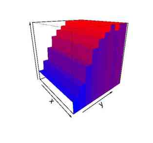
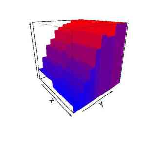
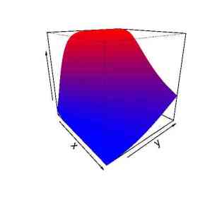
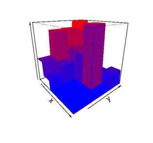
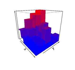
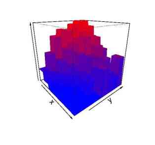
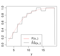
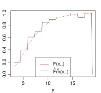
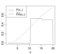
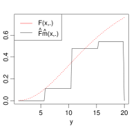
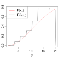
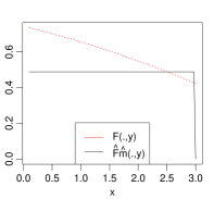
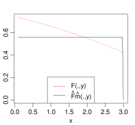
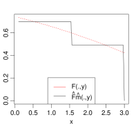
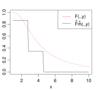
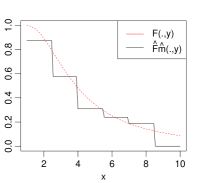
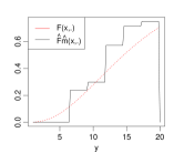
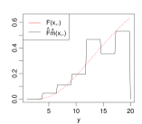
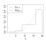
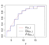
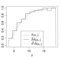
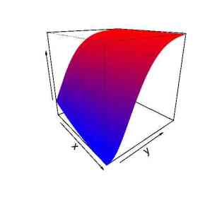
For models 1 and 2, samples (Xi,Yi,Ti)i=1,,nsubscriptsubscript𝑋𝑖subscript𝑌𝑖subscript𝑇𝑖𝑖1𝑛(X_{i},Y_{i},T_{i})_{i=1,\dots,n} of size n=(500,1000,5000)𝑛50010005000n=(500,1000,5000) are generated, and the model selection estimators F~m^subscript~𝐹^𝑚\tilde{F}_{\widehat{m}} is computed from the sample (Xi,Ti,δi=1I{YiTi})i=1,,nsubscriptsubscript𝑋𝑖subscript𝑇𝑖subscript𝛿𝑖1subscriptIsubscript𝑌𝑖subscript𝑇𝑖𝑖1𝑛(X_{i},T_{i},\delta_{i}=1\!\text{I}_{\{Y_{i}\leq T_{i}\}})_{i=1,\dots,n}. The results are displayed in Figure 1. Each row corresponds to a simulation model. The first column presents the target function F𝐹F and columns 2 to 4 present the estimators for sample size n=(500,1000,5000)𝑛50010005000n=(500,1000,5000). The same functions are plotted in Figures 2 and 3 for a fixed x𝑥x and y𝑦y respectively. As expected, the estimation gets better when the sample size increases, but we notice that a large sample size is required in order to get correct estimation. Indeed, on the one hand, the nature of the current status data provides less precise information about the variable of interest than uncensored of right-censored data, and on the other hand, the transition from uni- to bi-dimensional framework induces a loss in estimation quality for a given sample size.
Refer to caption Refer to caption Refer to caption Refer to caption
n=500𝑛500n=500 n=1000𝑛1000n=1000 n=5000𝑛5000n=5000
Figure 1: Conditional cumulative distribution function F𝐹F (first column) and model selection estimator F~m^subscript~𝐹^𝑚\tilde{F}_{\widehat{m}} for sample size n=(500,1000,5000)𝑛50010005000n=(500,1000,5000). First row: model 1; Second row: model 2.
Refer to caption Refer to caption Refer to caption
n=500𝑛500n=500 n=1000𝑛1000n=1000 n=5000𝑛5000n=5000
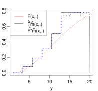
Figure 2: Model selection estimator F~m^subscript~𝐹^𝑚\tilde{F}_{\widehat{m}} (black solid line) and target function F𝐹F (red dotted line) for a fixed value of x𝑥x. First row: model 1, x=0.9𝑥0.9x=0.9; second row: model 2, x=5𝑥5x=5.
Refer to caption Refer to caption Refer to caption
n=500𝑛500n=500 n=1000𝑛1000n=1000 n=5000𝑛5000n=5000
Figure 3: Model selection estimator F~m^subscript~𝐹^𝑚\tilde{F}_{\widehat{m}}(black solid line) and target function F𝐹F (red dotted line) for a fixed value of y𝑦y. First row: model , y=7.5𝑦7.5y=7.5; Second row: model 2, y=10.5𝑦10.5y=10.5.

6.3 Impact of the distance between the densities of Y𝑌Y and T𝑇T

In a right-censoring framework, the rate of censoring, defined as the expected proportion of observations that are censored, is a well-known factor which impacts the quality of estimation: higher rate of censoring leads to poorer estimation. Indeed as the rate of censoring decreases, the proportion of survival times actually observed increases and the estimation of the survival time distribution gets better. In the current status data framework, the rate of censoring can not be defined since the survival time is never directly observed. In alternative, the distance between the densities of Y𝑌Y and T𝑇T appears as a relevant parameter that impacts the quality of estimation. Let us heuristically explain this idea.

First of all, the estimation of F𝐹F is more accurate if the observation times are concentrated in the areas where F𝐹F shows the highest variations. Besides, for a given value of the variable X𝑋X, the highest variations of the c.d.f. F𝐹F correspond to the largest values of the conditional density fY|Xsubscript𝑓conditional𝑌𝑋f_{Y|X}. Therefore, the estimation of F𝐹F improves as the densities of the observation time and survival time get closer, which may be quantified by the distance between the marginal densities fYsubscript𝑓𝑌f_{Y} and fTsubscript𝑓𝑇f_{T}. As a particular case, consider the situation when the supports of fYsubscript𝑓𝑌f_{Y} and fTsubscript𝑓𝑇f_{T} are disconnected: δisubscript𝛿𝑖\delta_{i} has the same value, either 0 or 1, for all i𝑖i; thus the observation set (Xi,Ti,δi)i=1,nsubscriptsubscript𝑋𝑖subscript𝑇𝑖subscript𝛿𝑖𝑖1𝑛(X_{i},T_{i},\delta_{i})_{i=1\dots,n} do not provide information about the distribution of Y𝑌Y. We enhance this heuristic on numerical examples.

Model 2b. We consider the same distribution as Model 2 except that an offset a𝑎a is added to Y𝑌Y:

(Mod 2b){XΓ(k=1.5,θ=2)Y=a+X×εwithεΓ(k=3,θ=1)T=X×εwithεΓ(k=3,θ=1)missing-subexpression(Mod 2b)casessimilar-to𝑋Γformulae-sequence𝑘1.5𝜃2formulae-sequence𝑌𝑎𝑋𝜀withsimilar-to𝜀Γformulae-sequence𝑘3𝜃1formulae-sequence𝑇𝑋superscript𝜀withsimilar-tosuperscript𝜀Γformulae-sequence𝑘3𝜃1\begin{array}[]{l}\\ \text{(Mod 2b)}\\ \\ \end{array}\left\{\begin{array}[]{l}X\sim\Gamma(k=1.5,\theta=2)\\ Y=a+X\times\varepsilon\quad\text{with}\quad\varepsilon\sim\Gamma(k=3,\theta=1)\\ T=X\times\varepsilon^{\prime}\quad\text{with}\quad\varepsilon^{\prime}\sim\Gamma(k=3,\theta=1)\\ \end{array}\right.

The conditional cumulative distribution function F(x,y)=ϕ(y/x,k=3,θ=1)F(x,y)=\phi(y/x,k=3,\theta=1) is estimated on the set A=[1,10]×[1,20]𝐴110120A=[1,10]\times[1,20]. The density f(X,T)subscript𝑓𝑋𝑇f_{(X,T)} is lower bounded by h0=107subscript0superscript107h_{0}=10^{-7} on A. We consider the L1𝐿1L1-distance between the densities of Y𝑌Y and T𝑇T:

dist(a)dist𝑎\displaystyle\text{dist}(a) =\displaystyle= fYfTL1=x=0+u=0+|fY|X(x,u)fT|X(x,u)|fX(x)𝑑x𝑑usubscriptnormsubscript𝑓𝑌subscript𝑓𝑇superscript𝐿1superscriptsubscript𝑥0superscriptsubscript𝑢0subscript𝑓conditional𝑌𝑋𝑥𝑢subscript𝑓conditional𝑇𝑋𝑥𝑢subscript𝑓𝑋𝑥differential-d𝑥differential-d𝑢\displaystyle\|f_{Y}-f_{T}\|_{L^{1}}=\int_{x=0}^{+\infty}\int_{u=0}^{+\infty}\left|f_{Y|X}(x,u)-f_{T|X}(x,u)\right|f_{X}(x)dxdu
=\displaystyle= x=0+u=a+|ϕ(uax,3,1)ϕ(ux,3,1)|ϕ(x,1.5,2)𝑑x𝑑usuperscriptsubscript𝑥0superscriptsubscript𝑢𝑎italic-ϕ𝑢𝑎𝑥31italic-ϕ𝑢𝑥31italic-ϕ𝑥1.52differential-d𝑥differential-d𝑢\displaystyle\int_{x=0}^{+\infty}\int_{u=a}^{+\infty}\left|\phi\left(\frac{u-a}{x},3,1\right)-\phi\left(\frac{u}{x},3,1\right)\right|\phi(x,1.5,2)dxdu

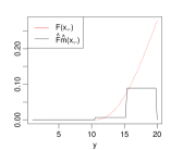
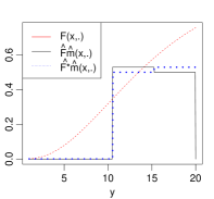
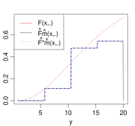
The values of dist(a)dist𝑎\text{dist}(a) for a=(0,2,5,10)𝑎02510a=(0,2,5,10) are displayed in Table 1. For each value of a𝑎a, a sample (Xi,Yi,Ti)i=1,,nsubscriptsubscript𝑋𝑖subscript𝑌𝑖subscript𝑇𝑖𝑖1𝑛(X_{i},Y_{i},T_{i})_{i=1,\dots,n} of size n=3000𝑛3000n=3000 is generated from Model 2b, and the model selection estimator is computed on the set A=[1,10]×[1,20]𝐴110120A=[1,10]\times[1,20]. The results are presented in Figure 4. A degradation in the estimation is observed as the distance between the densities of Y𝑌Y and T𝑇T increases. In particular, for a=10𝑎10a=10, dist(a𝑎a) gets close to 2, which indicates that the supports of the distribution of Y𝑌Y and T𝑇T hardly overlap, and the estimation is very poor despite a large sample size.

a𝑎a 0 2 5 10
dist(a𝑎a) 0 0.63 1.12 1.54
Table 1: L1superscript𝐿1L^{1}-distance between fYsubscript𝑓𝑌f_{Y} and fTsubscript𝑓𝑇f_{T} for an offset a𝑎a.
Refer to caption Refer to caption Refer to caption Refer to caption
a=0𝑎0a=0 a=2𝑎2a=2 a=5𝑎5a=5 a=10𝑎10a=10
Figure 4: Results on simulation from Model 2b with offset a=(0,2,5,10)𝑎02510a=(0,2,5,10); model selection estimator (black solid line) and target function F𝐹F (red dotted line) for a fixed value of x𝑥x, x=5.5𝑥5.5x=5.5. .

6.4 Increasing rearrangement

The results displayed on Figure 2 enhance that the estimate of F𝐹F is not necessarily increasing with respect to the second variable. Indeed the mean-square estimation does not account for the monotonicity of the c.d.f. The quality of estimation can be improved by monotonizing the model selection estimator F~m^subscript~𝐹^𝑚\tilde{F}_{\widehat{m}}. For an univariate function hh defined on [0,1]01[0,1], Chernozhukov et al. (2007) propose a rearrangement based on the following observation: if hh was non-decreasing, the quantile function of the random variable h(U)𝑈h(U) with U𝑈U uniformly distributed on [0,1]01[0,1] would be equal to hh. Therefore, the rearrangement hsuperscripth^{*} of hh is defined as the quantile function of h(U)𝑈h(U):

h(y)=inf{z,(011I{h(u)z}𝑑u)y}.superscript𝑦infimumformulae-sequence𝑧superscriptsubscript011subscriptI𝑢𝑧differential-d𝑢𝑦h^{*}(y)=\inf\left\{z\in\mathbb{R},\left(\int_{0}^{1}1\!\text{I}_{\{h(u)\leq z\}}du\right)\geq y\right\}.

For each xA1𝑥subscript𝐴1x\in A_{1}, we implement this procedure to the marginal function yF~m^(x,y)𝑦subscript~𝐹^𝑚𝑥𝑦y\rightarrow\tilde{F}_{\widehat{m}}(x,y) up to an affine substitution of variable which transform A2=[a,b]subscript𝐴2𝑎𝑏A_{2}=[a,b] into [0,1]01[0,1]. Namely,

F~m^(x,y)=inf{z,(ab1I{F~m^(x,u)z}𝑑u)ya},(x,y)A.formulae-sequencesuperscriptsubscript~𝐹^𝑚𝑥𝑦infimumformulae-sequence𝑧superscriptsubscript𝑎𝑏1subscriptIsubscript~𝐹^𝑚𝑥𝑢𝑧differential-d𝑢𝑦𝑎for-all𝑥𝑦𝐴\tilde{F}_{\widehat{m}}^{*}(x,y)=\inf\left\{z\in\mathbb{R},\left(\int_{a}^{b}1\!\text{I}_{\{\tilde{F}_{\widehat{m}}(x,u)\leq z\}}du\right)\geq y-a\right\},\quad\forall(x,y)\in A. (18)

In the numerical implementation, the infimum in (18) is taken over the range of values of F~m^(x,)subscript~𝐹^𝑚𝑥\tilde{F}_{\widehat{m}}(x,\cdot). Moreover, as F~m^subscript~𝐹^𝑚\tilde{F}_{\widehat{m}} is piecewise constant, the rearrangement is identical on each interval and only a finite number of rearrangement has to be computed. The results are presented on Figure 5.

By construction the function F~m^superscriptsubscript~𝐹^𝑚\tilde{F}_{\widehat{m}}^{*} is increasing with respect to the second variable. Moreover, according to Proposition 1 in Chernozhukov et al. (2007), the rearranged estimate presents a smaller L2superscript𝐿2L^{2}-error than the initial estimate: for every xA1𝑥subscript𝐴1x\in A_{1},

A2(F~m^(x,y)F(x,y))2𝑑yA2(F~m^(x,y)F(x,y))2𝑑ya.s.formulae-sequencesubscriptsubscript𝐴2superscriptsuperscriptsubscript~𝐹^𝑚𝑥𝑦𝐹𝑥𝑦2differential-d𝑦subscriptsubscript𝐴2superscriptsubscript~𝐹^𝑚𝑥𝑦𝐹𝑥𝑦2differential-d𝑦𝑎𝑠\int_{A_{2}}\left(\tilde{F}_{\widehat{m}}^{*}(x,y)-F(x,y)\right)^{2}dy\leq\int_{A_{2}}\left(\tilde{F}_{\widehat{m}}(x,y)-F(x,y)\right)^{2}dy\quad a.s. (19)

Thus the rearrangement brings an improvement in terms of L2superscript𝐿2L^{2}-risk.

Refer to caption Refer to caption Refer to caption
n=500𝑛500n=500 n=1000𝑛1000n=1000 n=5000𝑛5000n=5000
Figure 5: Model selection estimator F~m^subscript~𝐹^𝑚\tilde{F}_{\widehat{m}} (black solid line), rearranged estimator F~m^superscriptsubscript~𝐹^𝑚\tilde{F}_{\widehat{m}}^{*} (blue dotted line) and target function F𝐹F (red dashed line) for a fixed value of x𝑥x. First row: model 1, x=0.9𝑥0.9x=0.9; second row: model 2, x=5𝑥5x=5.

7 Discussion

7.1 Summary of the results

In the interval censoring framework, case 1, Brunel and Comte (2009) observe that the c.d.f. is equal to the regression function of the observation times over the indicators and propose an estimator of the c.d.f. computed by minimization of a least-square contrast on a collection of linear models followed by a model selection procedure. In this paper, we extend this approach to conditional c.d.f. via a collection of two-dimensional linear models built as tensor products of uni-dimensional ones. The inclusion of a covariate does not give rise to specific technical difficulties, but in order to emphasize the role played by each hypothesis, we adopt a different presentation of the results which leads to changes in the proofs.

First of all, an oracle inequality for the empirical risk conditional to the observations (𝐗,𝐓)𝐗𝐓({\bf X,T}) is stated. This result only requires a limitation of the number of models in the collection with a given dimension and is valid regardless of the regularity of the variables. Besides, it directly handles the fix-designed context with non-random observation times and covariates. The main difference in the proof is the use of a concentration inequality for empirical process with independent but non identically distributed variables. An oracle inequality for the L2superscript𝐿2L^{2}-risk on a restricted set A×+𝐴superscriptA\in\mathbb{R}\times\mathbb{R}^{+} is then derived under additional assumptions. First of all, the density f(X,T)subscript𝑓𝑋𝑇f_{(X,T)} is assumed to be bounded on A𝐴A in order to guarantee the equivalence between the empirical and L2superscript𝐿2L^{2}-norms; this condition is inherent to the design since the c.d.f can only be estimated on a set with sufficiently concentrated observations. Moreover, the construction of our collection of models by tensor product requires the set A𝐴A to be a product of intervals.

The oracle inequalities state the adaptivity of the model selection estimator over the collection of models. In order to demonstrate the optimality in a more general sense, a minimax study is conducted over anisotropic Besov balls. The rate is characteristic of regression estimation but differs from the rate obtained on right-censored data.

A numerical study on simulated data with additive and multiplicative effects of the covariate is presented. We observe that a large sample size is necessary in order to get acceptable quality of estimation, due on the one hand to the multi-dimensional context, and on the other hand to the current status data framework in which poor information is brought by the censoring indicator. Besides, in alternative to the censoring rate usually considered in right-censoring, we emphasize the impact of the distance between the densities of the survival and observation times on the quality of estimation: closer densities lead to a better estimation.

7.2 Extension to multi-dimensional covariates

From a theoretical point of view, the procedure presented in this paper could be extended to covariates Xk𝑋superscript𝑘X\in\mathbb{R}^{k} with k2𝑘2k\geq 2 by building a collection of models from multiple tensor products. For an index m=(m1,,mk+1)𝑚subscript𝑚1subscript𝑚𝑘1m=(m_{1},\dots,m_{k+1}), the following model would be considered:

Sm=Sm1(1)Smk+1(k+1)subscript𝑆𝑚tensor-productsuperscriptsubscript𝑆subscript𝑚11subscriptsuperscript𝑆𝑘1subscript𝑚𝑘1S_{m}=S_{m_{1}}^{(1)}\otimes\dots\otimes S^{(k+1)}_{m_{k+1}}

with Sm1(1),,Smk(k)superscriptsubscript𝑆subscript𝑚11subscriptsuperscript𝑆𝑘subscript𝑚𝑘S_{m_{1}}^{(1)},\dots,S^{(k)}_{m_{k}} linear subspaces of L2()superscript𝐿2L^{2}(\mathbb{R}) and Smk+1(k+1)subscriptsuperscript𝑆𝑘1subscript𝑚𝑘1S^{(k+1)}_{m_{k+1}} linear subspace of L2(+)superscript𝐿2superscriptL^{2}(\mathbb{R}^{+}).

Nevertheless the simulation study with a uni-dimensional covariate emphasizes the necessity of a large sample, and additional covariates could only be considered in situations with a large sample available. Besides the control of the integrated risk requires restrictions on the maximum dimension of the models. Let Nn()superscriptsubscript𝑁𝑛N_{n}^{(\ell)} be the maximum dimension of Sm()subscriptsuperscript𝑆subscript𝑚S^{(\ell)}_{m_{\ell}} for =1,,k+11𝑘1\ell=1,\dots,k+1, assumption (A2)subscriptA2(\textbf{A}_{2}) turns into:

Nn(1)××Nn(k+1)nlogn.superscriptsubscript𝑁𝑛1superscriptsubscript𝑁𝑛𝑘1𝑛𝑛N_{n}^{(1)}\times\dots\times N_{n}^{(k+1)}\leq\sqrt{\frac{n}{\log n}}. (20)

which is satisfied as soon as:

Nn()(nlogn)1/2(k+1),=1,,k+1.formulae-sequencesuperscriptsubscript𝑁𝑛superscript𝑛𝑛12𝑘1for-all1𝑘1N_{n}^{(\ell)}\leq\left(\frac{n}{\log n}\right)^{1/2(k+1)},\quad\forall\ell=1,\dots,k+1.

Assume that F𝐹F is in 2,β(A,L)superscriptsubscript2𝛽𝐴𝐿\mathcal{B}_{2,\infty}^{\beta}(A,L) the anisotropic Besov ball of regularity β=(β1,,βk+1)𝛽subscript𝛽1subscript𝛽𝑘1\beta=(\beta_{1},\dots,\beta_{k+1}) on L2(k×+)superscript𝐿2superscript𝑘superscriptL^{2}(\mathbb{R}^{k}\times\mathbb{R}^{+}). Under condition (20), similarly to (17), the model selection estimator satisfies the following inequality.

𝔼[F~m^F2]𝔼delimited-[]superscriptnormsubscript~𝐹^𝑚𝐹2\displaystyle\mathbb{E}\left[\|\tilde{F}_{\widehat{m}}-F\|^{2}\right]
C{(Dm1(1))2β1++(Dmk+1(k+1))2βk+1+Dm1(1)Dmk+1(k+1)n}+Cnabsent𝐶superscriptsuperscriptsubscript𝐷subscript𝑚112subscript𝛽1superscriptsuperscriptsubscript𝐷subscript𝑚𝑘1𝑘12subscript𝛽𝑘1superscriptsubscript𝐷subscript𝑚11superscriptsubscript𝐷subscript𝑚𝑘1𝑘1𝑛superscript𝐶𝑛\displaystyle\leq C\left\{\left(D_{m_{1}}^{(1)}\right)^{-2\beta_{1}}+\dots+\left(D_{m_{k+1}}^{(k+1)}\right)^{-2\beta_{k+1}}+\frac{D_{m_{1}}^{(1)}\dots D_{m_{k+1}}^{(k+1)}}{n}\right\}+\frac{C^{\prime}}{n} (21)

with Dm()superscriptsubscript𝐷subscript𝑚D_{m_{\ell}}^{(\ell)} the dimension of Sm()subscriptsuperscript𝑆subscript𝑚S^{(\ell)}_{m_{\ell}}. Thus, the model m¯=(m¯1,,m¯k+1)¯𝑚subscript¯𝑚1subscript¯𝑚𝑘1\overline{m}=(\overline{m}_{1},\dots,\overline{m}_{k+1}) which realizes the trade-off in (7.2) satisfies:

Dm¯()n1/(2β(1+j=1k+1(2βj)1).D_{\overline{m}_{\ell}}^{(\ell)}\propto n^{1/(2\beta_{\ell}(1+\sum_{j=1}^{k+1}(2\beta_{j})^{-1})}. (22)

Conditions (20) and (22) are satisfied as soon as β>(k+1)/2subscript𝛽𝑘12\beta_{\ell}>(k+1)/2 for every =1,,k+11𝑘1\ell=1,\dots,k+1, and the rate of convergence is n2β¯/(2β¯+(k+1))superscript𝑛2¯𝛽2¯𝛽𝑘1n^{-2\overline{\beta}/(2\overline{\beta}+(k+1))} with β¯¯𝛽\overline{\beta} the harmonic mean. Therefore, the regularity conditions which guarantee the minimax adaptivity get stronger and the rate of convergence decreases as the dimension of the covariate increases.

7.3 Contribution with respect to extant literature

Most estimation procedures developed for current status data are based on the NPMLE originally proposed by Groeneboom and Wellner (1992) and the covariates are usually handled through semi-parametric models (e.g. Cheng and Wang (2011)). Minimax results are assessed under the assumption of a continuous density for the survival and observation times (van de Geer (1993)). Nevertheless, very few adaptive procedures are proposed and they do not include covariates. In alternative to the NPMLE, Ma and Kosorok (2006) and Brunel and Comte (2009) enlighten the parallel between regression and current status data frameworks and propose several adaptive estimation procedures adapted from regression analysis, which exhibit rates of convergence typical of a regression context.

In this paper, we develop the mean-square procedure from Brunel and Comte (2009). Our first contribution is the inclusion of a covariate in a nonparametric adaptive estimation procedure. The second improvement is the computation of the minimax rate over anisotropic Besov balls which assesses the optimality of the regression-type approach in the current status setting; the minimax rate for independent survival and observation times can be derived as a particular case, proving the minimaxicity of the mean-square estimator from Brunel and Comte (2009).

7.4 Perspectives

The parallel between current status and regression frameworks would allow the implementation of other adaptive methods. We briefly present some advantages and drawbacks of alternative approaches that may be considered.

Lepski’s method provides locally minimax results up to a logarithm loss unavoidable in pointwise adaptive procedures, and more recent developments display oracle inequalities. Adaptation over classes of regularity is achieved through a bias-variance compromise from kernel estimators (Lepski (1991)). Goldenshluger and Lepski (2008) propose a modification of the original method based on the ordering of the classes of regularity in order to estimate multi-dimensional function in a gaussian regression framework. Adaptation of this procedure for current status data framework is conceivable, but as for model selection, a specific study of the upper-bound would be necessary. Besides, the implementation of Lepski’s procedure presents a high computational complexity, especially in mullti-dimensional context. Since the estimation of the conditional c.d.f. from current status data requires large sample size, more easily computable methods may be preferred. However, Lepski’s method allows local adaptivity which may be favoured when the target function present irregular smoothness.

Wavelet thresholding methods are widely used in practical situations, in particular in signal processing. The procedure consists in a decomposition in a multi-scale wavelet basis followed by a thresholding of the smallest coefficients. The estimators reach the minimax rate of convergence over various classes of regularity, usually up to a logarithm loss (e.g. Kerkyacharian and Picard (2004)). Massart (2007) demonstrates the equivalence between wavelet thresholding and the complete variable selection procedure which falls into the model selection framework with a collection including a large number of models with the same dimension. Therefore, following the adaptation of tools developed for regression estimation by model selection to the current status framework, wavelet thresholding could be developed in future research.

The mean-square contrast is naturally adapted to the empirical norm and additional assumptions are required for the control of the L2superscript𝐿2L^{2}-risk. Conversely, quotient regression estimators presented e.g. in Tsybakov (2004) are directly adapted to the L2superscript𝐿2L^{2} norm. Brunel and Comte (2009) show that the rate of convergence of the model selection quotient estimator from current status data depends on the minimum regularity of the c.d.f. and the observation time density. Therefore, this procedure does not reach the minimax rate if the c.d.f. is smoother than the observation time.

As the conditional c.d.f. lies into [0,1]01[0,1], procedures for bounded regression may be considered. In particular, we present a comparison of our method with the model selection framework for bounded regression proposed by Massart (2007). The general assumptions are less restrictive than in the classical regression framework since the errors are not supposed to be independent from the design, but the procedure requires models which consist of bounded functions. Two types of bounded models could be directly derived from the linear models {Sm,mIn}subscript𝑆𝑚𝑚subscript𝐼𝑛\{S_{m},m\in I_{n}\}:

  • 1.

    Thresholded linear models: S~m(1)={t~=max(min(t,1),0),tSm}superscriptsubscript~𝑆𝑚1formulae-sequence~𝑡𝑡10𝑡subscript𝑆𝑚\tilde{S}_{m}^{(1)}=\{\tilde{t}=\max(\min(t,1),0),t\in S_{m}\}

  • 2.

    Restricted linear models: S~m(2)={tSm,t(x)[0,1],x}superscriptsubscript~𝑆𝑚2formulae-sequence𝑡subscript𝑆𝑚𝑡𝑥01for-all𝑥\tilde{S}_{m}^{(2)}=\{t\in S_{m},t(x)\in[0,1],\forall x\}.

We present a brief overview of the advantages and difficulties encountered in the implementation of these models on the interval censoring design. According to Theorem 8.5 in Massart (2007), for each model m𝑚m, two quantities have to be controlled in order to obtain minimax results: 1/ the stochastic modulus of uniform continuity ϕmsubscriptitalic-ϕ𝑚\phi_{m} of the centered empirical process, 2/ the bias term via results of approximation on regularity spaces. On the one hand, the bias term for S~m(1)superscriptsubscript~𝑆𝑚1\tilde{S}_{m}^{(1)} is directly controlled by results on linear models, but since the unit ball of S~m(1)superscriptsubscript~𝑆𝑚1\tilde{S}_{m}^{(1)} is larger than the one of Smsubscript𝑆𝑚S_{m}, the computation of the function ϕmsubscriptitalic-ϕ𝑚\phi_{m} requires a specific study. On the other hand, as S~m(2)superscriptsubscript~𝑆𝑚2\tilde{S}_{m}^{(2)} is included in Smsubscript𝑆𝑚S_{m}, ϕmsubscriptitalic-ϕ𝑚\phi_{m} can directly be deduced from results on linear models, but the bias term which involved the L2superscript𝐿2L^{2}-projection of F𝐹F on Lsuperscript𝐿L^{\infty}-balls does not falls into classical approximation setting.

Besides, an alternative procedure based on finite models, originally developed by Massart (2007) in a Gaussian framework (Chapter 4), could be considered in order to include bounded models. For every α>0𝛼0\alpha>0, a net of radius α𝛼\alpha is extracted from a set of function 𝒮𝒮\mathcal{S} including the target function. An appropriate choice of radii {αm,mIn}subscript𝛼𝑚𝑚subscript𝐼𝑛\{\alpha_{m},m\in I_{n}\} based on wavelet or polynomial characterization of Besov classes provides minimax estimation.

Thus, our model selection procedure takes advantage of classical tools for the control of the deviation of empirical process on linear models as well as extant results of approximation on Besov spaces, but does not directly fit into the bounded regression framework. Alternative approaches using bounded models could be considered for future research, but give rise to other technical difficulties than the one encountered with linear models.

7.5 Conclusion

The model selection mean-square estimator of the conditional c.d.f. satisfies non-asymptotic adaptivity on a collection of models, as well as minimaxity. The control of the upper-bound takes advantages of the tools used in classical regression. Furthermore, our results underline the optimality of the regression-type approach, which establishes a connection between the interval censoring framework and the widely developed field of regression estimation and makes the way for the adaptation of regression methods to current status design.

8 Proofs

8.1 Talagrand Inequality

The risk of the model selection estimator is controlled with the following concentration inequality based on results from Talagrand (1996).

Theorem 8.1.

Let (V1,,Vn)subscript𝑉1subscript𝑉𝑛(V_{1},\dots,V_{n}) be independent random variables, and \mathcal{F} be a countable set of applications from \mathbb{R} to nsuperscript𝑛\mathbb{R}^{n} such that for every f𝑓f\in\mathcal{F}, the function f𝑓-f defined as (f)(x)=(f(x))𝑓𝑥𝑓𝑥(-f)(x)=-(f(x)) for every x𝑥x is in \mathcal{F} as well. Let

Z=supf|1ni=1n(f(i)(Vi)𝔼[f(i)(Vi)])|𝑍subscriptsupremum𝑓1𝑛superscriptsubscript𝑖1𝑛superscript𝑓𝑖subscript𝑉𝑖𝔼delimited-[]superscript𝑓𝑖subscript𝑉𝑖Z=\sup_{f\in\mathcal{F}}\left|\frac{1}{n}\sum_{i=1}^{n}(f^{(i)}(V_{i})-\mathbb{E}[f^{(i)}(V_{i})])\right|

and b𝑏b, v𝑣v and \mathbb{H} be such that

supf(supi=1,,nf(i))b,supf1ni=1nVar(f(i)(Vi))vand𝔼Z.formulae-sequencesubscriptsupremum𝑓subscriptsupremum𝑖1𝑛subscriptnormsuperscript𝑓𝑖𝑏formulae-sequencesubscriptsupremum𝑓1𝑛superscriptsubscript𝑖1𝑛𝑉𝑎𝑟superscript𝑓𝑖subscript𝑉𝑖𝑣and𝔼𝑍\sup_{f\in\mathcal{F}}\left(\sup_{i=1,\dots,n}\|f^{(i)}\|_{\infty}\right)\leq b,\quad\sup_{f\in\mathcal{F}}\frac{1}{n}\sum_{i=1}^{n}Var(f^{(i)}(V_{i}))\leq v\quad\text{and}\quad\mathbb{E}Z\leq\mathbb{H}.

Then, for every θ>1𝜃1\theta>1, there exists C¯¯𝐶\overline{C}, C¯superscript¯𝐶\overline{C}^{\prime}, K¯¯𝐾\overline{K}, K¯superscript¯𝐾\overline{K}^{\prime} such that for every n𝑛n,

𝔼[(Z2θ2)+]C¯vnexp(κ¯n2v)+C¯b2n2exp(κ¯nb)𝔼delimited-[]subscriptsuperscript𝑍2𝜃superscript2¯𝐶𝑣𝑛¯𝜅𝑛superscript2𝑣superscript¯𝐶superscript𝑏2superscript𝑛2superscript¯𝜅𝑛𝑏\mathbb{E}\left[(Z^{2}-\theta\mathbb{H}^{2})_{+}\right]\leq\overline{C}\frac{v}{n}\exp\left(-\overline{\kappa}\frac{n\mathbb{H}^{2}}{v}\right)+\overline{C}^{\prime}\frac{b^{2}}{n^{2}}\exp\left(-\overline{\kappa}^{\prime}\frac{n\mathbb{H}}{b}\right)

Theorem 8.1 is derived from Theorem 1.1 in Klein and Rio (2005) by setting s(i)(t)=1b(f(i)(t)𝔼[f(i)(Vi)])superscript𝑠𝑖𝑡1𝑏superscript𝑓𝑖𝑡𝔼delimited-[]superscript𝑓𝑖subscript𝑉𝑖s^{(i)}(t)=\frac{1}{b}(f^{(i)}(t)-\mathbb{E}[f^{(i)}(V_{i})]). Similarly to Birgé and Massart (1998), Corollary 2, we get

P[Z(1+ν)+x]exp(n3min(y22v,2min(1,ν)y7b)).𝑃delimited-[]𝑍1𝜈𝑥𝑛3superscript𝑦22𝑣21𝜈𝑦7𝑏P[Z\geq(1+\nu)\mathbb{H}+x]\leq\exp\left(-\frac{n}{3}\min\left(\frac{y^{2}}{2v},\frac{2\min(1,\nu)y}{7b}\right)\right).

Then we use the formula 𝔼[X+]0+P[Xs]𝑑s𝔼delimited-[]subscript𝑋superscriptsubscript0𝑃delimited-[]𝑋𝑠differential-d𝑠\mathbb{E}[X_{+}]\leq\int_{0}^{+\infty}P[X\geq s]ds to get

𝔼[(Z2θ2)+]0+P[Zθ2+s]𝑑s0+P[Zα1+α2+α3s]𝑑s𝔼delimited-[]subscriptsuperscript𝑍2𝜃superscript2superscriptsubscript0𝑃delimited-[]𝑍𝜃superscript2𝑠differential-d𝑠superscriptsubscript0𝑃delimited-[]𝑍subscript𝛼1subscript𝛼2subscript𝛼3𝑠differential-d𝑠\mathbb{E}\left[(Z^{2}-\theta\mathbb{H}^{2})_{+}\right]\leq\int_{0}^{+\infty}\!\!\!P[Z\geq\sqrt{\theta\mathbb{H}^{2}+s}]ds\leq\int_{0}^{+\infty}\!\!\!P[Z\geq\alpha_{1}\mathbb{H}+\sqrt{\alpha_{2}\mathbb{H}+\alpha_{3}s}]ds

for some positive (α1,α2,α3)subscript𝛼1subscript𝛼2subscript𝛼3(\alpha_{1},\alpha_{2},\alpha_{3}), and a simple integration provides the result of Theorem 8.1.

8.2 Proof of Theorem 4.1.

The proof is similar to Brunel and Comte (2009), Section 6.4, but the conditional empirical norm is considered instead of the L2superscript𝐿2L^{2} one. This modification entails changes in the proofs that are displayed in this section. The vectors 𝐗𝐗{\bf X} and 𝐓𝐓{\bf T} are assumed to be fixed along this section. Let mIn𝑚subscript𝐼𝑛m\in I_{n} and FmSmsubscript𝐹𝑚subscript𝑆𝑚F_{m}\in S_{m}, by definition of F^msubscript^𝐹𝑚\widehat{F}_{m} and m^^𝑚\widehat{m},

F^mFn2superscriptsubscriptnormsubscript^𝐹𝑚𝐹𝑛2\displaystyle\|\widehat{F}_{m}-F\|_{n}^{2} \displaystyle\leq FmFn2+pen(m)pen(m^)+2νn(F^m^Fm)superscriptsubscriptnormsubscript𝐹𝑚𝐹𝑛2𝑝𝑒𝑛𝑚𝑝𝑒𝑛^𝑚2subscript𝜈𝑛subscript^𝐹^𝑚subscript𝐹𝑚\displaystyle\|F_{m}-F\|_{n}^{2}+pen(m)-pen(\widehat{m})+2\nu_{n}(\widehat{F}_{\widehat{m}}-F_{m})
\displaystyle\leq FmFn2+pen(m)pen(m^)+F^mFmnsuptSm+Sm^,tn1|νn(t)|superscriptsubscriptnormsubscript𝐹𝑚𝐹𝑛2𝑝𝑒𝑛𝑚𝑝𝑒𝑛^𝑚subscriptnormsubscript^𝐹𝑚subscript𝐹𝑚𝑛subscriptsupremumformulae-sequence𝑡subscript𝑆𝑚subscript𝑆^𝑚subscriptnorm𝑡𝑛1subscript𝜈𝑛𝑡\displaystyle\|F_{m}-F\|_{n}^{2}+pen(m)-pen(\widehat{m})+\|\widehat{F}_{m}-F_{m}\|_{n}\sup_{t\in S_{m}+S_{\widehat{m}},\|t\|_{n}\leq 1}\!\!\!|\nu_{n}(t)|

with νnsubscript𝜈𝑛\nu_{n} defined in (9). Let θ=θ1/3>1superscript𝜃superscript𝜃131\theta^{\prime}=\theta^{1/3}>1, and p(m,m)=θ(Dm+Dm)/(4n)𝑝𝑚superscript𝑚superscript𝜃subscript𝐷𝑚subscript𝐷superscript𝑚4𝑛p(m,m^{\prime})=\theta^{\prime}(D_{m}+D_{m^{\prime}})/(4n). We recall that for every (x,y)2𝑥𝑦superscript2(x,y)\in\mathbb{R}^{2}, 2xyx2/θ2+θ2y22𝑥𝑦superscript𝑥2superscript𝜃2superscript𝜃2superscript𝑦22xy\leq x^{2}/\theta^{\prime 2}+\theta^{\prime 2}y^{2} and (x+y)2θx2+(1+1/(θ1))y2superscript𝑥𝑦2superscript𝜃superscript𝑥211superscript𝜃1superscript𝑦2(x+y)^{2}\leq\theta^{\prime}x^{2}+(1+1/(\theta^{\prime}-1))y^{2}. Therefore,

F^mFn2superscriptsubscriptnormsubscript^𝐹𝑚𝐹𝑛2\displaystyle\|\widehat{F}_{m}-F\|_{n}^{2} \displaystyle\leq FmFn2+pen(m)pen(m^)+θ2p(m,m^)+1θ2F^mFmn2superscriptsubscriptnormsubscript𝐹𝑚𝐹𝑛2𝑝𝑒𝑛𝑚𝑝𝑒𝑛^𝑚superscript𝜃2𝑝𝑚^𝑚1superscript𝜃2superscriptsubscriptnormsubscript^𝐹𝑚subscript𝐹𝑚𝑛2\displaystyle\|F_{m}-F\|_{n}^{2}+pen(m)-pen(\widehat{m})+\theta^{\prime 2}p(m,\widehat{m})+\frac{1}{\theta^{\prime 2}}\|\widehat{F}_{m}-F_{m}\|_{n}^{2}
+θ2suptSm+Sm^,tn1((νn(t))2p(m,m^))superscript𝜃2subscriptsupremumformulae-sequence𝑡subscript𝑆𝑚subscript𝑆^𝑚subscriptnorm𝑡𝑛1superscriptsubscript𝜈𝑛𝑡2𝑝𝑚^𝑚\displaystyle+\theta^{\prime 2}\sup_{t\in S_{m}+S_{\widehat{m}},\|t\|_{n}\leq 1}\left((\nu_{n}(t))^{2}-p(m,\widehat{m})\right)
\displaystyle\leq FmFn2+2pen(m)superscriptsubscriptnormsubscript𝐹𝑚𝐹𝑛22𝑝𝑒𝑛𝑚\displaystyle\|F_{m}-F\|_{n}^{2}+2pen(m)
+1θ2(F^mFn2+θ(1+1θ1)FmFn2)1superscript𝜃2superscriptsubscriptnormsubscript^𝐹𝑚𝐹𝑛2superscript𝜃11superscript𝜃1superscriptsubscriptnormsubscript𝐹𝑚𝐹𝑛2\displaystyle+\frac{1}{\theta^{\prime 2}}\left(\|\widehat{F}_{m}-F\|_{n}^{2}+\theta^{\prime}\left(1+\frac{1}{\theta^{\prime}-1}\right)\|F_{m}-F\|_{n}^{2}\right)
+θ2mInsuptSm+Sm,tn1((νn(t))2p(m,m))superscript𝜃2subscriptsuperscript𝑚subscript𝐼𝑛subscriptsupremumformulae-sequence𝑡subscript𝑆𝑚subscript𝑆superscript𝑚subscriptnorm𝑡𝑛1superscriptsubscript𝜈𝑛𝑡2𝑝𝑚superscript𝑚\displaystyle+\theta^{\prime 2}\sum_{m^{\prime}\in I_{n}}\sup_{t\in S_{m}+S_{m^{\prime}},\|t\|_{n}\leq 1}\left((\nu_{n}(t))^{2}-p(m,m^{\prime})\right)

The end of the proof is provided by Theorem 8.1. According to the comment in Section 3.2, the supremum of νnsubscript𝜈𝑛\nu_{n} over the .n\|.\|_{n}-unit ball of Sm+Smsubscript𝑆𝑚subscript𝑆superscript𝑚S_{m}+S_{m^{\prime}} is equal to the supremum over the unit ball m+msuperscriptsubscript𝑚superscript𝑚\mathcal{B}_{m+m^{\prime}}^{*} of (Sm+Sm)superscriptsubscript𝑆𝑚subscript𝑆superscript𝑚(S_{m}+S_{m^{\prime}})^{*}. Let {φλ,λJm+m}subscript𝜑𝜆𝜆superscriptsubscript𝐽𝑚superscript𝑚\{\varphi_{\lambda},\lambda\in J_{m+m^{\prime}}^{*}\} be a .n\|.\|_{n}-orthogonal basis of (Sm+Sm)superscriptsubscript𝑆𝑚subscript𝑆superscript𝑚(S_{m}+S_{m^{\prime}})^{*}, by Cauchy-Schwartz Inequality and equation (10),

𝔼[suptm+m(νn(t))2|(𝐗,𝐓)]𝔼[supλJm+m(νn(φλ))2|(𝐗,𝐓)]Dm+Dm4n=2.𝔼delimited-[]conditionalsubscriptsupremum𝑡superscriptsubscript𝑚superscript𝑚superscriptsubscript𝜈𝑛𝑡2𝐗𝐓𝔼delimited-[]conditionalsubscriptsupremum𝜆superscriptsubscript𝐽𝑚superscript𝑚superscriptsubscript𝜈𝑛subscript𝜑𝜆2𝐗𝐓subscript𝐷𝑚subscript𝐷superscript𝑚4𝑛superscript2\mathbb{E}\left[\sup_{t\in\mathcal{B}_{m+m^{\prime}}^{*}}(\nu_{n}(t))^{2}|({\bf X,T})\right]\leq\mathbb{E}\left[\sup_{\lambda\in J_{m+m^{\prime}}^{*}}(\nu_{n}(\varphi_{\lambda}))^{2}|({\bf X,T})\right]\leq\frac{D_{m}+D_{m^{\prime}}}{4n}=\mathbb{H}^{2}. (23)

Moreover, for every tm+m𝑡superscriptsubscript𝑚superscript𝑚t\in\mathcal{B}_{m+m^{\prime}}^{*} and i{1,,n}𝑖1𝑛i\in\{1,\dots,n\},

|δit(Xi,Ti)||t(Xi,Ti)|ntnn=b.subscript𝛿𝑖𝑡subscript𝑋𝑖subscript𝑇𝑖𝑡subscript𝑋𝑖subscript𝑇𝑖𝑛subscriptnorm𝑡𝑛𝑛𝑏|\delta_{i}t(X_{i},T_{i})|\leq|t(X_{i},T_{i})|\leq\sqrt{n}\|t\|_{n}\leq\sqrt{n}=b. (24)

Finally, with a similar computation as (10), the supremum of the variance process is upper bounded by v=1/4𝑣14v=1/4. Therefore, Theorem 8.1 with the values of \mathbb{H}, b𝑏b and v𝑣v computed above concludes the proof of Theorem 4.1. \Box

8.3 Proof of Theorem 4.2

The proof is based on results presented by Baraud (2002) in a uni-dimensional context, but the demonstrations are identical for two-dimensional functions. Let ρ0>h01subscript𝜌0superscriptsubscript01\rho_{0}>h_{0}^{-1} and

Ωn={tn2t2ρ0,tSn}.subscriptΩ𝑛formulae-sequencesuperscriptsubscriptnorm𝑡𝑛2superscriptnorm𝑡2subscript𝜌0for-all𝑡subscript𝑆𝑛\Omega_{n}=\left\{\frac{\|t\|_{n}^{2}}{\|t\|^{2}}\leq\rho_{0},\ \forall t\in S_{n}\right\}.

On the one hand, according to Lemma 5.1 in Baraud (2002),

𝔼[F~m^F1IΩn]CinftSnFt2+𝔼[F~m^Fn2]𝔼delimited-[]normsubscript~𝐹^𝑚𝐹1subscriptIsubscriptΩ𝑛𝐶subscriptinfimum𝑡subscript𝑆𝑛superscriptnorm𝐹𝑡2𝔼delimited-[]superscriptsubscriptnormsubscript~𝐹^𝑚𝐹𝑛2\mathbb{E}\left[\|\tilde{F}_{\widehat{m}}-F\|1\!\text{I}_{\Omega_{n}}\right]\leq C\inf_{t\in S_{n}}\|F-t\|^{2}+\mathbb{E}\left[\|\tilde{F}_{\widehat{m}}-F\|_{n}^{2}\right] (25)

for some constant C𝐶C. Moreoever, by integrating (12) in Theorem 4.1, we obtain:

𝔼[F~m^Fn2]C1infmIn{inftSmh1Ft2+pen(m)}+C2n.𝔼delimited-[]superscriptsubscriptnormsubscript~𝐹^𝑚𝐹𝑛2subscript𝐶1subscriptinfimum𝑚subscript𝐼𝑛subscriptinfimum𝑡subscript𝑆𝑚subscript1superscriptnorm𝐹𝑡2𝑝𝑒𝑛𝑚subscript𝐶2𝑛\mathbb{E}\left[\|\tilde{F}_{\widehat{m}}-F\|_{n}^{2}\right]\leq C_{1}\inf_{m\in I_{n}}\left\{\inf_{t\in S_{m}}h_{1}\|F-t\|^{2}+pen(m)\right\}+\frac{C_{2}}{n}. (26)

Thus, as inftSnFt2inftSmFt2subscriptinfimum𝑡subscript𝑆𝑛superscriptnorm𝐹𝑡2subscriptinfimum𝑡subscript𝑆𝑚superscriptnorm𝐹𝑡2\inf_{t\in S_{n}}\|F-t\|^{2}\leq\inf_{t\in S_{m}}\|F-t\|^{2} for all mIn𝑚subscript𝐼𝑛m\in I_{n}, inequalities (25) and (26) entail:

𝔼[F~m^F1IΩn]CinfmIn{inftSmFt2+pen(m)}+C2n.𝔼delimited-[]normsubscript~𝐹^𝑚𝐹1subscriptIsubscriptΩ𝑛superscript𝐶subscriptinfimum𝑚subscript𝐼𝑛subscriptinfimum𝑡subscript𝑆𝑚superscriptnorm𝐹𝑡2𝑝𝑒𝑛𝑚subscript𝐶2𝑛\mathbb{E}\left[\|\tilde{F}_{\widehat{m}}-F\|1\!\text{I}_{\Omega_{n}}\right]\leq C^{\prime}\inf_{m\in I_{n}}\left\{\inf_{t\in S_{m}}\|F-t\|^{2}+pen(m)\right\}+\frac{C_{2}}{n}. (27)

On the other hand, according to Proposition 4.2 in Baraud (2002),

[Ωnc]C′′n.delimited-[]superscriptsubscriptΩ𝑛𝑐superscript𝐶′′𝑛\mathbb{P}\left[\Omega_{n}^{c}\right]\leq\frac{C^{\prime\prime}}{n}. (28)

Moreover, F~m^subscript~𝐹^𝑚\tilde{F}_{\widehat{m}} and F𝐹F lie into [0,1]01[0,1], therefore

F~m^Fh01F~m^FfX,Th01a.s.formulae-sequencenormsubscript~𝐹^𝑚𝐹superscriptsubscript01subscriptnormsubscript~𝐹^𝑚𝐹subscript𝑓𝑋𝑇superscriptsubscript01𝑎𝑠\|\tilde{F}_{\widehat{m}}-F\|\leq h_{0}^{-1}\|\tilde{F}_{\widehat{m}}-F\|_{f_{X,T}}\leq h_{0}^{-1}\quad a.s. (29)

Equations (27), (28) and (29) conclude the proof of Theorem 4.2. \Box

8.4 Proof of Theorem 5.1

The proof is based on the following theorem and lemma presented in Tsybakov (2004) (Theorem 2.5 and Lemma 2.7 in Chapter 2). Let =2,β(A,L)subscriptsuperscript𝛽2𝐴𝐿\mathcal{B}=\mathcal{B}^{\beta}_{2,\infty}(A,L). Denote by K(P,Q)𝐾𝑃𝑄K(P,Q) the Kullback distance between the distributions P𝑃P and Q𝑄Q:

K(P,Q)={log(dP/dQ)𝑑PifP<<Q+otherwise𝐾𝑃𝑄casesmuch-less-than𝑑𝑃𝑑𝑄differential-d𝑃if𝑃𝑄otherwiseK(P,Q)=\left\{\begin{array}[]{l}\int\log(dP/dQ)dP\quad\text{if}\quad P<<Q\\ +\infty\quad\text{otherwise}\end{array}\right.
Theorem 8.2.

Assume that there exist M2𝑀2M\geq 2 and F0,,FMsubscript𝐹0subscript𝐹𝑀F_{0},\dots,F_{M} such that

  1. 1.

    Fjsubscript𝐹𝑗F_{j}\in\mathcal{B} for every j{0,,M}𝑗0𝑀j\in\{0,\dots,M\}.

  2. 2.

    FjFl22rsuperscriptnormsubscript𝐹𝑗subscript𝐹𝑙22𝑟\|F_{j}-F_{l}\|^{2}\geq 2r for every jl{0,,M}.𝑗𝑙0𝑀j\neq l\in\{0,\dots,M\}.

  3. 3.

    Pj(n)<<P0(n)much-less-thansuperscriptsubscript𝑃𝑗𝑛superscriptsubscript𝑃0𝑛P_{j}^{(n)}<<P_{0}^{(n)} for every j{0,,M}𝑗0𝑀j\in\{0,\dots,M\}, where Pj(n)superscriptsubscript𝑃𝑗𝑛P_{j}^{(n)} denotes the distribution of (Xi,Ti,δi)i=1,,nsubscriptsubscript𝑋𝑖subscript𝑇𝑖subscript𝛿𝑖𝑖1𝑛(X_{i},T_{i},\delta_{i})_{i=1,\dots,n} if F=Fj𝐹subscript𝐹𝑗F=F_{j}, and for some 0<α<1/80𝛼180<\alpha<1/8

    1Mj=1MK(Pj(n),P0(n))αlogM.1𝑀superscriptsubscript𝑗1𝑀𝐾superscriptsubscript𝑃𝑗𝑛superscriptsubscript𝑃0𝑛𝛼𝑀\frac{1}{M}\sum_{j=1}^{M}K(P_{j}^{(n)},P_{0}^{(n)})\leq\alpha\log M.

Then there exists a constant c𝑐c such that

infF^nsupF𝔼[rF^nF2]c.subscriptinfimumsubscript^𝐹𝑛subscriptsupremum𝐹𝔼delimited-[]𝑟superscriptnormsubscript^𝐹𝑛𝐹2𝑐\inf_{\widehat{F}_{n}}\sup_{F\in\mathcal{B}}\mathbb{E}\left[r\|\widehat{F}_{n}-F\|^{2}\right]\geq c.
Lemma 8.1.

Let m𝑚m be a positive integer. There exists a family (ε(0),,ε(M)){0,1}2msuperscript𝜀0superscript𝜀𝑀superscript01superscript2𝑚(\varepsilon^{(0)},\dots,\varepsilon^{(M)})\subset\{0,1\}^{2^{m}} with ε(0)=(0,,0)superscript𝜀000\varepsilon^{(0)}=(0,\dots,0) such that log(M)(log2/8)2m𝑀28superscript2𝑚\log(M)\geq(\log 2/8)2^{m}, and

ρ¯(ε(i),ε(i))2m8,ii{0,,M}formulae-sequence¯𝜌superscript𝜀𝑖superscript𝜀superscript𝑖superscript2𝑚8for-all𝑖superscript𝑖0𝑀\overline{\rho}(\varepsilon^{(i)},\varepsilon^{(i^{\prime})})\geq\frac{2^{m}}{8},\ \ \forall i\neq i^{\prime}\in\{0,\dots,M\}

with ρ¯¯𝜌\overline{\rho} denoting the following distance:

ρ¯(ε,ε)=k=12m1​I{εkεk}.¯𝜌𝜀superscript𝜀superscriptsubscript𝑘1superscript2𝑚subscript1​Isubscript𝜀𝑘subscriptsuperscript𝜀𝑘\overline{\rho}(\varepsilon,\varepsilon^{\prime})=\sum_{k=1}^{2^{m}}\text{1\!{\mbox{I}}}_{\{\varepsilon_{k}\neq\varepsilon^{\prime}_{k}\}}. (30)

Let us present the outline of the proof. Up to rescaling and translation, we assume that A=[0,1]×[0,1]𝐴0101A=[0,1]\times[0,1]. We build a set of c.d.f.:

Fε=F0+bnSRJεSψJ,Ssubscript𝐹𝜀subscript𝐹0𝑏𝑛subscript𝑆subscript𝑅𝐽subscript𝜀𝑆subscript𝜓𝐽𝑆F_{\varepsilon}=F_{0}+\sqrt{\frac{b}{n}}\sum_{S\in R_{J}}\varepsilon_{S}\psi_{J,S}

where F0subscript𝐹0F_{0} is a baseline c.d.f., εS{0,1}subscript𝜀𝑆01\varepsilon_{S}\in\{0,1\} and the {ψJ,S,SRJ}subscript𝜓𝐽𝑆𝑆subscript𝑅𝐽\{\psi_{J,S},S\in R_{J}\} are wavelets with disconnected supports included in [0,1]01[0,1], defined from a mother wavelet ψ𝜓\psi.

ψJ,S(x,u)=2(j1+j2)/2ψ(2j1xs1)ψ(2j2us2)subscript𝜓𝐽𝑆𝑥𝑢superscript2subscript𝑗1subscript𝑗22𝜓superscript2subscript𝑗1𝑥subscript𝑠1𝜓superscript2subscript𝑗2𝑢subscript𝑠2\psi_{J,S}(x,u)=2^{(j_{1}+j_{2})/2}\psi(2^{j_{1}}x-s_{1})\psi(2^{j_{2}}u-s_{2}) (31)

for some J=(j1,j2)2𝐽subscript𝑗1subscript𝑗2superscript2J=(j_{1},j_{2})\in\mathbb{N}^{2} and RJ2subscript𝑅𝐽superscript2R_{J}\subset\mathbb{Z}^{2}. We show that

  • 1.

    FεFε2=(b/n)ρ¯(ε,ε).superscriptnormsubscript𝐹𝜀subscript𝐹superscript𝜀2𝑏𝑛¯𝜌𝜀superscript𝜀\|F_{\varepsilon}-F_{\varepsilon^{\prime}}\|^{2}=(b/n)\overline{\rho}(\varepsilon,\varepsilon^{\prime}).

  • 2.

    K(Pε(n),P0(n))b2j1+j2𝐾superscriptsubscript𝑃𝜀𝑛superscriptsubscript𝑃0𝑛superscript𝑏superscript2subscript𝑗1subscript𝑗2K(P_{\varepsilon}^{(n)},P_{0}^{(n)})\leq b^{\prime}2^{j_{1}+j_{2}}.

Therefore, for every J𝐽J, Lemma 8.1 ensures the existence of a set (Fε(0),,Fε(M))subscript𝐹superscript𝜀0subscript𝐹superscript𝜀𝑀(F_{\varepsilon^{(0)}},\dots,F_{\varepsilon^{(M)}}) such that conditions (2)2(2) and (3)3(3) in Theorem 8.2 are satisfied with an appropriate choice of b𝑏b. Moreover, we show that Fε2,β([0,1]2)subscriptnormsubscript𝐹𝜀subscriptsuperscript𝛽2superscript012\|F_{\varepsilon}\|_{\mathcal{B}^{\beta}_{2,\infty}([0,1]^{2})} has order

2(j1+j2)/2(2j1β1+2j2β2+1)nsuperscript2subscript𝑗1subscript𝑗22superscript2subscript𝑗1subscript𝛽1superscript2subscript𝑗2subscript𝛽21𝑛\frac{2^{(j_{1}+j_{2})/2}(2^{j_{1}\beta_{1}}+2^{j_{2}\beta_{2}}+1)}{\sqrt{n}} (32)

Then J𝐽J is chosen is order to guarantee that (32) is upper bounded by a constant, which leads to the rate of convergence r=2j1+j2nβ¯/(β¯+1)𝑟superscript2subscript𝑗1subscript𝑗2proportional-tosuperscript𝑛¯𝛽¯𝛽1r=2^{j_{1}+j_{2}}\propto n^{-\overline{\beta}/(\overline{\beta}+1)}. We now present the detailed proof.

8.4.1 Construction of the (Fi)subscript𝐹𝑖(F_{i})’s.

Let

F0(x,u)=1I[0,1](x)(a1I[0,+[(u)+au1I[0,1](u)+(1a)1I(1,+[(u))F_{0}(x,u)=1\!{\mbox{I}}_{[0,1]}(x)\left(a1\!{\mbox{I}}_{[0,+\infty[}(u)+au1\!{\mbox{I}}_{[0,1]}(u)+(1-a)1\!{\mbox{I}}_{(1,+\infty[}(u)\right)

with a=min(1/3,L/2)𝑎13𝐿2a=\min(1/3,L/2). For every x[0,1]𝑥01x\in[0,1],

F0(x,u)=0,u<0,\displaystyle\bullet\ F_{0}(x,u)=0,\ \ \forall u<0,
F0(x,u)=1,u>1,\displaystyle\bullet\ F_{0}(x,u)=1,\ \ \forall u>1,
F0(x,.) is increasing on [0,1] and F0(x,u)[a,2a](0,1) for every u[0,1],\displaystyle\bullet\ F_{0}(x,.)\ \text{ is increasing on }[0,1]\text{ and }F_{0}(x,u)\in[a,2a]\subset(0,1)\text{ for every }u\in[0,1],

thus F0subscript𝐹0F_{0} is a conditional distribution. Let ψ𝜓\psi be a one-dimensional wavelet supported on [0,1]01[0,1]. Let J=(j1,j2)𝐽subscript𝑗1subscript𝑗2J=(j_{1},j_{2}) be a couple of non-negative integers determined further. For every S=(s1,s2)2𝑆subscript𝑠1subscript𝑠2superscript2S=(s_{1},s_{2})\in\mathbb{Z}^{2}, let psiJ,S𝑝𝑠subscript𝑖𝐽𝑆psi_{J,S} be defined in (31). There exists a subset RJsubscript𝑅𝐽R_{J} of 2superscript2\mathbb{Z}^{2} such that

Supp(ψJ,S)=IJ,S]0,1[2 for every SRJ,\displaystyle\bullet\ Supp(\psi_{J,S})=I_{J,S}\subset]0,1[^{2}\text{ for every }S\in R_{J},
The applications {ψJ,S,SRJ} have disjoint supports ,absentThe applications subscript𝜓𝐽𝑆𝑆subscript𝑅𝐽 have disjoint supports \displaystyle\bullet\ \text{The applications }\{\psi_{J,S},S\in R_{J}\}\text{ have disjoint supports },
|RJ|=2j1+j2.\displaystyle\bullet\ |R_{J}|=2^{j_{1}+j_{2}}.

Let b𝑏b be a positive constant which will be determined later. For every ε{0,1}|RJ|𝜀superscript01subscript𝑅𝐽\varepsilon\in\{0,1\}^{|R_{J}|}, let

Gε=bnSRJεSψJ,Ssubscript𝐺𝜀𝑏𝑛subscript𝑆subscript𝑅𝐽subscript𝜀𝑆subscript𝜓𝐽𝑆G_{\varepsilon}=\sqrt{\frac{b}{n}}\sum_{S\in R_{J}}\varepsilon_{S}\psi_{J,S}

and Fε=F0+Gεsubscript𝐹𝜀subscript𝐹0subscript𝐺𝜀F_{\varepsilon}=F_{0}+G_{\varepsilon}. For every x[0,1]𝑥01x\in[0,1],

Fε(x,u)=F0(x,u)=0,u<0\displaystyle\bullet\ F_{\varepsilon}(x,u)=F_{0}(x,u)=0,\ \ \forall u<0
Fε(x,u)=F0(x,u)=1u>1\displaystyle\bullet\ F_{\varepsilon}(x,u)=F_{0}(x,u)=1\ \ \forall u>1

Moreover let (x,u)[0,1]2𝑥𝑢superscript012(x,u)\in[0,1]^{2},

Fε(x,u)=a+0u(a+bnSRJεSψJ,Sy(x,y))𝑑y.subscript𝐹𝜀𝑥𝑢𝑎superscriptsubscript0𝑢𝑎𝑏𝑛subscript𝑆subscript𝑅𝐽subscript𝜀𝑆subscript𝜓𝐽𝑆𝑦𝑥𝑦differential-d𝑦F_{\varepsilon}(x,u)=a+\int_{0}^{u}\left(a+\sqrt{\frac{b}{n}}\sum_{S\in R_{J}}\varepsilon_{S}\frac{\partial\psi_{J,S}}{\partial y}(x,y)\right)dy. (33)

Assume that

bn2j1/223j2/2ψψa2.𝑏𝑛superscript2subscript𝑗12superscript23subscript𝑗22subscriptnorm𝜓subscriptnormsuperscript𝜓𝑎2\sqrt{\frac{b}{n}}2^{j_{1}/2}2^{3j_{2}/2}\|\psi\|_{\infty}\left\|\psi^{\prime}\right\|_{\infty}\leq\frac{a}{2}. (34)

Let y[0,u]𝑦0𝑢y\in[0,u] and S0subscript𝑆0S_{0} be such that (x,y)IJ,S0𝑥𝑦subscript𝐼𝐽subscript𝑆0(x,y)\in I_{J,S_{0}}

|bnSRJεSψJ,Sy(x,y)|=|bnεS0ψJ,S0y(x,y)|<a2.𝑏𝑛subscript𝑆subscript𝑅𝐽subscript𝜀𝑆subscript𝜓𝐽𝑆𝑦𝑥𝑦𝑏𝑛subscript𝜀subscript𝑆0subscript𝜓𝐽subscript𝑆0𝑦𝑥𝑦𝑎2\left|\sqrt{\frac{b}{n}}\sum_{S\in R_{J}}\varepsilon_{S}\frac{\partial\psi_{J,S}}{\partial y}(x,y)\right|=\left|\sqrt{\frac{b}{n}}\varepsilon_{S_{0}}\frac{\partial\psi_{J,S_{0}}}{\partial y}(x,y)\right|<\frac{a}{2}.

Therefore the term in the integral in (33) is positive and the application Fε(x,.)F_{\varepsilon}(x,.) is increasing on [0,1]01[0,1]. Moreover, as ψJ,S(x,1)=0subscript𝜓𝐽𝑆𝑥10\psi_{J,S}(x,1)=0 for every SRJ𝑆subscript𝑅𝐽S\in R_{J}, Fε(x,1)=F0(x,1)=2a<1subscript𝐹𝜀𝑥1subscript𝐹0𝑥12𝑎1F_{\varepsilon}(x,1)=F_{0}(x,1)=2a<1. Thus Fεsubscript𝐹𝜀F_{\varepsilon} is a conditional distribution function on [0,1]2superscript012[0,1]^{2}.

8.4.2 Condition which guarantees that Fεsubscript𝐹𝜀F_{\varepsilon}\in\mathcal{B} for every ε𝜀\varepsilon.

On the one hand, assume that ψ𝜓\psi is regular enough, then according to Hochmuth (2002) (Theorem 3.5),

|Gε|2,β([0,1]2)(2j1β1+2j2β2)Gε.subscriptsubscript𝐺𝜀subscriptsuperscript𝛽2superscript012superscript2subscript𝑗1subscript𝛽1superscript2subscript𝑗2subscript𝛽2normsubscript𝐺𝜀\displaystyle|G_{\varepsilon}|_{\mathcal{B}^{\beta}_{2,\infty}([0,1]^{2})}\leq(2^{j_{1}\beta_{1}}+2^{j_{2}\beta_{2}})\|G_{\varepsilon}\|.

Moreover, as the {ψJ,S,SRJ}subscript𝜓𝐽𝑆𝑆subscript𝑅𝐽\{\psi_{J,S},S\in R_{J}\} have disjoint supports,

Gε2=bnSRJεSψJ,S2=bnSRJεS2ψJ,S2.superscriptnormsubscript𝐺𝜀2𝑏𝑛superscriptnormsubscript𝑆subscript𝑅𝐽subscript𝜀𝑆subscript𝜓𝐽𝑆2𝑏𝑛subscript𝑆subscript𝑅𝐽superscriptsubscript𝜀𝑆2superscriptnormsubscript𝜓𝐽𝑆2\|G_{\varepsilon}\|^{2}=\frac{b}{n}\left\|\sum_{S\in R_{J}}\varepsilon_{S}\psi_{J,S}\right\|^{2}=\frac{b}{n}\sum_{S\in R_{J}}\varepsilon_{S}^{2}\left\|\psi_{J,S}\right\|^{2}.

By definition of the wavelets, ψJ,S=ψ=1normsubscript𝜓𝐽𝑆norm𝜓1\|\psi_{J,S}\|=\|\psi\|=1, hence

Gεbn|RJ|=bn2(j1+j2)/2.normsubscript𝐺𝜀𝑏𝑛subscript𝑅𝐽𝑏𝑛superscript2subscript𝑗1subscript𝑗22\|G_{\varepsilon}\|\leq\sqrt{\frac{b}{n}}|R_{J}|=\sqrt{\frac{b}{n}}2^{(j_{1}+j_{2})/2}.

Thus

Gε2,β([0,1]2)=|Gε|2,β([0,1]2)+Gεbn2(j1+j2)/2(2j1β1+2j2β2+1).subscriptnormsubscript𝐺𝜀subscriptsuperscript𝛽2superscript012subscriptsubscript𝐺𝜀subscriptsuperscript𝛽2superscript012normsubscript𝐺𝜀𝑏𝑛superscript2subscript𝑗1subscript𝑗22superscript2subscript𝑗1subscript𝛽1superscript2subscript𝑗2subscript𝛽21\displaystyle\|G_{\varepsilon}\|_{\mathcal{B}^{\beta}_{2,\infty}([0,1]^{2})}=|G_{\varepsilon}|_{\mathcal{B}^{\beta}_{2,\infty}([0,1]^{2})}+\|G_{\varepsilon}\|\leq\sqrt{\frac{b}{n}}2^{(j_{1}+j_{2})/2}(2^{j_{1}\beta_{1}}+2^{j_{2}\beta_{2}}+1).

On the other hand, |F0|2,β([0,1]2)=0subscriptsubscript𝐹0subscriptsuperscript𝛽2superscript0120|F_{0}|_{\mathcal{B}^{\beta}_{2,\infty}([0,1]^{2})}=0. Indeed, let ri=βi+1subscript𝑟𝑖subscript𝛽𝑖1r_{i}=\lfloor\beta_{i}\rfloor+1 for i=1𝑖1i=1 and 222. Then r11subscript𝑟11r_{1}\geq 1, r22subscript𝑟22r_{2}\geq 2 and

|F0|2,β([0,1]2)=supt>0[tβ1ωr1,1(F0,t,[0,1]2)2+tβ2ωr2,2(F0,t,[0,1]2)2].subscriptsubscript𝐹0subscriptsuperscript𝛽2superscript012subscriptsupremum𝑡0delimited-[]superscript𝑡subscript𝛽1subscript𝜔subscript𝑟11subscriptsubscript𝐹0𝑡superscript0122superscript𝑡subscript𝛽2subscript𝜔subscript𝑟22subscriptsubscript𝐹0𝑡superscript0122|F_{0}|_{\mathcal{B}^{\beta}_{2,\infty}([0,1]^{2})}=\sup_{t>0}\left[t^{-\beta_{1}}\omega_{r_{1},1}(F_{0},t,[0,1]^{2})_{2}+t^{-\beta_{2}}\omega_{r_{2},2}(F_{0},t,[0,1]^{2})_{2}\right].

Besides let h>00h>0 and

Ωh,1r1={(x,u)[0,1]2,(x+r1h,u)[0,1]2}.superscriptsubscriptΩ1subscript𝑟1formulae-sequence𝑥𝑢superscript012𝑥subscript𝑟1𝑢superscript012\Omega_{h,1}^{r_{1}}=\{(x,u)\in[0,1]^{2},(x+r_{1}h,u)\in[0,1]^{2}\}.

For every (x,u)Ωh,1r1𝑥𝑢superscriptsubscriptΩ1subscript𝑟1(x,u)\in\Omega_{h,1}^{r_{1}} F0(x+h,u)=F0(x,u)subscript𝐹0𝑥𝑢subscript𝐹0𝑥𝑢F_{0}(x+h,u)=F_{0}(x,u). So, as r11subscript𝑟11r_{1}\geq 1, Δh,1r1F0(x,u)=0.superscriptsubscriptΔ1subscript𝑟1subscript𝐹0𝑥𝑢0\Delta_{h,1}^{r_{1}}F_{0}(x,u)=0. Hence

ωr1,1(F0,t,[0,1]2)2=sup|h|tΔh,1r1F0L2(Ωh,1r1)=0.subscript𝜔subscript𝑟11subscriptsubscript𝐹0𝑡superscript0122subscriptsupremum𝑡subscriptnormsuperscriptsubscriptΔ1subscript𝑟1subscript𝐹0superscript𝐿2superscriptsubscriptΩ1subscript𝑟10\omega_{r_{1},1}(F_{0},t,[0,1]^{2})_{2}=\sup_{|h|\leq t}\|\Delta_{h,1}^{r_{1}}F_{0}\|_{L^{2}(\Omega_{h,1}^{r_{1}})}=0.

Moreover, for every (x,u)[0,1]2𝑥𝑢superscript012(x,u)\in[0,1]^{2}

Δh,21F0(x,u)=ahΔh,2r2F0(x,u)=Δh,2r21Δh,21F0(x,u)=0formulae-sequencesuperscriptsubscriptΔ21subscript𝐹0𝑥𝑢𝑎superscriptsubscriptΔ2subscript𝑟2subscript𝐹0𝑥𝑢superscriptsubscriptΔ2subscript𝑟21superscriptsubscriptΔ21subscript𝐹0𝑥𝑢0\Delta_{h,2}^{1}F_{0}(x,u)=ah\quad\Rightarrow\quad\Delta_{h,2}^{r_{2}}F_{0}(x,u)=\Delta_{h,2}^{r_{2}-1}\Delta_{h,2}^{1}F_{0}(x,u)=0

as r211subscript𝑟211r_{2}-1\geq 1. Then ωr2,2(F0,t,[0,1]2)2=0subscript𝜔subscript𝑟22subscriptsubscript𝐹0𝑡superscript01220\omega_{r_{2},2}(F_{0},t,[0,1]^{2})_{2}=0 and consequently |F0|2,β([0,1]2)=0subscriptsubscript𝐹0subscriptsuperscript𝛽2superscript0120|F_{0}|_{\mathcal{B}^{\beta}_{2,\infty}([0,1]^{2})}=0. Moreover

F02,β([0,1]2)=0101a2(1+u)2𝑑u𝑑x=73asubscriptnormsubscript𝐹0subscriptsuperscript𝛽2superscript012superscriptsubscript01superscriptsubscript01superscript𝑎2superscript1𝑢2differential-d𝑢differential-d𝑥73𝑎\|F_{0}\|_{\mathcal{B}^{\beta}_{2,\infty}([0,1]^{2})}=\sqrt{\int_{0}^{1}\int_{0}^{1}a^{2}(1+u)^{2}dudx}=\sqrt{\frac{7}{3}}a

and

Fε2,β([0,1]2)F02,β([0,1]2)+Gε2,β([0,1]2)73a+bn2(j1+j2)/2(2j1β1+2j2β2+1).subscriptnormsubscript𝐹𝜀subscriptsuperscript𝛽2superscript012subscriptnormsubscript𝐹0subscriptsuperscript𝛽2superscript012subscriptnormsubscript𝐺𝜀subscriptsuperscript𝛽2superscript01273𝑎𝑏𝑛superscript2subscript𝑗1subscript𝑗22superscript2subscript𝑗1subscript𝛽1superscript2subscript𝑗2subscript𝛽21\|F_{\varepsilon}\|_{\mathcal{B}^{\beta}_{2,\infty}([0,1]^{2})}\leq\|F_{0}\|_{\mathcal{B}^{\beta}_{2,\infty}([0,1]^{2})}+\|G_{\varepsilon}\|_{\mathcal{B}^{\beta}_{2,\infty}([0,1]^{2})}\leq\sqrt{\frac{7}{3}}a+\sqrt{\frac{b}{n}}2^{(j_{1}+j_{2})/2}(2^{j_{1}\beta_{1}}+2^{j_{2}\beta_{2}}+1).

By definition aL/2𝑎𝐿2a\leq L/2 so Fε2,β([0,1]2)Lsubscriptnormsubscript𝐹𝜀subscriptsuperscript𝛽2superscript012𝐿\|F_{\varepsilon}\|_{\mathcal{B}^{\beta}_{2,\infty}([0,1]^{2})}\leq L as soon as

bn2(j1+j2)/2(2j1β1+2j2β2+1)L(1712).𝑏𝑛superscript2subscript𝑗1subscript𝑗22superscript2subscript𝑗1subscript𝛽1superscript2subscript𝑗2subscript𝛽21𝐿1712\sqrt{\frac{b}{n}}2^{(j_{1}+j_{2})/2}(2^{j_{1}\beta_{1}}+2^{j_{2}\beta_{2}}+1)\leq L\left(1-\sqrt{\frac{7}{12}}\right). (35)

8.4.3 Expression of FεFε2superscriptnormsubscript𝐹𝜀subscript𝐹superscript𝜀2\|F_{\varepsilon}-F_{\varepsilon^{\prime}}\|^{2}.

FεFε2=bnSRJIJ,S(εSεS)2ψJ,S2(x,u)𝑑x𝑑u=bnSRJ1I{εSεS}=bnρ¯(ε,ε).superscriptnormsubscript𝐹𝜀subscript𝐹superscript𝜀2𝑏𝑛subscript𝑆subscript𝑅𝐽subscriptsubscript𝐼𝐽𝑆superscriptsubscript𝜀𝑆subscriptsuperscript𝜀𝑆2superscriptsubscript𝜓𝐽𝑆2𝑥𝑢differential-d𝑥differential-d𝑢𝑏𝑛subscript𝑆subscript𝑅𝐽1subscriptIsubscript𝜀𝑆subscriptsuperscript𝜀𝑆𝑏𝑛¯𝜌𝜀superscript𝜀\|F_{\varepsilon}-F_{\varepsilon^{\prime}}\|^{2}=\frac{b}{n}\sum_{S\in R_{J}}\int_{I_{J,S}}(\varepsilon_{S}-\varepsilon^{\prime}_{S})^{2}\psi_{J,S}^{2}(x,u)dxdu=\frac{b}{n}\sum_{S\in R_{J}}1\!{\mbox{I}}_{\{\varepsilon_{S}\neq\varepsilon^{\prime}_{S}\}}=\frac{b}{n}\overline{\rho}(\varepsilon,\varepsilon^{\prime}). (36)

8.4.4 Upper bound of K(Pε(n),P0(n))𝐾superscriptsubscript𝑃𝜀𝑛superscriptsubscript𝑃0𝑛K(P_{\varepsilon}^{(n)},P_{0}^{(n)})

For every i{1,,n}𝑖1𝑛i\in\{1,\dots,n\}, under Fεsubscript𝐹𝜀F_{\varepsilon}, (Xi,Ti,δi)subscript𝑋𝑖subscript𝑇𝑖subscript𝛿𝑖(X_{i},T_{i},\delta_{i}) has density

pε(x,u,d)=[(Fε(x,u))d(1Fε(x,u))1d]f(X,T)(x,u)subscript𝑝𝜀𝑥𝑢𝑑delimited-[]superscriptsubscript𝐹𝜀𝑥𝑢𝑑superscript1subscript𝐹𝜀𝑥𝑢1𝑑subscript𝑓𝑋𝑇𝑥𝑢p_{\varepsilon}(x,u,d)=\left[(F_{\varepsilon}(x,u))^{d}(1-F_{\varepsilon}(x,u))^{1-d}\right]f_{(X,T)}(x,u)

with respect to μtensor-product𝜇\mathcal{L}\otimes\mathcal{L}\otimes\mu where \mathcal{L} is the Lebesgue measure and μ𝜇\mu is the counting measure on \mathbb{N}. Similarly, under F0subscript𝐹0F_{0}, (Xi,Ti,δi)subscript𝑋𝑖subscript𝑇𝑖subscript𝛿𝑖(X_{i},T_{i},\delta_{i}) has density

p0(x,u,d)=[(F0(x,u))d(1F0(x,u))1d]f(X,T)(x,u)subscript𝑝0𝑥𝑢𝑑delimited-[]superscriptsubscript𝐹0𝑥𝑢𝑑superscript1subscript𝐹0𝑥𝑢1𝑑subscript𝑓𝑋𝑇𝑥𝑢p_{0}(x,u,d)=\left[(F_{0}(x,u))^{d}(1-F_{0}(x,u))^{1-d}\right]f_{(X,T)}(x,u)

with respect to μtensor-product𝜇\mathcal{L}\otimes\mathcal{L}\otimes\mu. For every ε{0,1}|RJ|𝜀superscript01subscript𝑅𝐽\varepsilon\in\{0,1\}^{|R_{J}|}, Pεsubscript𝑃𝜀P_{\varepsilon} is absolutely continuous with respect to P0subscript𝑃0P_{0}. Indeed,

F0(x,u)=0(x,u)[0,1]×[0,+[Fε(x,u)=0,F_{0}(x,u)=0\quad\Rightarrow\quad(x,u)\notin[0,1]\times[0,+\infty[\quad\Rightarrow\quad F_{\varepsilon}(x,u)=0,
F0(x,u)=1(x,u)[0,1]×[1,+[Fε(x,u)=1.F_{0}(x,u)=1\quad\Rightarrow\quad(x,u)\in[0,1]\times[1,+\infty[\quad\Rightarrow\quad F_{\varepsilon}(x,u)=1.

Then

K(Pε,P0)=𝐾subscript𝑃𝜀subscript𝑃0absent\displaystyle K(P_{\varepsilon},P_{0})=
2[log(Fε(x,u)F0(x,u))Fε(x,u)+log(1Fε(x,u)1F0(x,u))(1Fε(x,u))]f(X,T)(x,u)𝑑x𝑑usubscriptsuperscript2delimited-[]subscript𝐹𝜀𝑥𝑢subscript𝐹0𝑥𝑢subscript𝐹𝜀𝑥𝑢1subscript𝐹𝜀𝑥𝑢1subscript𝐹0𝑥𝑢1subscript𝐹𝜀𝑥𝑢subscript𝑓𝑋𝑇𝑥𝑢differential-d𝑥differential-d𝑢\displaystyle\int_{\mathbb{R}^{2}}\left[\log\left(\frac{F_{\varepsilon}(x,u)}{F_{0}(x,u)}\right)F_{\varepsilon}(x,u)+\log\left(\frac{1-F_{\varepsilon}(x,u)}{1-F_{0}(x,u)}\right)(1-F_{\varepsilon}(x,u))\right]f_{(X,T)}(x,u)dxdu

Out of the intervals {IJ,S,SRJ}subscript𝐼𝐽𝑆𝑆subscript𝑅𝐽\{I_{J,S},S\in R_{J}\}, Fεsubscript𝐹𝜀F_{\varepsilon} and F0subscript𝐹0F_{0} are equal. Hence

K(Pε,P0)𝐾subscript𝑃𝜀subscript𝑃0\displaystyle K(P_{\varepsilon},P_{0}) =\displaystyle= SRJIJ,S[log(1+θSa(1+u))(a(1+u)+θS)\displaystyle\sum_{S\in R_{J}}\int_{I_{J,S}}\left[\log\left(1+\frac{\theta_{S}}{a(1+u)}\right)(a(1+u)+\theta_{S})\right.
+log(1θS1a(1+u))(1a(1+u)θS)]f(X,T)(x,u)dxdu\displaystyle\quad+\left.\log\left(1-\frac{\theta_{S}}{1-a(1+u)}\right)(1-a(1+u)-\theta_{S})\right]f_{(X,T)}(x,u)dxdu

where θS=εSb/nψJ,S(x,u).subscript𝜃𝑆subscript𝜀𝑆𝑏𝑛subscript𝜓𝐽𝑆𝑥𝑢\theta_{S}=\varepsilon_{S}\sqrt{b/n}\ \psi_{J,S}(x,u). For every SRJ𝑆subscript𝑅𝐽S\in R_{J} and (x,u)IJ,S𝑥𝑢subscript𝐼𝐽𝑆(x,u)\in I_{J,S}

θSa(1+u)=Fε(x,u)F0(x,u)1>1andθS1a(1+u)=1Fε(x,u)1F0(x,u)1>1formulae-sequencesubscript𝜃𝑆𝑎1𝑢subscript𝐹𝜀𝑥𝑢subscript𝐹0𝑥𝑢11andsubscript𝜃𝑆1𝑎1𝑢1subscript𝐹𝜀𝑥𝑢1subscript𝐹0𝑥𝑢11\frac{\theta_{S}}{a(1+u)}=\frac{F_{\varepsilon}(x,u)}{F_{0}(x,u)}-1>-1\quad\text{and}\quad-\frac{\theta_{S}}{1-a(1+u)}=\frac{1-F_{\varepsilon}(x,u)}{1-F_{0}(x,u)}-1>-1

Noting that log(1+v)v1𝑣𝑣\log(1+v)\leq v for every v>1𝑣1v>-1 we obtain

K(Pε,P0)SRJIJ,S[θS+θS2a(1+u)θS+θS21a(1+u)]f(X,T)(x,u)𝑑x𝑑u.𝐾subscript𝑃𝜀subscript𝑃0subscript𝑆subscript𝑅𝐽subscriptsubscript𝐼𝐽𝑆delimited-[]subscript𝜃𝑆superscriptsubscript𝜃𝑆2𝑎1𝑢subscript𝜃𝑆superscriptsubscript𝜃𝑆21𝑎1𝑢subscript𝑓𝑋𝑇𝑥𝑢differential-d𝑥differential-d𝑢K(P_{\varepsilon},P_{0})\leq\sum_{S\in R_{J}}\int_{I_{J,S}}\left[\theta_{S}+\frac{\theta_{S}^{2}}{a(1+u)}-\theta_{S}+\frac{\theta_{S}^{2}}{1-a(1+u)}\right]f_{(X,T)}(x,u)dxdu.

For every u[0,1]𝑢01u\in[0,1],

0<1a(1+u)1a and 0<11a(1+u)112a.formulae-sequence01𝑎1𝑢1𝑎 and 011𝑎1𝑢112𝑎0<\frac{1}{a(1+u)}\leq\frac{1}{a}\quad\text{ and }\quad 0<\frac{1}{1-a(1+u)}\leq\frac{1}{1-2a}.

Thus

K(Pε,P0)𝐾subscript𝑃𝜀subscript𝑃0\displaystyle K(P_{\varepsilon},P_{0}) \displaystyle\leq (1a+112a)SRJIJ,SθS2f(X,T)(x,u)𝑑x𝑑u1𝑎112𝑎subscript𝑆subscript𝑅𝐽subscriptsubscript𝐼𝐽𝑆superscriptsubscript𝜃𝑆2subscript𝑓𝑋𝑇𝑥𝑢differential-d𝑥differential-d𝑢\displaystyle\left(\frac{1}{a}+\frac{1}{1-2a}\right)\sum_{S\in R_{J}}\int_{I_{J,S}}\theta_{S}^{2}f_{(X,T)}(x,u)dxdu
\displaystyle\leq (1a+112a)bnf(X,T)|RJ|=abf(X,T)2j1+j2n.1𝑎112𝑎𝑏𝑛subscriptnormsubscript𝑓𝑋𝑇subscript𝑅𝐽superscript𝑎𝑏subscriptnormsubscript𝑓𝑋𝑇superscript2subscript𝑗1subscript𝑗2𝑛\displaystyle\left(\frac{1}{a}+\frac{1}{1-2a}\right)\frac{b}{n}\|f_{(X,T)}\|_{\infty}|R_{J}|=a^{\prime}b\|f_{(X,T)}\|_{\infty}\frac{2^{j_{1}+j_{2}}}{n}.

where a=1/a+1/(12a)superscript𝑎1𝑎112𝑎a^{\prime}=1/a+1/(1-2a). Finally,

K(Pε(n),P0(n))abf(X,T)2j1+j2.𝐾superscriptsubscript𝑃𝜀𝑛superscriptsubscript𝑃0𝑛superscript𝑎𝑏subscriptnormsubscript𝑓𝑋𝑇superscript2subscript𝑗1subscript𝑗2K(P_{\varepsilon}^{(n)},P_{0}^{(n)})\leq a^{\prime}b\|f_{(X,T)}\|_{\infty}2^{j_{1}+j_{2}}.

8.4.5 Conclusion

According to Lemma 8.1, there exists a family (ε(0),,ε(M)){0,1}|RJ|superscript𝜀0superscript𝜀𝑀superscript01subscript𝑅𝐽(\varepsilon^{(0)},\dots,\varepsilon^{(M)})\subset\{0,1\}^{|R_{J}|} with ε(0)=(0,,0)superscript𝜀000\varepsilon^{(0)}=(0,\dots,0) such that log(M)(log2/8)2j1+j2𝑀28superscript2subscript𝑗1subscript𝑗2\log(M)\geq(\log 2/8)2^{j_{1}+j_{2}} and

ρ¯(ε(i),ε(i))|RJ|8=2j1+j28,ii{0,,M}.formulae-sequence¯𝜌superscript𝜀𝑖superscript𝜀superscript𝑖subscript𝑅𝐽8superscript2subscript𝑗1subscript𝑗28for-all𝑖superscript𝑖0𝑀\overline{\rho}(\varepsilon^{(i)},\varepsilon^{(i^{\prime})})\geq\frac{|R_{J}|}{8}=\frac{2^{j_{1}+j_{2}}}{8},\ \ \forall i\neq i^{\prime}\in\{0,\dots,M\}.

Now the parameters B0subscript𝐵0B_{0}, b𝑏b, j1subscript𝑗1j_{1} and j2subscript𝑗2j_{2} are choosen so that the family (Fε(0),,Fε(M))subscript𝐹superscript𝜀0subscript𝐹superscript𝜀𝑀(F_{\varepsilon^{(0)}},\dots,F_{\varepsilon^{(M)}}) satisfies the assumptions of Theorem 8.2 with

r=B0nβ¯/(β¯+1).𝑟subscript𝐵0superscript𝑛¯𝛽¯𝛽1r=B_{0}n^{\overline{\beta}/(\overline{\beta}+1)}.

Let

b=log272f(X,T)a,c0=[L4b(1712)]1/(1+β1+β2)andB0=bc02/32.formulae-sequence𝑏272subscriptnormsubscript𝑓𝑋𝑇superscript𝑎formulae-sequencesubscript𝑐0superscriptdelimited-[]𝐿4𝑏171211subscript𝛽1subscript𝛽2andsubscript𝐵0𝑏superscriptsubscript𝑐0232b=\frac{\log 2}{72\|f_{(X,T)}\|_{\infty}a^{\prime}},\quad\quad c_{0}=\left[\frac{L}{4\sqrt{b}}\left(1-\sqrt{\frac{7}{12}}\right)\right]^{1/(1+\beta_{1}+\beta_{2})}\hskip 5.69046pt\text{and}\quad B_{0}=bc_{0}^{2}/32.

Let j1subscript𝑗1j_{1} and j2subscript𝑗2j_{2} be in superscript\mathbb{N}^{*} such that

(c0/2)nβ2/(β1+β2+2β1β2)2j1c0nβ2/(β1+β2+2β1β2)(c0/2)nβ1/(β1+β2+2β1β2)2j2c0nβ1/(β1+β2+2β1β2).subscript𝑐02superscript𝑛subscript𝛽2subscript𝛽1subscript𝛽22subscript𝛽1subscript𝛽2superscript2subscript𝑗1subscript𝑐0superscript𝑛subscript𝛽2subscript𝛽1subscript𝛽22subscript𝛽1subscript𝛽2subscript𝑐02superscript𝑛subscript𝛽1subscript𝛽1subscript𝛽22subscript𝛽1subscript𝛽2superscript2subscript𝑗2subscript𝑐0superscript𝑛subscript𝛽1subscript𝛽1subscript𝛽22subscript𝛽1subscript𝛽2\begin{array}[]{l}(c_{0}/2)n^{\beta_{2}/(\beta_{1}+\beta_{2}+2\beta_{1}\beta_{2})}\leq 2^{j_{1}}\leq c_{0}n^{\beta_{2}/(\beta_{1}+\beta_{2}+2\beta_{1}\beta_{2})}\\ (c_{0}/2)n^{\beta_{1}/(\beta_{1}+\beta_{2}+2\beta_{1}\beta_{2})}\leq 2^{j_{2}}\leq c_{0}n^{\beta_{1}/(\beta_{1}+\beta_{2}+2\beta_{1}\beta_{2})}.\end{array} (37)

The existence of j1subscript𝑗1j_{1} and j2subscript𝑗2j_{2} is guaranteed for n𝑛n larger than an integer n0subscript𝑛0n_{0} depending on (c0,β)subscript𝑐0𝛽(c_{0},\beta). Then for every i,i{0,,M}𝑖superscript𝑖0𝑀i,i^{\prime}\in\{0,\dots,M\}

Fε(i)Fε(i)2superscriptnormsubscript𝐹superscript𝜀𝑖subscript𝐹superscript𝜀superscript𝑖2\displaystyle\|F_{\varepsilon^{(i)}}-F_{\varepsilon^{(i^{\prime})}}\|^{2} \displaystyle\geq bn2j1+j28bc0232nn(β1+β2)/(β1+β2+2β1β2)𝑏𝑛superscript2subscript𝑗1subscript𝑗28𝑏superscriptsubscript𝑐0232𝑛superscript𝑛subscript𝛽1subscript𝛽2subscript𝛽1subscript𝛽22subscript𝛽1subscript𝛽2\displaystyle\frac{b}{n}\frac{2^{j_{1}+j_{2}}}{8}\geq\frac{bc_{0}^{2}}{32n}n^{(\beta_{1}+\beta_{2})/(\beta_{1}+\beta_{2}+2\beta_{1}\beta_{2})} (38)
=\displaystyle= B0n2β1β2/(β1+β2+2β1β2)=B0nβ¯/(β¯+1)subscript𝐵0superscript𝑛2subscript𝛽1subscript𝛽2subscript𝛽1subscript𝛽22subscript𝛽1subscript𝛽2subscript𝐵0superscript𝑛¯𝛽¯𝛽1\displaystyle B_{0}n^{-2\beta_{1}\beta_{2}/(\beta_{1}+\beta_{2}+2\beta_{1}\beta_{2})}=B_{0}n^{-\overline{\beta}/(\overline{\beta}+1)}

hence condition (2)2(2) in Theorem 8.2 is satisfied.

Moreover

1Ml=0MK(Pε(l)(n),P0(n))af(X,T)b2j1+j2=log2722j1+j2logM91𝑀superscriptsubscript𝑙0𝑀𝐾superscriptsubscript𝑃superscript𝜀𝑙𝑛superscriptsubscript𝑃0𝑛superscript𝑎subscriptnormsubscript𝑓𝑋𝑇𝑏superscript2subscript𝑗1subscript𝑗2272superscript2subscript𝑗1subscript𝑗2𝑀9\frac{1}{M}\sum_{l=0}^{M}K(P_{\varepsilon^{(l)}}^{(n)},P_{0}^{(n)})\leq a^{\prime}\|f_{(X,T)}\|_{\infty}b2^{j_{1}+j_{2}}=\frac{\log 2}{72}2^{j_{1}+j_{2}}\leq\frac{\log M}{9} (39)

hence condition (3)3(3) in Theorem 8.2 is satisfied with α=1/9𝛼19\alpha=1/9.

Finally condition (1)1(1) in Theorem 8.2 is satisfied as soon as (34)34(\ref{C1}) and (35)35(\ref{C2}) hold. Besides, β1>0subscript𝛽10\beta_{1}>0 and β2>1subscript𝛽21\beta_{2}>1 and by (37) j1subscript𝑗1j_{1} and j2subscript𝑗2j_{2} are increasing with n𝑛n. Therefore 2(j1+j2)/2(2j1β1+2j2β2+1)superscript2subscript𝑗1subscript𝑗22superscript2subscript𝑗1subscript𝛽1superscript2subscript𝑗2subscript𝛽212^{(j_{1}+j_{2})/2}(2^{j_{1}\beta_{1}}+2^{j_{2}\beta_{2}}+1) increases faster than 2j1/223j2/2superscript2subscript𝑗12superscript23subscript𝑗222^{j_{1}/2}2^{3j_{2}/2} and for n𝑛n larger than an integer n1subscript𝑛1n_{1} depending on ψ𝜓\psi and L𝐿L, (34) holds as soon as (35) holds. Moreover (35)35(\ref{C2}) holds as soon as

bc0nβ1β2/(β1+β2+2β1β2)((c0β1+c0β2)nβ1β2/(β1+β2+2β1β2)+1)L(1712)𝑏subscript𝑐0superscript𝑛subscript𝛽1subscript𝛽2subscript𝛽1subscript𝛽22subscript𝛽1subscript𝛽2superscriptsubscript𝑐0subscript𝛽1superscriptsubscript𝑐0subscript𝛽2superscript𝑛subscript𝛽1subscript𝛽2subscript𝛽1subscript𝛽22subscript𝛽1subscript𝛽21𝐿1712\sqrt{b}c_{0}n^{-\beta_{1}\beta_{2}/(\beta_{1}+\beta_{2}+2\beta_{1}\beta_{2})}\left((c_{0}^{\beta_{1}}+c_{0}^{\beta_{2}})n^{\beta_{1}\beta_{2}/(\beta_{1}+\beta_{2}+2\beta_{1}\beta_{2})}+1\right)\leq L\left(1-\sqrt{\frac{7}{12}}\right)\\

which is ensured if

bc0(c0β1+c0β2)L2(1712)and𝑏subscript𝑐0superscriptsubscript𝑐0subscript𝛽1superscriptsubscript𝑐0subscript𝛽2𝐿21712and\sqrt{b}c_{0}(c_{0}^{\beta_{1}}+c_{0}^{\beta_{2}})\leq\frac{L}{2}\left(1-\sqrt{\frac{7}{12}}\right)\quad\text{and} (40)
bc0nβ1β2/(β1+β2+2β1β2)L2(1712).𝑏subscript𝑐0superscript𝑛subscript𝛽1subscript𝛽2subscript𝛽1subscript𝛽22subscript𝛽1subscript𝛽2𝐿21712\sqrt{b}c_{0}n^{-\beta_{1}\beta_{2}/(\beta_{1}+\beta_{2}+2\beta_{1}\beta_{2})}\leq\frac{L}{2}\left(1-\sqrt{\frac{7}{12}}\right). (41)

On the one hand (40)40(\ref{lower-eq1}) holds as soon as

2c0β1+β2+1L2b(1712)2superscriptsubscript𝑐0subscript𝛽1subscript𝛽21𝐿2𝑏17122c_{0}^{\beta_{1}+\beta_{2}+1}\leq\frac{L}{2\sqrt{b}}\left(1-\sqrt{\frac{7}{12}}\right)

which is guaranteed by the definition of c0subscript𝑐0c_{0}. On the other hand there exists an integer n2subscript𝑛2n_{2} depending on (β,c0)𝛽subscript𝑐0(\beta,c_{0}) such that (41)41(\ref{lower-eq2}) is satisfied for every nn2𝑛subscript𝑛2n\geq n_{2}.

Thus for every nmax(n0,n1,n2)𝑛subscript𝑛0subscript𝑛1subscript𝑛2n\geq\max(n_{0},n_{1},n_{2}), conditions (1), (2) and (3) in Theorem 8.2 hold with r=B0nβ¯/(β¯+1)𝑟subscript𝐵0superscript𝑛¯𝛽¯𝛽1r=B_{0}n^{-\overline{\beta}/(\overline{\beta}+1)}, which concludes the proof of Theorem 5.1. \Box

8.4.6 Minimax rate of convergence in the absence of covariate

For sake of simplicity, we keep the same notations. Let (Yi,Ti)i=1,,nsubscriptsubscript𝑌𝑖subscript𝑇𝑖𝑖1𝑛(Y_{i},T_{i})_{i=1,\dots,n} be an i.i.d. sample with Tisubscript𝑇𝑖T_{i} and Yisubscript𝑌𝑖Y_{i} independent positive random variable. Assume that a sample (Ti,δi)i=1,,nsubscriptsubscript𝑇𝑖subscript𝛿𝑖𝑖1𝑛(T_{i},\delta_{i})_{i=1,\dots,n} is observed with δi=1​I{YiTi}subscript𝛿𝑖subscript1​Isubscript𝑌𝑖subscript𝑇𝑖\delta_{i}=\text{1\!I}_{\{Y_{i}\leq T_{i}\}}. Let F(y)=P[Yiy]𝐹𝑦𝑃delimited-[]subscript𝑌𝑖𝑦F(y)=P[Y_{i}\leq y] the c.d.f. of Yisubscript𝑌𝑖Y_{i}. Let β>1𝛽1\beta>1, L>0𝐿0L>0 and 2,β([0,1],L)subscriptsuperscript𝛽201𝐿\mathcal{B}^{\beta}_{2,\infty}([0,1],L) the one-dimensional Besov ball of regularity β𝛽\beta and radium L𝐿L. Then there exists a constant c𝑐c such that

infF^nsupF2,β([0,1],L)𝔼[rF^nF2]c.subscriptinfimumsubscript^𝐹𝑛subscriptsupremum𝐹subscriptsuperscript𝛽201𝐿𝔼delimited-[]𝑟superscriptnormsubscript^𝐹𝑛𝐹2𝑐\inf_{\widehat{F}_{n}}\sup_{F\in\mathcal{B}^{\beta}_{2,\infty}([0,1],L)}\mathbb{E}\left[r\|\widehat{F}_{n}-F\|^{2}\right]\geq c.

The proof is identical to the proof of Theorem 5.1 except that the dependence with respect to X𝑋X is omitted. More precisely, let a=min(1/3,L/2)𝑎13𝐿2a=\min(1/3,L/2) and

F0(u)=a1I[0,+[(u)+au1I[0,1](u)+(1a)1I(1,+[(u)F_{0}(u)=a1\!{\mbox{I}}_{[0,+\infty[}(u)+au1\!{\mbox{I}}_{[0,1]}(u)+(1-a)1\!{\mbox{I}}_{(1,+\infty[}(u)

for every u𝑢u\in\mathbb{R}. Let

b=log272fTa,c0=[L2b(1712)]1/(1+β)andB0=bc0/16formulae-sequence𝑏272subscriptnormsubscript𝑓𝑇superscript𝑎formulae-sequencesubscript𝑐0superscriptdelimited-[]𝐿2𝑏171211𝛽andsubscript𝐵0𝑏subscript𝑐016b=\frac{\log 2}{72\|f_{T}\|_{\infty}a^{\prime}},\quad\quad c_{0}=\left[\frac{L}{2\sqrt{b}}\left(1-\sqrt{\frac{7}{12}}\right)\right]^{1/(1+\beta)}\quad\text{and}\quad B_{0}=bc_{0}/16

with a=(1/a)+(1/(12a))superscript𝑎1𝑎112𝑎a^{\prime}=(1/a)+(1/(1-2a)) and fTsubscript𝑓𝑇f_{T} the density of Tisubscript𝑇𝑖T_{i}. Let j𝑗superscriptj\in\mathbb{N}^{*} be such that (c0/2)n1/(2β+1)2jc0n1/(2β+1).subscript𝑐02superscript𝑛12𝛽1superscript2𝑗subscript𝑐0superscript𝑛12𝛽1(c_{0}/2)n^{1/(2\beta+1)}\leq 2^{j}\leq c_{0}n^{1/(2\beta+1)}. For s𝑠superscripts\in\mathbb{N}^{*}, let ψj,s(u)=2j/2ψ(2jus)subscript𝜓𝑗𝑠𝑢superscript2𝑗2𝜓superscript2𝑗𝑢𝑠\psi_{j,s}(u)=2^{j/2}\psi(2^{j}u-s). Let Rjsubscript𝑅𝑗R_{j} be a subset of \mathbb{Z} such that:

  • 1.

    Supp(ψj,s)[0,1]𝑆𝑢𝑝𝑝subscript𝜓𝑗𝑠01Supp(\psi_{j,s})\subset[0,1], sRjfor-all𝑠subscript𝑅𝑗\forall s\in R_{j}.

  • 2.

    The functions {ψj,s,sRj}subscript𝜓𝑗𝑠𝑠subscript𝑅𝑗\left\{\psi_{j,s},s\in R_{j}\right\} have disjoint supports.

  • 3.

    |Rj|=2jsubscript𝑅𝑗superscript2𝑗|R_{j}|=2^{j}.

Let M𝑀superscriptM\in\mathbb{N}^{*} and (ε(0),,ε(M)){0,1}|Rj|superscript𝜀0superscript𝜀𝑀superscript01subscript𝑅𝑗(\varepsilon^{(0)},\dots,\varepsilon^{(M)})\in\{0,1\}^{|R_{j}|} be such that log(M)(log2/8)2j𝑀28superscript2𝑗\log(M)\geq(\log 2/8)2^{j} and

ρ¯(ε(i),ε(i))|Rj|8,ii{0,,M}.formulae-sequence¯𝜌superscript𝜀𝑖superscript𝜀superscript𝑖subscript𝑅𝑗8for-all𝑖superscript𝑖0𝑀\overline{\rho}(\varepsilon^{(i)},\varepsilon^{(i^{\prime})})\geq\frac{|R_{j}|}{8},\quad\forall i\neq i^{\prime}\in\{0,\dots,M\}.

For every i{0,,M}𝑖0𝑀i\in\{0,\dots,M\}, let

Fε(i)=F0+bnsRjεs(i)ψj,s.subscript𝐹superscript𝜀𝑖subscript𝐹0𝑏𝑛subscript𝑠subscript𝑅𝑗subscriptsuperscript𝜀𝑖𝑠subscript𝜓𝑗𝑠F_{\varepsilon^{(i)}}=F_{0}+\sqrt{\frac{b}{n}}\sum_{s\in R_{j}}\varepsilon^{(i)}_{s}\psi_{j,s}.

Then:

  • 1.

    Similarly to (39),

    1Ml=0MK(Pε(l)(n),P0(n))logM91𝑀superscriptsubscript𝑙0𝑀𝐾superscriptsubscript𝑃superscript𝜀𝑙𝑛superscriptsubscript𝑃0𝑛𝑀9\frac{1}{M}\sum_{l=0}^{M}K(P_{\varepsilon^{(l)}}^{(n)},P_{0}^{(n)})\leq\frac{\log M}{9}
  • 2.

    Similarly to equation (38), for every i,i{0,,M}𝑖superscript𝑖0𝑀i,i^{\prime}\in\{0,\dots,M\}

    Fε(i)Fε(i)2B0n2β/(2β+1)superscriptnormsubscript𝐹superscript𝜀𝑖subscript𝐹superscript𝜀superscript𝑖2subscript𝐵0superscript𝑛2𝛽2𝛽1\|F_{\varepsilon^{(i)}}-F_{\varepsilon^{(i^{\prime})}}\|^{2}\geq B_{0}n^{-2\beta/(2\beta+1)}
  • 3.

    Similarly to (34) and (35), Fε(i)subscript𝐹superscript𝜀𝑖F_{\varepsilon^{(i)}} is a c.d.f. and lies in 2,β([0,1],L)subscriptsuperscript𝛽201𝐿\mathcal{B}^{\beta}_{2,\infty}([0,1],L) as soon as

    (a) bn23j/2ψa2𝑏𝑛superscript23𝑗2subscriptnormsuperscript𝜓𝑎2\displaystyle\sqrt{\frac{b}{n}}2^{3j/2}\|\psi^{\prime}\|_{\infty}\leq\frac{a}{2}
    (b) bn2j/2(2jβ+1)L(1712)𝑏𝑛superscript2𝑗2superscript2𝑗𝛽1𝐿1712\displaystyle\sqrt{\frac{b}{n}}2^{j/2}(2^{j\beta}+1)\leq L\left(1-\sqrt{\frac{7}{12}}\right)

Since β>1𝛽1\beta>1, (a)𝑎(a) holds as soon as (b)𝑏(b) is satisfied and (b)𝑏(b) is guaranteed by the definition of c0subscript𝑐0c_{0}. Thus, the conditions of Theorem 8.2 are fulfilled for r𝑟r proportional to n2β/(2β+1)superscript𝑛2𝛽2𝛽1n^{-2\beta/(2\beta+1)}. \Box

Acknowledgements

I am grateful to Fabienne Comte for her advices about this work and to Cristina Butucea for her help on the minimax study.

References

  • Baraud (2002) Baraud, Y., 2002. Model selection for regression on a random design. ESAIM Probab. Statist. 6, 127–146.
  • Birgé (1999) Birgé, L., 1999. Interval censoring: a nonasymptotic point of view. Math. Methods Statist. 8 (3), 285–298.
  • Birgé and Massart (1998) Birgé, L., Massart, P., 1998. Minimum contrast estimators on sieves: exponential bounds and rates of convergence. Bernoulli 4 (3), 329–375.
  • Brunel and Comte (2009) Brunel, E., Comte, F., 2009. Cumulative distribution function estimation under interval censoring case 1. Electron. J. Stat. 3, 1–24.
  • Brunel et al. (2007) Brunel, E., Comte, F., Lacour, C., 2007. Adaptive estimation of the conditional density in the presence of censoring. Sankhyā 69 (4), 734–763.
  • Cheng and Wang (2011) Cheng, G., Wang, X., 2011. Semiparametric additive transformation model under current status data. Electron. J. Stat. 5, 1735–1764.
  • Chernozhukov et al. (2007) Chernozhukov, V., Fernandez-Val, I., Galichon, A., 2007. Improving estimates of monotone functions by rearrangement. CeMMAP working papers CWP09/07, Centre for Microdata Methods and Practice, Institute for Fiscal Studies.
  • Gaïffas and Lecué (2011) Gaïffas, S., Lecué, G., 2011. Hyper-sparse optimal aggregation. J. Mach. Learn. Res. 12, 1813–1833.
  • Goldenshluger and Lepski (2008) Goldenshluger, A., Lepski, O., 2008. Universal pointwise selection rule in multivariate function estimation. Bernoulli 14 (4), 1150–1190.
  • Groeneboom and Wellner (1992) Groeneboom, P., Wellner, J., 1992. Information bounds and nonparametric maximum likelihood estimation. Vol. 19 of DMV Seminar. Birkhäuser Verlag, Basel.
  • Hochmuth (2002) Hochmuth, R., 2002. Wavelet characteriztions for anisotropic besov spaces. Appl. Comput. Harmon. Anal. 12 (2), 179–208.
  • Hudgens et al. (2007) Hudgens, M., Maathuis, M., Gilbert, P., 2007. Nonparametric estimation of the joint distribution of a survival time subject to interval censoring and a continuous mark variable. Biometrics 63 (2), 372–380.
  • Kerkyacharian and Picard (2004) Kerkyacharian, G., Picard, D., 2004. Regression in random design and warped wavelets. Bernoulli 10 (6), 1053–1105.
  • Klein and Rio (2005) Klein, T., Rio, E., 2005. Concentration around the mean of empirical processes. Ann. Probab. 33 (3), 1060–1077.
  • Lacour (2007) Lacour, C., 2007. Adaptive estimation of the transition density of a Markov chain. Ann. Inst. H. Poincaré Probab. Statist. 43 (5), 571–597.
  • Lepski (1991) Lepski, O. V., 1991. Asymptotically minimax adaptive estimation. i. upper bounds. optimally adaptive estimates. Theory Probab. Appl. 36 (4), 682–697.
  • Ma and Kosorok (2006) Ma, S., Kosorok, M., 2006. Adaptive penalized M𝑀M-estimation with current status data. Ann. Inst. Statist. Math. 58 (3), 511–526.
  • Massart (2007) Massart, P., 2007. Concentration inequalities and model selection, Lectures from the 33rd Summer School on Probability Theory held in Saint-Flour, July 6–23. Lecture Notes in Mathematics. Springer, Berlin.
  • Massart (2008) Massart, P., 2008. Selection de modele : de la theorie a la pratique. J. Soc. Fr. Stat. and Rev. Stat. Appl. 149 (4), 5–27.
  • Nikol’skii (1975) Nikol’skii, S. M., 1975. Approximation of functions of several variables and imbedding theorems. Jr. Die Grundlehren der Mathematischen Wissenschaften.
  • Talagrand (1996) Talagrand, M., 1996. New concentation inequalities in product spaces. Invent. Math. 126 (3), 505–563.
  • Tsybakov (2004) Tsybakov, A. B., 2004. Introduction à l’estimation non paramétrique. Springer-Verlag, Berlin.
  • van de Geer (1993) van de Geer, S., 1993. Hellinger-consistency of certain nonparametric maximum likelihood estimators. Ann. Statist. 21 (1), 14–44.
  • van der Vaart and van der Laan (2006) van der Vaart, A., van der Laan, M., 2006. Estimating a survival distribution with current status data and high-dimensional covariates. Int. J. Biostat. 2, Art. 9, 42.