Numerical results for the exact spectrum of planar AdS4/CFT3

Abstract:

We compute the anomalous dimension for a short single-trace operator in planar ABJM theory at intermediate coupling. This is done by solving numerically the set of Thermodynamic Bethe Ansatz equations which are expected to describe the exact spectrum of the theory. We implement a truncation method which significantly reduces the number of integral equations to be solved and improves numerical efficiency. Results are obtained for a range of ’t Hooft coupling $\lambda$ corresponding to $0\leq h(\lambda)\leq 1$, where $h(\lambda)$ is the interpolating function of the AdS₄/CFT₃ Bethe equations.

1 Introduction

Recently there has been a significant interest towards integrable structures which arise in the context of AdS/CFT correspondence [1], with the best-studied example being the AdS₅/CFT₄ duality between four-dimensional planar ${\cal N}=4$ Super–Yang-Mills theory and Type IIB superstring theory on ${{\rm AdS}_{5}\times{\rm S}^{5}}$. There are also other AdS/CFT dual pairs [2, 3] where integrability gives us serious hopes of solving exactly a highly non-trivial quantum field theory. One of these is the ABJM duality proposed in [4], which relates three-dimensional planar ${\cal N}=6$ super Chern-Simons theory and Type IIA string theory on ${\rm AdS}_{4}\times{\mathbb{CP}}^{3}$. It appears that the spectrum of anomalous dimensions/string state energies in this AdS₄/CFT₃ duality may be found exactly at any value of the coupling [3] by applying an approach similar to the one used in AdS₅/CFT₄. In particular, the Bethe ansatz equations, which describe the spectrum for asymptotically long single-trace operators at any coupling, have been proposed in [5] and extended to all loops in [6], [7]. These equations however do not capture the so-called wrapping interactions [8] which means that other tools have to be used in order to obtain the spectrum for short operators or the energies in finite volume.

In the AdS₅/CFT₄ case this issue has been successfully addressed by means of the generalized Luscher formulae [9] and the Y-system/Thermodynamic Bethe ansatz (TBA) approaches [10], [11]. For AdS₄/CFT₃ a Y-system of functional equations was proposed in [10], and was later refined as well as supplemented with a set of TBA integral equations in [12], [13]. Unlike the Bethe ansatz, the TBA and Y-system are expected to be valid for any state, thus providing a way to obtain, in principle, the full exact spectrum of the theory.

For AdS₅/CFT₄ the Y-system and TBA have passed a number of nontrivial tests. In particular, the Y-system allows one to efficiently reproduce perturbative gauge theory calculations at weak coupling (see e.g. [10]), while at strong coupling it matches the semiclassical predictions obtained from the algebraic curve [14], [15]. In addition to these analytical checks, important numerical results have been obtained from the TBA in [16], [17] where the anomalous dimension of the Konishi operator was computed for a wide range of values of the ’t Hooft coupling. The strong-coupling predictions obtained in these works seem to agree with the analytical results obtained by several other methods [18], [15] (see also [19]), providing yet another successful test of the proposed TBA and Y-system. Also, very recently the TBA equations were reduced to a finite set of integral equations [20].

Analogous checks have been done for AdS₄/CFT₃ – the four-loop wrapping corrections obtained in [10] were reproduced in [21], [22], while in [13] the proposed Y-system and TBA were shown to be remarkably consistent with the algebraic curve quantization [23]. However, a numerical analysis similar to [16], [17] has not been attempted so far and would be an important test of the integrability properties in this theory.

Here we present a first step in this direction, solving numerically the TBA equations for one of the simplest unprotected operators in the $sl(2)$ sector to compute its anomalous dimension non-perturbatively. We start from weak coupling and are able to reach those values of the ’t Hooft coupling $\lambda$ for which the AdS₄/CFT₃ interpolating function $h(\lambda)$ becomes equal to 1 (this should correspond to $\lambda\sim 1$ as well) . To facilitate efficient numerical analysis, we implement a truncation method [24] for the TBA equations which is based on partially solving the underlying Y-system and allows us to eliminate from the equations an infinite number of unknown functions.

This paper is organized as follows. In section 2 we introduce the state that we are studying, in section 3 we present the TBA equations, and in section 4 describe the truncation method. In section 5 we discuss the numerical results, and we conclude in section 6. Appendix A contains notation that we use.

2 Description of the state

The gauge theory operator that we study in this paper is the $L=2$ state in irrep ${\bf 20}$ of $SU(4)$, described in the Appendix of [5]. Grouping the scalar fields of the theory into $SU(4)$ multiplets as follows:

$$Y^{A}=(A_{1},A_{2},B^{\dagger}_{\dot{1}},B^{\dagger}_{\dot{2}})\qquad Y^{\dagger}_{A}=(A^{\dagger}_{1},A^{\dagger}_{2},B_{\dot{1}},B_{\dot{2}})\,,$$ (2.1)

we can write this operator as

$${\cal O}={\rm tr~{}}(Y^{C}Y^{\dagger}_{A}Y^{D}Y^{\dagger}_{B})\;\chi^{AB}_{CD}\,,$$ (2.2)

where the coefficients $\chi^{AB}_{CD}$ are antisymmetric in both $A,B$ and $C,D$ pairs of indices (for more details see [5]). This is one of the simplest unprotected operators in the ${\cal N}=6$ supersymmetric Chern-Simons theory. In the asymptotic Bethe ansatz (ABA) of [6] this state is described in $su(2)$ grading by two momentum-carrying Bethe roots – one $u_{4}$ and one $u_{\bar{4}}$, which are equal. The Bethe equations in this case reduce to

$$\left(\frac{x_{4}^{+}}{x_{4}^{-}}\right)^{L}=1$$ (2.3)

where the function $x(u)$ is defined as

$$x+\frac{1}{x}=\frac{u}{h(\lambda)},$$ (2.4)

with standard two branches

$$x^{{\rm ph}}(u)=\frac{1}{2}\left(\frac{u}{h}+\sqrt{\frac{u}{h}-2}\;\sqrt{\frac{u}{h}+2}\right)\;\;,\;\;x^{{\rm mir}}(u)=\frac{1}{2}\left(\frac{u}{h}+i\sqrt{4-\frac{u^{2}}{h^{2}}}\right)\,,$$ (2.5)

and in the Bethe ansatz equations we use the physical branch. We also used the general notation

$$f^{\pm}\equiv f(u\pm i/2),\ f^{[+a]}\equiv f(u+ia/2)\ .$$ (2.6)

The function $h(\lambda)$ in (2.4) is the so-called interpolating function (see [25]) which plays the role of the effective coupling in the Bethe ansatz and TBA. Its weak and strong coupling expansions are known to be

$$h(\lambda)=\lambda+h_{3}\lambda^{3}+{\cal O}\left(\lambda^{5}\right)=\sqrt{\lambda/2}+h^{0}+{\cal O}\left(\frac{1}{\sqrt{\lambda}}\right)\;.$$ (2.7)

The weak-coupling coefficient $h_{3}=-8+2\zeta(2)$ was computed directly from perturbation theory in [21], [22], [26]. For the strong-coupling coefficient $h^{0}$ several calculations suggest different values: [27], [28], [29], [30], [31] argue that it is zero, while [32] propose the value $-\frac{\log 2}{2\pi}$ (see also [33]).

The TBA equations correspond to the $sl(2)$ rather than $su(2)$ Bethe ansatz equations, so we need to make a duality transformation [6] in the Bethe ansatz. We find that the $sl(2)$ representative of this state is described by the same two Bethe roots but has $L=1$ rather than $L=2$, the corresponding Bethe equation being

$$\left(\frac{x_{4}^{+}}{x_{4}^{-}}\right)^{L}=-1\ .$$ (2.8)

The corresponding single-trace operator is in the same supermultiplet as (2.2) (and has the same anomalous dimension). Its explicit form can be found in [35] and its bare dimension is 3.

Importantly, from the ABA equations (2.8) we see that for any coupling the two roots remain exactly at zero: $u_{4}=u_{\bar{4}}=0$. This means that, unlike what happens for Konishi in the ${\cal N}=4$ SYM case, the Bethe ansatz result for the scaling dimension can be found exactly (in terms of the interpolating function $h(\lambda)$). It is given by

$$E_{ABA}=E_{0}+\epsilon_{1}^{{\rm ph}}(u_{4})+\epsilon_{1}^{{\rm ph}}(u_{\bar{4}})$$ (2.9)

where $E_{0}$ is the bare dimension of the operator and

$$\epsilon_{n}(u)\equiv h(\lambda)\left(\frac{i}{x^{[+n]}}-\frac{i}{x^{[-n]}}\right),$$ (2.10)

which means that in our case

$$E_{ABA}=\sqrt{16h\left(\lambda\right)^{2}+1}+2\ .$$ (2.11)

It is well-known that the ABA result is usually incomplete because of the wrapping interactions which arise due to the finite length of the corresponding spin-chain [8]. The exact anomalous dimension includes a correction, $\delta E$, to the ABA result:

$$E=E_{ABA}+\delta E\ .$$ (2.12)

The leading weak-coupling term of this correction (first wrapping) has been computed in [10] and confirmed in [22] (see also [36] where wrapping corrections for similar operators were studied). It has the form

$$\delta E_{wrapping}=(32-16\zeta(2))h(\lambda)^{4}+O(\lambda^{5})$$ (2.13)

and thus

$$E_{ABA}+\delta E_{wrapping}=3+8h(\lambda)^{2}-16\zeta(2)h(\lambda)^{4}+O(\lambda^{5}).$$ (2.14)

Our main result in this work is a numerical computation of the correction $\delta E$ for $0\leq h(\lambda)\leq 1$ by means of the Thermodynamic Bethe Ansatz.

3 TBA equations for AdS4/CFT3

The Y-system which describes the spectrum of the ABJM theory in the planar limit was first proposed in [10] and later refined in [13], [12]. This system of functional equations can be summarized in the diagram shown in figure 1.

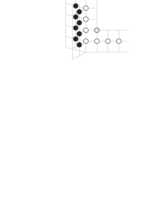
Figure 1: A graphical representation of the Y-system proposed in [10] for ABJM theory. Each circle in this infinite 3D lattice corresponds to a Y-function.

We denote the various Y-functions as in [13] – there are fermionic functions $Y_{\scalebox{0.67}{\begin{picture}(5.21,0.0)\put(-1.5,1.2){$\oplus$}\end{picture}}}$ and $Y_{\scalebox{0.67}{\begin{picture}(5.21,0.0)\put(-1.5,1.2){$\otimes$}\end{picture}}}$, bosonic functions $Y_{\scalebox{0.5}{\begin{picture}(7.27,0.3)\put(-1.7,2.65){$\bigcirc$}\end{picture}}_{n}}$ ($n=2,3,\dots$), pyramid functions $Y_{\scalebox{0.6}[0.7]{\begin{picture}(7.24,0.2)\put(-1.5,0.5){$\bigtriangleup$}\end{picture}}_{n}}$ ($n=2,3,\dots$) and middle node functions $Y_{{\scalebox{0.67}{\begin{picture}(5.21,0.0)\put(-1.5,1.2){$\blacktriangleright$}\end{picture}}}_{n}},Y_{{\scalebox{0.67}{\begin{picture}(5.21,0.0)\put(-1.5,1.2){$\blacktriangleleft$}\end{picture}}}_{n}}$ ($n=1,2,\dots$). As the state we consider belongs to the $sl(2)$ subsector of the theory, the middle node Y-functions of two types, corresponding to two series of black nodes in figure 1, are pairwise equal. We denote these Y-functions by $Y_{\scalebox{1.15}{\begin{picture}(2.8,0.0)\put(-1.2,-0.33){$\bullet$}\end{picture}}_{a}}$ or $Y_{a,0}$, so that we have $Y_{{\scalebox{0.67}{\begin{picture}(5.21,0.0)\put(-1.5,1.2){$\blacktriangleright$}\end{picture}}}_{a}}=Y_{{\scalebox{0.67}{\begin{picture}(5.21,0.0)\put(-1.5,1.2){$\blacktriangleleft$}\end{picture}}}_{a}}=Y_{\scalebox{1.15}{\begin{picture}(2.8,0.0)\put(-1.2,-0.33){$\bullet$}\end{picture}}_{a}}=Y_{a,0}$ for all $a$.

The TBA equations which describe the exact energy of the ground state in finite volume were proposed in [12], [13]. In [13] they were also extended via the contour deformation trick [37] to excited states in the $sl(2)$ subsector, the resulting equations being:

$$\log Y_{\scalebox{0.67}{\begin{picture}(5.21,0.0)\put(-1.5,1.2){$\otimes$}\end{picture}}} = +K_{m-1}*\log\frac{1+1/Y_{\scalebox{0.5}{\begin{picture}(7.27,0.3)\put(-1.7,2.65){$\bigcirc$}\end{picture}}_{m}}}{1+Y_{\scalebox{0.6}[0.7]{\begin{picture}(7.24,0.2)\put(-1.5,0.5){$\bigtriangleup$}\end{picture}}_{m}}}+2\mathcal{R}_{1m}^{(01)}*\log(1+Y_{\scalebox{1.15}{\begin{picture}(2.8,0.0)\put(-1.2,-0.33){$\bullet$}\end{picture}}_{m}})+2\left[\log\frac{R_{4}^{(+)}}{{R_{4}^{(-)}}}\right]+i\pi$$ (3.1)

$$\log Y_{\scalebox{0.67}{\begin{picture}(5.21,0.0)\put(-1.5,1.2){$\oplus$}\end{picture}}} = -K_{m-1}*\log\frac{1+1/Y_{\scalebox{0.5}{\begin{picture}(7.27,0.3)\put(-1.7,2.65){$\bigcirc$}\end{picture}}_{m}}}{1+Y_{\scalebox{0.6}[0.7]{\begin{picture}(7.24,0.2)\put(-1.5,0.5){$\bigtriangleup$}\end{picture}}_{m}}}-2\mathcal{B}_{1m}^{(01)}*\log(1+Y_{\scalebox{1.15}{\begin{picture}(2.8,0.0)\put(-1.2,-0.33){$\bullet$}\end{picture}}_{m}})-2\left[\log\frac{B_{4}^{(+)}}{{B_{4}^{(-)}}}\right]-i\pi$$ (3.2)

$$\log Y_{{\scalebox{0.6}[0.7]{\begin{picture}(7.24,0.2)\put(-1.5,0.5){$\bigtriangleup$}\end{picture}}}_{n}} = -K_{n-1,m-1}*\log(1+Y_{{\scalebox{0.6}[0.7]{\begin{picture}(7.24,0.2)\put(-1.5,0.5){$\bigtriangleup$}\end{picture}}}_{m}})-K_{n-1}*\log\frac{1+Y_{\scalebox{0.67}{\begin{picture}(5.21,0.0)\put(-1.5,1.2){$\otimes$}\end{picture}}}}{1+1/Y_{\scalebox{0.67}{\begin{picture}(5.21,0.0)\put(-1.5,1.2){$\oplus$}\end{picture}}}}$$

$$+ 2\left({\cal R}^{(01)}_{nm}+{\cal B}^{(01)}_{n-2,m}\right)*\log(1+Y_{\scalebox{1.15}{\begin{picture}(2.8,0.0)\put(-1.2,-0.33){$\bullet$}\end{picture}}_{m}})$$

$$+ 2\left[\sum\limits_{k=-\frac{n-1}{2}}^{\frac{n-1}{2}}\log\frac{R_{4}^{(+)}(u+ik)}{{R_{4}^{(-)}(u+ik)}}\right]+2\left[\sum\limits_{k=-\frac{n-3}{2}}^{\frac{n-3}{2}}\log\frac{B_{4}^{(+)}(u+ik)}{{B_{4}^{(-)}(u+ik)}}\right]$$

$$\log Y_{{\scalebox{0.5}{\begin{picture}(7.27,0.3)\put(-1.7,2.65){$\bigcirc$}\end{picture}}}_{n}} = K_{n-1,m-1}*\log(1+1/Y_{{\scalebox{0.5}{\begin{picture}(7.27,0.3)\put(-1.7,2.65){$\bigcirc$}\end{picture}}}_{m}})+K_{n-1}*\log\frac{1+Y_{\scalebox{0.67}{\begin{picture}(5.21,0.0)\put(-1.5,1.2){$\otimes$}\end{picture}}}}{1+1/Y_{\scalebox{0.67}{\begin{picture}(5.21,0.0)\put(-1.5,1.2){$\oplus$}\end{picture}}}}$$ (3.4)

$$\log Y_{{\scalebox{1.15}{\begin{picture}(2.8,0.0)\put(-1.2,-0.33){$\bullet$}\end{picture}}}_{n}} = (L+K_{4})\log\frac{x^{[-n]}}{x^{[+n]}}-{\cal B}_{n1}^{(10)}*\log(1+1/Y_{\scalebox{0.67}{\begin{picture}(5.21,0.0)\put(-1.5,1.2){$\oplus$}\end{picture}}})+{\cal R}_{n1}^{(10)}*\log(1+Y_{\scalebox{0.67}{\begin{picture}(5.21,0.0)\put(-1.5,1.2){$\otimes$}\end{picture}}})$$

$$+ \left({\cal R}_{nm}^{(10)}+{\cal B}_{n,m-2}^{(10)}\right)*\log(1+Y_{\scalebox{0.6}[0.7]{\begin{picture}(7.24,0.2)\put(-1.5,0.5){$\bigtriangleup$}\end{picture}}_{m}})$$

$$+ \left(2\tilde{\cal S}_{nm}-{\cal R}_{nm}^{(11)}+{\cal B}_{nm}^{(11)}\right)*\log(1+Y_{\scalebox{1.15}{\begin{picture}(2.8,0.0)\put(-1.2,-0.33){$\bullet$}\end{picture}}_{m}})+\left[\sum_{k=-\frac{n-1}{2}}^{\frac{n-1}{2}}\log\Phi(u+ik)\right]+i\pi n$$

Here and throughout the paper we use notation that is given in Appendix A. We also assume summation over the repeated index $m$.

The exact Bethe roots $u_{4,j}=u_{\bar{4},j}$ are fixed by the exact Bethe equations,

$$Y_{\scalebox{1.15}{\begin{picture}(2.8,0.0)\put(-1.2,-0.33){$\bullet$}\end{picture}}_{1}}^{\rm ph}(u_{4,j})=-1,\ \ \ \ j=1,2,\dots,K_{4}$$ (3.6)

and in general the values of these Bethe roots may differ from those one gets from the ABA. In the case we are studying the roots remain at zero within our precision – we have checked this numerically, verifying (3.6) with the use of equation (3) which we analytically continued as in [16].

The energy of the state we are studying is written in terms of the Y-functions as

$$E=E_{ABA}+\delta E,\ \ \ \delta E=2\sum_{a=1}^{\infty}\int_{-\infty}^{\infty}\frac{du}{2\pi i}\frac{\partial\epsilon_{a}^{{\rm mir}}(u)}{\partial u}\log(1+Y^{{\rm mir}}_{\scalebox{1.15}{\begin{picture}(2.8,0.0)\put(-1.2,-0.33){$\bullet$}\end{picture}}_{a}})$$ (3.7)

where $\epsilon_{a}(u)$ is defined by (2.10).

As our goal is to solve the TBA equations numerically, we will make to them several modifications, which are described below.

First, we substract from the original equations the equations which are satisfied by the asymptotic large $L$ solution of the Y-system [10], [13]. Let us describe this solution for the state discussed in section 2 which belongs to the $sl(2)$ subsector and has $L=1$, $K_{4}=K_{\bar{4}}=1$ with two Bethe roots $u_{4}=u_{\bar{4}}=0$. We use bold font to denote the asymptotic Y- and T-functions. The main formulas are:

$${\bf Y}_{\scalebox{0.6}[0.7]{\begin{picture}(7.24,0.2)\put(-1.5,0.5){$\bigtriangleup$}\end{picture}}_{a}}=\frac{{\bf T}^{+}_{a,1}{\bf T}^{-}_{a,1}}{{\bf T}_{a+1,1}{\bf T}_{a-1,1}}-1\;\;,\;\;1/{\bf Y}_{\scalebox{0.5}{\begin{picture}(7.27,0.3)\put(-1.7,2.65){$\bigcirc$}\end{picture}}_{s}}=\frac{{\bf T}^{+}_{1,s}{\bf T}^{-}_{1,s}}{{\bf T}_{1,s+1}{\bf T}_{1,s-1}}-1$$ (3.8)

$${\bf Y}_{\scalebox{0.67}{\begin{picture}(5.21,0.0)\put(-1.5,1.2){$\oplus$}\end{picture}}}=\frac{{\bf T}_{2,3}{\bf T}_{2,1}}{{\bf T}_{3,2}{\bf T}_{1,2}},\ {\bf Y}_{\scalebox{0.67}{\begin{picture}(5.21,0.0)\put(-1.5,1.2){$\otimes$}\end{picture}}}=\frac{{\bf T}_{1,2}{\bf T}_{1,0}}{{\bf T}_{2,1}{\bf T}_{0,1}}.\$$ (3.9)

All the ${\bf T}_{a,s}$ functions can be found from the generating functional ${\cal W}$. In particular

$${\cal W}=\sum_{s=0}^{\infty}{\bf T}_{1,s}(u+i\tfrac{1-s}{2})D^{s}\;\;,\;\;{\cal W}^{-1}=\sum_{a=0}^{\infty}(-1)^{a}{\bf T}_{a,1}(u+i\tfrac{1-a}{2})D^{a}\;.$$ (3.10)

$${\cal W} = \left(1-\left(\frac{B_{4}^{(+)+}}{B_{4}^{(-)+}}\frac{R_{4}^{(+)-}}{R_{4}^{(-)-}}\right)^{2}D\right)\left(1-\left(\frac{R_{4}^{(+)-}}{R_{4}^{(-)-}}\right)^{2}\,D\right)^{-1}$$ (3.11)

$$\times \left(1-\left(\frac{R_{4}^{(+)-}}{R_{4}^{(-)-}}\right)^{2}\,D\right)^{-1}\left(1-D\right)$$

where $D=e^{-i\partial_{u}}$. Finally,

$${\bf Y}_{\scalebox{1.15}{\begin{picture}(2.8,0.0)\put(-1.2,-0.33){$\bullet$}\end{picture}}_{a}}(u)=\left(\frac{x^{[-a]}}{x^{[+a]}}\right)^{L}\Phi_{a}(u){\bf T}_{a,1}(u).$$ (3.12)

A remarkable property of these asymptotic Y-functions is that they satisfy a set of TBA-type equations. This is true not only for $\lambda\to 0$, but also for finite values of $\lambda$ and $L$ (see e.g. [20], [38]). The equations satisfied by the asymptotic solution are the same as the original TBA equations given above, except that the terms in the r.h.s. which involve the $Y_{\scalebox{1.15}{\begin{picture}(2.8,0.0)\put(-1.2,-0.33){$\bullet$}\end{picture}}_{n}}$-functions should be omitted. After substracting these equations from the original ones and also slightly rewriting the kernels for more convenient numerics (similarly to [16]) we get:

$$\log\frac{Y_{\scalebox{0.67}{\begin{picture}(5.21,0.0)\put(-1.5,1.2){$\otimes$}\end{picture}}}}{{\bf Y_{\scalebox{0.67}{\begin{picture}(5.21,0.0)\put(-1.5,1.2){$\otimes$}\end{picture}}}}} = +K_{m-1}*\log\frac{1+1/Y_{\scalebox{0.5}{\begin{picture}(7.27,0.3)\put(-1.7,2.65){$\bigcirc$}\end{picture}}_{m}}}{1+Y_{\scalebox{0.6}[0.7]{\begin{picture}(7.24,0.2)\put(-1.5,0.5){$\bigtriangleup$}\end{picture}}_{m}}}\frac{1+{\bf Y}_{\scalebox{0.6}[0.7]{\begin{picture}(7.24,0.2)\put(-1.5,0.5){$\bigtriangleup$}\end{picture}}_{m}}}{1+1/{\bf Y}_{\scalebox{0.5}{\begin{picture}(7.27,0.3)\put(-1.7,2.65){$\bigcirc$}\end{picture}}_{m}}}+2\mathcal{R}^{(0m)}*\log(1+Y_{\scalebox{1.15}{\begin{picture}(2.8,0.0)\put(-1.2,-0.33){$\bullet$}\end{picture}}_{m}})$$ (3.13)

$$\log\frac{Y_{\scalebox{0.67}{\begin{picture}(5.21,0.0)\put(-1.5,1.2){$\oplus$}\end{picture}}}}{{\bf Y}_{\scalebox{0.67}{\begin{picture}(5.21,0.0)\put(-1.5,1.2){$\oplus$}\end{picture}}}} = -K_{m-1}*\log\frac{1+1/Y_{\scalebox{0.5}{\begin{picture}(7.27,0.3)\put(-1.7,2.65){$\bigcirc$}\end{picture}}_{m}}}{1+Y_{\scalebox{0.6}[0.7]{\begin{picture}(7.24,0.2)\put(-1.5,0.5){$\bigtriangleup$}\end{picture}}_{m}}}\frac{1+{\bf Y}_{\scalebox{0.6}[0.7]{\begin{picture}(7.24,0.2)\put(-1.5,0.5){$\bigtriangleup$}\end{picture}}_{m}}}{1+1/{\bf Y}_{\scalebox{0.5}{\begin{picture}(7.27,0.3)\put(-1.7,2.65){$\bigcirc$}\end{picture}}_{m}}}-2\mathcal{B}^{(0m)}*\log(1+Y_{\scalebox{1.15}{\begin{picture}(2.8,0.0)\put(-1.2,-0.33){$\bullet$}\end{picture}}_{m}})$$ (3.14)

$$\log\frac{Y_{{\scalebox{0.6}[0.7]{\begin{picture}(7.24,0.2)\put(-1.5,0.5){$\bigtriangleup$}\end{picture}}}_{n}}}{{\bf Y}_{{\scalebox{0.6}[0.7]{\begin{picture}(7.24,0.2)\put(-1.5,0.5){$\bigtriangleup$}\end{picture}}}_{n}}} = -K_{n-1,m-1}*\log\frac{(1+Y_{{\scalebox{0.6}[0.7]{\begin{picture}(7.24,0.2)\put(-1.5,0.5){$\bigtriangleup$}\end{picture}}}_{m}})}{(1+{\bf Y}_{{\scalebox{0.6}[0.7]{\begin{picture}(7.24,0.2)\put(-1.5,0.5){$\bigtriangleup$}\end{picture}}}_{m}})}-K_{n-1}*\log\frac{1+Y_{\scalebox{0.67}{\begin{picture}(5.21,0.0)\put(-1.5,1.2){$\otimes$}\end{picture}}}}{1+1/Y_{\scalebox{0.67}{\begin{picture}(5.21,0.0)\put(-1.5,1.2){$\oplus$}\end{picture}}}}\frac{1+1/{\bf Y}_{\scalebox{0.67}{\begin{picture}(5.21,0.0)\put(-1.5,1.2){$\oplus$}\end{picture}}}}{1+{\bf Y}_{\scalebox{0.67}{\begin{picture}(5.21,0.0)\put(-1.5,1.2){$\otimes$}\end{picture}}}}$$

$$+ 2{\cal M}_{nm}*\log(1+Y_{\scalebox{1.15}{\begin{picture}(2.8,0.0)\put(-1.2,-0.33){$\bullet$}\end{picture}}_{m}})$$

$$\log\frac{Y_{{\scalebox{0.5}{\begin{picture}(7.27,0.3)\put(-1.7,2.65){$\bigcirc$}\end{picture}}}_{n}}}{{\bf Y}_{{\scalebox{0.5}{\begin{picture}(7.27,0.3)\put(-1.7,2.65){$\bigcirc$}\end{picture}}}_{n}}} = K_{n-1,m-1}*\log\frac{(1+1/Y_{{\scalebox{0.5}{\begin{picture}(7.27,0.3)\put(-1.7,2.65){$\bigcirc$}\end{picture}}}_{m}})}{(1+1/{\bf Y}_{{\scalebox{0.5}{\begin{picture}(7.27,0.3)\put(-1.7,2.65){$\bigcirc$}\end{picture}}}_{m}})}+K_{n-1}*\log\frac{1+Y_{\scalebox{0.67}{\begin{picture}(5.21,0.0)\put(-1.5,1.2){$\otimes$}\end{picture}}}}{1+1/Y_{\scalebox{0.67}{\begin{picture}(5.21,0.0)\put(-1.5,1.2){$\oplus$}\end{picture}}}}\frac{1+1/{\bf Y}_{\scalebox{0.67}{\begin{picture}(5.21,0.0)\put(-1.5,1.2){$\oplus$}\end{picture}}}}{1+{\bf Y}_{\scalebox{0.67}{\begin{picture}(5.21,0.0)\put(-1.5,1.2){$\otimes$}\end{picture}}}}$$ (3.16)

$$\log\frac{Y_{{\scalebox{1.15}{\begin{picture}(2.8,0.0)\put(-1.2,-0.33){$\bullet$}\end{picture}}}_{n}}}{{\bf Y}_{{\scalebox{1.15}{\begin{picture}(2.8,0.0)\put(-1.2,-0.33){$\bullet$}\end{picture}}}_{n}}} = -{\cal B}^{(n0)}*\log\frac{(1+1/Y_{\scalebox{0.67}{\begin{picture}(5.21,0.0)\put(-1.5,1.2){$\oplus$}\end{picture}}})}{(1+1/{\bf Y}_{\scalebox{0.67}{\begin{picture}(5.21,0.0)\put(-1.5,1.2){$\oplus$}\end{picture}}})}+{\cal R}^{(n0)}*\log\frac{(1+Y_{\scalebox{0.67}{\begin{picture}(5.21,0.0)\put(-1.5,1.2){$\otimes$}\end{picture}}})}{(1+{\bf Y}_{\scalebox{0.67}{\begin{picture}(5.21,0.0)\put(-1.5,1.2){$\otimes$}\end{picture}}})}$$

$$+ {\cal N}_{nm}*\log\frac{(1+Y_{\scalebox{0.6}[0.7]{\begin{picture}(7.24,0.2)\put(-1.5,0.5){$\bigtriangleup$}\end{picture}}_{m}})}{(1+{\bf Y}_{\scalebox{0.6}[0.7]{\begin{picture}(7.24,0.2)\put(-1.5,0.5){$\bigtriangleup$}\end{picture}}_{m}})}$$

$$+ \left(2\tilde{\cal S}_{nm}-{\cal R}_{nm}^{(11)}+{\cal B}_{nm}^{(11)}\right)*\log(1+Y_{\scalebox{1.15}{\begin{picture}(2.8,0.0)\put(-1.2,-0.33){$\bullet$}\end{picture}}_{m}})$$

Note that in the Konishi case the function $Y_{\scalebox{0.6}[0.7]{\begin{picture}(7.24,0.2)\put(-1.5,0.5){$\bigtriangleup$}\end{picture}}_{2}}(u)$ had poles at the positions of the Bethe roots; in accordance with that, in our case it has a double pole at $u=0$. The asymptotic Y-function ${\bf Y}_{\scalebox{0.6}[0.7]{\begin{picture}(7.24,0.2)\put(-1.5,0.5){$\bigtriangleup$}\end{picture}}_{2}}(u)$ also has a double pole at $u=0$, so the combination $\frac{1+{Y}_{\scalebox{0.6}[0.7]{\begin{picture}(7.24,0.2)\put(-1.5,0.5){$\bigtriangleup$}\end{picture}}_{2}}(u)}{1+{\bf Y}_{\scalebox{0.6}[0.7]{\begin{picture}(7.24,0.2)\put(-1.5,0.5){$\bigtriangleup$}\end{picture}}_{2}}(u)}$ which appears in the equations (3.13)–(3) has no singularities on the real axis.

In the next section we discuss a further simplification to these equations which leaves only a finite number of unknown functions.

4 Truncating the TBA equations

The truncation method which we describe in this section has been proposed in [24] and is a simpler version of the general treatment in [20]. Unlike the method of [20] it involves some approximations, and it also relies on certain analyticity assumptions for the Y-functions. We will not discuss these assumptions here, but we have confirmed numerically that in our case the resulting equations are consistent with the original TBA of [13].

The truncation is done as follows. First, remarkably, it is possible to eliminate all the $Y_{\scalebox{0.5}{\begin{picture}(7.27,0.3)\put(-1.7,2.65){$\bigcirc$}\end{picture}}_{n}}$ functions from the TBA equations, replacing them by a single unknown function. The reason is that the Y-system equations for these functions are quite simple,

$${Y_{{\scalebox{0.5}{\begin{picture}(7.27,0.3)\put(-1.7,2.65){$\bigcirc$}\end{picture}}}_{n}}^{+}Y_{{\scalebox{0.5}{\begin{picture}(7.27,0.3)\put(-1.7,2.65){$\bigcirc$}\end{picture}}}_{n}}^{-}}=(1+Y_{{\scalebox{0.5}{\begin{picture}(7.27,0.3)\put(-1.7,2.65){$\bigcirc$}\end{picture}}}_{n+1}})(1+Y_{{\scalebox{0.5}{\begin{picture}(7.27,0.3)\put(-1.7,2.65){$\bigcirc$}\end{picture}}}_{n-1}})\,\,,\,\,n\geq 3$$ (4.1)

and to solve them we can use the following ansatz for the corresponding T-functions (see [39], [24], [20]):

$$T_{1,s}=s+K_{s}*f_{R}$$ (4.2)

where $f_{R}$ is a new unknown function. The $Y_{\scalebox{0.5}{\begin{picture}(7.27,0.3)\put(-1.7,2.65){$\bigcirc$}\end{picture}}_{n}}$ functions are obtained [10], [13], as usual, from

$${Y}_{\scalebox{0.5}{\begin{picture}(7.27,0.3)\put(-1.7,2.65){$\bigcirc$}\end{picture}}_{n}}=\left(\frac{{T}^{+}_{1,n}{T}^{-}_{1,n}}{{T}_{1,n+1}{T}_{1,n-1}}-1\right)^{-1},$$ (4.3)

and it can be shown that the infinite set of equations (4.1) is indeed satisfied for any $f_{R}$ with suitable analyticity properties. This function is fixed by the TBA equations – the infinite set of equations (3.16) reduces to a single equation for $f_{R}$. That equation has the form

$$\frac{1+Y_{\scalebox{0.67}{\begin{picture}(5.21,0.0)\put(-1.5,1.2){$\otimes$}\end{picture}}}}{1+1/Y_{\scalebox{0.67}{\begin{picture}(5.21,0.0)\put(-1.5,1.2){$\oplus$}\end{picture}}}}=\frac{\left(1+K_{1}^{+}*_{p.v.}f_{R}+f_{R}/2\right)\left(1+K_{1}^{-}*_{p.v.}f_{R}+f_{R}/2\right)}{\left(1+K_{1}^{+}*_{p.v.}f_{R}-f_{R}/2\right)\left(1+K_{1}^{-}*_{p.v.}f_{R}-f_{R}/2\right)}$$ (4.4)

where $*_{p.v.}$ denotes principal value integration. Solving for $f_{R}$ we get an expression suitable for numerical iterations:

$$f_{R}=2\frac{(a+1)(y+1)-\sqrt{4(a+1)^{2}y^{2}-b^{2}(y-1)^{2}}}{y-1}$$ (4.5)

where $y=\frac{1+Y_{\scalebox{0.67}{\begin{picture}(5.21,0.0)\put(-1.5,1.2){$\otimes$}\end{picture}}}}{1+1/Y_{\scalebox{0.67}{\begin{picture}(5.21,0.0)\put(-1.5,1.2){$\oplus$}\end{picture}}}},\ a={\rm Re}\left(K_{1}^{+}*_{p.v.}f_{R}\right),\ b={\rm Im}\left(K_{1}^{+}*_{p.v.}f_{R}\right)$.

Note that the Y-system equation for $Y_{\scalebox{0.5}{\begin{picture}(7.27,0.3)\put(-1.7,2.65){$\bigcirc$}\end{picture}}_{2}}$, which reads

$${Y_{{\scalebox{0.5}{\begin{picture}(7.27,0.3)\put(-1.7,2.65){$\bigcirc$}\end{picture}}}_{2}}^{+}Y_{{\scalebox{0.5}{\begin{picture}(7.27,0.3)\put(-1.7,2.65){$\bigcirc$}\end{picture}}}_{2}}^{-}}=\frac{(1+Y_{\scalebox{0.67}{\begin{picture}(5.21,0.0)\put(-1.5,1.2){$\otimes$}\end{picture}}})(1+Y_{{\scalebox{0.5}{\begin{picture}(7.27,0.3)\put(-1.7,2.65){$\bigcirc$}\end{picture}}}_{3}})}{1+1/Y_{\scalebox{0.67}{\begin{picture}(5.21,0.0)\put(-1.5,1.2){$\oplus$}\end{picture}}}},$$ (4.6)

is not satisfied automatically for arbitrary $f_{R}$ (since it includes the fermionic functions $Y_{\scalebox{0.67}{\begin{picture}(5.21,0.0)\put(-1.5,1.2){$\oplus$}\end{picture}}},Y_{\scalebox{0.67}{\begin{picture}(5.21,0.0)\put(-1.5,1.2){$\otimes$}\end{picture}}}$), but will hold provided that the TBA equations are satisfied.

So far we haven’t made any approximations in the TBA equations – the truncation we have just described is exact. However, we cannot directly apply the same method in the upper wing of the Y-system to replace the functions $Y_{\scalebox{0.6}[0.7]{\begin{picture}(7.24,0.2)\put(-1.5,0.5){$\bigtriangleup$}\end{picture}}_{n}},Y_{\scalebox{1.15}{\begin{picture}(2.8,0.0)\put(-1.2,-0.33){$\bullet$}\end{picture}}_{n}}$ by a finite number of unknown ones, as the Y-system equations for $Y_{\scalebox{0.6}[0.7]{\begin{picture}(7.24,0.2)\put(-1.5,0.5){$\bigtriangleup$}\end{picture}}_{n}},Y_{\scalebox{1.15}{\begin{picture}(2.8,0.0)\put(-1.2,-0.33){$\bullet$}\end{picture}}_{n}}$ are more complicated than (4.1). But since the $Y_{\scalebox{1.15}{\begin{picture}(2.8,0.0)\put(-1.2,-0.33){$\bullet$}\end{picture}}_{n}}$ functions decay fast with $n$, within our precision it is enough to keep only the first 6 or 7 of them and set the other ones to zero. With this approximation we see that for $n>M$, where $M$ the number of $Y_{\scalebox{1.15}{\begin{picture}(2.8,0.0)\put(-1.2,-0.33){$\bullet$}\end{picture}}_{n}}$ functions that we retain, the pyramid Y-functions $Y_{\scalebox{0.6}[0.7]{\begin{picture}(7.24,0.2)\put(-1.5,0.5){$\bigtriangleup$}\end{picture}}_{n}}$ decouple from the rest of the Y-system and are governed by an equation very similar to (4.1):

$${Y_{{\scalebox{0.6}[0.7]{\begin{picture}(7.24,0.2)\put(-1.5,0.5){$\bigtriangleup$}\end{picture}}}_{n}}^{+}Y_{{\scalebox{0.6}[0.7]{\begin{picture}(7.24,0.2)\put(-1.5,0.5){$\bigtriangleup$}\end{picture}}}_{n}}^{-}}=\frac{1}{(1+1/Y_{{\scalebox{0.6}[0.7]{\begin{picture}(7.24,0.2)\put(-1.5,0.5){$\bigtriangleup$}\end{picture}}}_{n+1}})(1+1/Y_{{\scalebox{0.6}[0.7]{\begin{picture}(7.24,0.2)\put(-1.5,0.5){$\bigtriangleup$}\end{picture}}}_{n-1}})}\,\,,\,\,n>M.$$ (4.7)

This equation is solved by an ansatz analogous to (4.2):

$$T_{a,1}=a+K_{a-M+1}*f_{U}$$ (4.8)

with ${Y}_{\scalebox{0.6}[0.7]{\begin{picture}(7.24,0.2)\put(-1.5,0.5){$\bigtriangleup$}\end{picture}}_{a}}=\frac{{T}^{+}_{a,1}{T}^{-}_{a,1}}{{T}_{a+1,1}{T}_{a-1,1}}-1$. Here $f_{U}$ is another new unknown function, and it is fixed by an equation similar to (4.5):

$$f_{U}=a(4y-2)-2(\sqrt{(y-1)y(2a+M+1)^{2}-b^{2}}-(M+1)y+M)$$ (4.9)

where $y=1+Y_{\scalebox{0.6}[0.7]{\begin{picture}(7.24,0.2)\put(-1.5,0.5){$\bigtriangleup$}\end{picture}}_{M}},\ a={\rm Re}\left(K_{1}^{+}*_{p.v.}f_{U}\right),\ b={\rm Im}\left(K_{1}^{+}*_{p.v.}f_{U}\right)$.

Lastly, we need to rewrite the r.h.s. of the remaining TBA equations in terms of the new functions $f_{R},f_{U}$. To do this, we will need the exact T-functions – which are given by (4.2), (4.8) – and the asymptotic T-functions, which are obtained from the same expressions when $f_{R},f_{U}$ are replaced by ${{\bf f}_{R}},{{\bf f}_{U}}$:

$${{\bf f}_{R}}(u)=\frac{x^{{\rm mir}}(u-i0)-1/x^{{\rm mir}}(u+i0)}{x_{4}^{{\rm mir}+}-1/x_{4}^{{\rm mir}-}},\ \ {{\bf f}_{U}}(u)=K_{M-1}(u,v)*\frac{x^{{\rm mir}}(v-i0)-1/x^{{\rm mir}}(v+i0)}{\left(1/x_{4}^{{\rm mir}+}\right)-x_{4}^{{\rm mir}-}}.$$ (4.10)

We list the remaining TBA equations below.

Equations for fermions:

$$\log\frac{Y_{\scalebox{0.67}{\begin{picture}(5.21,0.0)\put(-1.5,1.2){$\otimes$}\end{picture}}}}{{\bf Y}_{\scalebox{0.67}{\begin{picture}(5.21,0.0)\put(-1.5,1.2){$\otimes$}\end{picture}}}} = \log\frac{T_{1,2}}{{\bf T}_{1,2}}-K_{1}*\log\frac{T_{1,1}}{{\bf T}_{1,1}}-K_{M-1}*\log\frac{T_{M+1,1}}{{\bf T}_{M+1,1}}+K_{M}*\log\frac{T_{M,1}}{{\bf T}_{M,1}}$$

$$- \sum_{m=2}^{M}K_{m-1}*\log\frac{1+Y_{\scalebox{0.6}[0.7]{\begin{picture}(7.24,0.2)\put(-1.5,0.5){$\bigtriangleup$}\end{picture}}_{m}}}{1+{\bf Y}_{\scalebox{0.6}[0.7]{\begin{picture}(7.24,0.2)\put(-1.5,0.5){$\bigtriangleup$}\end{picture}}_{m}}}+2\mathcal{R}^{(0m)}*\log(1+Y_{\scalebox{1.15}{\begin{picture}(2.8,0.0)\put(-1.2,-0.33){$\bullet$}\end{picture}}_{m}})$$

$$\log\frac{Y_{\scalebox{0.67}{\begin{picture}(5.21,0.0)\put(-1.5,1.2){$\oplus$}\end{picture}}}}{{\bf Y}_{\scalebox{0.67}{\begin{picture}(5.21,0.0)\put(-1.5,1.2){$\oplus$}\end{picture}}}} = -\log\frac{T_{1,2}}{{\bf T}_{1,2}}+K_{1}*\log\frac{T_{1,1}}{{\bf T}_{1,1}}+K_{M-1}*\log\frac{T_{M+1,1}}{{\bf T}_{M+1,1}}-K_{M}*\log\frac{T_{M,1}}{{\bf T}_{M,1}}$$ (4.12)

$$+ \sum_{m=2}^{M}K_{m-1}*\log\frac{1+Y_{\scalebox{0.6}[0.7]{\begin{picture}(7.24,0.2)\put(-1.5,0.5){$\bigtriangleup$}\end{picture}}_{m}}}{1+{\bf Y}_{\scalebox{0.6}[0.7]{\begin{picture}(7.24,0.2)\put(-1.5,0.5){$\bigtriangleup$}\end{picture}}_{m}}}-2\mathcal{B}^{(0m)}*\log(1+Y_{\scalebox{1.15}{\begin{picture}(2.8,0.0)\put(-1.2,-0.33){$\bullet$}\end{picture}}_{m}}).$$

Equations for pyramids ($n=2,\dots,M$)

$$\log\frac{Y_{{\scalebox{0.6}[0.7]{\begin{picture}(7.24,0.2)\put(-1.5,0.5){$\bigtriangleup$}\end{picture}}}_{n}}}{{\bf Y}_{{\scalebox{0.6}[0.7]{\begin{picture}(7.24,0.2)\put(-1.5,0.5){$\bigtriangleup$}\end{picture}}}_{n}}} = -\delta_{n,M}\log\frac{T_{M+1,1}}{{\bf T}_{M+1,1}}-K_{n-1,M-1}*\log\frac{T_{M+1,1}}{{\bf T}_{M+1,1}}+K_{n-1,M}*\log\frac{T_{M,1}}{{\bf T}_{M,1}}$$

$$- \sum_{m=2}^{M}K_{n-1,m-1}*\log\frac{1+Y_{\scalebox{0.6}[0.7]{\begin{picture}(7.24,0.2)\put(-1.5,0.5){$\bigtriangleup$}\end{picture}}_{m}}}{1+{\bf Y}_{\scalebox{0.6}[0.7]{\begin{picture}(7.24,0.2)\put(-1.5,0.5){$\bigtriangleup$}\end{picture}}_{m}}}-K_{n-1}*\log\frac{1+Y_{\scalebox{0.67}{\begin{picture}(5.21,0.0)\put(-1.5,1.2){$\otimes$}\end{picture}}}}{1+1/Y_{\scalebox{0.67}{\begin{picture}(5.21,0.0)\put(-1.5,1.2){$\oplus$}\end{picture}}}}\frac{1+1/{\bf Y}_{\scalebox{0.67}{\begin{picture}(5.21,0.0)\put(-1.5,1.2){$\oplus$}\end{picture}}}}{1+{\bf Y}_{\scalebox{0.67}{\begin{picture}(5.21,0.0)\put(-1.5,1.2){$\otimes$}\end{picture}}}}$$

$$+ 2{\cal M}_{nm}*\log(1+Y_{\scalebox{1.15}{\begin{picture}(2.8,0.0)\put(-1.2,-0.33){$\bullet$}\end{picture}}_{m}}).$$

Equations for middle nodes ($n=1,2,\dots,M$):

$$\log\frac{Y_{{\scalebox{1.15}{\begin{picture}(2.8,0.0)\put(-1.2,-0.33){$\bullet$}\end{picture}}}_{n}}}{{\bf Y}_{{\scalebox{1.15}{\begin{picture}(2.8,0.0)\put(-1.2,-0.33){$\bullet$}\end{picture}}}_{n}}} = \left(2\tilde{\cal S}_{nm}-{\cal R}_{nm}^{(11)}+{\cal B}_{nm}^{(11)}\right)*\log(1+Y_{\scalebox{1.15}{\begin{picture}(2.8,0.0)\put(-1.2,-0.33){$\bullet$}\end{picture}}_{m}})$$

$$- {\cal B}^{(n0)}*\log\frac{(1+1/Y_{\scalebox{0.67}{\begin{picture}(5.21,0.0)\put(-1.5,1.2){$\oplus$}\end{picture}}})}{(1+1/{\bf Y}_{\scalebox{0.67}{\begin{picture}(5.21,0.0)\put(-1.5,1.2){$\oplus$}\end{picture}}})}+{\cal R}^{(n0)}*\log\frac{(1+Y_{\scalebox{0.67}{\begin{picture}(5.21,0.0)\put(-1.5,1.2){$\otimes$}\end{picture}}})}{(1+{\bf Y}_{\scalebox{0.67}{\begin{picture}(5.21,0.0)\put(-1.5,1.2){$\otimes$}\end{picture}}})}$$

$$+ \mathcal{R}^{(n0)}{\circlearrowright*\hskip 2.84526pt}\left(K_{M-1}*\log\frac{T_{M+1,1}}{{\bf T}_{M+1,1}}-K_{M}*\log\frac{T_{M,1}}{{\bf T}_{M,1}}+\sum_{m=2}^{M}K_{m-1}*\log\frac{1+Y_{\scalebox{0.6}[0.7]{\begin{picture}(7.24,0.2)\put(-1.5,0.5){$\bigtriangleup$}\end{picture}}_{m}}}{1+{\bf Y}_{\scalebox{0.6}[0.7]{\begin{picture}(7.24,0.2)\put(-1.5,0.5){$\bigtriangleup$}\end{picture}}_{m}}}\right)$$

$$+ K^{\neq}_{n-1,M-1}*\log\frac{T_{M+1,1}}{{\bf T}_{M+1,1}}-K^{\neq}_{n-1,M}*\log\frac{T_{M,1}}{{\bf T}_{M,1}}+\sum_{m=2}^{M}K^{\neq}_{n-1,m-1}*\log\frac{1+Y_{\scalebox{0.6}[0.7]{\begin{picture}(7.24,0.2)\put(-1.5,0.5){$\bigtriangleup$}\end{picture}}_{m}}}{1+{\bf Y}_{\scalebox{0.6}[0.7]{\begin{picture}(7.24,0.2)\put(-1.5,0.5){$\bigtriangleup$}\end{picture}}_{m}}}.$$

As a result, the equations that we are solving numerically are (4.5), (4.9) and (4)–(4).

5 Numerical results

Our numerical strategy is similar to [16], and we are solving the TBA equations (4.5), (4.9), (4)–(4) by iterations. We truncated the number of middle node Y-functions to $M=6$ or 7, and used cutoffs on the $u$ axis to make finite the range of integration in the convolutions. The range of coupling that we study is $0\leq h(\lambda)\leq 1$ (since the TBA equations are written in terms of $h(\lambda)$, we obtain the anomalous dimension as a function of $h(\lambda)$).

Table 1: Numerical values of the correction to the Bethe ansatz result for the energy, with uncertainty in the last digit.

$h(\lambda)$	$\delta E(\lambda)$	$h(\lambda)$	$\delta E(\lambda)$
0.00	0.0000	0.55	0.0703
0.10	0.0005	0.60	0.069
0.15	0.0023	0.65	0.059
0.20	0.0063	0.70	0.041
0.25	0.0129	0.75	0.014
0.30	0.0221	0.80	-0.025
0.35	0.0332	0.85	-0.072
0.40	0.0451	0.90	-0.126
0.45	0.0566	0.95	-0.188
0.50	0.0655	1.00	-0.254

Our main result is the correction $\delta E$ to the ABA value for the energy (see (2.12)) and it is shown in Fig. 2. The numerical values of this correction are also listed in table 1. We estimated their absolute precision as about $\pm 10^{-4}$ for $h(\lambda)\leq 0.55$ and $\pm 10^{-3}$ for $h(\lambda)>0.55$. In Figure 3 we plot the full energy, including the ABA part. As expected, at weak coupling our numerical results are completely consistent with the leading wrapping correction obtained analytically in [10], [22] (this is also seen in Figure 2). As the coupling is increased, our results gradually deviate more and more from that prediction.

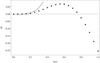
Figure 2: The correction $\delta E$ to the Bethe ansatz result for the energy, as a function of $h(\lambda)$, is shown by black dots. The solid line is the first wrapping correction given by (2.13).

The behaviour of middle-node Y-functions $Y_{\scalebox{1.15}{\begin{picture}(2.8,0.0)\put(-1.2,-0.33){$\bullet$}\end{picture}}_{n}}$ exhibits several interesting features. While in the AdS₅/CFT₄ Konishi case all these functions take positive values, here they have signs alternating with $n$, i.e. $Y_{\scalebox{1.15}{\begin{picture}(2.8,0.0)\put(-1.2,-0.33){$\bullet$}\end{picture}}_{1}}<0,\ Y_{\scalebox{1.15}{\begin{picture}(2.8,0.0)\put(-1.2,-0.33){$\bullet$}\end{picture}}_{2}}>0,\ Y_{\scalebox{1.15}{\begin{picture}(2.8,0.0)\put(-1.2,-0.33){$\bullet$}\end{picture}}_{3}}<0$ etc. In Figure 4 (left) we plot their absolute value for $h(\lambda)=0.9$. Since these Y-functions appear as $\log(1+Y_{\scalebox{1.15}{\begin{picture}(2.8,0.0)\put(-1.2,-0.33){$\bullet$}\end{picture}}_{n}})$ in the expression for the energy and in the TBA equations, their negative values beyond $-1$ would give rise to singularities. We discovered that as the coupling is increased, the middle-node Y-function $Y_{\scalebox{1.15}{\begin{picture}(2.8,0.0)\put(-1.2,-0.33){$\bullet$}\end{picture}}_{1}}$ indeed approaches the critical value $-1$ for $u$ close to zero (while other Y-functions remain far from this dangerous value). That is clearly seen from Figure 5 (left), and at $h(\lambda)=1$ we have $Y_{\scalebox{1.15}{\begin{picture}(2.8,0.0)\put(-1.2,-0.33){$\bullet$}\end{picture}}_{1}}(0)\approx-0.993$ which is already very close to the singularity. This means that proceeding further in the coupling would probably require obtaining $Y_{\scalebox{1.15}{\begin{picture}(2.8,0.0)\put(-1.2,-0.33){$\bullet$}\end{picture}}_{1}}$ with a high precision.

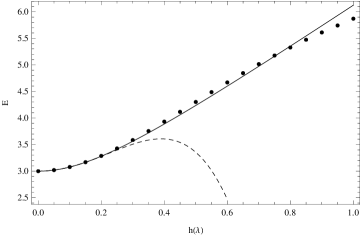
Figure 3: The full scaling dimension $E_{ABA}+\delta E$. Dots: numerics, solid line: ABA, dashed line: ABA + 1st wrapping as given by (2.14)

The corresponding asymptotic Y-function ${\bf Y}_{\scalebox{1.15}{\begin{picture}(2.8,0.0)\put(-1.2,-0.33){$\bullet$}\end{picture}}_{1}}$ already starts to take values beyond $-1$ at $h(\lambda)\approx 0.6$. However, that does not lead to any singularity since $\log(1+{\bf Y}_{\scalebox{1.15}{\begin{picture}(2.8,0.0)\put(-1.2,-0.33){$\bullet$}\end{picture}}_{1}})$ never appears in the TBA equations. In Figure 4 (right) we plot for comparison the exact and the asymptotic Y-function.

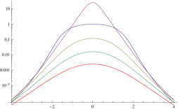
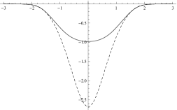
Figure 4: Left: The middle-node Y-functions $Y_{n,0}(u)$ for $h(\lambda)=0.9$. The figure shows plots of minus $Y_{1,0}$ (blue), $Y_{2,0}$ (purple), minus $Y_{3,0}$ (yellow), $Y_{4,0}$ (green) and minus $Y_{5,0}$ (red). Right: the exact Y-function $Y_{1,0}$ (solid line) and its asymptotic counterpart ${\bf Y}_{1,0}$ (dashed line) for $h(\lambda)=0.9$.

It is possible that if the coupling is increased further the function $Y_{\scalebox{1.15}{\begin{picture}(2.8,0.0)\put(-1.2,-0.33){$\bullet$}\end{picture}}_{1}}$ will cross the critical value $-1$. Then the TBA equations will probably require some modification such as extra driving terms, and it would be very interesting to understand whether this indeed happens for the state we are studying. For other models similar issues have been explored in [37], while in the AdS/CFT case the possibility of such singularities arising was discussed in e.g. [16], [41], [42].

The second middle-node Y-function $Y_{\scalebox{1.15}{\begin{picture}(2.8,0.0)\put(-1.2,-0.33){$\bullet$}\end{picture}}_{2}}$ also shows unusual behaviour, rapidly increasing in magnitude as the coupling is being increased. This is shown in Figure 5 (right).

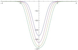
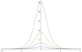
Figure 5: The middle-node Y-functions $Y_{1,0}(u)$ (left) and $Y_{2,0}(u)$ (right) for several values of the coupling: $h(\lambda)=0.6$ (blue), 0.7 (purple), 0.8 (yellow) and 0.9 (green).

Lastly, in Figure 6 we show the plots of the new functions $f_{R},f_{U}$ which parametrize the solution of the Y-system in the right wing and in the upper wing, respectively.

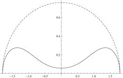
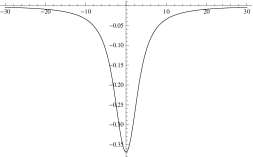
Figure 6: The functions $f_{R}(u)$ (left) and $f_{U}(u)$ (right) for $h(\lambda)=0.9$ and $M=7$, shown by solid lines. The dashed line in the left figure shows the asymptotic ${\bf f}_{R}$ function (4.10), while $f_{U}$ almost coincides with its asymptotic expression ${\bf f}_{U}$.

The total range of the coupling we have investigated, $0\leq h(\lambda)\leq 1$, is four times greater than the convergence radius $|h(\lambda)|\leq 0.25$ of the weak-coupling expansion of the ABA result (2.11), which suggests that we are exploring the intermediate coupling regime. We were not able to make a consistent prediction for the strong coupling expansion coefficients, but we hope this could be done in the future by going to greater values of the coupling. Increasing the coupling poses a challenge because beyond the value $h(\lambda)=1$ the iterative procedure we use for solving the TBA equations converges too slowly; hopefully this problem may be overcome by improving the numerical algorithm (e.g. using Newton’s method).

At strong coupling the leading term in the exact energy should be proportional to $\lambda^{1/4}$ [43] which in our case is equivalent to $\sqrt{h(\lambda)}$ (while string theory predictions for subleading terms are not available as of now). However, the strong-coupling behavior of the ABA result (2.11) is completely different

$$E_{ABA}=2\sqrt{2\lambda}+O(1)=4h(\lambda)+O(1),$$ (5.1)

suggesting that the leading asymptotics predicted by the ABA should cancel against the TBA correction $\delta E$. It is possible that we can already see this starting to happen for $h(\lambda)\geq 0.8$ when the exact energy becomes smaller than the ABA prediction. In Figure 7 we show a log-log plot of the full energy, and the ABA result asymptotes to a straight line, consistently with (5.1), while one may expect that the exact energy will asymptote to a straight line with a different slope.

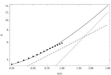
Figure 7: A log-log plot of the full conformal dimension $E$ vs. $h(\lambda)$. We show the ABA prediction (solid curve), its asymptote (dotted line defined by $E=4h(\lambda)$), our numerical data (black dots) and the expected slope of the result at strong coupling (dashed line defined by $E=\mbox{const}\times\sqrt{h(\lambda)}$).

6 Conclusions

In this paper we have applied the Thermodynamic Bethe ansatz approach to compute the exact anomalous dimension of a short operator in AdS₄/CFT₃, for the first time solving numerically the TBA equations for this theory. We have explored the values of the coupling $0\leq h(\lambda)\leq 1$ and at weak coupling our results are consistent with known predictions. We also found that as the coupling is being increased one of the Y-functions approaches the critical value $-1$. It would be very interesting to go to higher values of the coupling, and achieving that may be possible by improving the numerical strategy or perhaps by applying the very recent approach of [20]. Hopefully a comparison with string theory calculations could be made eventually at strong coupling, providing a deep test of the integrable structures in AdS₄/CFT₃ correspondence.

7 Appendix A: Notation

The R and B functions are

$$R_{a}^{(\pm)}=\prod_{j=1}^{K_{a}}\left[x(u)-x^{\mp}_{a,j}\right],\qquad B_{a}^{(\pm)}=\prod_{j=1}^{K_{a}}\left[\frac{1}{x(u)}-x^{\mp}_{a,j}\right],$$ (7.1)

where for the state we consider in this paper all $K_{a}$ are zero except $K_{4}=K_{\bar{4}}=1$. The scalar factor $\Phi$ is defined as

$$\Phi(u)=\frac{B_{4}^{(+)+}R_{4}^{(-)-}}{B_{4}^{(-)-}R_{4}^{(+)+}}\left(\prod_{j=1}^{K_{4}}\frac{x^{+}_{4,j}}{x^{-}_{4,j}}\right)\prod_{j=1}^{K_{4}}\sigma^{2}(u,u_{4,j}),\ \ \Phi_{a}(u)=\prod^{\frac{a-1}{2}}_{k=-\frac{a-1}{2}}\Phi(u+ik).$$ (7.2)

The kernels in TBA equations are:

$$K_{n}(u,v) \equiv \frac{1}{2\pi i}\frac{\partial}{\partial v}\ln\frac{u-v+in/2}{u-v-in/2}=\frac{2n/\pi}{n^{2}+4(u-v)^{2}},$$ (7.3)

$$K_{n,m}(u,v) \equiv \sum_{j=-\frac{m-1}{2}}^{\frac{m-1}{2}}\sum_{k=-\frac{n-1}{2}}^{\frac{n-1}{2}}K_{2j+2k+2}(u,v),$$ (7.4)

$$K_{n,m}^{\neq}(u,v) \equiv \sum_{j=-\frac{m-1}{2}}^{\frac{m-1}{2}}\sum_{k=-\frac{n-1}{2}}^{\frac{n-1}{2}}K_{2j+2k+1}(u,v),$$ (7.5)

where we assume $K_{0,n}=0,\ K_{0,n}^{\neq}=0$. Also,

$${\cal S}_{nm}(u,v) \equiv \frac{1}{2\pi i}\frac{\partial}{\partial v}\log\sigma_{BES}(x^{[+n]}(u),x^{[-n]}(u),x^{[+m]}(v),x^{[-m]}(v)),$$ (7.7)

$$\tilde{\cal S}_{nm}(u,v) \equiv {\cal S}_{nm}(u,v)+\frac{ni}{2}{\cal P}^{(m)}(v),$$ (7.8)

$$\mathcal{B}^{(ab)}_{nm}(u,v) \equiv \sum_{j=-\frac{n-1}{2}}^{\frac{n-1}{2}}\sum_{k=-\frac{m-1}{2}}^{\frac{m-1}{2}}\frac{1}{2\pi i}\frac{\partial}{\partial v}\log\frac{b(u+ia/2+ij,v-ib/2+ik)}{b(u-ia/2+ij,v+ib/2+ik)}$$ (7.9)

$$\mathcal{R}^{(ab)}_{nm}(u,v) \equiv \sum_{j=-\frac{n-1}{2}}^{\frac{n-1}{2}}\sum_{k=-\frac{m-1}{2}}^{\frac{m-1}{2}}\frac{1}{2\pi i}\frac{\partial}{\partial v}\log\frac{r(u+ia/2+ij,v-ib/2+ik)}{r(u-ia/2+ij,v+ib/2+ik)},$$ (7.10)

$${\cal R}^{(nm)}(u,v) \equiv \frac{\partial_{v}}{2\pi i}\log\frac{x_{u}^{[+n]}-x_{v}^{[-m]}}{x_{u}^{[-n]}-x_{v}^{[+m]}}-\frac{1}{2i}{\cal P}^{(m)}(v),$$ (7.11)

$${\cal B}^{(nm)}(u,v) \equiv \frac{\partial_{v}}{2\pi i}\log\frac{{1/x}_{u}^{[+n]}-x_{v}^{[-m]}}{{1/x}_{u}^{[-n]}-x_{v}^{[+m]}}-\frac{1}{2i}{\cal P}^{(m)}(v)$$ (7.12)

$${\cal M}_{nm} \equiv K_{n-1}{\circlearrowright*\hskip 2.84526pt}{\cal R}^{(0m)}+K^{\neq}_{n-1,m-1}\,,$$ (7.13)

$${\cal N}_{nm} \equiv {\cal R}^{(n0)}{\circlearrowright*\hskip 2.84526pt}K_{m-1}+K^{\neq}_{n-1,m-1}\,,$$ (7.14)

where

$$b(u,v)=\frac{1/x^{{\rm mir}}(u)-x^{{\rm mir}}(v)}{\sqrt{x^{{\rm mir}}(v)}},\ \ r(u,v)=\frac{x^{{\rm mir}}(u)-x^{{\rm mir}}(v)}{\sqrt{x^{{\rm mir}}(v)}},$$ (7.15)

and

$${\cal P}^{(a)}(v)=-\frac{1}{2\pi}\partial_{v}\log\frac{x^{{\rm mir}}(v+ia/2)}{x^{{\rm mir}}(v-ia/2)}\;.$$ (7.16)

The convolutions in integral equations are over the second variable, and $*$ denotes standard convolution along the real axis: $K(u,v)*f(v)\equiv\int^{+\infty}_{-\infty}dvK(u,v)f(v)$.

The symbol ${\circlearrowright*\hskip 2.84526pt}$ denotes convolution along with analytical continuation across the cut $u\in(-\infty,-2h)\cup(2h,+\infty)$ (see [13], [16]). E.g.

$${\cal R}^{(n0)}{\circlearrowright*\hskip 0.56905pt}\log(1+Y_{\scalebox{0.67}{\begin{picture}(5.21,0.0)\put(-1.5,1.2){$\otimes$}\end{picture}}})=\int_{-2h}^{2h}dv\left[{\cal R}^{(n0)}\log(1+Y_{\scalebox{0.67}{\begin{picture}(5.21,0.0)\put(-1.5,1.2){$\otimes$}\end{picture}}})-{\cal B}^{(n0)}\log(1+1/Y_{\scalebox{0.67}{\begin{picture}(5.21,0.0)\put(-1.5,1.2){$\oplus$}\end{picture}}})\right].$$ (7.17)

One should also be careful about which branch of $x(u)$ to use in various places in TBA equations. The mirror branch is used when $u$ is the free variable or the variable that is being integrated over. Otherwise the physical branch is used.

References

[1]
N. Beisert, C. Ahn, L. F. Alday, Z. Bajnok, J. M. Drummond, L. Freyhult, N. Gromov, R. A. Janik et al.,
“Review of AdS/CFT Integrability: An Overview,”
[arXiv:1012.3982 [hep-th]].
[2]
A. Babichenko, B. Stefanski, Jr., K. Zarembo,
“Integrability and the AdS(3)/CFT(2) correspondence,”
JHEP 1003 (2010) 058.
[arXiv:0912.1723 [hep-th]].
K. Zoubos,
“Review of AdS/CFT Integrability, Chapter IV.2: Deformations, Orbifolds and Open Boundaries,”
[arXiv:1012.3998 [hep-th]].
[3]
T. Klose,
“Review of AdS/CFT Integrability, Chapter IV.3: N=6 Chern-Simons and Strings on AdS4xCP3,”
[arXiv:1012.3999 [hep-th]].
[4]
O. Aharony, O. Bergman, D. L. Jafferis and J. Maldacena,
“N=6 superconformal Chern-Simons-matter theories, M2-branes and their
gravity duals”,
JHEP 0810, 091 (2008)
[arXiv:0806.1218 [hep-th]]
O. Aharony, O. Bergman and D. L. Jafferis,
“Fractional M2-branes”,
JHEP 0811, 043 (2008)
[arXiv:0807.4924 [hep-th]].
[5]
J. A. Minahan and K. Zarembo,
“The Bethe ansatz for superconformal Chern-Simons,”
JHEP 0809 (2008) 040
[arXiv:0806.3951 [hep-th]].
[6]
N. Gromov, P. Vieira,
“The all loop AdS4/CFT3 Bethe ansatz,”
JHEP 0901 (2009) 016.
[arXiv:0807.0777 [hep-th]].
[7]
C. Ahn and R.I. Nepomechie,
super Chern-Simons theory -matrix and all-loop Bethe ansatz
equations,
JHEP0809, 010 (2008)
[arXiv:0807.1924].
[8]
C. Sieg and A. Torrielli,
“Wrapping interactions and the genus expansion of the 2-point function of composite operators,”
Nucl. Phys. B 723 (2005) 3
[hep-th/0505071]
J. Ambjorn, R. A. Janik and C. Kristjansen,
“Wrapping interactions and a new source of corrections to the spin-chain /
string duality,”
Nucl. Phys. B 736 288 (2006)
[arXiv:hep-th/0510171].
[9]
Z. Bajnok and R. A. Janik,
“Four-loop perturbative Konishi from strings and finite size effects for
multiparticle states,” Nucl. Phys. B 807 625 (2009)
[arXiv:0807.0399]
Z. Bajnok, R. A. Janik and T. Lukowski,
“Four loop twist two, BFKL, wrapping and strings,”
Nucl. Phys. B 816, 376 (2009)
[arXiv:0811.4448 [hep-th]].
[10] N. Gromov, V. Kazakov, and P. Vieira,
“Integrability for the Full Spectrum of Planar AdS/CFT,”
Phys. Rev. Lett. 103 131601 (2009) [arXiv:hep-th/0901.3753].
[11]
G. Arutyunov and S. Frolov,
“String hypothesis for the mirror,”
JHEP 0903 (2009) 152
[arXiv:0901.1417 [hep-th]].
D. Bombardelli, D. Fioravanti and R. Tateo,
“Thermodynamic Bethe Ansatz for planar AdS/CFT: a proposal,”
J. Phys. A 42, 375401 (2009)
[arXiv:0902.3930]
N. Gromov, V. Kazakov, A. Kozak and P. Vieira,
“Exact Spectrum of Anomalous Dimensions of Planar N = 4 Supersymmetric
Yang-Mills Theory: TBA and excited states,”
Lett. Math. Phys. 91 (2010) 265
[arXiv:0902.4458 [hep-th]].
G. Arutyunov and S. Frolov,
“Thermodynamic Bethe Ansatz for the Mirror Model,”
JHEP 0905, 068 (2009)
[arXiv:0903.0141].
[12]
D. Bombardelli, D. Fioravanti, R. Tateo,
“TBA and Y-system for planar AdS(4)/CFT(3),”
Nucl. Phys. B834 (2010) 543-561.
[arXiv:0912.4715 [hep-th]].
[13]
N. Gromov and F. Levkovich-Maslyuk,
“Y-system, TBA and Quasi-Classical Strings in AdS4 x CP3,”
JHEP 1006 (2010) 088
[arXiv:0912.4911 [hep-th]].
[14]
N. Gromov,
“Y-system and Quasi-Classical Strings,”
arXiv:0910.3608.
N. Gromov, V. Kazakov and Z. Tsuboi,
“PSU Character of Quasiclassical AdS/CFT,”
arXiv:1002.3981 [hep-th].
[15]
N. Gromov, D. Serban, I. Shenderovich, D. Volin,
“Quantum folded string and integrability: From finite size effects to Konishi dimension,”
JHEP 1108 (2011) 046.
[arXiv:1102.1040 [hep-th]].
[16]
N. Gromov, V. Kazakov and P. Vieira,
“Exact Spectrum of Planar Supersymmetric Yang-Mills Theory:
Konishi Dimension at Any Coupling,”
Phys. Rev. Lett. 104, 211601 (2010)
[arXiv:0906.4240 [hep-th]].
[17]
S. Frolov,
“Konishi operator at intermediate coupling,”
J. Phys. A A44 (2011) 065401.
[arXiv:1006.5032 [hep-th]].
[18]
R. Roiban, A. A. Tseytlin,
“Quantum strings in AdS(5) x S**5: Strong-coupling corrections to dimension of Konishi operator,”
JHEP 0911 (2009) 013.
[arXiv:0906.4294 [hep-th]].
R. Roiban, A. A. Tseytlin,
“Semiclassical string computation of strong-coupling corrections to dimensions of operators in Konishi multiplet,”
Nucl. Phys. B848 (2011) 251-267.
[arXiv:1102.1209 [hep-th]].
B. C. Vallilo, L. Mazzucato,
“The Konishi multiplet at strong coupling,”
[arXiv:1102.1219 [hep-th]]
M. Beccaria, G. Macorini,
“Quantum folded string in and the Konishi multiplet at strong coupling,”
[arXiv:1108.3480 [hep-th]].
[19]
B. Basso,
“An exact slope for AdS/CFT,”
[arXiv:1109.3154 [hep-th]].
N. Gromov, S. Valatka,
“Deeper Look into Short Strings,”
[arXiv:1109.6305 [hep-th]].
[20]
N. Gromov, V. Kazakov, S. Leurent, D. Volin,
“Solving the AdS/CFT Y-system,”
[arXiv:1110.0562 [hep-th]].
[21]
J.A. Minahan, O.O. Sax and C. Sieg,
“Magnon dispersion to four loops in the ABJM and ABJ models”,
[arXiv:0908.2463].
[22]
J. A. Minahan, O. O. Sax and C. Sieg,
“Anomalous dimensions at four loops in N=6 superconformal Chern-Simons
theories”,
arXiv:0912.3460.
[23]
N. Gromov, P. Vieira,
“The AdS(4) / CFT(3) algebraic curve,”
JHEP 0902 (2009) 040.
[arXiv:0807.0437 [hep-th]].
[24]
V. Kazakov and N. Gromov, Talk at IGST-2010, Nordita, Stockholm ,
http://agenda.albanova.se/contributionDisplay.py?contribId=258&confId=1561
[25]
G. Grignani, T. Harmark and M. Orselli,
“The SU(2) x SU(2) sector in the string dual of N=6 superconformal Chern-Simons theory,”
Nucl. Phys. B 810 (2009) 115
[arXiv:0806.4959 [hep-th]].
D. Gaiotto, S. Giombi and X. Yin,
“Spin Chains in N=6 Superconformal Chern-Simons-Matter Theory,”
JHEP 0904 (2009) 066
[arXiv:0806.4589 [hep-th]].
[26]
M. Leoni, A. Mauri, J. A. Minahan, O. O. Sax, A. Santambrogio, C. Sieg and G. Tartaglino-Mazzucchelli,
Superspace calculation of the four-loop spectrum in N=6 supersymmetric
Chern-Simons theories,
arXiv:1010.1756 [hep-th].
[27]
I. Shenderovich,
“Giant magnons in : dispersion, quantization and finite–size
corrections”,
[arXiv:0807.2861].
[28]
O. Bergman and S. Hirano,
“Anomalous radius shift in AdS(4)/CFT(3),”
JHEP 0907 (2009) 016
[arXiv:0902.1743 [hep-th]].
[29]
M. C. Abbott, I. Aniceto, D. Bombardelli,
“Quantum Strings and the AdS4/CFT3 Interpolating Function,”
JHEP 1012 (2010) 040.
[arXiv:1006.2174 [hep-th]].
[30]
D. Astolfi, V. G. M. Puletti, G. Grignani, T. Harmark and M. Orselli,
“Finite-size corrections for quantum strings on ,”
JHEP 1105 (2011) 128
[arXiv:1101.0004 [hep-th]].
[31]
D. Astolfi, G. Grignani, E. Ser-Giacomi and A. V. Zayakin,
“Strings in : finite size spectrum vs. Bethe Ansatz,”
arXiv:1111.6628 [hep-th].
[32]
T. McLoughlin, R. Roiban and A. A. Tseytlin,
“Quantum spinning strings in AdS4 x CP3: testing the Bethe Ansatz
proposal,”
JHEP 0811 (2008) 069
[arXiv:0809.4038 [hep-th]].
[33]
D. Bombardelli and D. Fioravanti,
“Finite-Size Corrections of the Giant Magnons: the
Lüscher terms”,
JHEP 0907 (2009) 034
[arXiv:0810.0704].
[34]
G. Grignani, T. Harmark, M. Orselli and G. W. Semenoff,
“Finite size Giant Magnons in the string dual of N=6 superconformal Chern-Simons theory,”
JHEP 0812 (2008) 008
[arXiv:0807.0205 [hep-th]]
D. Astolfi, V. G. M. Puletti, G. Grignani, T. Harmark and M. Orselli,
“Finite-size corrections in the SU(2) x SU(2) sector of type IIA string theory on AdS(4) x CP**3,”
Nucl. Phys. B 810 (2009) 150
[arXiv:0807.1527 [hep-th]]
D. Astolfi, V. G. M. Puletti, G. Grignani, T. Harmark and M. Orselli,
“Full Lagrangian and Hamiltonian for quantum strings on AdS (4) x CP**3 in a near plane wave limit,”
JHEP 1004 (2010) 079
[arXiv:0912.2257 [hep-th]].
[35]
B. I. Zwiebel,
“Two-loop Integrability of Planar N=6 Superconformal Chern-Simons Theory,”
J. Phys. A A42 (2009) 495402.
[arXiv:0901.0411 [hep-th]].
[36]
M. Beccaria, G. Macorini,
“QCD properties of twist operators in the N=6 Chern-Simons theory,”
JHEP 0906 (2009) 008.
[arXiv:0904.2463 [hep-th]].
M. Beccaria, F. Levkovich-Maslyuk, G. Macorini,
“On wrapping corrections to GKP-like operators,”
JHEP 1103 (2011) 001.
[arXiv:1012.2054 [hep-th]]
[37]
V. V. Bazhanov, S. L. Lukyanov and A. B. Zamolodchikov,
“Quantum field theories in finite volume: Excited state energies,”
Nucl. Phys. B 489 (1997) 487
[arXiv:hep-th/9607099]
P. Dorey and R. Tateo,
“Excited states by analytic continuation of TBA equations,”
Nucl. Phys. B 482 (1996) 639
[arXiv:hep-th/9607167]
P. Dorey and R. Tateo,
“Excited states in some simple perturbed conformal field theories,”
Nucl. Phys. B 515 (1998) 575
[arXiv:hep-th/9706140].
[38]
A. Cavaglia, D. Fioravanti, R. Tateo,
“Extended Y-system for the correspondence,”
Nucl. Phys. B843 (2011) 302-343.
[arXiv:1005.3016 [hep-th]].
J. Balog, A. Hegedus,
“ mirror TBA equations from Y-system and discontinuity relations,”
JHEP 1108 (2011) 095.
[arXiv:1104.4054 [hep-th]].
[39]
N. Gromov, V. Kazakov, P. Vieira,
“Finite Volume Spectrum of 2D Field Theories from Hirota Dynamics,”
JHEP 0912 (2009) 060.
[arXiv:0812.5091 [hep-th]].
[40]
R. Suzuki,
“Hybrid NLIE for the Mirror ,”
J. Phys. A A44 (2011) 235401.
[arXiv:1101.5165 [hep-th]].
[41]
G. Arutyunov, S. Frolov, R. Suzuki,
“Exploring the mirror TBA,”
JHEP 1005 (2010) 031.
[arXiv:0911.2224 [hep-th]].
[42]
G. Arutyunov, M. de Leeuw, S. J. van Tongeren,
“Twisting the Mirror TBA,”
JHEP 1102 (2011) 025.
[arXiv:1009.4118 [hep-th]].
[43]
S. S. Gubser, I. R. Klebanov, A. M. Polyakov,
“Gauge theory correlators from noncritical string theory,”
Phys. Lett. B428 (1998) 105-114.
[hep-th/9802109].