Efimov three-body states on top of a Fermi sea

Abstract

The stabilization of Cooper pairs of bound electrons in the background of a Fermi sea is the origin of superconductivity and the paradigmatic example of the striking influence of many-body physics on few-body properties. In the quantum-mechanical three-body problem the famous Efimov effect yields unexpected scaling relations among a tower of universal states. These seemingly unrelated problems can now be studied in the same setup thanks to the success of ultracold atomic gas experiments. In light of the tremendous effect of a background Fermi sea on two-body properties, a natural question is whether a background can modify or even destroy the Efimov effect. Here we demonstrate how the generic problem of three interacting particles changes when one particle is embedded in a background Fermi sea, and show that Efimov scaling persists. It is found in a scaling that relates the three-body physics to the background density of fermionic particles.

The discovery by Vitaly Efimov of an anomaly in the spectrum of three equal mass particles when a two-body bound state is at zero energy [1] has excited theorists and experimentalist alike in the past four decades. While much effort was put into detecting these universal bound states within nuclear and molecular physics, the search has been unsuccessful so far [2]. Only with the emergence of ultracold atomic gases and experimental control of the two-body interaction [3], was the prediction of Efimov finally observed in cold gases of alkali atoms [4, 5, 6, 7, 8, 9, 10, 11, 12, 13, 14, 15]. The observations showed that one indeed finds a universal geometric scaling law for the three-body states. This law states that an infinite tower of three-body bound states exist and that the energy is smaller by a factor of $22.7^{2}\sim 515$, as one moves from one state to the next, approaching zero energy. This implies that the observation of such states is extremely difficult, highlighting the enormous achievement of the ultracold gas experiments of recent years.

From the original idea of Cooper pairs [16], that are an essential ingredient in the famous Bardeen-Cooper-Schrieffer theory of superconductivity [17], it is clear that few-body properties can be strongly influenced by a many-body background. In that case a bound pair of opposite spin electrons can form in the presence of a Fermi sea, even if the pair would be unstable without the many-body background. A natural question that appears in this context is whether this binding and the macroscopic coherence of the pairs in general can survive if we start to polarize the system, i.e. change the size of the Fermi sea for one of the electronic spin states but not the other. This gives rise to the study of exotic pairing phases and in the extreme limit of just a single impurity in a Fermi sea polaronic physics emerges. In ultracold atomic gases, the spin components are mimicked by internal hyperfine states whose relative population can be adjusted freely, and experiments have provided numerous insights into the interplay between the two-body problem and many-body physics [18, 19, 20, 21, 22].

Here we address the question of what happens when one merges three-body physics and the Efimov effect with a many-body background. We consider a system of three equal mass, but distinct, particles with one of the particles being immersed in a Fermi sea background as illustrated in figure 1a. The latter means that the Pauli exclusion principle must be taken into account when calculating the three-body properties. The system we consider can in fact be related to the polaron problem and corresponds to having two impurities that interact with a Fermi sea. While we have chosen the simplest case of a single Fermi sea in this initial study, this is not an essential assumption. Our method can be applied also to the case with two or three Fermi seas.

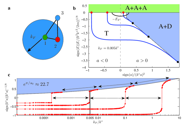
Figure 1: Efimov spectrum in the presence of a Fermi sea. a Schematic picture of the three interacting particles with a Fermi sea in the third component (blue filled circle). b Solid blue lines show the binding energies of the Efimov trimers (T), while the thin black lines mark the beginning of the A+A+A three-atom (upper) and A+D atom-dimer (right) continua. The intersection of the Efimov states with these continua are marked with red and black dots, respectively. The Fermi wave number is $k_{\rm{F}}=0.005k^{*}$. Here $k^{*}$ is the three-body parameter. Notice in particular how the least bound Efimov trimer has moved to the right of the resonance where the scattering length diverges and is a well-defined three-body bound state in spite of the presence of a bound two-body dimer. A thick black line marks the region where the Fermi energy is a relevant energy scale and influences the spectrum. This region grows with $k_{\rm{F}}$ and modifies the trimers to move towards the atom-dimer threshold roughly when they are inside the circle. Dashed lines mark the resonance (vertical) and the dimer threshold in vacuum (diagonal). c The spectrum flow of the Efimov trimers with zero three-body energy as function of $k_{\rm{F}}$. The solid black line indicates the position of the two-body atom-dimer threshold. The vertical axis has been scaled for visibility. The successive trimer thresholds scale with $e^{\pi/s_{0}}\sim 22.7$ for small $k_{\rm{F}}/k^{*}$, when they cross the resonance position as $k_{\rm{F}}$ increases, and again as they merge with the atom-dimer continuum.

As we will now discuss, the universal scaling laws, originally obtained by Efimov, hold also in the presence of a Fermi sea. Furthermore, we find a new scaling law related to the background Fermi energy, which may be interpreted as a many-body scaling for the three-body bound states. Our results demonstrate that the Efimov effect is robust in a many-body background. We consider first the generic problem of Efimov; three particles interacting with the same two-body interaction which is characterized by the scattering length, $a$, in the universal regime ($|a|\gg r_{0}$ with $r_{0}$ the characteristic potential range). Afterwards, we discuss the three-body bound states in the three-component ⁶Li system that has been recently realized [10, 11, 12]. For the latter system, we expect our findings to be accessible at or slightly above the densities of current experiments.

Our approach to the problem of three-body states in the presence of a background Fermi sea uses the momentum-space equations originally formulated by Skorniakov and ter-Martirosian (STM) [23, 24, 25]. In the absence of a Fermi sea, it has been shown [26, 25] that our approach captures the full physics of the Efimov effect, and in vacuum it is equivalent to the Faddeev decomposition in the hyperspherical formalism applied to the lowest hyperradial potential which also captures the Efimov effect [2]. We consider the case where one of the three particles forming the bound state has a Fermi sea with Fermi wave number, $k_{\rm{F}}$, in the limit of an inert sea with no particle-hole pairs. We will address the consequences of this approximation and also the case of multiple Fermi seas below. Since we are interested in the universal properties of the three-body spectrum we work exclusively with zero-range interaction that can be parametrized by $a$, but note that finite range corrections are easily taken into account in the STM approach. The scale of the spectrum is set by the three-body parameter $k^{*}$ [26]. Other recent studies considered similar issues in the Born-Oppenheimer limit [27, 28], where the fermion mass is much smaller than the two impurities, and using variational wave functions [29] inspired by the original work on the two-body Fermi polaron problem by Chevy [30]. The spectrum for $1/a=0$ as function of $k_{\rm{F}}$ was obtained using a semi-classical approximation in the Born-Oppenheimer limit [28]. Our approach using the STM equation is, however, general and works for any choice of masses and any value of the interaction strengths. An independent study of Pauli blocking effects was presented in Ref. [31]. That study did not address the scaling relations of Efimov states in the presence of a Fermi sea.

In the presence of a Fermi sea, the two-body dimer threshold moves from $1/a=0$ to the $a>0$ side of the two-body scattering resonance [32] as seen in figure 1b. Based on this observation, it is natural to speculate that the three-body bound state threshold with the continuum will also be moved as function of $k_{\rm{F}}$. We indeed confirm this expectation, but find that the states move in a fashion that respects the original scaling found by Efimov. Note that the the Efimov scaling is indeed violated for non-zero $k_{\rm{F}}$. This is clearly seen in figure 1b where the first and second Efimov trimers have 22.7 scaling, while the third one does not (see also figure 1c). In figure 1b we have chosen a value of $k_{\rm{F}}$ such that a bound three-body state merges with the three-body continuum at zero energy for $a>0$. This is perhaps puzzling since in the case of a single Fermi sea, a dimer could be formed between the two particles that do not have a background. However, we find numerically that the three-body state is well-defined in this region, i.e. the three-body energy has a vanishingly small imaginary part, and Pauli blocking thus seems to stabilize the system from decay into a dimer and an atom.

The famous Efimov scaling factor, $e^{\pi/s_{0}}\sim 22.7$, where $s_{0}=1.00624$ for equal mass particles, can be seen for $k_{\rm{F}}=0$ both on resonance ($1/a=0$) and at the thresholds on either side as a factor determining the ratio of energies and (dis)-appearance points [26, 33]. However, when we start to increase $k_{\rm{F}}$, we find a new type of scaling law related to the threshold behavior as function of $k_{\rm{F}}$. In figure 1c, we plot the flow of the critical points, $a_{n}^{-}$, where a three-body bound state appears from the three-atom continuum at zero energy as $k_{\rm{F}}$ is increased. These are marked with the red dots in figure 1b. On the far left of figure 1c in the limit $k_{\rm{F}}\to 0$, we see the usual scaling relation. As the thresholds, $a_{n}^{-}$, start to move they approach the two-body dimer threshold (black solid line in figure 1c) in a very systematic fashion.

The solutions shown in figure 1c are clearly self-similar. This is a hallmark of universal behavior. We find that a scaling law governs the relation between $a_{n}^{-}$ and $k_{\rm{F}}$. The $k_{\rm{F}}$ values for which an Efimov trimer threshold crosses resonance (nearly vertical ’jumps’ in figure 1c) are given by the universal relation

$$k_{\rm{F}}^{(n)}=\alpha e^{n\pi/s_{0}}k^{*},$$ (1)

where $\alpha$ is a non-universal constant that sets the overall scale. Recall that this relation connects a feature of the background, $k_{\rm{F}}$, and a feature of the universal, vacuum three-body system, $s_{0}$. Considering that Pauli blocking should influence low-momentum states, while the scaling laws are derived from the high-momentum behaviour [26], our results are highly non-trivial. The usual derivation of the Efimov scaling relation in vacuum will in fact be hindered by an obstructing term at low momentum, and the recovery of the scaling form is not obvious. The scaling with $k_{\rm{F}}$ is also found for the points at which the trimer merges with the atom-dimer continuum as seen in figure 1c. When considering either the ratios of the trimer energies on resonance (where Efimov originally found the infinite tower of universal states), or for the critical scattering length at which the trimers merge with the atom-dimer continuum at non-zero three-body energy (the black dots in figure 1b) we again find the same behavior when varying $k_{\rm{F}}$. The scaling on resonance was obtained previously in Ref. [28] but only in the limit of very large mass difference. While the results presented here have assumed equal mass particles, we find the same behavior for different masses when $s_{0}$ is changed accordingly. We address the advantages of using different mass ratios below.

Above we assume an inert Fermi sea. This is expected to be a good approximation on the $a<0$ side of the resonance. When interactions are present one must in general consider the effects of exciting particle-hole pairs in the Fermi sea. In principle, this can be done in a self-consistent manner through dressed particle-hole propagators which is numerically very difficult. The formalism can, however, be used to take corrections to the inert sea into account order by order (similar to the discussion in Ref. [34]). To estimate these effects, we have used a $k_{\rm{F}}$-dependent effective scattering length that includes the well-known Gorkov-Melik-Barkudarov particle-hole fluctuations (see Appendix A.1). We find that while the positions of thresholds will move, the scaling law discussed above remains the same. This suggests that our findings could be robust even when including particle-hole correlations, and indicates the generic nature of Efimov scaling even in the presence of a Fermi sea. However, there are some intrinsic differences between the two- and three-body problems which can for instance be seen in the rather smooth behavior of the two-body wave function through the BCS-BEC crossover in contrast to the oscillatory nature of the Efimov three-body wave function. Further studies of the influence of particle-hole correlations on the Efimov effect are therefore necessary to test its robustness in this type of many-body environment. Furthermore, we caution that our estimates of the particle-hole effects will become much worse and eventually break down on the BEC side of the resonance where strongly bound dimers are present in the system. Monte Carlo calculations [35] find a two-body dimer threshold that is larger than results from low-order diagrammatical calculations [36]. While it has been shown that when including the effects of single particle-hole pairs, the result is in very good agreement with Monte Carlo calculations even on the BEC side [30, 34, 37, 38, 39] (see Appendix A.1), this does not necessarily imply similar good agreement for the more complicated Efimov three-body systems and further studies are warranted. In any case, for the observation of Efimov physics and the results discussed here it is not necessary to approach the deep BEC regime.

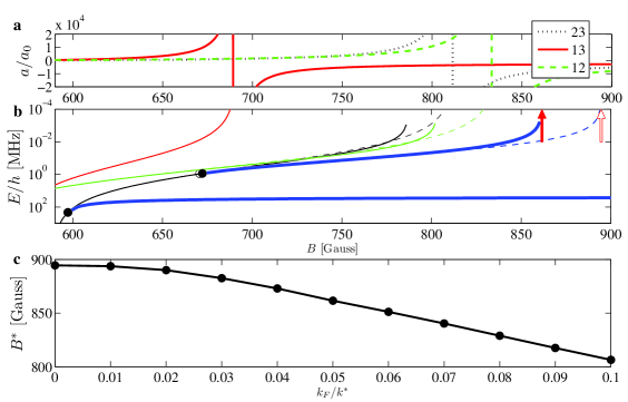
Figure 2: Trimer spectrum for a three-component ⁶Li system in the presence of a Fermi sea. a Scattering length and b energies as function of magnetic field when state $|2\rangle$ has a Fermi sea with $k_{\rm{F}}=0.05k^{*}$ (using labels from Ref. [11]). The dashed lines are the results with no Fermi sea. Black dots indicate the intersections of the trimers with the atom-dimer thresholds. The threshold of the second trimer state in the presence of a Fermi sea is marked by a red arrow, while a white arrow indicates the position with no Fermi background. c Magnetic field position, $B^{*}$, of the second Efimov trimer threshold (red arrow in b) as $k_{\rm{F}}$ is increased.

We now turn to the experimental signatures of a many-body background on Efimov physics. The signature we will discuss is the loss peak observed at the threshold for three-body bound state formation from the three-atom continuum on the $a<0$ side of a Feshbach resonance. Our assumption will be that this peak is moved as the Fermi sea modifies the binding energy of the three-body state and thus the threshold value. A more precise way would be to include a (small) imaginary part in the three-body parameter or in the real-space three-body potential to simulate the loss [26, 40]. This can typically produce both a peak position and shape. However, here we focus only on the peak and assume that it follows the threshold as in the vacuum case. The question of what happens to the shape of the peak in the presence of a Fermi sea will be left for future studies.

Presently, the experimentally most relevant system is the three-component ⁶Li gas where signatures of Efimov states have been observed by a number of groups in mixtures comprised of the three lowest atomic hyperfine states, conventionally labelled $|1\rangle$, $|2\rangle$ and $|3\rangle$ [10, 11, 12]. The variation of the scattering lengths $a_{ij}$ with an applied magnetic field exhibits three broad Feshbach resonances as shown in figure 2a. In figure 2b and c, we present results for a Fermi sea in hyperfine state $|2\rangle$. We predict a clear displacement of the magnetic field position at which the second Efimov trimer merges with the continuum, which becomes more pronounced as $k_{\rm{F}}$ increases. This state has been observed as a resonant three-body loss peak at densities $5\times 10^{9}$ atoms/cm³ at a temperature of 30 nK [41] and used to determine the three-body parameter $k^{*}=6.9(2)\times 10^{-3}\,a_{0}^{-1}$ ($a_{0}=5.29\cdot 10^{-11}$ m). We use this value of $k^{*}$ in figure 2, which can be converted to a density through $k_{\rm{F}}/k^{*}=3\cdot 10^{-6}(n/\textrm{cm}^{-3})^{1/3}$. Notice that the trimer state we consider is on the BCS side of the resonance and we expect particle-hole correlation effects to be small as discussed above. We estimate that the density used in Ref. [10] to be too low to see the effect of the Fermi sea (see figure 2c). Therefore the experiment provides a consistent estimation of $k^{*}$. While larger densities have been used [10, 12, 42], no results for the second trimer at large density have been reported.

In order for the presence of the many-body background to move the three-body loss resonance in the ⁶Li system by about 40 Gauss as shown in figure 2b, we estimate that densities of $5\cdot 10^{12}$ atoms/cm³ are required. In light of uncertainties in $k^{*}$ [41, 43], this estimate could increase by an order of magnitude. A potential problem of measuring the loss signal at finite $k_{\rm{F}}$ is that the trimer moves closer to the Feshbach resonance where the scattering length is very large. This reduces the so-called threshold regime where the loss feature is large [44]. The Fermi energy can reduce the observability in similar fashion. However, more recent results [45] indicate that universal physics is accessible even at finite collisional two-body energies. We expect this to hold true when adding the degenerate Fermi sea and that the movement of the loss peak from the second trimer state should be observable. Changing the energy of the first trimer on the other side of the resonance where a dimer exists and photo association is possible [11, 12] requires unrealistically high densities. We note that the differences in the ⁶Li scattering lengths can be reduced dramatically by applying additional optical fields [46], bringing the real system closer to the generic Efimov system considered above.

The ⁶Li system is in a sense not an optimal choice for observing the flow of the Efimov spectrum as equal mass systems has a large scaling factor, $e^{2\pi/s_{0}}$, so the trimer states are far apart in energy. On the other hand, if the mass ratio(s) are large, the spectrum is much denser [47]. Additionally, heteronuclear Feshbach resonances tend to have smaller background scattering lengths [48] which could be beneficial in order to not saturate the unitary limit and wash out the loss peak(s). Since we find that the movement of trimer energies with $k_{\rm{F}}$ and the scaling laws are generic in the universal limit, we expect that hetero-atomic mixtures are a much better options for observing these background effects when the fermionic component(s) has large density. We note that a very recent experiment at MIT [49] using mixtures of Bose and Fermi species fit very well with the requirements to make our predictions more readily observable. While we have focused on trimer energies, the STM equations are perfectly suited for calculating the loss rates [26, 50] and our work demonstrates how one can include effects of a degenerate background in these quantities.

Here we have only considered the case of a Fermi sea in a single component of the trimer system. As the three-body Efimov physics depends mostly on two-body subsystem thresholds, we expect to find qualitatively similar results with additional Fermi seas (see discussion in the supplementary material). We do expect that with two Fermi seas one could have Cooper pairs for any $a$, and in turn the dimer threshold would go to $a\to 0^{-}$. This extends the atom-dimer continuum and one can imagine that the trimer thresholds also move toward $a\to 0^{-}$. However, the binding energy of Cooper pairs is exponentially small in that limit and there could still be a critical value $a^{-}<0$ for forming trimers. An additional question is the effect of superfluidity at low temperatures. This will presumably also change the spectrum, but we doubt that the scaling relation with $k_{\rm{F}}$ is modified. We note that many-body effects on trimers should be present in bosonic samples as well [51] and will in some cases cause similar bound state energy spectral flow with background parameters (condensate density) [52] as seen in the present case with fermions. Recent experiments on ⁷Li with thermal and condensed samples find apparent discrepancies [7, 53], which could be attributed to effects of the finite range of the inter-atomic interactions [54]. It would be interesting to investigate whether the many-body background could also play a role. The approach pursued here should be applicable to bosonic systems as well, an obvious direction for future work. Lastly, the influence of a background environment on the recently measured four-body states [5, 7] is an interesting open question.

Appendix A Dressed Dimer Propagator.

The dressed dimer can be obtained from the Bethe-Selpeter equation in the ladder approximation [55]. Here we consider only a zero-range interaction, which amounts to a constant in momentum space. This leads to a dimer propagator (or two-body $T$-matrix) between atoms $i\neq j$ of the form

$$D_{ij}({\bf k},\omega)=T_{ij}({\bf k},\omega)=\frac{g_{ij}}{1-g_{ij}\Pi_{ij}({\bf k},\omega)},$$ (2)

where $\Pi_{ij}({\bf k},\omega)$ is the pair bubble and $g_{ij}$ is the coupling constant of the zero-range potential. Introducing a Fermi sea to be in component $j$ with Fermi wave number $k_{\rm{F}}$, the pair bubble at zero temperature becomes

$$\Pi_{ij}({\bf k},\omega) = \int\frac{d^{3}q}{(2\pi)^{3}}\,\frac{\Theta(q-k_{\rm{F}})}{\hbar\omega-\frac{\hbar^{2}q^{2}}{2m_{j}}-\frac{\hbar^{2}({\bf k}+{\bf q})^{2}}{2m_{i}}+\mu_{j}+i\epsilon},$$ (3)

where $m_{i}$ and $m_{j}$ are the particle masses, $\mu_{j}=\hbar^{2}k^{2}_{\rm{F}}/2m_{j}$ the chemical potential of component $j$ and $\epsilon$ is an infinitesimal positive number. At zero temperature, we see that the dimer propagator is modified by a restriction of Hilbert space due to Pauli blocking in one of the components as the Fermi sea is introduced. The usual linear divergence at large momentum with the momentum cut-off, $\Lambda$, persists when modifying the Hilbert space at low momentum through $k_{\rm{F}}$. This is renormalized through the two-body scattering length $a_{ij}$ which can be related to the vacuum ($k_{\rm{F}}=0$) $T$-matrix, $T^{0}_{ij}$, by

$$a_{ij}=\frac{m_{ij}}{2\pi\hbar^{2}}T^{0}_{ij}(0,0)=\frac{\frac{m_{ij}}{2\pi\hbar^{2}}}{g^{-1}_{ij}+\frac{m_{ij}\Lambda}{\pi^{2}\hbar^{2}}},$$ (4)

where $m_{ij}=m_{i}m_{j}/(m_{i}+m_{j})$ is the reduced mass of the dimer. The renormalized dimer propagator is

$$D_{ij}({\bf k},\omega)=\frac{2\pi\hbar^{2}}{m_{ij}}\frac{1}{a_{ij}^{-1}-\frac{\sqrt{2m_{ij}}}{\hbar}\sqrt{-\hbar\omega+\frac{\hbar^{2}k^{2}}{2M_{ij}}-\mu_{j}-i\epsilon}+R({\bf k},\omega)},$$ (5)

where the contribution of the Fermi sea in component $j$ is seen in the chemical potential, $\mu_{j}$, and the many-body correction term

$$R({\bf k},\omega)=\frac{m_{i}k}{2\pi m_{ij}}\biggl{\{}2\frac{m_{ij}}{m_{i}}x_{\rm{F}}-\frac{x_{\rm{F}}^{2}}{2}\ln\left[\frac{(x_{\rm{F}}-x_{+})(x_{\rm{F}}-x_{-})}{(x_{\rm{F}}+x_{+})(x_{\rm{F}}+x_{-})}\right]$$

$$-\frac{x_{+}^{2}}{2}\ln\left(\frac{x_{\rm{F}}+x_{+}}{-x_{\rm{F}}+x_{+}}\right)-\frac{x_{-}^{2}}{2}\ln\left(\frac{x_{\rm{F}}+x_{-}}{-x_{\rm{F}}+x_{-}}\right)\biggr{\}},$$ (6)

with $x_{\rm{F}}=\frac{k_{\rm{F}}}{k}$ and

$$x_{\pm}=\frac{m_{ij}}{m_{i}}\pm\sqrt{\left(\frac{m_{ij}}{m_{i}}\right)^{2}+\frac{2m_{ij}(\hbar\omega+\mu_{j})}{\hbar^{2}k^{2}}-\frac{m_{ij}}{m_{ik}}+i\epsilon}.$$ (7)

The bound state pole of equation (5) is used to determine the boundary of the atom-dimer continuum shown in figure 1b and 1c of the main text. We note that in the case of equal masses, the lowest energy state of the dimer is always at zero center-of-mass momentum. In fact, this is true whenever $m_{i}\geq m_{j}$ with $j$ having the Fermi sea. However, this is not a necessary assumption in our setup which works just as well for $m_{i}<m_{j}$ where non-zero center-of-mass dimers may be lower in energy [32, 34, 56]. The critical scattering length, $a_{ij}^{c}$ at which the dimer pole appears at zero energy, $E=0$, in the presence of a Fermi sea has the analytical expression

$$\frac{1}{a_{ij}^{c}}=\frac{2k_{\rm{F}}}{\pi}\left(1-\frac{1}{2}\sqrt{\frac{m_{ij}}{m_{j}}}\ln\left|\frac{1+\sqrt{m_{j}/m_{ij}}}{1-\sqrt{m_{j}/m_{ij}}}\right|\right).$$ (8)

In the equal mass case we have $\frac{1}{a_{ij}^{c}}=0.24k_{F}$ which marks the edge of the atom-dimer continuum in figure 1c of the main text.

A.1 Higher-order Corrections

Here we discuss an estimate of the effect of particle-hole pairs in the two-body dimer, i.e. of a system of two-component fermions. As the two-body propagator enters the calculation of the three-component system it should yield an insight into how this affects the three-body states.

The dimer propagator in (5) is obtained from the ladder approximation to lowest order. At next order, we need to include the effect of particle-hole excitations in the Fermi sea in analogy to what has been discussed in fermionic superfluids by Gor’kov and Melik-Barkhudarov [57]. As shown in Ref. [36], this can be achieved by using an effective scattering length, $\tilde{a}_{ij}$, given by

$$\tilde{a}_{ij}^{-1}=a_{ij}^{-1}-Fk_{\rm{F}},$$ (9)

where $F$ contains the lowest order vertex correction and depends on the mass ratio $m_{i}/m_{j}$. For $m_{i}=m_{j}$, $F\sim 0.2$. To check the robustness of our finding we have calculated trimer energies with $a_{ij}$ replaced by $\tilde{a}_{ij}$, and we have also varied the value of $F$. While this modifies the absolute values of the binding energies, it does not alter the scaling relation in $k_{\rm{F}}$. We therefore believe that the scaling is unaltered by vertex corrections.

Diagrammatic Monte Carlo studies of the strongly imbalanced two-component Fermi system (the so-called polaron problem) [35] does, however, show that the critical scattering length is $(k_{\rm{F}}a_{ij}^{c})^{-1}=0.88$, which is higher than both the lowest order ladder approximation ($(k_{\rm{F}}a_{ij}^{c})^{-1}=0.24$) and the result including particle-hole correlations ($(k_{\rm{F}}a_{ij}^{c})^{-1}=0.34$). As noted in Ref. [36], this implies that the vertex corrections are qualitatively correct but underestimate the effect of higher-order corrections. In the polaron problem it has been shown that inclusion of one particle-hole pair correlations on top of the inert Fermi sea gives results that are similar to the Monte Carlo findings [37, 34, 38, 39]. In a $T$-matrix approach such as the one used here, these corrections can be taken systematically into account through self-energy terms.

We note that the dimer propagator in (5) is not accurate in the deep BEC limit ($a\to 0^{+}$) where it can be shown to yield the Born approximation for the atom-dimer scattering length, $a_{3}/a_{ij}=8/3$, which overestimates the exact result of $a_{3}/a_{ij}=1.18$ originally obtained in Ref. [23] and subsequently reproduced and discussed by several authors, see for instance Ref. [34]. We believe that all these corrections should be only quantitative a more detailed analysis that takes the self-energy term in the single-particle propagators and higher-order terms in the dimer propagator is necessary to confirm this. Quantitatively, we expect the present treatment to work well for $a_{ij}<0$ and around the resonance, $1/a_{ij}\to 0$. However, observing the Efimov scaling in $k_{\rm{F}}$ does not require calculations in the deep BEC limit as demonstrated in figure 1 of the main text and our findings should be recovered in more involved treatments.

A.2 Additional Fermi seas

The considerations above pertain to the case where one of the particles that make up the three-body bound state has a background Fermi sea. A natural extension is to consider two or three Fermi seas. The STM equations that we use can perfectly well accommodate such a system when properly modifying the dimer propagator. For the case of two Fermi seas, the pair bubble of (3) must be replaced by

$$\Pi_{ij}({\bf k},\omega)=\int\frac{d^{3}q}{(2\pi)^{3}}\,\frac{1-\Theta(k_{\rm{F}}-q)-\Theta(k_{\rm{F}}-|{\bf q}+{\bf k}|)}{\hbar\omega-\frac{\hbar^{2}q^{2}}{2m_{j}}-\frac{\hbar^{2}({\bf k}+{\bf q})^{2}}{2m_{i}}+\mu_{i}+\mu_{j}+i\epsilon},$$ (10)

where we assume two inert seas and thus propagation of a pair of particles above the Fermi seas only. We are also assuming that the two seas have the same size, $k_{\rm{F}}$, but this is not essential and can be easily generalized to imbalanced systems. The pair propagator above must be computed numerically in general. This form of the propagator appears for instance in the original work of Galitskii on the Fermi gas with strong short-range interactions [55, 58].

The goal of the current section is, however, to argue that the Efimov scaling in $k_{\rm{F}}$ discussed in the main text is maintained in the case of two Fermi seas. This can be done by considering the structure of the pair bubble in the limit where the center-of-mass momentum, ${\bf k}$, vanishes. Here we obtain

$$D_{ij}({\bf 0},\omega)=\frac{2\pi\hbar^{2}}{m_{ij}}\frac{1}{a_{ij}^{-1}-\frac{\sqrt{2m_{ij}}}{\hbar}\sqrt{-\hbar\omega-\mu_{i}-\mu_{j}-i\epsilon}+2R({\bf 0},\omega)},$$ (11)

in the limit ${\bf k}\to 0$. In the expression for $R({\bf 0},\omega)$ one must also make the substitution $\mu_{j}\to\mu_{j}+\mu_{i}$. This holds in the equal mass case and for an unpolarized system with Fermi seas in both components. In particular, this has the same structure as the case of a single Fermi sea discussed above. We have checked numerically that multiplication of $R({\bf 0},\omega)$ by two does not alter the scaling relations discussed in the main text. In the limit of small $k_{\rm{F}}$, $R({\bf 0},\omega)$ is proportional to $k_{\rm{F}}$. This shows that the changes required from addition of a second Fermi sea are similar to those coming from Gor’kov-Melik-Barkhudarov corrections above. While threshold will change, the overall scaling properties remain the same. We note that the shift of the critical value for a two-body bound state in the presence of a Fermi sea to the $a_{ij}>0$ side of the Feshbach resonance continues to hold true with Fermi seas in both components [59].

The argument given was for the case of vanishing center-of-mass momentum of the pairs in the dimer propagator. It is known from the Cooper pair problem that the strongest bound pairs have zero center-of-mass momentum [55]. Thus for the equal mass three-body states we expect this dimer pole to dominate, validating the arguments given above. Extension to three Fermi seas is straightforward and since the propagators are the same the same arguments can be used to infer that the scaling should persist there as well. If one considers the interesting case of unequal mass systems this may no longer be the case and the strongest bound two-body state may acquire non-zero center-of-mass momentum. All this can be studied within our formalism and we are actively pursuing this direction at the moment.

Appendix B Momentum-space Three-body Equations.

The momentum-space three-body equations are also known as the Skorniakov-ter-Martirosian equations (STM) [23] and where originally developed for problems in nuclear physics. By a ladder summation over all pairwise interactions the integral equations for the three-body $T$-matrix can be casts as the scattering of a dimer with an unbound atom. In a three component mixture there are thus three entrance channels and three exit channels for the free atom giving a $3\times 3$ $T$-matrix $T_{ij}$ [60]. The equations for the three-body scattering amplitudes, $T_{ij}(p,q)$, with a single Fermi sea in component $3$ after angular-averaging to get the zero angular momentum part are ($i=1,2,3$)

$$T_{i1}(p,q)=\sum_{k=1}^{3}(1-\delta_{i1})(1-\delta_{ik})(1-\delta_{1k})K_{i1}^{k}(p,q)$$

$$+\frac{1}{4\pi^{2}}\int_{-1}^{1}d(\cos\theta)\int_{0}^{\Lambda}dQ\,Q^{2}\times$$

$$\frac{2m_{23}\Theta(Q^{2}+q^{2}+2Qq\cos\theta-k_{\rm{F}}^{2})D_{13}\left({\bf Q},E-\frac{\hbar^{2}Q^{2}}{2m_{2}}\right)T_{i2}(p,Q)}{2m_{23}E-\hbar^{2}Q^{2}-\frac{m_{23}}{m_{13}}\hbar^{2}q^{2}-2\frac{m_{23}}{m_{3}}\hbar^{2}Qq\cos\theta+i0^{+}}$$

$$-\frac{1}{2\pi^{2}}\int_{k_{\rm{F}}}^{\Lambda}dQ\,Q^{2}K_{31}^{2}(Q,q)D^{0}_{12}\left({\bf Q},E-\frac{\hbar^{2}Q^{2}}{2m_{3}}\right)T_{i3}(p,Q),$$ (12)

$$T_{i2}(p,q)=\sum_{k=1}^{3}(1-\delta_{i2})(1-\delta_{ik})(1-\delta_{2k})K_{i2}^{k}(p,q)$$

$$+\frac{1}{4\pi^{2}}\int_{-1}^{1}d(\cos\theta)\int_{0}^{\Lambda}dQ\,Q^{2}\times$$

$$\frac{2m_{13}\Theta(Q^{2}+q^{2}+2Qq\cos\theta-k_{\rm{F}}^{2})D_{23}\left({\bf Q},E-\frac{\hbar^{2}Q^{2}}{2m_{1}}\right)T_{i1}(p,Q)}{2m_{13}E-\hbar^{2}Q^{2}-\frac{m_{13}}{m_{23}}\hbar^{2}q^{2}-2\frac{m_{13}}{m_{3}}\hbar^{2}Qq\cos\theta+i0^{+}}$$

$$-\frac{1}{2\pi^{2}}\int_{k_{\rm{F}}}^{\Lambda}dQ\,Q^{2}K_{32}^{1}(Q,q)D^{0}_{12}\left({\bf Q},E-\frac{\hbar^{2}Q^{2}}{2m_{3}}\right)T_{i3}(p,Q),$$ (13)

$$T_{i3}(p,q)=\sum_{k=1}^{3}(1-\delta_{i3})(1-\delta_{ik})(1-\delta_{3k})K_{i3}^{k}(p,q)$$

$$-\frac{1}{2\pi^{2}}\int_{0}^{\Lambda}dQ\,Q^{2}K_{13}^{2}(Q,q)D_{23}\left({\bf Q},E-\frac{\hbar^{2}Q^{2}}{2m_{1}}\right)T_{i1}(p,Q)$$

$$-\frac{1}{2\pi^{2}}\int_{0}^{\Lambda}dQ\,Q^{2}K_{23}^{1}(Q,q)D_{13}\left({\bf Q},E-\frac{\hbar^{2}Q^{2}}{2m_{2}}\right)T_{i2}(p,Q),$$ (14)

where the Heaviside step function $\Theta(x)$ is 1 for $x>0$ and vanishes for $x<0$ and $E$ is the three-body energy. The superscript ’0’ on the dimer propagator $D^{0}_{12}$ is a reminder that it does not contain a Fermi sea and is the vacuum expression which can be recovered from (5) by setting $\mu_{j}=0$ and $R({\bf k},\omega)=0$. The kernel, $K_{ij}^{k}(p,q)$, is defined by

$$K_{ij}^{k}(p,q)=\frac{m_{k}}{2\hbar^{2}pq}\ln\left[\frac{p^{2}+\frac{m_{ik}}{m_{jk}}q^{2}+2\frac{m_{ik}}{m_{k}}pq-\frac{2m_{ik}E}{\hbar^{2}}}{p^{2}+\frac{m_{ik}}{m_{jk}}q^{2}-2\frac{m_{ik}}{m_{k}}pq-\frac{2m_{ik}E}{\hbar^{2}}}\right].$$ (15)

Since we are only interested in the spectrum of bound states in the present work, we neglect the homogeneous terms and use a standard pole expansion technique [61] by which we can write

$$T_{ij}(p,q)=\frac{B_{i}(p)B_{j}(q)}{E-E_{T}},$$ (16)

where $E_{T}$ is the trimer energy that we want to determine, and $B_{i}(p)$ are the residues at the poles, which represent the three-component bound state wave function. This yields the bound state equations

$$B_{1}(p)=\frac{1}{4\pi^{2}}\int_{-1}^{1}d(\cos\theta)\int_{0}^{\Lambda}dq\,q^{2}\times$$

$$\frac{2m_{23}\Theta(q^{2}+p^{2}+2qp\cos\theta-k_{\rm{F}}^{2})D_{13}\left({\bf q},E-\frac{\hbar^{2}q^{2}}{2m_{2}}\right)B_{2}(q)}{2m_{23}E-\hbar^{2}q^{2}-\frac{m_{23}}{m_{13}}\hbar^{2}p^{2}-2\frac{m_{23}}{m_{3}}\hbar^{2}qp\cos\theta+i0^{+}}$$

$$-\frac{1}{2\pi^{2}}\int_{k_{\rm{F}}}^{\Lambda}dq\,q^{2}K_{31}^{2}(q,p)D^{0}_{12}\left({\bf q},E-\frac{\hbar^{2}q^{2}}{2m_{3}}\right)B_{3}(q),$$ (17)

$$B_{2}(p)=\frac{1}{4\pi^{2}}\int_{-1}^{1}d(\cos\theta)\int_{0}^{\Lambda}dq\,q^{2}\times$$

$$\frac{2m_{13}\Theta(q^{2}+p^{2}+2qp\cos\theta-k_{\rm{F}}^{2})D_{23}\left({\bf q},E-\frac{\hbar^{2}q^{2}}{2m_{1}}\right)B_{1}(q)}{2m_{13}E-\hbar^{2}q^{2}-\frac{m_{13}}{m_{23}}\hbar^{2}p^{2}-2\frac{m_{13}}{m_{3}}\hbar^{2}qp\cos\theta+i0^{+}}$$

$$-\frac{1}{2\pi^{2}}\int_{k_{\rm{F}}}^{\Lambda}dq\,q^{2}K_{32}^{1}(q,p)D^{0}_{12}\left({\bf q},E-\frac{\hbar^{2}q^{2}}{2m_{3}}\right)B_{3}(q),$$ (18)

$$B_{3}(p)=-\frac{1}{2\pi^{2}}\int_{0}^{\Lambda}dq\,q^{2}\times$$

$$K_{13}^{2}(q,p)D_{23}\left({\bf q},E-\frac{\hbar^{2}q^{2}}{2m_{1}}\right)B_{1}(q)$$

$$-\frac{1}{2\pi^{2}}\int_{0}^{\Lambda}dq\,q^{2}K_{23}^{1}(q,p)D_{13}\left({\bf q},E-\frac{\hbar^{2}q^{2}}{2m_{2}}\right)B_{2}(q).$$ (19)

The original STM equations are divergent at large momenta and a cut-off, $\Lambda$, is necessary on the integrals. This is caused by the well-known Thomas collapse [62]. The equations therefore need to be regularized which can be done in a number of different ways [26]. Here we use the elegant subtraction technique of Pricoupenko [25], which draws inspiration from the older work of Danilov [24] on how to impose conditions on the asymptotic (high-momentum) behaviour. After regularization, the equations become ($i\neq j\neq k$)

$$B_{i}(p)=-\frac{1}{2\pi^{2}}\int_{0}^{\Lambda}dq\,q^{2}\times$$

$$\left[\Delta{\mathcal{K}}_{ki}^{j}(q,p)D_{ij}\left({\bf q},E-\frac{\hbar^{2}q^{2}}{2m_{k}}\right)B_{k}(q)\right.$$

$$\left.+\Delta{\mathcal{K}}_{ji}^{k}(q,p)D_{ik}\left({\bf q},E-\frac{\hbar^{2}q^{2}}{2m_{j}}\right)B_{j}(q)\right],$$ (20)

where $\Delta{\mathcal{K}}_{ij}^{k}(q,p)={\mathcal{K}}_{ij}^{k}(q,p)-{\mathcal{K}}_{ij}^{k}(q,k_{\rm{reg}})$, and we have defined

$${\mathcal{K}}_{3j}^{k}(q,p)=K_{3j}^{k}(q,p)\Theta(q-k_{\rm{F}}),$$ (21)

$${\mathcal{K}}_{i3}^{k}(q,p)=K_{i3}^{k}(q,p),$$ (22)

$${\mathcal{K}}_{ij}^{3}(q,p)=-\frac{1}{2}\int_{-1}^{1}d(\cos\theta)\times$$

$$\frac{2m_{i3}\Theta(q^{2}+p^{2}+2qp\cos\theta-k_{\rm{F}}^{2})}{2m_{i3}E-\hbar^{2}q^{2}-\frac{m_{i3}}{m_{j3}}\hbar^{2}p^{2}-2\frac{m_{i3}}{m_{3}}\hbar^{2}qp\cos\theta+i0^{+}}.$$ (23)

The parameter in the regularizing part of the kernel can be expressed as [25]

$$\frac{k_{\rm{reg}}}{k^{*}}=\frac{1}{\sqrt{3}}e^{\pi(n+1)/s_{0}},$$ (24)

where $k^{*}$ is the three-body parameter which the basic unit in the three-body problem and which cannot be determined within the universal theory containing only scattering length parameters [26]. Here $s_{0}$ is the scale factor and $n$ is a normalization factor which fixes the minimum energy of trimer states [25]. In all our numerical calculations we use $n=0$. The regularization scheme is derived in the large momentum limit where the equations become scale invariant. The inclusion of a Fermi sea does not alter the asymptotic behavior and the same regularization can therefore be used in this case also.

References

References

- [1] Efimov V 1970 Yad. Fiz. 12 1080; 1971 Sov. J. Nucl. Phys. 12 589; 1973 Nucl. Phys. A 210 157
- [2] Jensen A S, Riisager K, Fedorov D V and Garrido E 2004 Rev. Mod. Phys. 76 215
- [3] Bloch I, Dalibard J and Zwerger W 2008 Rev. Mod. Phys. 80 885
- [4] Kraemer T et al. 2006 Nature 440 315
- [5] Ferlaino F et al. 2009 Phys. Rev. Lett. 102 140401
- [6] Barontini G et al. 2009 Phys. Rev. Lett. 103 043201
- [7] Pollack S E, Dries D and Hulet R G 2009 Science 326 1683
- [8] Zaccanti M et al. 2009 Nature Phys. 5 586
- [9] Gross N et al. 2009 Phys. Rev. Lett. 103 163202
- [10] Huckans J H et al. 2009 Phys. Rev. Lett. 102 165302
- [11] Lompe T et al. 2010 Science 330 940
- [12] Nakajima S et al. 2011 Phys. Rev. Lett. 106 143201
- [13] Machtey O, Shotan Z, Gross N and Khaykovich L 2012 Phys. Rev. Lett. 108 210406
- [14] Rem B S et al. 2013 Phys. Rev. Lett. 110 163202
- [15] Roy S et al. 2013 Phys. Rev. Lett. 111 053202
- [16] Cooper L N 1956 Phys. Rev. 104 1189
- [17] Bardeen J, Cooper L N and Schrieffer J R 1957 Phys. Rev. 106 162 ; ibid 108 1175
- [18] Partridge G B, Li W, Kamar R I, Liao Y and Hulet R G 2006 Science 311 503
- [19] Shin Y et al. 2006 Phys. Rev. Lett. 97 030401
- [20] Zwierlein M W, Schirotzek A, Schunck C H and Ketterle W 2006 Science 311 492
- [21] Schirotzek A, Wu C-H, Sommer A and Zwierlein M W 2009 Phys. Rev. Lett. 102 230402
- [22] Nascimbene S et al. 2010 Nature 463 1057
- [23] Skorniakov G V and Ter-Martirosian K A 1956 Zh. Eksp. Teor. Fiz. 31 775
- [24] Danilov G 1961 Zh. Eksp. Teor. Fiz. 40 498
- [25] Pricoupenko L 2010 Phys. Rev. A 82 043633
- [26] Braaten E and Hammer H W 2006 Phys. Rep. 428 259
- [27] Nishida Y 2009 Phys. Rev. A 79 013629
- [28] MacNeill D J and Zhou F 2011 Phys. Rev. Lett. 106 145301
- [29] Mathy C J M, Parish M M and Huse D A 2011 Phys. Rev. Lett. 106 166404
- [30] Chevy F 2006 Phys. Rev. A 74 063628
- [31] Niemann P and Hammer H-W 2012 Phys. Rev. A 86 013628
- [32] Watanabe T, Suzuki T and Schuck P 2008 Phys. Rev. A. 78 033601
- [33] Nielsen E, Fedorov D V, Jensen A S and Garrido E 2001 Phys. Rep. 347 373
- [34] Combescot R, Giraud S and Leyronas X 2009 Europhys. Lett. 88 60007
- [35] Prokof’ev N and Svistunov B 2008 Phys. Rev. B 77 020408(R)
- [36] Song J-L and Zhou F 2011 Phys. Rev. A 84 013601
- [37] Combescot R and Giraud S 2008 Phys. Rev. Lett. 101 050404
- [38] Mora C and Chevy F 2009 Phys. Rev. A 80 033607
- [39] Punk M, Dumitrescu P T and Zwerger W 2009 Phys. Rev. A 80 053605
- [40] Sørensen P K, Fedorov D V, Jensen A S and Zinner N T 2013 Phys. Rev. A 88 042518
- [41] Williams J R et al. 2009 Phys. Rev. Lett. 103 130404
- [42] Ottenstein T B, Lompe T, Kohnen M, Wenz A N and Jochim S 2008 Phys. Rev. Lett. 101 203202
- [43] Nakajima S et al. 2010 Phys. Rev. Lett. 105 023201
- [44] D’Incao J P, Suno H and Esry B D 2004 Phys. Rev. Lett. 93 123201
- [45] Wang Y and Esry B D 2011 New J. Phys. 13 035025
- [46] O’Hara K M 2011 New J. Phys. 13 065011
- [47] Jensen A S and Fedorov D V 2003 Europhys. Lett. 62 336
- [48] Chin C, Grimm R, Julienne P S and Tiesinga E 2010 Rev. Mod. Phys. 82 1225
- [49] Wu C-H et al. 2011 Phys. Rev. A 84 011601(R)
- [50] Braaten E, Hammer H-W, Kang D and Platter L 2009 Phys. Rev. Lett. 103 073202
- [51] Zinner N T 2013 Europhysics Letters 101 60009
- [52] Zinner N T 2013 Preprint arXiv:1312.7821
- [53] Gross N, Shotan Z, Kokkelmans S and Khaykovich L 2010 Phys. Rev. Lett. 105 103203
- [54] Dyke P, Pollack, S E and Hulet R G 2013 Phys. Rev. A 88 023625
- [55] Fetter A L and Walecka J D 1971 Quantum Theory of Many-Particle Systems (McGraw-Hill, New York 1971)
- [56] Song J-L, Mashayekhi M S and Zhou F 2010 Phys. Rev. Lett. 105 195301
- [57] Gor’kov L P and Melik-Barkhudarov T M 1961 Sov. Phys. JETP 13 1018
- [58] Galitskii V M 1958 Sov. Phys. JETP 7 104
- [59] Combescot R 2003 New Jour. Phys. 5 86
- [60] Braaten E, Hammer H-W, Kang D and Platter L 2010 Phys. Rev. A 81 013605
- [61] Taylor J R Scattering Theory (Rev. ed. Robert E. Krieger Pub. Co., Malabar, Fla. 1983)
- [62] Thomas L H 1935 Phys. Rev. 47 903