Effect of dynamic and static friction on an asymmetric granular piston

Abstract

We investigate the influence of dry friction on an asymmetric, granular piston of mass $M$ composed of two materials undergoing inelastic collisions with bath particles of mass $m$. Numerical simulations of the Boltzmann-Lorentz equation reveal the existence of two scaling regimes depending on the strength of friction. In the large friction limit, we introduce an exact model giving the asymptotic behavior of the Boltzmann-Lorentz equation. For small friction and for large mass ratio $M/m$, we derive a Fokker-Planck equation for which the exact solution is also obtained. Static friction attenuates the motor effect and results in a discontinuous velocity distribution.

I Introduction

An adiabatic piston separating two compartments of gases is a widely studied model in statistical physics. The initial interest arose from the observation that the equilibrium state cannot be predicted by application of the First and Second laws of thermodynamics callen60 ; Piasecki1999 ; Gruber1999 ; Gruber2002 ; Gruber2003 . It was shown that dynamics contains different time scales before the system reaches equilibrium (for finite-size compartments) or a steady state where the piston acquires a non-zero drift velocity (for infinite compartments) Gruber2006 .

The granular version of the system, where the gas particles undergo dissipative collisions, also displays interesting behavior. Brito et. al Brito2005 showed that the piston eventually collapses to one side and Brey and Khalil PhysRevE.82.051301 showed that the steady state is characterized by equal cooling rates in the two compartments.

The model was investigated in the context of a granular motor by Costantini et al. costantini:061124 . They considered a piston composed of two different materials and showed that fluctuations on the right and left sides result in noise rectification that can be converted into mechanical work. When the bath density is low, the appropriate kinetic description of the system is the Boltzmann-Lorentz equation. However, an exact solution cannot be obtained even for this simple model. Costantini et al. Costantini2008 proposed an ansatz of the velocity distribution, where parameters are obtained by calculating successive moments of the kinetic equation. Comparisons with numerical simulations showed that the approach is reasonable, but it fails in the limit of large piston mass (the Brownian limit). Talbot et al. PhysRevE.82.011135 introduced a mechanical treatment that gives an exact expression for the drift velocity in the Brownian limit.

Recently, Eshuis et al. PhysRevLett.104.248001 presented the first experimental realization of a macroscopic, rotational ratchet in a granular gas. The device, which consists of four vanes, is reminiscent of that imagined by Smoluchowski smolu12 ; feymann63 . When a soft coating was applied to one side of each vane, a motor effect was observed above a critical granular temperature. While this was the first experimental realization of a granular motor, similar Brownian ratchets exist in many diverse applications, e.g., photovoltaic devices and biological motors; See Reimann2002 ; RevModPhys.69.1269 ; vandenBroekM.2009 . All of these motors share the common features of non-equilibrium conditions and spatial symmetry breaking. Several recent theoretical studies of idealized models of granular motors, which use a Boltzmann-Lorentz description Cleuren2007 ; Cleuren2008 ; Costantini2008 ; Costantini2009 ; PhysRevE.82.011135 , confirm that the motor effect is particularly pronounced when the device is constructed from two different materials, as was the case in the recent experiment PhysRevLett.104.248001 . The existing theories, however, predict a motor effect for any temperature of the granular gas while in the experiment the phenomenon is only observed if the bath temperature is sufficiently large.

Friction likely plays an important role in the experiment PhysRevLett.104.248001 as it does in other systems with stochastic dynamics. The first theoretical studies date from 2005 when de Gennes Gennes2005 and Hayakawa Hayakawa2005 addressed the effect of dry (Coulombic) friction on Brownian motion. Subsequently, Kawarada and Hayakawa JPSJ.73.2037 showed that the signature of Coulombic friction is an exponentially decaying velocity distribution function. Menzel and Goldenfeld PhysRevE.84.011122 studied a Fokker-Planck equation and noted a formal connection to the Schrödinger equation for the quantum mechanical oscillator with a delta potential. MaugerMauger2006 showed that the Coulomb friction is responsible for an exponential decay of the velocity distribution when dynamics is described by a Fokker-Planck equation. Touchette and coworkers Touchette2010 ; Baule2010 ; Baule2011 obtained a solution of a model with dry friction and viscous damping. Experimental studies have examined droplets on non-wettable surfaces subjected to an asymmetric lateral vibration A.Buguin2006 , as well as the biased motion of a water drop on a tilted surface subject to vibration Chaudhury2008 ; Goohpattader2009 ; Mettu2010 .

Recently, we used numerical simulation and kinetic theory to examine the effect of dynamic friction on a chiral rotor within the framework of the Boltzmann-Lorentz equation PhysRevLett.107.138001 . The numerical simulations revealed the existence of two scaling regimes at low and high bath temperatures. For large piston masses and small friction the model can be mapped onto a Fokker-Planck equation that can be solved analytically. We also obtained analytic solutions for the mean velocity and the velocity distribution function in the limit of large friction. The purpose of the present article is to present a complete analysis of the effect of dynamic and, for the first time, static friction on the asymmetric granular piston.

In Sec. II, we introduce the model of a granular piston with friction. We perform Monte Carlo simulations in Sec.III. A time scale analysis presented in Sec. IV suggests that the model can be solved in two limiting cases. In Sec.V, we first consider the high friction limit by introducing the independent kick model and compare the exact solution of the model with numerical simulations of the BL equation. In the Brownian limit and in the small friction limit, we show that the Fokker-Planck equation, for which analytical solutions can be obtained, provides an accurate description of the BL equation. In Sec.VII, we generalize our study by including the effect of static friction and we briefly conclude in Sec.VIII.

II The model

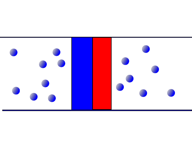
Figure 1: The asymmetric granular piston in a bath of thermalized particles.

An infinite cylinder filled with a monodisperse gas composed of particles of mass $m$ is separated into two compartments by a granular piston of mass $M$ and of vertical length $L$ that is composed of two materials characterized by the coefficients of restitution $\alpha_{+}$ and $\alpha_{-}$. The piston is constrained to move along the symmetric axis of the container and undergoes collisions with the gas particles. In addition, a frictional force of constant strength $F$, which acts to oppose the motion of the piston, is present. In the absence of the bath particles the equation of motion of the piston is

$$M\frac{dV}{dt}=-\sigma(V)F$$ (1)

where

$$\sigma(V)=\left\{\begin{array}[]{rl}+1&\mbox{ if $V>0$}\\ 0&\mbox{ if $V=0$}\\ -1&\mbox{ if $V<0$}\end{array}\right.$$ (2)

Due to the translational invariance along perpendicular axis of the container and assuming that the radius of the cylinder is sufficiently, boundary effects can be neglected. Consequently, the collision rules only involve the velocity component along the the cylinder axis. If $v$ and $V$ are the pre-collisional values, the post-collisional velocities of the piston and gas particles are

$$V^{\prime}_{\alpha_{\pm}}=V+\frac{1+\alpha_{\pm}}{1+\mu}(v-V)$$ (3)

$$v^{\prime}_{\alpha_{\pm}}=v-\frac{\mu(1+\alpha_{\pm})}{1+\mu}(v-V)$$ (4)

where $\mu=\frac{M}{m}$ is the mass ratio and $\alpha_{+}$ ($\alpha_{-}$) is selected if the collision occurs on the left (right) hand side of the piston, i.e. if $v-V>0$ ($v-V<0$).

Pre-collisional (or restituting) velocities $V^{\prime\prime}_{\alpha_{\pm}},v^{\prime\prime}_{\alpha_{\pm}}$ can be obtained from Eqs.(3-4) by replacing $\alpha_{\pm}$ with $\alpha_{\pm}^{-1}$.

The kinetic properties of the piston are described by means of the Boltzmann-Lorentz equation. Let us denote $f(V;t)$ the probability density of finding the piston moving with velocity $V$ and $\phi(v)$ represents the velocity distribution of the bath particles at time $t$, one has

$$\frac{\partial}{\partial t}f(V;t)-F\frac{\sigma(V)}{M}f(V;t)=J[\phi,f]$$ (5)

where $J[\phi,f]$ is the collision operator expressed as

$$J[f,\phi]=\rho L\int_{-\infty}^{\infty}dv\,|v-V|[\theta(v-V)\frac{f(V^{\prime\prime}_{\alpha_{+}};t)}{\alpha_{+}^{2}}$$

$$\left.\phi(v^{\prime\prime})+\theta(V-v)\frac{f(V^{\prime\prime}_{\alpha_{-}};t)}{\alpha_{-}^{2}}\phi(v^{\prime\prime})\right]-\rho L\nu(V)f(V;t)$$ (6)

where $\theta(u)$ is the Heaviside function and

$$\rho L\nu(V)=\rho L\int_{-\infty}^{\infty}dv|v-V|\phi(v)$$ (7)

is the collision rate of bath particles with (both sides of) the piston moving with a velocity $V$. Note that the Boltzmann-Lorentz equation neglects recollisions. This assumption is valid if the bath density is low and when the mass of the piston is larger than the mass of bath particles. In addition, the bath distribution, $\phi(v)$, is assumed stationary and symmetric such that $\langle v\rangle=0$.

By using appropriate changes of variablespiasecki:051307 , the kinetic equation can be rewritten as

$$\frac{1}{\rho L}\frac{\partial}{\partial t}f(V;t)-\frac{F\sigma(V)}{M\rho L}\frac{\partial}{\partial V}f(V;t)=\int_{0}^{\infty}dy\;y$$

$$\left[f\left(V-\frac{1+\alpha_{+}}{1+\mu}y;t\right)\phi\left(V+\frac{\mu-\alpha_{+}}{1+\mu}y\right)\right.$$

$$+\left.\;f\left(V+\frac{1+\alpha_{-}}{1+\mu}y;t\right)\phi\left(V-\frac{\mu-\alpha_{-}}{1+\mu}y\right)\right]$$

$$-f(V;t)\int_{0}^{\infty}dy\;y(\phi(V+y)+\phi(V-y))$$ (8)

It is convenient to introduce the reduced variables $F^{*}=F/(\rho LT)$ and $V^{*}=\sqrt{m/T}V$. With this choice the average drift velocity only depends on $F^{*}$, $M/m$ and $\alpha_{\pm}$. In an experiment, the frictional force depends on the physical properties of the motor and is not easily changed. On the other hand, the granular temperature of the bath particles can be varied simply by increasing or decreasing the vibration amplitude or frequency of the mechanical shaker driving the granular gas particles.

Where possible we give analytic results for a general bath particle velocity distribution, $\phi(v)$. For illustrative purposes, as well as to test the theory by comparison with numerical simulation of the BL equation, we will use a Gaussian distribution:

$$\phi(v)=\sqrt{\frac{m}{2\pi T}}\exp\left(-\frac{mv^{2}}{2T}\right)$$ (9)

III Numerical simulation

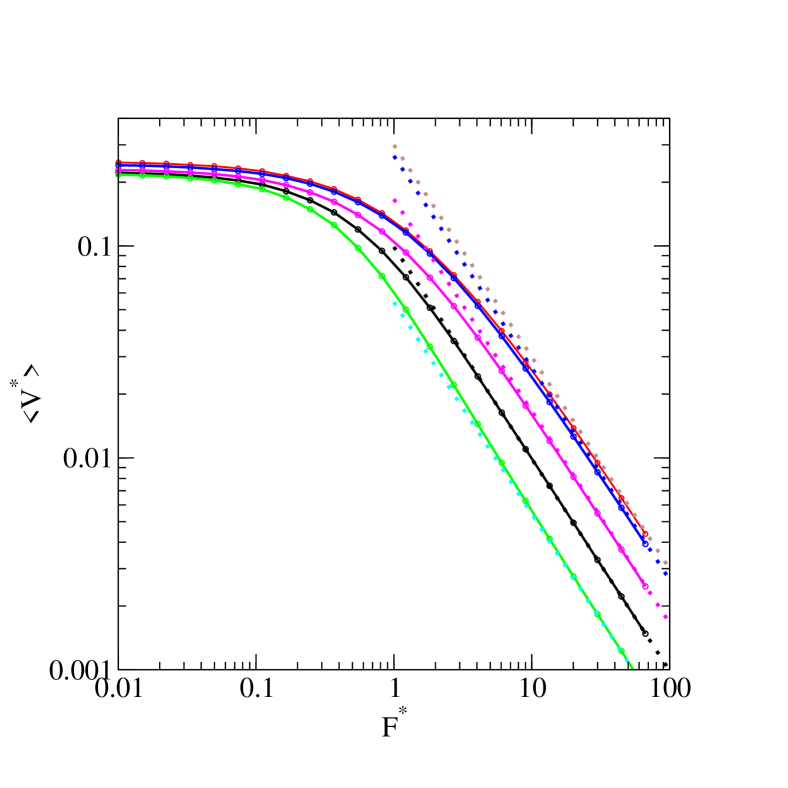
Figure 2: (Color online) Log-Log plot of the dimensionless mean velocity $\langle V^{*}\rangle$ of an asymmetric granular piston versus the dimensionless friction force $F$: $\alpha_{+}=1$, $\alpha_{-}=0$, with different mass ratio $M/m=1,2,5,10,20$. The dashed curves correspond to the analytical expression of the large friction model.

We performed numerical simulations of the Boltzmann-Lorentz equation using the Gillepsie method TV06 for different mass ratios and for a large range of dry friction. The algorithm generates collision events separated by exponentially distributed waiting intervals. Specifically, the probability that no event (collision) occurs in the time interval $(0,\Delta t)$ is given by

$$P(\Delta t)=\exp\left(-\rho\int_{0}^{\Delta t}\nu(t^{\prime})dt^{\prime}\right)$$ (10)

In the present application the mean collision flux $\rho\nu(t)$ is time dependent as the piston decelerates between collisions. A collision time, $\Delta t$, is generated by solving (numerically) the implicit equation

$$\ln(\xi)=-\rho\int_{0}^{\Delta t}\nu(t^{\prime})dt^{\prime}$$ (11)

where $0<\xi<1$ is a uniformly distributed random number. The system time is incremented by $\Delta t$ and the collision is performed by sampling a velocity of the colliding bath particle using the imposed velocity distribution $\phi(v)$ and updating the piston’s velocity using the collision rule Eq. (3). Full details can be found in TV06 .

Figure 2 shows a log-log plot of the mean velocity of an asymmetric piston ($\alpha_{+}=1$, $\alpha_{-}=0$) as a function of the dimensionless dry friction $F^{*}$ for different mass ratios $M/m=1,2,10,20$. We observe two scaling regimes: at low dimensionless friction force $F^{*}$ the dimensionless mean velocity depends weakly on $F^{*}$, whereas in the high-friction limit $F^{*}>1$, $<V^{*}>$ decays as $F^{*-1}$.

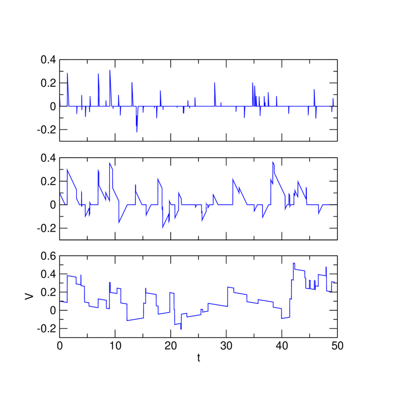
Figure 3: Dimensionless velocity, $V^{*}$, as a function of the reduced time $t^{*}=\rho L\nu(0)t$ for $F^{*}=1.0,0.1,0.01$ top to bottom. $\mu=10$.

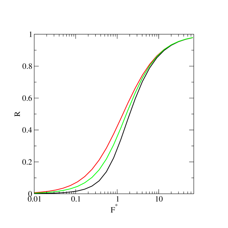
Figure 4: (Color online) Fraction of collisions occurring when the piston is at rest over the number of collisions for different masses. From left to right: $M=2,5,20$.

Useful insight can be obtained by observing the dynamics for different values of $F^{*}$: See Figure 3. For $F^{*}=1.0$ the motor decelerates rapidly after each collision until it comes to rest. It remains motionless until it is struck by another bath particle. For the smallest value, $F^{*}=0.01$, the deceleration is weak and the piston is always in motion. The case $F^{*}=0.1$ is an intermediate case.

We have also monitored the ratio $R$, of the number of collisions occurring when the piston is at rest to the total number collisions. Figure 4 shows $R$ as a function of $\Gamma_{s}$ for $M/m=1,2,10,20$. As $R$ approaches one the dynamics consists of a series of independent displacements, each followed by a period of rest before the next collision with a bath particle.

IV Time scale analysis

As we will show, the behavior of the system is governed by the relative values of the mean collision time and the mean stopping time. The mean inter-collision time between bath particles and the piston

$$\tau_{c}\simeq\frac{1}{\rho L\nu(0)}$$ (12)

is $\tau_{c}\simeq\sqrt{\frac{\pi m}{2T}}\frac{1}{\rho L}$ for a Gaussian bath distribution, and the mean stopping time with friction present, $\tau_{s}=\frac{M\overline{V}}{F}$ where $\overline{V}$ is the average velocity after a collision. When the dimensionless friction $F^{*}$ is small, $\overline{V^{*}}\sim(\alpha_{+}-\alpha_{-})$, while for $F^{*}>>1$, $\overline{V^{*}}\sim\frac{m}{M}(\alpha_{+}-\alpha_{-})$, which gives

$$\frac{\tau_{s}}{\tau_{c}}\sim\frac{\alpha_{+}-\alpha_{-}}{F^{*}}\left\{\begin{array}[]{cc}1,&F^{*}>>1\\ \frac{M}{m},&F^{*}<<1\end{array}\right.$$ (13)

This behavior is illustrated in Fig. 3, where one observes that $\tau_{s}<<\tau_{c}$ for $F^{*}=10$, whereas $\tau_{s}>>\tau_{c}$ for $F^{*}=0.1$

Whenever the dynamics consists of successive slip-stick motions, the velocity distribution function of the piston contains a regular part and a delta singularity at $V^{*}=0$ (where $V^{*}=v\sqrt{m/T}$ is the dimensionless velocity) corresponding to the situation where the piston is at rest for a finite time before the next collision with a bath particle:

$$f(V^{*})=\gamma f_{R}(V^{*})+(1-\gamma)\delta(V^{*})$$ (14)

where $\int dV^{*}f_{R}^{*}(V^{*})=1$ and $\gamma$ is a constant that can be determined from conservation of the probability current at $V^{*}=0$Touchette2010 :

$$(1-\gamma)\int_{-\infty}^{\infty}dv^{*}|v^{*}|\phi(v^{*})=2\gamma f_{R}^{*}(0)\frac{F^{*}}{\mu}$$ (15)

giving

$$\gamma^{-1}=1+2C\frac{F^{*}}{\mu}$$ (16)

with $C=2f_{R}^{*}(0)/\int_{-\infty}^{\infty}dy|y|\phi(y)$ is a numerical constant.

When $\tau_{c}>>\tau_{s}$ the frictional force stops the piston before the next collision, and the motor essentially evolves by following a sequence of stick-slip motions. Most of the time, the piston is at rest and the singular contribution is dominant, $\gamma\simeq 1/F^{*}$. This regime can be described by the independent kick model introduced below.

Conversely, when $\tau_{c}<<\tau_{s}$, collisions are so frequent that sliding dominates the piston dynamics. For all practical purposes, the piston never stops or stops for infinitesimal durations and $(1-\gamma)\simeq F^{*}$. In this case, the dynamics is well described by a Fokker-Planck equation for $M/m>>1$.

V Independent Kick model

When the friction force is large, the stopping time $\tau_{s}$ is much shorter than the mean time between collisions $\tau_{c}$. The piston dynamics is then a sequence of uncorrelated kicks immediately followed by a decelerated motion that is stopped before a next collision with a particle bath. The mean velocity is the average over all collisions.

$$\langle V\rangle=\rho L\int_{-\infty}^{\infty}dv|v|\phi(v)\int_{0}^{\tau}V(t)dt$$ (17)

where $V(t)=V_{0}-\frac{F\sigma(V_{0})}{M}t$, $\tau=\frac{|V_{0}|M}{F}$ and $V_{0}$ is the velocity after a collision, which is given by

$$V_{0}=\frac{(1+\alpha_{+})v}{1+\mu}\mbox{\rm\hskip 8.5359pt for }v>0$$ (18)

and

$$V_{0}=\frac{(1+\alpha_{-})v}{1+\mu}\mbox{\rm\hskip 8.5359ptfor }v<0$$ (19)

Integrating over time, one obtains

$$\langle V\rangle=\frac{M\rho L((1+\alpha_{+})^{2}-(1+\alpha_{-})^{2})}{2F(1+\mu)^{2}}\int_{0}^{\infty}dvv^{3}\phi(v)$$ (20)

where we have assumed that $\phi(v)$ is symmetric. With this assumption the sign of the motor effect is independent of the form of the bath velocity distribution. For a Gaussian bath distribution, the dimensionless mean velocity $<V^{*}>$ is given explicitly by

$$\langle V^{*}\rangle=\frac{((1+\alpha_{+})^{2}-(1+\alpha_{-})^{2})\mu}{2F^{*}(1+\mu)^{2}}\sqrt{\frac{2}{\pi}}$$ (21)

A second quantity of interest is the integral of the velocity distribution (obtained from Eq. (17) by setting $V=1$).

$$I_{f} =\rho L\int_{0}^{\infty}dvv^{2}\frac{|V_{0}|M}{F}\phi(v)$$

$$=\frac{\rho L(2+\alpha_{+}+\alpha_{-})M}{F(1+\mu)}\int_{0}^{\infty}dvv^{2}\phi(v)$$ (22)

For a Gaussian bath distribution, one has

$$I_{f}=\frac{(2+\alpha_{+}+\alpha_{-})\mu}{2F^{*}(1+\mu)}$$ (23)

This quantity corresponds to the value of $\gamma$ in the limit of large friction (or small ratio $\tau_{s}/\tau_{c}$). Figure 5 shows the $\delta(V^{*})$-contribution of $f(V^{*})$, $1-\gamma$ for two mass ratios $M/m=10,20$. The exact expression of the kick model Eq. (23) (dotted curves) underestimates the $\delta(V^{*})$-contribution of $f(V^{*})$. The dot-dashed curves correspond to the exact expression, Eq. (16), where $C$ is calculated by performing an exact asymptotic expansion of Eq. (V) and matching with the independent kick model Eq. (16). In this case a better agreement with simulations for small $F^{*}$ is observed. The remaining small excess is due to the fact $C$ is set to a constant, but in reality depends slightly on $F^{*}$.

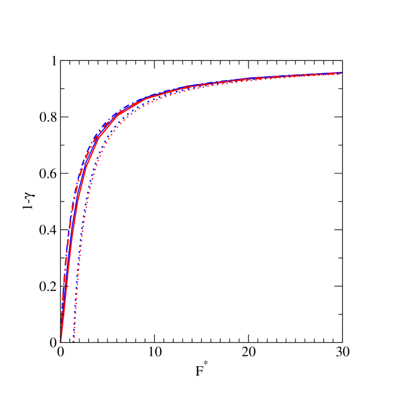
Figure 5: (Color online) $\delta(V^{*})$-contribution of $f(V^{*})$, $1-\gamma$, of an asymmetric granular piston versus $F^{*}$: $\alpha_{+}=1$, $\alpha_{-}=0$, for $M/m=10,20$. The dotted curves correspond to the analytical expression of the kick model and the dot-dashed curves to Eq. 16 where $C$ is calculated from the exact expression in the high friction limit.

The characteristic function can be also calculated

$$\langle e^{ikV}\rangle=\rho L\int_{-\infty}^{\infty}dv|v|\phi(v)\int_{0}^{\tau}e^{ikV(t)}dt$$ (24)

Integrating over time, one obtains

$$\langle e^{ikV}\rangle =\frac{\rho LM}{ikF}\int_{0}^{\infty}dvv\phi(v)$$

$$\left[\exp\left(\frac{ik(1+\alpha_{+})v}{1+\mu}\right)-\exp\left(\frac{-ik(1+\alpha_{-})v}{1+\mu}\right)\right]$$ (25)

Taking the inverse Fourier transform, one infers the velocity distribution $f_{R}(V)$

$$\gamma f_{R}(V) =\frac{\mu\rho T}{F}\left[\theta(V)\int_{\frac{(1+\mu)V}{1+\alpha_{+}}}^{\infty}dv|v|\phi\left(v\right)\right.$$

$$\left.+\theta(-V)\int^{\frac{(1+\mu)V}{1+\alpha_{-}}}_{-\infty}dv|v|\phi\left(v\right)\right]$$ (26)

Note that the regular velocity distribution $f_{R}(V)$ is continuous at $V=0$. For a Gaussian bath distribution, the dimensionless velocity distribution is then given by

$$\gamma f_{R}(V^{*}) =\frac{\mu}{F^{*}}\sqrt{\frac{1}{2\pi}}\left[\theta(V)\exp\left(-\frac{(1+\mu)^{2}V^{*2}}{2(1+\alpha_{+})^{2}}\right)\right.$$

$$\left.+\theta(-V^{*})\exp\left(-\frac{(1+\mu)^{2}V^{*2}}{2(1+\alpha_{-})^{2}}\right)\right]$$ (27)

Figure 6: (Color online) Dimensionless Velocity distributions $\gamma f(V^{*})$ for various dimensionless friction forces $F^{*}=2.72,6,05,6.6,9.02,13,6,20.09,30.0,44.7,66.7$ (From top to bottom).

Figure 7: (Color online) Rescaled velocity distributions $F^{*}\gamma f(V^{*})$ for the same values of $F^{*}$ as in Fig. 6 but in reverse order.

Velocity distributions are displayed in Fig.6 for different values of the solid friction. As expected the amplitude decreases as this quantity increases. Rescaled distributions $F^{*}f_{R}(V^{*})$ versus $V^{*}$ are shown in Fig. 7 where one observes that for $F^{*}>2$, curves converge towards the exact result, Eq. (V).

VI The Brownian limit and the Fokker-Planck equation

We now consider the opposite limit when the stopping time $\tau_{s}$ is much larger than the mean time between bath collisions $\tau_{c}$. For homogeneous granular motors where the mean velocity goes to zero in the Brownian limit Brey1999 ; Cleuren2007 , a standard Kramers-Moyal (KM) expansion of the BL integral operator leads to the Fokker-Planck differential operator. For heterogeneous granular motors, where the mean velocity remains finite and independent of the mass ratio in the Brownian limit, some caution is needed: The perturbative expansion must be performed around the non-zero mean velocity (rather than around zero)Talbot2011 . Finite mass corrections, however, cannot be easily included.

The approach we proposed in PhysRevLett.107.138001 consists of reexpressing the BL operator as a complete series expansion in terms of the derivatives of the velocity distribution function. Applying the same method to the piston we have, e.g.

$$f\left(V-\frac{1+\alpha_{+}}{1+\mu}y\right)=\sum_{n=0}^{\infty}\left(\frac{1+\alpha_{+}}{1+\mu}\right)^{n}\frac{(-y)^{n}}{n!}\frac{\partial^{n}f(V)}{\partial V^{n}}$$ (28)

with similar expressions for $\phi(V+y-\frac{1+\alpha_{+}}{1+\mu}y)$, $f(V+\frac{1+\alpha_{-}}{1+\mu}y)$ and $\phi(V-y+\frac{1+\alpha_{-}}{1+\mu}y)$. Inserting in the BL equation (II) allows us to write the collision operator as

$$J[f,\phi]=\sum_{n=1}^{\infty}\frac{1}{n!\mu^{n}}\frac{\partial^{n}(g_{n}(V)f(V))}{\partial V^{n}}$$ (29)

where we have used the fact that the zero order terms of the expansion cancel the destruction term and where we have introduced

$$g_{n}(V) =\rho L\int_{0}^{\infty}dy\;y\left[\left(-\mu\frac{1+\alpha_{+}}{1+\mu}\right)^{n}\phi(V+y)+\right.$$

$$\left.\left(\mu\frac{1+\alpha_{-}}{1+\mu}\right)^{n}\phi(V-y)\right]$$ (30)

The functions $g_{n}(V)$ can be obtained from the generating function

$$g(V,a)=\rho L\int_{0}^{\infty}dyy\left[\exp\left(\frac{-(1+\alpha_{+})\mu ya}{1+\mu}\right)\right.\phi(V+y)$$

$$+\left.\exp\left(\frac{(1+\alpha_{-})\mu ya}{1+\mu}\right)\phi(V-y)\right]$$ (31)

Truncating the BL operator, Eq. (29), at second-order and adding the dry friction leads to the following Fokker-Planck equation

$$\frac{\partial f(V,t)}{\partial t} =\frac{1}{M}\frac{\partial}{\partial V}\left[(F\sigma(V)+mg_{1}(V))f(V,t)\right]$$

$$+\frac{1}{2M^{2}}\frac{\partial^{2}}{\partial V^{2}}[m^{2}g_{2}(V)f(V,t)]=0$$ (32)

in which all finite-mass corrections are incorporated, and where deviations from a Gaussian distribution are present for large finite masses. Recalling that the $g_{n}(V)$ are proportional to $\rho$, we see that for a given dry friction $F$, increasing the bath density reduces the effect of friction. The corresponding Langevin equation Gardiner_2009 features a motor force with a non-linear dependence on $V$ and a colored noise.

$$M\frac{dV}{dt}=-F\sigma(V)-mg_{1}(V)+m\sqrt{g_{2}(V)}\eta(t)$$ (33)

where $\eta(t)$ is a white Gaussian noise, where $\langle\eta(t)\rangle=0$ and $\langle\eta(t)\eta(t^{\prime})\rangle=\delta(t-t^{\prime})$

The steady state solution of Eq. (VI) is

$$f(V)=\frac{C_{f}}{g_{2}(V)}\exp\left[-2M\int_{0}^{V}du\;\left(\frac{mg_{1}(u)+F\sigma(u)}{m^{2}g_{2}(u)}\right)\right]$$ (34)

where $C_{f}$ is obtained from the normalization condition $\int dVf(V)=1$. This result clearly shows that, even in the absence of friction, the velocity distribution is non-Gaussian for finite mass ratios.

In the Brownian limit $g_{1}(V)\sim g^{\prime}_{1}(\tilde{V})(V-\tilde{V})$ and $g_{2}(V)=2T_{g}/mg^{\prime}_{1}(\tilde{V})$, where $T_{g}$ (the granular temperature of the piston which is lower than the bath temperature, $T$) and $\tilde{V}$ are given by the Kramers-Moyal expansion (Eqs. (6) and (8) in Ref. PhysRevE.82.011135 ). (Physically, $\tilde{V}$ is the exact steady state drift velocity of a piston in the Brownian limit in the absence of friction). This finally gives a stationary distribution, at the lowest order in $m/M$,

$$f(V)=C\exp\left(-\frac{M(V-\tilde{V})^{2}}{2T_{g}}-\frac{\mu F|V|}{g_{1}^{\prime}(\tilde{V})T_{g}}\right)$$ (35)

where $C$ is the normalization constant. Whereas one observes a Gaussian decay of the velocity distribution at large velocity, $f(V)$ decreases exponentially for small and intermediate velocities, due to friction JPSJ.73.2037 ; Chaudhury2008 ; Touchette2010 .

VII Static Friction

Our analysis has so far been restricted to dynamic dry friction that produces a constant retarding force on a moving piston. A stationary piston acquires a non-zero velocity following a collision with a bath particle, no matter how slowly the latter is moving. In reality, static friction will also be present and this will prevent the piston from moving unless it is struck by a sufficiently fast moving bath particle. To model this effect correctly using a coefficient of static friction we would need to know the time-dependent force acting on a stationary piston during a collision with a bath particle. If this force exceeds the force due to static friction, the piston starts to move. In the present model, however, the collisions are assumed to be instantaneous. Therefore, we represent static friction in an approximate way, by introducing a threshold impulse $I_{m}$ so that the piston is only set into motion if $|I_{\pm}|>I_{m}$.

$$V^{\prime}=\left\{\begin{array}[]{rl}\displaystyle\frac{m}{m+M}(1+\alpha_{+})v-\frac{I_{m}}{m+M}&\mbox{ if $v>\frac{I_{m}}{m(1+\alpha_{+})}$}\\ \displaystyle\frac{m}{m+M}(1+\alpha_{-})v+\frac{I_{m}}{m+M}&\mbox{ if $v<-\frac{I_{m}}{m(1+\alpha_{-})}$}\\ \displaystyle 0&\mbox{ otherwise}\end{array}\right.$$ (36)

This implies that a colliding bath particle must be moving faster than

$$v^{\pm}_{m}=\pm\frac{I_{m}}{m(1+\alpha_{\pm})}$$ (37)

to set a stationary piston into motion. Let us introduce the dimensionless threshold impulse

$$I^{*}_{m}=\frac{I_{m}}{\sqrt{mT}}$$ (38)

the effect of static friction consists of adding a singular contribution to the velocity distribution and of weakening the motor effect.

When the time scale ratio $\tau_{s}/\tau_{c}>>1$, it is easy to generalize the independent kick model by adding the static friction. The drift velocity is given by

$$\langle V\rangle=\rho L\int_{v^{+}_{m}}^{\infty}dvv\phi(v)\int_{0}^{\tau}dtV(t)$$

$$+\rho L\int^{v^{-}_{m}}_{-\infty}dvv\phi(v)\int_{0}^{\tau}dtV(t)$$ (39)

where $V(t)=V_{0}-\frac{F\sigma(V)}{M}t$, $\tau=\frac{M|V_{0}|}{F}$ and $V_{0}$ is given by Eq. (36).

Integrating over time, one obtains the following expression

$$\langle V\rangle=\frac{M\rho L}{2F(1+\mu)^{2}}\left((1+\alpha_{+})^{2}\int_{v^{+}_{m}}^{\infty}dv\,v(v-v^{+}_{m})^{2}\phi(v)\right.$$

$$\left.-(1+\alpha_{-})^{2}\int_{-\infty}^{v^{-}_{m}}dv\,|v|(v^{-}_{m}-v)^{2}\phi(v)\right)$$ (40)

For a Gaussian bath velocity distribution, the dimensionless mean velocity is given by

$$\langle V^{*}\rangle=\frac{\mu}{2F^{*}(1+\mu)^{2}}[h(I^{*}_{m},\alpha_{+})-h(I^{*}_{m},\alpha_{-})]$$ (41)

with

$$h(I^{*}_{m},\alpha)=(1+\alpha)^{2}\sqrt{\frac{2}{\pi}}\exp\left(-\frac{I_{m}^{*2}}{2(1+\alpha)^{2}}\right)$$

$$-(1+\alpha)I_{m}^{*}erfc\left(\frac{I_{m}^{*}}{\sqrt{2}(1+\alpha)}\right)$$ (42)

that correctly reduces to Eq. (21) if $I^{*}_{m}=0$.

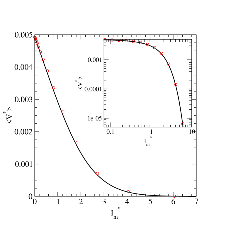
Figure 8: (Color online) Dimensionless mean velocity of an asymmetric granular piston of mass ratio $M/m=10$ with a friction force $F^{*}=20.01$: $\alpha_{+}=1$, $\alpha_{-}=0$, versus the threshold impulse. The circles correspond to the simulation results with the static friction and the solid lines show the theoretical result, Eq. (41).

Fig. 8 shows that the theoretical result is in good agreement with numerical simulations of the Boltzmann-Lorentz equation with static and dynamic friction.

Developing Eq. (41) as a power series about $I^{*}_{m}=0$, we obtain

$$\langle V^{*}\rangle=\frac{\mu}{2F^{*}(1+\mu)^{2}}(\alpha_{+}-\alpha_{-})\left[(2+\alpha_{+}+\alpha_{-})\sqrt{\frac{2}{\pi}}\right.$$

$$\left.-I^{*}_{m}+O(I^{*4}_{m})\right]$$ (43)

We note the absence of terms in $I^{*2}_{m}$ and $I^{*3}_{m}$ and from Fig. 8 we see that the mean velocity increases linearly for $I^{*}_{m}<2$. Furthermore, a non-zero impulse threshold means that, in additon to the simple scaling behaviour ($\langle V\rangle\sim T^{3/2}$) with only dynamic friction present, a sub-dominant term appears:

$$\langle V\rangle\propto(\alpha_{+}-\alpha_{-})\left[(2+\alpha_{+}+\alpha_{-})\sqrt{\frac{2}{\pi}}T^{3/2}-\frac{I_{m}}{\sqrt{m}}T\right]$$ (44)

The asymptotic behavior for large values of $I^{*}_{m}$ is

$$\langle V^{*}\rangle =\frac{\mu}{2F^{*}(1+\mu)^{2}}\frac{1}{I^{*2}_{m}}\sqrt{\frac{2}{\pi}}\left[(1+\alpha_{+})^{4}\exp(-\frac{I^{*2}_{m}}{2(1+\alpha_{+})^{2}})\right.$$

$$\left.-(1+\alpha_{-})^{4}\exp(-\frac{I^{*2}_{m}}{2(1+\alpha_{-})^{2}})\right]$$ (45)

In this limit only fast-moving bath particles, which are few since they correspond to the tails of the bath velocity distribution, can actuate a stationary piston. Therefore, the motor effect vanishes. The integral of the velocity distribution is

$$I_{f}=\frac{ML\rho}{(1+\mu)F}\left[(1+\alpha_{+})\int_{v^{+}_{m}}^{\infty}dvv(v-v^{+}_{m})\phi(v)\right.$$

$$\left.+(1+\alpha_{-})\int^{v^{-}_{m}}_{-\infty}dv|v|(v^{-}_{m}-v)\phi(v)\right]$$ (46)

that, for a Gaussian bath velocity distribution, gives

$$I_{f}= \frac{\mu}{(1+\mu)F^{*}}\left[(1+\alpha_{+})erfc\left(\frac{I^{*}_{m}}{\sqrt{2}(1+\alpha_{+})}\right)\right.$$

$$\left.+(1+\alpha_{-})erfc\left(\frac{I^{*}_{m}}{\sqrt{2}(1+\alpha_{-})}\right)\right]$$ (47)

that goes rapidly to zero for $I^{*}_{m}>2$.

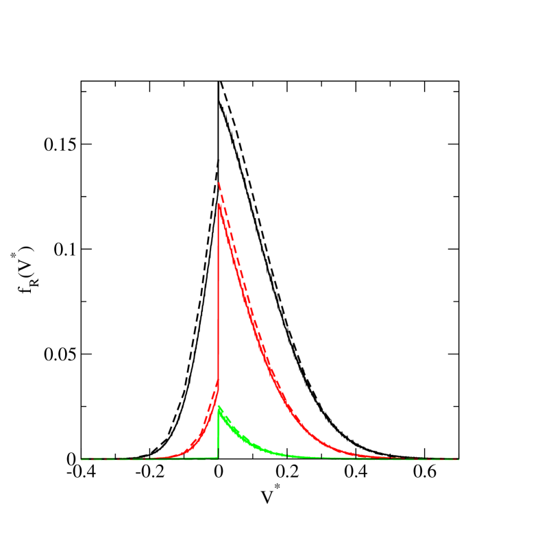
Figure 9: (Color online) Dimensionless velocity distributions of an asymmetric granular piston of mass ratio $M/m=10$ a friction force $F^{*}=20.01$: $\alpha_{+}=1$, $\alpha_{-}=0$, with different static frictions $I_{m}^{*}=0.82,1.82,4.06$. The dashed curves correspond to the analytical expression of the independent kick model with the static and dynamic frictions, Eq. (VII).

Finally, the characteristic function $\langle e^{ikV}\rangle$ is given by

$$\langle e^{ikV}\rangle=\frac{\rho ML}{F}\left[\int_{v^{+}_{m}}^{\infty}dv|v|\phi(v)\frac{e^{i\frac{1+\alpha_{+}}{1+\mu}k(v-v^{+}_{m})}-1}{ik}\right.$$

$$\left.+\int^{v^{-}_{m}}_{-\infty}dv|v|\phi(v)\frac{e^{i\frac{1+\alpha_{-}}{1+\mu}k(v-v^{-}_{m})}-1}{ik}\right]$$ (48)

Taking the inverse Fourier transform one obtains the velocity distribution

$$\gamma f_{R}(V)=\frac{\rho ML}{F}\left[\theta(V)\int_{\frac{I^{*}_{m}}{1+\alpha_{+}}+\frac{1+\mu}{1+\alpha_{+}}V}^{\infty}dv|v|\phi(v)\right.$$

$$+\theta(-V)\left.\int^{\frac{-I^{*}_{m}}{1+\alpha_{-}}+\frac{1+\mu}{1+\alpha_{-}}V}_{-\infty}dv|v|\phi(v)\right]$$ (49)

For a Gaussian distribution, the dimensionless velocity distribution is expressed as

$$\gamma f_{R}(V^{*})=\frac{\mu}{F^{*}}\sqrt{\frac{1}{2\pi}}\left[\theta(V)\exp\left(-\frac{\left({I_{m}^{*}+(1+\mu)V^{*}}\right)^{2}}{2(1+\alpha_{+})^{2}}\right)\right.$$

$$+\left.\theta(-V)\exp\left(-\frac{\left({-I_{m}^{*}+(1+\mu)V^{*}}\right)^{2}}{2(1+\alpha_{-})^{2}}\right)\right]$$ (50)

We see that static friction has a dramatic qualitative effect on the regular velocity distribution in the sense that it is discontinuous at $V^{*}=0$, a feature not present for $I^{*}_{m}=0$.

$$\gamma f_{R}(0+)-\gamma f_{R}(0-)=\frac{\mu}{F^{*}}\sqrt{\frac{1}{2\pi}}\left[\exp\left(-\frac{I_{m}^{*2}}{2(1+\alpha_{+})^{2}}\right)\right.$$

$$\left.-\exp\left(-\frac{I_{m}^{*2}}{2(1+\alpha_{-})^{2}}\right)\right]$$ (51)

Figure 9 shows velocity distributions when $F^{*}=20.01$, $M/m=10$, and for different values of the impulse threshold (full curves). The independent kick model incorporating dynamic and static friction provides an accurate description of the kinetic properties of the Boltzmann-Lorentz equation. As expected, one observes a finite discontinuity of the velocity distribution at $V=0$. Negative piston velocities occur less frequently than positive ones due to the low efficiency of bath collisions on the right side of the piston ($\alpha_{-}=0$) and the momentum threshold of the static friction. As the static friction increases, motion of the piston to the left is reduced more rapidly than motion to the right.

VIII Conclusion

We have considered the effect of dynamic and static friction on the kinetics of a granular asymmetric piston. When only dynamic friction is present, the mean velocity exhibits two scaling regimes depending on the strength of the friction force. In the high friction limit, the Boltzmann-Lorentz equation is asymptotically described by a solvable independent kick model. Conversely, when the friction is small, and if the mass ratio is large, the model can be mapped to Fokker-Planck equation, for which exact results can be also obtained. When static, as well as dynamic, friction is present the mean piston velocity initially decreases linearly with the threshold impulse, while for larger values of this parameter the motor effect is rapidly suppressed, decreasing in a Gaussian fashion.

Further investigation could consider collective effects of motor assemblies observed in biological systems Howard2009 ; PhysRevLett.104.248102 ; PhysRevLett.106.068101 or dense granular systems with active particles PhysRevE.81.061916 ; PhysRevLett.101.268101 ; PhysRevLett.105.098001 ; Baskaran2010 .

References

- (1) H. B. Callen, “Thermodynamics,” (John Wiley and Sons, Inc., 1960) Chap. Equilibrium with internal adiabatic constrains, Appendix C
- (2) J. Piasecki and C. Gruber, Physica A 265, 463 (1999)
- (3) C. Gruber and J. Piasecki, Physica A 268, 412 (1999)
- (4) C. Gruber, S. Pache, and A. Lesne, J. Stat. Phys. 108, 669 (2002)
- (5) C. Gruber, S. Pache, and A. Lesne, J. Stat. Phys. 112, 1177 (2003)
- (6) C. Gruber and A. Lesne, in Encyclopedia of Mathematical Physics, edited by J.-P. Françoise, G. L. Naber, , and T. S. Tsun (Academic Press, Oxford, 2006) p. 160
- (7) R. Brito, M. J. Renne, and C. V. den Broeck, Europhys. Lett. 70, 29 (2005)
- (8) J. J. Brey and N. Khalil, Phys. Rev. E 82, 051301 (2010)
- (9) G. Costantini, U. M. B. Marconi, and A. Puglisi, Phys. Rev. E 75, 061124 (2007)
- (10) G. Costantini, U. Marini Bettolo Marconi, and A. Puglisi, Europhys. Lett. 82, 50008 (2008)
- (11) J. Talbot, A. Burdeau, and P. Viot, Phys. Rev. E 82, 011135 (2010)
- (12) P. Eshuis, K. van der Weele, D. Lohse, and D. van der Meer, Phys. Rev. Lett. 104, 248001 (2010)
- (13) M. Smoluchowski, Physik. Zeitschr 13, 1069 (1912)
- (14) The Feynman Lectures on Physics, edited by R. L. R.P. Feynman and M. Sands (Addison-Wesley, 1963)
- (15) P. Reimann, Phys. Rep. 361, 57 (2002)
- (16) F. Jülicher, A. Ajdari, and J. Prost, Rev. Mod. Phys. 69, 1269 (1997)
- (17) van den Broek, M., Eichhorn, R., and Van den Broeck, C., EPL 86, 30002 (2009)
- (18) B. Cleuren and C. V. den Broeck, Europhys. Lett. 77, 50003 (2007)
- (19) B. Cleuren and R. Eichhorn, J. Stat. Mech. 2008, P10011 (2008)
- (20) G. Costantini, A. Puglisi, and U. Marconi, Eur. Phys. J. Special Topics 179, 197 (2009)
- (21) P. G. d. Gennes, J. Stat. Phys. 119, 953 (2005)
- (22) H. Hayakawa, Physica D 205, 48 (2005)
- (23) A. Kawarada and H. Hayakawa, J. Phys. Soc. Jpn. 73, 2037 (2004)
- (24) A. M. Menzel and N. Goldenfeld, Phys. Rev. E 84, 011122 (Jul 2011)
- (25) A. Mauger, Physica A 367, 129 (2006)
- (26) H. Touchette, E. V. der Straeten, and W. Just, J. Phys. A: Math. Gen. 43, 445002 (2010)
- (27) A. Baule, E. G. D. Cohen, and H. Touchette, J. Phys. A: Math. Gen. 43, 025003 (2010)
- (28) A. Baule, H. Touchette, and E. G. D. Cohen, Nonlinearity 24, 351 (2011)
- (29) A. Buguin, F. Brochard, and P.-G. de Gennes, Eur. Phys. J. E 19, 31 (2006)
- (30) M. K. Chaudhury and S. Mettu, Langmuir 24, 6128 (2008)
- (31) P. S. Goohpattader, S. Mettu, and M. K. Chaudhury, Langmuir 25, 9969 (2009)
- (32) S. Mettu and M. K. Chaudhury, Langmuir 26, 8131 (2010)
- (33) J. Talbot, R. D. Wildman, and P. Viot, Phys. Rev. Lett. 107, 138001 (2011)
- (34) J. Piasecki, J. Talbot, and P. Viot, Phys. Rev. E 75, 051307 (2007)
- (35) J. Talbot and P. Viot, J. Phys. A: Math. Gen. 39, 10947 (2006)
- (36) J. J. Brey, J. W. Dufty, and A. Santos, J. Stat. Phys. 97, 281 (1999)
- (37) J. Talbot, A. Burdeau, and P. Viot, J. Stat. Mech. 2011, P03009 (2011)
- (38) C. W. Gardiner, Stochastic Methods: A Handbook for the Natural and Social Sciences (Springer, 2009)
- (39) J. Howard, Annual Review of Biophysics 38, 217 (2009)
- (40) T. Guérin, J. Prost, and J.-F. Joanny, Phys. Rev. Lett. 104, 248102 (2010)
- (41) T. Guérin, J. Prost, and J.-F. Joanny, Phys. Rev. Lett. 106, 068101 (2011)
- (42) S. Mishra, A. Baskaran, and M. C. Marchetti, Phys. Rev. E 81, 061916 (2010)
- (43) A. Baskaran and M. C. Marchetti, Phys. Rev. Lett. 101, 268101 (2008)
- (44) J. Deseigne, O. Dauchot, and H. Chaté, Phys. Rev. Lett. 105, 098001 (Aug 2010)
- (45) A. Baskaran and M. C. Marchetti, J. Stat. Mech. 2010, P04019 (2010)