Le Chatelier principle in replicator dynamics

Abstract

The Le Chatelier principle states that physical equilibria are not only stable, but they also resist external perturbations via short-time negative-feedback mechanisms: a perturbation induces processes tending to diminish its results. The principle has deep roots, e.g., in thermodynamics it is closely related to the second law and the positivity of the entropy production. Here we study the applicability of the Le Chatelier principle to evolutionary game theory, i.e., to perturbations of a Nash equilibrium within the replicator dynamics. We show that the principle can be reformulated as a majorization relation. This defines a stability notion that generalizes the concept of evolutionary stability. We determine criteria for a Nash equilibrium to satisfy the Le Chatelier principle and relate them to mutualistic interactions (game-theoretical anticoordination) showing in which sense mutualistic replicators can be more stable than (say) competing ones. There are globally stable Nash equilibria, where the Le Chatelier principle is violated even locally: in contrast to the thermodynamic equilibrium a Nash equilibrium can amplify small perturbations, though both this type of equilibria satisfy the detailed balance condition.

I Introduction

An external influence disturbing an equilibrium state of a system induces processes tending to diminish the results of the disturbance. This is the qualitative content of the principle formulated by Le Chatelier for chemical reactions edu . Earlier statements of the principle are reviewed in phi . Braun related the principle to the second law and extended it to general thermodynamic equilibria landau ; gilmore . In contrast to the second law, the Le Chatelier principle is more operational and more intuitive; hence it became the main tool for predicting the response of physical and chemical equilibrium edu ; landau ; gilmore . Applications of the principle go well beyond physics and chemistry: in economics it is used for the analysis of price equilibrium econo ; in ecology for explaining qualitatively the ecosystems growth nature ; jorge , and also for quantifying the threshold of allowed influences of civilization on the environment gorshkov . The principle gave rise to the concept of homeostasis, a state of an organism or construction that is stable due to compensatory mechanisms phi .

The issue of stability is also central to population dynamics and ecology: to a large extent these disciplines emerged and developed around various aspects of the stability notion and its relations to diversity, productivity, complexity etc svi ; see ives for a recent review. The question of understanding pertinent forms of stability is presently more pending than ever in face of various environmental issues and global changes.

Our purpose here is to develop a formalization of the Le Chatelier principle for a game-theoretical population dynamics and to show that it leads to a notion of stability that allows to make new predictions. In particular, the Le Chatelier principle differs from the asymptotic stability arnold , where—once a (small) perturbation is over—the equilibrium is recovered after a sufficiently large time (relaxation) . It is however not excluded that in the course of relaxation the perturbation will be transiently amplified, a scenario forbidden by the Le Chatelier principle. While the asymptotic stability indicates on long-time negative feedback (perturbation does decay sooner or later), the principle means a short-time negative feedback.

Our setup is the the replicator dynamics, a basic description of the Evolutionary Game Theory (EGT) and population dynamics zeeman ; hofbauer ; sandholm ; svi . This dynamics originated in 1930’s as a population approach to genetics hofbauer . Later on it merged with game theory sandholm and with mathematical ecology svi . It has a wide range of applications from biology, ecology and economics hofbauer ; sandholm ; svi to physics armen_mahler and combinatorial optimization menon . EGT describes large populations of agents (humans, animals, microbes, genes) interacting via playing a game. Changes in these populations are driven either by the application of decision rules by individual agents, or by natural selection via different reproduction rates zeeman ; hofbauer ; sandholm . EGT related the Nash equilibrium of a static game to attractors of dynamics zeeman ; hofbauer ; sandholm , thereby likening the Nash equilibrium to the thermodynamic equilibrium. EGT also put forward the concept of evolutionary stability, a widely used notion related to stability with respect to invasions zeeman ; hofbauer ; sandholm .

Here we show that i) for perturbations of an asymptotically stable Nash equilibrium the Le Chatelier principle can be reformulated as a majorization relation. ii) the criterion for the principle relates to mutualistic [cooperative] interactions between agents (game-theoretical anticoordination). iii) A weaker formulation of the Le Chatelier principle, which demands that a perturbation is at least not amplified , provides a stability concept with a wider applicability than the evolutionary stability, e.g., the principle can be applied to permanent replicators that do not possess an asymptotically stable state. iv) Non-mutualistic (competitive or prey-predator) interactions can violate even the weak formulation of the principle, i.e., small perturbations over an asymptotically stable Nash equilibrium can be amplified. This is impossible for thermodynamic equilibria and shows that Nash equilibria can be endowed with positive feedback.

This paper is structured as follows: Section II introduces the Le Chatelier principle and explains its meaning: II.2 states a weaker version of the principle and shows its relations with multiple perturbations. Section III recalls the replicator dynamics and the main features of the Nash equilibrium. In particular, section III.2 explain why the notion of Nash equilibrium is indeed similar to the thermodynamic equilibrium, while section III.3 reviews the concept of evolutionary stability and relates it with the notion of mutualism as the whole. Section IV obtains the criteria of the Le Chatelier principle for the replicator dynamics. Section V studies the principle for concrete population games. The last section concludes and makes connections with previous works and ideas.

II Le Chatelier principle

II.1 The formulation

The standard formulation of the principle in equilibrium thermodynamics refers to small perturbations of extensive variables (volume, number of particles for a certain substance, etc) gilmore . The linear non-equilibrium thermodynamics formulates the principle via fluxes and forces again for small deviations from equilibrium groot ; trincher . In contrast, we need a formulation that works within the non-equilibrium statistical mechanics approach, where the basic quantities are probabilities of states satisfying certain equations of motions. Such a formulation should refer to not necessarily small perturbations of the autonomous equations of motion.

Let a system is described by a probability vector from the simplex ${\bf S}_{n}$:

$${\bf x}\in{\bf S}_{n}~{}:~{}{\bf x}^{\rm T}\equiv\{x_{k}\geq 0\}_{k=1}^{n},\qquad{\sum}_{k=1}^{n}x_{k}=1,$$ (1)

where the probabilities $x_{k}$ refer to occupation of various states in the population, and where ${\bf x}^{\rm T}$ means transposition of the column ${\bf x}$. In statistical physics the index $k$ typically refers to (free) energy levels or to phase-space cells landau . In population dynamics $k$ refers to groups of agents having certain common features (traits). The interior of ${\bf S}_{n}$ is given by $x_{k}>0$ and ${\sum}_{k=1}^{n}x_{k}=1$.

Let ${\bf x}(t)$ satisfy a continuous-time master equation:

$${\rm d}x_{i}(t)/{\rm d}t\equiv\dot{x}_{i}={\sum}_{k=1}^{n}W_{ik}[{\bf x}]x_{k},~{}{\sum}_{i=1}^{n}W_{ik}[{\bf x}]=0,$$ (2)

where $W_{i\not=k}[{\bf x}]\geq 0$ is the transition probability $k\to i$, and ${\sum}_{i=1}^{n}W_{ik}[{\bf x}]=0$ follows from ${\sum}_{k=1}^{n}x_{k}=1$. Eq. (2) is the base for non-equilibrium statistical mechanics, chemical kinetics and population dynamics kampen . $W_{i\not=k}[{\bf x}]$ may depend on ${\bf x}$ (non-linear case), as in the Boltzmann equation kampen or in the replicator equation hofbauer ; sandholm . When $W_{i\not=k}$ does not depend on ${\bf x}$ (linear case), (2) refers to the one-time probability a continuous-time Markov process .

Let ${\bf p}^{\rm T}=\{p_{k}>0\}_{k=1}^{n}$ be an asymptotically stable rest-point of (2). A sudden perturbation at time $t$ brings the system from ${\bf p}$ to some ${\bf x}(t)$ from the attraction basin of ${\bf p}$. The perturbation is quantified via ratios $\{x_{k}(t)/p_{k}\}_{k=1}^{n}$. We re-number these ratios as

$${x^{\downarrow}_{1}(t)}/{p^{\downarrow}_{1}}\,\,\geq\,\,{x^{\downarrow}_{2}(t)}/{p^{\downarrow}_{2}}\,\,\geq\,\,\ldots\,\,\geq\,\,{x^{\downarrow}_{n}(t)}/{p^{\downarrow}_{n}}.$$ (3)

Thus $x^{\downarrow}_{1}(t)$ [$x^{\downarrow}_{n}(t)$] is the largest [smallest] component of perturbation. The solution of (2) is a smooth function of time. Hence the ordering (3) holds at time $t+\epsilon$ with a small $\epsilon>0$:

$${x^{\downarrow}_{1}(t+\epsilon)}/{p^{\downarrow}_{1}}\,\geq\,{x^{\downarrow}_{2}(t+\epsilon)}/{p^{\downarrow}_{2}}\,\geq\,\ldots\,\geq\,{x^{\downarrow}_{n}(t+\epsilon)}/{p^{\downarrow}_{n}}.$$ (4)

If all inequalities in (3) are strict, the transition from (3) to (4) is obvious, since $\epsilon\to 0$ and ${\bf x}(t)$ is a continuous function. If some of them are equalities, ordering (3) is not unique, but it can be chosen such that (4) holds. Perturbations can have external origin, or be related to intrinsic noise. In the latter scenario (2) arises as a deterministic approximation to a random dynamics sandholm , so that the remnants of noise can be described as rare random perturbations.

To formulate the Le Chatelier principle gradually assume first that $n=3$. According to (3), $x_{1}$ is the strongest component of the perturbation. Short-time negative feedback means that it decays: $x^{\downarrow}_{1}(t+\epsilon)\leq x^{\downarrow}_{1}(t)$. Likewise, $x^{\downarrow}_{3}(t)$ is the smallest component of the perturbation. It may be close to zero making the corresponding group vulnerable to extinction due to intrinsic noise sandholm . The Le Chatelier principle requires negative feedback mechanisms increasing $x^{\downarrow}_{3}(t)$: $x^{\downarrow}_{3}(t+\epsilon)\geq x^{\downarrow}_{3}(t)$. Combining this with the above condition on $x^{\downarrow}_{1}(t)$ we obtain (5) for $n=3$. For $n>3$ we note that we may define the sum $x^{\downarrow}_{1}(t)+x^{\downarrow}_{2}(t)$ as the largest component of the perturbation and demand its decay in time. Likewise, $x^{\downarrow}_{n}(t)+x^{\downarrow}_{n-1}(t)$ can be taken as the smallest component demanding its non-decrease in time. Hence we come to the following formulation for the Le Chatelier principle to hold for times $t\in[0,{\cal T}]$ for perturbation ${\bf x}(t)$ ($\epsilon\to 0+$):

$${\sum}_{k=1}^{m}x^{\downarrow}_{k}(t+\epsilon)\leq{\sum}_{k=1}^{m}x^{\downarrow}_{k}(t),\quad 1\leq m\leq n,$$ (5)

with the equality for $m=n$. Taking $\epsilon\to 0$ in (5) we get:

$${\sum}_{k=1}^{m}\dot{x}^{\downarrow}_{k}(t)\leq 0,\quad 1\leq m\leq n.$$ (6)

This formulation can be presented in an equivalent form. Eqs. (5, 3, 4) imply that for any convex [$f^{\prime\prime}(y)\geq 0$] function $f(y)$ one has ruch_mead ; ruch_trio ; olkin :

$${\sum}_{k=1}^{n}p_{k}f(x_{k}(t+\epsilon)/p_{k})\leq{\sum}_{k=1}^{n}p_{k}f(x_{k}(t)/p_{k}),$$ (7)

which after taking the limit $\epsilon\to 0+$ reduces to

$${\sum}_{k=1}^{n}\dot{x}_{k}f^{\prime}(x_{k}(t)/p_{k})\leq 0,\qquad f^{\prime}(x)={\rm d}f/{\rm d}x.$$ (8)

The converse holds as well ruch_mead ; ruch_trio ; olkin : (7, 3, 4) imply (5) . Eq. (7) holds for all convex functions $f(y)$, if it holds for special classes of convex functions; see Footnote 6. For an illustration of (7) take, e.g., $f(y)=|1-y|$. Then (7) will demand time-decay of ${\sum}_{k=1}^{n}|p_{k}-x_{k}(t)|$, which is an intuitive measure of the perturbation magnitude. Many other such intuitive measures are inlcluded in (7) gorban .

Eq. (8) implies that a function $F[{\bf x}(t);f]={\sum}_{k=1}^{n}p_{k}f(x_{k}(t)/p_{k})$ monotonously decays in time to its minimum $f(1)$, which is reached for ${\bf x}={\bf p}$. Convexity of $f$ implies that $f(1)$ is both local and global minimum for $F[{\bf x}(t);f]$. In contrast to asymptotic stability, which always relates to some Lyapunov function chetaev , the Le Chatelier principle requires a specific class of Lyapunov functions; see Footnote 6 for one choice of such a class.

Conditions (3, 4, 5) amount to the definition of majorization order known in different areas of probability theory ruch_mead ; ruch_trio ; olkin ; ruch_lesche and applied to master equations in schlogl ; alberti ; michal ; menon : ${\bf x}(t)$ majorizes ${\bf x}(t+\epsilon)$ relative to ${\bf p}$

$${\bf x}(t)\,\succ_{{\bf p}}\,{\bf x}(t+\epsilon),\qquad\epsilon\to 0+.$$ (9)

Note: i) ${\bf p}\,\succ_{{\bf p}}\,{\bf x}$ leads to ${\bf x}={\bf p}$, as follows from (5) and the fact that (3) implies $1\leq{x^{\downarrow}_{1}(t)}/{p^{\downarrow}_{1}}\geq{x^{\downarrow}_{n}(t)}/{p^{\downarrow}_{n}}\leq 1$. ii) ${\bf x}(t)\,\succ_{{\bf p}}\,{\bf p}$ for any ${\bf x}(t)$. This follows from the convexity of $f(x)$ in (7) and means that being extended to long times, the Le Chatelier principle becomes equivalent to asymptotic stability of ${\bf p}$: ${\bf x}(t)\,\succ_{{\bf p}}\,{\bf x}(t+\infty)={\bf p}$. Hence one interpret (9) in terms of ”information distance” ruch_lesche : ${\bf x}(t+\epsilon)$ is closer to ${\bf p}$ than ${\bf x}(t)$.

II.2 Weak formulation of the Le Chatelier principle

When applying the Le Chatelier principle (6, 3, 4), it will prove convenient to separate the case where some of conditions (6) [or (5)] are violated, but not all of them are violated simultaneously. This will be refered to as the weak formulation of the Le Chatelier principle: although the perturbation is not diminished, it is also not amplified. The weak formulation does not imply asymptotic stability, but still it prevents strong unstabilities. If all inequalities in (6) [or in (5)] are reversed, we get perturbation amplification that is in sharp contrast to the Le Chatelier principle. The weak formulation can be applied to stable [but not asymptotically stable] rest-point.

In the stability theory one typically studies consequences of a single perturbation. It is recognized that the standard measures of stability are insufficient for treating a sequence of multiple perturbations justus . The Le Chatelier principle treats this situation, e.g. a violated weak principle would mean that a sequence of weakening perturbations may drive the system towards the boundaries of (1), where the extinction risks are sizable.

Another way of weakening the formulation (5, 6) of the Le Chatelier principle is to require only decrease of the largest component of the perturbation and increase of the smallest component: $\dot{x}^{\downarrow}_{1}\leq 0$ and $\dot{x}^{\downarrow}_{n}\geq 0$. For $n\geq 4$ this differs from (6). Likewise, a stronger [than (5,7)] formulation is also possible: one may require the relation (5, 3, 4) to hold not only for $\epsilon\to 0+$, but also for all $\epsilon>0$. Both are worth exploring, but are not at focus here.

II.3 Linear master-equation

Eqs. (7, 8) hold if in (2) $W_{ik}$ does not depend on ${\bf x}$ (linear master-equation)ruch_mead ; ruch_trio ; olkin ; ruch_lesche ; schlogl ; alberti ; michal ; gorban . For a small $\epsilon$ and arbitrary ${\bf x}(t)>0$ we write (2) as ${\bf x}(t+\epsilon)=\Pi{\bf x}(t)$, where $\Pi$ is a stochastic matrix, $\Pi_{ik}\equiv\delta_{ik}+\epsilon W_{ik}\geq 0$ and $\sum_{i=1}^{n}\Pi_{ik}=1$, with $\Pi{\bf p}={\bf p}$. Now (7) follows after representing its left-hand-side as

$${\sum}_{k=1}^{n}p_{k}f\left(\frac{1}{p_{k}}{\sum}_{i=1}^{n}\Pi_{ki}p_{i}\,\,\frac{x_{i}(t)}{p_{i}}\right)$$ (10)

and employing convexity of $f(x)$ via $\frac{1}{p_{k}}{\sum}_{i=1}^{n}\Pi_{ki}p_{i}=1$. Eqs. (7, 8) holds [via the same argument (10)] for the non-linear Boltzmann master equation that describes equilibration of an closed macroscopic system alberti . Thus, for perturbations over thermodynamic equilibria we confirmed the Le Chatelier principle from within non-equilibrium statistical physics.

Note however that the argument (10) does not automatically apply to all non-linear master-equations, since in general $W_{ik}[{\bf x}]$ does not leave invariant the rest-point $\sum_{k=1}^{n}W_{ik}[{\bf x}]p_{k}\not=0$, even if it is globally stable.

III Replicator dynamics

III.1 Equations of motion

Evolutionary Game Theory (EGT) describes selection processes in a population of interacting agents divided into groups [replicators] hofbauer . The growth of each group is governed by its fitness, which depends on inter-group interactions. The frequency of the group $k$ is $x_{k}={N_{k}}/{\sum_{k=1}^{n}N_{k}}$, where $N_{k}$ is the number of agents in the group $k$. The simplest choice for the fitness $\phi_{k}$ of the group $k$ is a linear function of frequencies hofbauer :

$$\phi_{k}[{\bf x}]={\sum}_{l=1}^{n}a_{kl}x_{l},\qquad k=1,\ldots,n,$$ (11)

where the payoffs $a_{kl}$ account for the interaction between (the agents from) groups $k$ and $l$. The replicator equation

$$\dot{x}_{i}=x_{i}(\phi_{i}[{\bf x}]-{\sum}_{k=1}^{n}x_{k}\phi_{k}[{\bf x}])$$ (12)

equates the growth per capita $\dot{x}_{i}/x_{i}$ to the fitness of group $i$ minus the average fitness ${\sum}_{k=1}^{n}x_{k}\phi_{k}[x]$ hofbauer ; sandholm . Eq. (12) is invariant with respect to $a_{ik}\to a_{ik}+\widetilde{c}_{k}$, where $\widetilde{c}_{k}$ is any constant. We set $\widetilde{c}_{k}$ such that $\{a_{kk}=0\}_{k=1}^{n}$.

Solutions of (12) do not leave the domain (1); if $x_{k}=0$ at an initial time it stays zero for all times.

Eq. (12) can be interpreted via a symmetric game played by two participants I an II hofbauer ; sandholm . Here the groups correspond to strategies of the play, while $a_{ik}$ ($a_{ki}$) is the pay-off received by I (II) when applying strategy $i$ against $k$ ($k$ against $i$). $x_{i}$ is the probability of applying the strategy $i$; $\{x_{k}\}_{k=1}^{n}$ do not depend on the player, since the game is symmetric. Hence $\sum_{k=1}^{n}a_{ik}x_{k}$ is the average pay-off received by I in response to applying the strategy $i$ hofbauer . Now (12) refers to the feedback between applying a strategy and the pay-off received for it hofbauer ; sandholm .

Eq. (12) can be derived from the non-linear master equation (2) under suitable choice of $W_{i\not=k}[{\bf x}]$ hofbauer ; sandholm :

$$W_{i\not=k}[{\bf x}]=x_{i}({\cal K}+\phi_{i}[{\bf x}]-\phi_{k}[{\bf x}])/2,$$ (13)

where ${\cal K}$ is a constant ensuring $W_{i\not=k}[{\bf x}]\geq 0$ (transition probability is non-negative). $W_{kk}[{\bf x}]$ is found from normalization ${\sum}_{i=1}^{n}W_{ik}[{\bf x}]=0$. Hence the transition probability $W_{i\not=k}[{\bf x}]$ of an agent from group $k$ to $i$ is facilitated by the probability $x_{i}$ of that group and the fitness difference. The choice (13) is not unique. Other options, e.g., $W_{i\not=k}[{\bf x}]=x_{i}({\cal K}_{1}+\phi_{i}[{\bf x}])$, have a different meaning, but lead to the same equation.

The meaning of $a_{k\not=l}$ is best illustrated by rewriting (12) via $\{N_{k}\}_{k=1}^{n}$:

$$\dot{N}_{i}=N_{i}{\sum}_{k=1}^{n}a_{ik}x_{k},\quad x_{k}=\frac{N_{k}}{N},\quad N={\sum}_{l=1}^{n}N_{l}.~{}~{}$$ (14)

Now $a_{k\not=l}=\frac{\delta[\dot{N}_{k}/x_{k}]}{\delta N_{l}}$ describes the change of the relative growth of the group $k$ due to a small change $\delta N_{l}$ in the group $l$. Recalling that $a_{ll}=0$, we have four possibilities for the interaction between $k$ and $l$ svi :

$$a_{k\not=l}>0,~{}~{}a_{l\not=k}>0:~{}~{}{\it mutualism}$$ (16)

$$a_{k\not=l}<0,~{}~{}a_{l\not=k}<0:~{}~{}{\it competition}\,~{}~{}~{}~{}$$

$$a_{k\not=l}>0,~{}~{}a_{l\not=k}<0:~{}~{}k\,\,{\it predates}\,\,l.$$ (17)

Fourth possibility is that $l$ predates $k$.

For the game-theoretical meaning of (16, 16) recall that we consider a symmetric game, where $\{a_{lk}\}$ and $\{a_{kl}\}$ are the pay-off matrices for players I and II, respectively. Hence $a_{ll}>a_{k\not=l}$ and $a_{ll}>a_{l\not=k}$ (competition) means that I and II will tend to coordinate their actions. Likewise, mutualism relates with anticoordination.

Applications of replicator dynamics include: i) Sociobiology, where the replicators correspond to the strategies of agent’s behavior, while $x_{k}$ is the probability by which an agent applies the strategy $k$ hofbauer ; $x_{k}$ can change due to inheritance, learning, imitation, infection, etc. ii) Genetic selection, where $x_{k}$ is the frequency of one-locus allele $k$ in panmictic, diploid population, and where $a_{kl}=a^{\prime}_{kl}+a^{\prime\prime}_{k}$ combines the selective value $a^{\prime}_{kl}=a^{\prime}_{lk}$ of the phenotype driven by the zygote $(kl)$ and the selective value $a^{\prime\prime}_{k}$ of the gamete $(k)$ passekov ; poluektov ; hofbauer . Eq. (12) with such a pay-off matrix $\{a_{kl}\}$ was proposed in 30’s within population genetics, where it describes selection dynamics passekov ; poluektov ; hofbauer . iii) Lotka-Volterra equations of ecological dynamics hofbauer . iv) Quantum feedback control, where the replicator equation (12) comes out from the Schroedinger equation and the pay-offs are anti-symmetric (zero-sum game): $a_{kl}=-a_{lk}$ armen_mahler . v) Solution of hard combinatorial optimization problems and genetic algorithms menon .

III.2 Nash equilibrium

If (12) admits a rest-point ${\bf p}^{\rm T}=\{p_{k}>0\}_{k=1}^{n}$, then

$${\sum}_{k=1}^{n}a_{ik}p_{k}=\phi,\quad p_{i}=\frac{\sum_{k=1}^{n}(a^{-1})_{ik}}{\sum_{l,m=1}^{n}(a^{-1})_{lm}},$$ (18)

where the fitness $\phi$ does not depend on $i$: coexisting groups are equally fit. If the rest point ${\bf p}>0$ exists, it is unique among all probability vectors with strictly positive components, since generically (modulo small changes in $a_{ik}$) the matrix $A=\{a_{ik}\}_{i,k=1}^{n}$ is invertible zeeman . Due to (18) the Nash equilibrium condition holds for ${\bf p}$ [${\bf q}$ is any probability vector]

$${\sum}_{i,k=1}^{n}q_{i}a_{ik}p_{k}\equiv{\bf q}^{\rm T}A{\bf p}\leq{\bf p}^{\rm T}A{\bf p}$$ (19)

with the equality sign hofbauer . Eq. (19) means that a player applying the strategies with probability vector ${\bf p}$ does not get incentives for a unilaterial change ${\bf p}\to{\bf q}$. A Nash equilibrium need not be a stable rest point of the replicator dynamics zeeman ; hofbauer ; sandholm .

The fact that at a Nash equilibrium coexisting groups are equally fit can be related to the detailed balance, a basic notion of the thermodynamic equilibrium kampen . A stationary state of (2) means: $\dot{p}_{k}=0$ for $k=1,\ldots,n$. Since (2) can be written as $\dot{p}_{i}={\sum}_{k\not=i}^{n}(W_{ik}[{\bf p}]p_{k}-W_{ki}[{\bf p}]p_{i})$, an additional feature of such a stationary state is that

$$W_{ik}[{\bf p}]p_{k}=W_{ki}[{\bf p}]p_{i}~{}~{}~{}{\rm for~{}all}~{}~{}i\not=k,$$ (20)

i.e. transitions from one group to another are in the detailed balance kampen . This condition holds for the thermodynamic equilibrium, where it relates to the time-inversion invariance of microscopic (Hamiltonian) equations of motion kampen . Now (13) and (18) imply that a Nash equilibrium also satisfies the detailed balance condition, one reason to regard it as an extension of the thermodynamic equilibrium.

The satisfaction of the detailed balance was noted for a class of other game-theoretical models bertin . The authors of bertin also relate the game-theoretical fitness to the chemical potential. There is a clear analogy here: surviving species have equal fitness at a Nash equilibrium, while chemical potentials of interacting systems are equal in the thermodynamic equilibrium.

III.3 Evolutionary stability

III.3.1 Standard viewpoint

We recall the concept of evolutionary stability, which (for symmetric games) refines the Nash equilibrium and is widely involved in applications zeeman ; hofbauer ; sandholm . Below we see how the Le Chatelier principle generalizes this notion.

A Nash equilibrium (18, 19) is evolutionary stable if for any probability vector ${\bf x}>0$ hofbauer

$${\bf x}^{\rm T}A{\bf x}-{\bf p}^{\rm T}A{\bf x}=({\bf x}^{\rm T}-{\bf p}^{\rm T})A({\bf x}-{\bf p})<0,$$ (21)

where in the last expression we used $({\bf x}^{\rm T}-{\bf p}^{\rm T})A{\bf p}=0$. It follows from the fact that $\sum_{k=1}^{n}a_{ik}p_{k}$ does not depend on the index $i$ [see (18)] and that $\sum_{k=1}^{n}(x_{k}-p_{k})=0$.

The game-theoretical meaning of (21) is that albeit the Nash condition (19) holds with equality for any ${\bf x}\not={\bf p}$, such ${\bf x}$ cannot become a Nash equilibrium, since ${\bf p}$ fairs better against any ${\bf x}$. Eqs. (21, 12) imply the Lyapunov feature for $g({\bf x},{\bf p})={\sum}_{k=1}^{n}p_{k}\ln\frac{p_{k}}{x_{k}(t)}$:

$$\frac{{\rm d}g({\bf x},{\bf p})}{{\rm d}t}={\bf x}^{\rm T}A{\bf x}-{\bf p}^{\rm T}A{\bf x}<0,~{}$$ (22)

and $g({\bf x},{\bf p})\geq 0$ with $g({\bf x},{\bf p})=0$ if and only if ${\bf x}={\bf p}>0$. Evolutionary stability implies global stability, because due to (19, 21) there are no other internal Nash equilibria. In this sense evolutionary stability refines the notion of the Nash equilibrium, which need to be neither unique nor stable. But the evolutionary stability does not extend to asymmetric games, since they do not have asymptotically stable interior Nash equilibria hofbauer .

Since $g({\bf x},{\bf p})$ is a convex function of $\frac{x_{k}(t)}{p_{k}}$, one cannot get all the inequalities in (5) [or (7)] reversed. Hence evolutionary stability implies the weak Le Chatelier principle. The converse is not true: there are situations, where the asymptotically stable Nash equilibrium is not evolutionary stable, but the weak Le Chatelier principle holds [see below]. The necessary and sufficient condition for an interior Nash equilibrium $p$ to be evolutionary stable is deduced from (21) and $\sum_{i=1}^{n}(x_{i}-p_{i})=0$: the matrix

$$\{\,a^{[s]}_{in}+a^{[s]}_{kn}-a^{[s]}_{ik}\,\}_{i,k=1}^{n-1}$$ (23)

is positive definite. Here $a^{[s]}_{ik}\equiv\frac{1}{2}[a_{ik}+a_{ki}]$.

III.3.2 Mutualism in the whole and evolutionary stability

The evolutionary stability can be given a more general meaning related to the population being mutualistic in the whole poluektov . Eqs. (12, 14) show that the overall number of agents $N={\sum}_{k=1}^{n}N_{k}$ in the population evolves as $\dot{N}=N{\sum}_{k=1}^{n}a_{ik}x_{k}x_{i}\equiv N\phi[{\bf x}]$, where $\phi[{\bf x}]$ is the average fitness. Note that $N$ and ${\bf x}$ are independent variables.

Let there be another population with the same pay-offs $\{a_{kl}\}$, but with different parameters ${\bf x}^{\prime}$ and $N^{\prime}$ (frequencies and the overall number of agents). If these two polulations are joined together, the number of agents in each group $k$ becomes $N_{k}+N_{k}^{\prime}$. The speed of the overall number of agents in the joint population is $(N+N^{\prime})\phi[\lambda x+(1-\lambda)x^{\prime}]$, where $\lambda=\frac{N}{N+N^{\prime}}$, $x_{k}=\frac{N_{k}}{N}$ and $x^{\prime}_{k}=\frac{N^{\prime}_{k}}{N^{\prime}}$. The mutualism in the whole demands that the speed of the overall number of agents in the joint population is larger than the sum of separate speeds poluektov :

$$\lambda\phi[{\bf x}]+(1-\lambda)\phi[{\bf x}^{\prime}]\leq\phi[\lambda{\bf x}+(1-\lambda){\bf x}^{\prime}].$$ (24)

Since $0<\lambda<1$, (24) amounts to the average fitness $\phi[{\bf x}]$ being a concave function of ${\bf x}$ on the simplex ${\bf S}_{n}$ poluektov . Let now (24) holds for any two probability vectors ${\bf x}$ and ${\bf x}^{\prime}$. Assuming ${\bf x}\approx{\bf x}^{\prime}$ in (24) and expanding it over a small ${\bf x}-{\bf x}^{\prime}$, we get ${\bf q}^{\rm T}A{\bf q}\leq 0$ for any vector ${\bf q}$ with ${\sum}_{k=1}^{n}{\bf q}_{k}=0$. This is condition (21) for the evolutionary stability. Note that the mutualism in the whole does not mean that separate inter-group interaction are also mutualistic in the sense of (16). Vice versa, the mutualistic interactions do not imply the mutualism in the whole; see below for a concrete example. The Le Chatelier principle implies the mutualism in the whole due to (22).

IV Criteria of the Le Chatelier principle for replicator dynamics

IV.1 Criteria for a given perturbation

Below we determine conditions under which the replicator equation (12) leads to the Le Chatelier principle (5, 6) with respect to the rest point ${\bf p}>0$. We assume that perturbations satisfy ${\bf x}(t)>0$. Hence we exclude invasive perturbations, where some of $p_{k}$’s nullify, and extinctions, where some of $x_{k}(t)$’s nullify. Write (12) as

$$\dot{x}_{i}={\sum}_{k=1}^{n}V_{ik}[{\bf x}]x_{k},~{}V_{ik}[{\bf x}]\equiv x_{i}(a_{ik}-{\sum}_{l=1}^{n}x_{l}a_{lk}).\,\,$$ (25)

Generally, $V_{i\not=k}[{\bf x}]$ is not a transition probability, but it leaves intact an internal Nash equilibrium ${\bf p}>0$:

$${\sum}_{k=1}^{n}V_{ik}[{\bf x}]p_{k}=0,$$ (26)

because $\phi$ in (18) does not depend on the index $i$.

Let for certain pay-offs $\widetilde{a}_{ik}$ the corresponding $\widetilde{V}_{i\not=k}$ be positive for all pairs $i\not=k$

$$\widetilde{V}_{i\not=k}[{\bf x}]\geq 0~{}~{}~{}~{}{\rm or}~{}~{}~{}~{}\widetilde{a}_{i\not=k}\geq{\sum}_{l=1}^{n}x_{l}\widetilde{a}_{lk}.$$ (27)

Then $\Pi_{ik}[{\bf x}]=\delta_{ik}+\epsilon\widetilde{V}_{ik}[{\bf x}]$ is a stochastic matrix with $\Pi{\bf p}={\bf p}$ due to (26). Hence (10) applies and (27) suffices for the validity of the Le Chatelier principle (5, 6).

If now (27) holds for at least one ${\bf x}>0$ (with $\sum_{k=1}^{n}x_{k}=1$), it leads to ${\sum}_{k=1}^{n}x_{l}\widetilde{a}_{lk}\geq 0$ (recall that $\widetilde{a}_{kk}=0$), which combined with (27) produces

$$\widetilde{a}_{i\not=k}\geq 0~{}~{}{\rm~{}for~{}all~{}pairs}~{}~{}~{}i\not=k,$$ (28)

i.e., mutualism or anticoordination; see (16, 16).

Let us now assume that the principle holds for a perturbation ${\bf x}(t)$: ${\bf x}(t)\,\succ_{{\bf p}}\,{\bf x}(t+\epsilon)$. Then it is shown in Ref. ruch_trio that there exists a stochastic matrix—which for our purposes can be taken as $\Pi_{ik}[{\bf x}]=\delta_{ik}+\epsilon\widetilde{V}_{ik}[{\bf x}]$ with $\widetilde{V}_{i\not=k}[{\bf x}]\geq 0$—such that $\Pi[{\bf x}]{\bf p}={\bf p}$ and ${\bf x}(t+\epsilon)=\Pi[{\bf x}]{\bf x}(t)$ or $\dot{x}_{i}(t)=\sum_{k=1}^{n}\widetilde{V}_{ik}[{\bf x}]x_{k}(t)$.

We define from (25) the corresponding pay-off matrix: $\widetilde{a}_{ik}[{\bf x}]=\frac{\widetilde{V}_{ik}[{\bf x}]}{x_{i}}-\frac{\widetilde{V}_{kk}[{\bf x}]}{x_{k}}$, where $\widetilde{a}_{kk}[{\bf x}]=0$ due to $\sum_{i=1}^{n}\widetilde{V}_{ik}[{\bf x}]=0$. Now $\widetilde{a}_{ik}[{\bf x}]$ admits the Nash equilibrium ${\bf p}$ and satisfies (27). Since $a_{ik}$ and $\widetilde{a}_{ik}[{\bf x}]$ generate the same local flow, the pay-off matrix $c_{ik}[{\bf x}]\equiv a_{ik}-\widetilde{a}_{ik}[{\bf x}]$ admits another Nash equilibrium ${\bf x}(t)$ besides ${\bf p}$; see (19). Hence, ${\rm det}\,[c_{ik}]=0$; see (18).

Thus, the necessary and sufficient condition for the Le Chatelier principle (5, 7) to hold with respect to a perturbation ${\bf x}(t)>0$ over the internal Nash equilibrium ${\bf p}>0$ is that the pay-off matrix $a_{ik}$ is represented as

$$a_{ik}=\widetilde{a}_{ik}[{\bf x}]+c_{ik}[{\bf x}],$$ (29)

where $\widetilde{a}_{ik}[{\bf x}]$ satisfies (27) and has the Nash equilibrium ${\bf p}$, while the matrix $c_{ik}[{\bf x}]$ has two Nash equilibria, ${\bf x}(t)$ and ${\bf p}$. Using (25) we get the analogue of (29) for generators:

$$V[{\bf x}]=\widetilde{V}[{\bf x}]+\Gamma[{\bf x}],~{}~{}~{}\widetilde{V}[{\bf x}]{\bf p}=\Gamma[{\bf x}]{\bf p}=\Gamma[{\bf x}]{\bf x}(t)=0,~{}$$ (30)

where $\Gamma_{ik}[{\bf x}]=x_{i}(c_{ik}[{\bf x}]-{\sum}_{l=1}^{n}x_{l}c_{lk}[{\bf x}])$, and where $\widetilde{V}[{\bf x}]$ satisfies (27). Eq. (30) refers to hidden (by $\Gamma[{\bf x}]$) mutualism (or anti-coordination).

The weak Le Chatelier principle holds for a perturbation ${\bf x}(t)$, if ${\bf x}(t)\not\prec_{p}{\bf x}(t+\epsilon)$ [$\epsilon\to+0$]. Now ${\bf x}(t+\epsilon)=(1+\epsilon V[{\bf x}]){\bf x}(t)$ leads to ${\bf x}(t)=(1-\epsilon V[{\bf x}]){\bf x}(t+\epsilon)$, so that the criteria for the weak principle is read-off from (30):

$$V[{\bf x}]\neq-\widetilde{V}[{\bf x}]+\Gamma[{\bf x}],\qquad\widetilde{V}_{i\not=k}[{\bf x}]\geq 0,$$ (31)

where $\Gamma[{\bf x}]$ satisfies the same conditions as in (30). Eqs. (31, 16, 16) show that violations of the weak principle relate to hidden (by $\Gamma[{\bf x}]$) competition (coordination).

IV.2 Local validity of the principle

Local means that we consider small perturbations: $x_{i}(t)-p_{i}\ll p_{i}$. Studying local perturbations is important, since most of perturbations arising due to internal noise will be small. Another reason is that locally (around an asymptotically stable interior rest-point) many different dynamic evolutionary approaches are equivalent hofbauer . We linearize (12, 25) around ${\bf p}$:

$$\dot{\xi}_{i}={\sum}_{k=1}^{n}V_{ik}[{\bf p}]\xi_{k},\quad\xi_{i}\equiv x_{i}-p_{i},$$ (32)

where we used (18). The local stability is governed by the matrix $V_{ik}[{\bf p}]$. The determinant of $V_{ik}[{\bf p}]$ (and thus at least one of its eigenvalues) is zero, because $\sum_{i=1}^{n}V_{ik}[{\bf p}]=0$. All other eigenvalues of $V_{ik}[{\bf p}]$ have negative real part, because ${\bf p}$ is assumed to be asymptotically stable.

The criteria for the local validity of the Le Chatelier principle amount to changing ${\bf x}\to{\bf p}$ in (30). Alternatively, we can proceed directly from (32) and demand validity of (9) for $\xi(j)=\varepsilon[{\bf x}(j)-{\bf p}]$, where $\varepsilon\ll 1$ is a small parameter, and ${\bf x}(j)^{\rm T}=\{\delta_{jk}\}_{k=1}^{n}$. We then conclude that the principle holds for all local perturbations if and only if $V_{i\not=k}[{\bf p}]\geq 0$, or

$$a_{i\not=k}\geq{\sum}_{l=1}^{n}p_{l}a_{lk}~{}~{}{\rm~{}for~{}all~{}pairs}~{}~{}~{}i\not=k.$$ (33)

Note that mutualism ($a_{i\not=k}\geq 0$) follows from (33), but does not suffice for the validity of the Le Chatelier principle for all local perturbations. The game-theoretic meaning of (33) is that when responding to a pure strategy $k$, it is better to use any other pure strategy $i$ than to respond via the Nash equilibrium mixed strategy ${\bf p}$.

Eq. (8) implies that if the principle holds for all local perturbations, and if $f(x)$ is smooth [recall $f^{\prime\prime}(1)>0$],

$$\frac{{\rm d}}{{\rm d}t}{\sum}_{k=1}^{n}\frac{\xi_{k}^{2}}{p_{k}}\leq 0.$$ (34)

The converse is not true: though for local perturbations (34) does not depend on the form of $f$ for a class of functions $f(x)$, it does not suffice for the local validity of the Le Chatelier principle [recall that the class of functions in Footnote 6 is not smooth]. Put differently, the local Le Chatelier principle is not a consequence of the evolutionary stability that also produces (34) locally; cf. (34, 22) with (33) and see section V.3 for an explicit example.

By analogy to phenomenological non-equilibrium thermodynamics, (34) is sometimes presented as the statement of the Le Chatelier principle for population dynamics; see chakra and references therein. We stress that (34) is only a necessary condition for the local principle.

We have the following interplay of the mutualism concepts and their relation to the Le Chatelier principle: the mutualism in the whole (evolutionary stability) does not imply (16), but prevents weak violations of the principle. The validity of the local principle requires conditions (33) which are stronger than the mutualism in the whole.

V The Le Chatelier principle for $n=3$

V.1 Global validity of the principle

Note that $n=3$ (three groups) is the simplest non-trivial situation, because for $n=2$ the Le Chatelier principle coincides with the notion of asymptotic stability: an internal asymptotically stable state exists only for mutualistic interactions, where (33) holds trivially.

Eq. (27) for $n=3$ reduces to .

$${\rm min}[\widetilde{a}_{k\not=i},\widetilde{a}_{j\not=i}]\geq x_{k}\widetilde{a}_{k\not=i}+x_{j}\widetilde{a}_{j\not=i},~{}~{}i,j,k=1,2,3.~{}$$ (35)

For the Le Chatelier principle (6) to hold for the whole simplex (1), we need $c_{ik}=0$ in (29), and (35) produces:

$$a_{12}=a_{32}\geq 0,~{}~{}~{}a_{21}=a_{31}\geq 0,~{}~{}~{}a_{13}=a_{23}\geq 0.$$ (36)

Hence the global validity of the Le Chatelier principle relates to symmetrically mutualistic pay-offs. Under less restrictive assumptions one can still get the principle valid for the most of perturbations; see Fig. 1 and discussion below. Moreover, for $n=3$ we observed that an interior, stable Nash equilibrium always has perturbation domains, where the Le Chatelier principle holds, and that these domains include the Nash equilibrium, or the latter is contained at their boundary; see Figs. 1–3. Recall that the converse is guaranteed: the Le Chatelier principle implies asymptotic stability, since it is related to the existence of a family of Lyapunov functions (8).

V.2 Barocentric parametrization

Below we study examples displaying concrete scenarios for (in)validity of the principle. For the sake of illustration we make another simplification assuming that the asymptotically stable Nash equilibrium is barocentric :

$$p_{1}=p_{2}=p_{3}={1}/{3}.$$ (37)

Then the pay-off matrix can be parametrized as

$$\left(\begin{array}[]{rrr}0{}{}&~{}a_{12}&~{}a_{13}\\ a_{21}&~{}0{}{}&~{}a_{23}\\ a_{31}&~{}a_{32}&~{}0{}{}\end{array}\right)=\left(\begin{array}[]{rrr}0{}{}{}&\vartheta+b_{1}&\vartheta-b_{1}\\ \vartheta+b_{2}&0{}{}{}&\vartheta-b_{2}\\ \vartheta+b_{3}&\vartheta-b_{3}&0{}{}{}\end{array}\right),$$ (44)

where $\vartheta$ and $b_{i}$ are real parameters. Putting (44) into (32) we get for two non-zero eigenvalues of $V_{ik}[{\bf p}]$:

$$[\,-\vartheta\pm\sqrt{b_{1}b_{2}-b_{1}b_{3}+b_{2}b_{3}}\,]/3.$$ (45)

Third eigenvalue of $V_{ik}[{\bf p}]$ is zero. For asymptotic stability the real parts of (45) have to be negative; hence $\vartheta>0$. We can take $\vartheta=1$, since the magnitude of $\vartheta$ can be rescaled with the characteristic times.

The barocentric condition (37) means that the Nash equilibrium is maximally mixed and that the (minus) entropy $\sum_{k=1}^{n}x_{k}(t)\ln x_{k}(t)$ is included in the class (7) of Lyapunov functions.

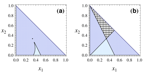
Figure 1: (Color online.) The structure of (12) on the simplex (1) [$0<x_{1}$, $0<x_{2}$, $0<x_{1}+x_{2}<1$] containing globally stable Nash equilibrium (37) (bold dot) for $n=3$ and $\vartheta=1$; see (44). Fig. 1(a): $b_{1}=b_{2}=b_{3}=0.3$. Fig. 1(b): $b_{1}=b_{2}=b_{3}=0.99$. The Le Chatelier principle supporting domain is shaded normally (blue). Light (blue) shaded domains support only the weak principle, where both strongest and weakest components of a perturbation grow. Meshed domains also support only the weak principle, but now both strongest and weakest components of a perturbation decrease. Such domains are absent for the situation presented on Fig. 1(a). The Nash equilibrium on Fig. 1(b) is not evolutionary stable, but still globally stable.

V.3 Mutualistic replicators

They are defined by condition $a_{ik}\geq 0=a_{kk}$. An internal Nash equilibrium need not exist for mutualistic replicators, but if exists, then (at least for $n=3$) it is globally stable; cf. (45) under $|b_{i}|\geq 1$ and Footnote 11.

Let us now show that for mutualistic replicators the weak principle holds, at least for $n=3$. Recall (31) and the discussion after it. If the weak principle were violated there would exist a $3\times 3$ matrix $a_{ik}+\widetilde{a}_{ik}$ whose non-diagonal (diagonal) elements are positive (zero), and whose determinant is zero (since it supports two internal [linearly independent] Nash equilibria). It is clear that such a matrix does not exist .

For the case (44) the mutualism (16) amounts to $|b_{i}|\leq\vartheta=1$. For $n=3$ the criteria of evolutionary stability reduce from (23) to

$$a_{13}^{[s]}\geq 0,\qquad 4a_{13}^{[s]}a_{23}^{[s]}\geq(a_{13}^{[s]}+a_{23}^{[s]}-a_{12}^{[s]})^{2}.$$ (46)

To illustrate various stability notions, let us assume that $\vartheta=1>b_{i}=b>0$. Now (45) implies that the Nash rest-point (37) is asymptotically stable. The evolutionary stability (46) is more restrictive, since it demands $b<\sqrt{3}/2$. The validity of the Le Chatelier principle for all local perturbations is even more restrictive, since it demands $b<1/3$; see (33) and Fig. 1. Recall that the weak principle always holds for mutualistic replicators. Hence the weak principle is more general than the evolutionary stability, and the latter does not imply the local validity of the principle.

Note that the weak Le Chatelier principle has the following two scenarios of validity: i) perturbations leading to growth, because both the weakest and the strongest component of the perturbation increase; ii) perturbations leading to decay, since now both the weakest and the strongest component decrease. Other types of perturbations for $n=3$ will either violate the weak principle or satisfy the proper principle. It should be clear that during the second scenario the system in a sense destablizes, because smaller sizes of groups means larger extinction risks. It is seen from Figs. 1 and 3 that generally both scenarios for the weak Le Chatelier principle are present. However, we observed that whenever for mutualistic replicators the principle holds for all local perturbations, the domains that support only the weak principle are exclusively of the first type: they suppport the growth of population and not its decay; see Fig. 1(a). This observation indicates that the local condition (33) does a play a certain global role as well.

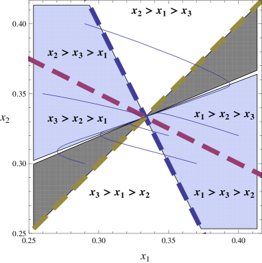
Figure 2: (Color online.) The local structure of (12) around asymptotically stable Nash equilibrium (37) under conditions (47). The parameters in (44) are: $\vartheta=1,\,b_{1}=2,\,b_{2}=1.2,\,b_{3}=2$. The Nash equilibrium (37) is asymptotically stable (with real eigenvalues of the linearized matrix $V_{ik}[p]$) but not globally stable, another asymptotically stable Nash equilibrium is $x_{1}=x_{2}=0$. The Le Chatelier principle supporting domain is shaded normally (blue). The domain where the weak principle is violated is shaded dark gray. Domains supporting only the weak principle are left blank. Three thick dashed lines are $x_{2}=x_{1}$, $x_{2}=1-2x_{1}$ and $x_{2}=(1-x_{1})/2$; as indicated, they bound regions with six different types of ordering. Ordinary lines denote typical trajectories of (12) moving towards (37) located at the crossing of three thick dashed lines.

V.4 Asymptotically, but not globally stable rest-point

For $n=3$ there are two possibilities for the replicator dynamics with an asymptotically stable, interior (and generic!) Nash equilibrium ${\bf p}>0$ zeeman . (i) it is globally stable: for all solutions with ${\bf x}(0)>0$ it holds ${\bf x}(t\to\infty)\to{\bf p}$. (ii) One of the vertices [vertex is a probability vector whose one component is $1$] is also asymptotically stable. This is the only vertex that is stable with respect to the boundary directions, and no other stable rest-points exist besides this vertex and ${\bf p}$. The vertex is also evolutionary stable, and thus the interior rest-point is not evolutionary stable; otherwise it had to be a unique Nash equilibrium hofbauer . We now turn to discussing the case (ii).

Let replicators 1 and 2 be mutualistic, but 1 gains more than 2 from this mutualism: $a_{12}>a_{21}>0$. Replicator 3 predates on 1 ($a_{13}<0$, $a_{31}>0$), but competes with 2: $a_{23},a_{32}<0$ (in a sense 2 saves 1 from 3). Hence the vertex $x_{3}=1$ is asymptotically stable; see (12). There can be also an internal asymptotically stable state if (paradoxically) 3 competes and predates strongly enough. Within parametrization (44) all the above conditions are satisfied for

$$\vartheta=1,~{}~{}~{}~{}b_{1}>b_{2}>1,~{}~{}~{}~{}b_{3}>\frac{b_{1}b_{2}-1}{b_{1}-b_{2}}>b_{2}>1,$$ (47)

where $b_{3}>\frac{b_{1}b_{2}-1}{b_{1}-b_{2}}$ comes from the asymptotic stability of the internal rest-point (37); see (45). Eq. (47) describes a generic situation with two asymptotically stable rest-points. Their attraction basins are detached by a separatrix that joins two rest points: $x_{1}=1$ and $(x_{1}=0,x_{2}=\frac{2b_{2}-2}{b_{2}+b_{3}-2})$.

The internal rest-point (37) is asymptotically stabilized by the assumed mutualism between 1 and 2. However, with respect to the Le Chatelier principle this rest-point is fragile: there are local perturbations that violate the weak principle ; see Fig. 2.

There are three types of perturbations for this situation: (1) supporting the Le Chatelier principle; (2) supporting the weak Le Chatelier principle only; (3) violating the weak Le Chatelier principle, i.e., transiently amplifying perturbation. Domains of the type (1) can be divided further into subdomains (1.1), where the trajectory remains confined to that domain for all times, i.e., (9) holds for all $\epsilon>0$, and subdomains (1.2), where the short-time response follows the Le Chatelier principle, but for intermediate times the trajectory leaves the domain. For the case shown in Fig. 2 all the trajectories end up in subdomains of the type (1.1). Circulation of trajectories around the Nash equilibrium is excluded, since the eigenvalues (45) are real.

V.5 Rock-scissors-paper [RSP] game

Cyclically dominant species are observed in nature and have certain unexpected features nz ; schuster . The cyclic dominance was proposed to be one of the basic mechanisms for maintaining diversity; see nz ; schuster and refs. therein. Their simplest model is the RSP game, where [recall that $a_{kk}=0$]:

$$a_{12},~{}~{}-a_{21},~{}~{}-a_{13},~{}~{}a_{31},~{}~{}a_{23},~{}~{}-a_{32}$$ (48)

are all positive meaning cyclic dominance; see (16–17).

The negativity of $a_{21},\,a_{13},\,a_{32}$ implies that for RSP the Le Chatelier principle cannot be satisfied for all local perturbations; see (33). For the case (44) the RSP conditions (48) amount to $b_{1}>\vartheta>0$, $b_{3}>\vartheta>0$ and $b_{2}<-\vartheta<0$. As the right Fig. 3 shows, provided that $|b_{i}|$’s are sufficiently different from each other, even the weak Le Chatelier principle can be violated in the vicinity of the globally stable Nash equilibrium (37). Thus cyclically dominating species can amplify small perturbations. The left part of Fig. 3 displays a scenario, where the principle is valid for four particular domains, while the weak principle holds everywhere. The situation with the zero sum game $a_{ik}=-a_{ki}$ is very similar to the left Fig. 3. Here the internal rest point ${\bf p}$ is only neutrally [not asymptotically] stable, i.e. ${\bf x}(t)$ does not converge to ${\bf p}$. However, the time-average converges to ${\bf p}$: $\int_{0}^{T}\frac{{\rm d}t}{T}\,{\bf x}(t)\to{\bf p}$ for $T\to\infty$ hofbauer . Although the notion of asymptotic stability does not apply, the Le Chatelier principle stays well-defined. We see an interplay between various notions of stability: RSP-replicators can violate the weak principle around an asymptotically stable rest-point [see the right Fig. 3], but neutrally stable zero-sum replicators satisfy the weak principle.

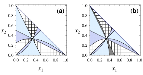
Figure 3: (Color online.) The structure of (12) on the simplex (1) with globally stable Nash equilibrium (37) (bold dot) for $n=3$ and $\vartheta=0.5$; see (44). Fig. 3(a): $b_{1}=1,\,b_{2}=-1,\,b_{3}=2$. Fig. 3(b): $b_{1}=1,\,b_{2}=-1,\,b_{3}=3$. The Le Chatelier principle supporting domain is shaded normally (blue). Light (blue) shaded domains support only the weak principle, where both strongest and weakest components of a perturbation grow. Meshed domains also support only the weak principle, but now both strongest and weakest components of a perturbation decrease. Regions violating the weak principle are shaded dark.

V.6 Summary

We now briefly summarize results obtained for three replicators for perturbations over an asymptotically stable, interior (and unique) Nash equilibrium.

• The Nash equilibrium is always in (or at the boundary of) the domain, where the Le Chatelier principle holds.

• The principle holds locally (i.e., for sufficiently weak perturbations) under condition (33) that implies mutualism.

• Whenever the principle holds locally, all other perturbations do not destabilize the system.

• Violations of the principle (or of its weak form) can show up already for arbitrary weak perturbations.

• The weak principle holds for an evolutionary stable Nash equilibrium. Even for such an equilibrium, the principle can be violated locally.

• The weak principle (and for certain perturbations the full principle) does hold for zer-sum replicators, whose Nash equilibrium is only neutrally stable.

VI Conclusion

In this paper we applied the Le Chatelier principle to replicator dynamics of Evolutionary Game Theory (EGT) aiming to understand how stability features of a Nash equilibrium resemble those of the thermodynamic equilibrium. Analogies between these two type of equilibria were noted at several instances bertin ; polish ; e.g., they both satisfy the notion of detailed balance (20).

The Le Chatelier principle states that a perturbation of an equilibrium state starts to diminish already on short times, in contrast to asymptotic stability, where perturbations are supposed to decay sooner or later. The Le Chatelier principle had several predecessors in natural philosophy phi and is widely known beyond its original application domain of quasi-equilibrium thermodynamics edu ; econo ; nature ; jorge ; gorshkov . However, its quantitative formulations is not widely known . Hence our first step was to reformulate the Le Chatelier principle for a non-linear master equation—a common framework for statistical physics and population dynamics—and relate it to the majorization concept. We were led to distinguish between the proper Le Chatelier principle (perturbation induces negative feedback) and its weak vesion (perturbation does not induce strong positive feedback).

Our results led to refining the notion of Nash equilibrium and evolutionary stability. The first result is that the validity of the Le Chatelier principle relates to mutualism. Other notions of stability (e.g., asymptotic stability) do not allow to indicate in which sense the mutualism can be more stable than other forms of interactions that also lead to an asymptotically stable [or even globally stable] interior rest-point . This conclusion points at a stability-based mechanism for explaining the emergence and maintenance of mutualistic interactions.

More generally, we noted that the viewpoint of the Le Chatelier principle allows to uncover rich scenarios of behaviour for a stable Nash equilibrium under perturbations. There are always perturbation domains, where the Le Chatelier principle is satisfied, but there are also perturbation domains, where only the weak principle holds. Moreover, certain non-mutualistic [e.g., cyclically competing] replicators with a single globally stable Nash equilibrium are capable of violating even the weak Le Chatelier principle, i.e., they are endowed with a strong form of positive feedback (weaker forms of positive feedback are possible already when only the weak principle holds). This is impossible for perturbations over a thermodynamic equilibrium, since there it would mean a negative entropy production.

The existence of positive feedback mechanisms is recognized in ecology at several instances. It is argued that younger [on the evolution scale] natural ecosystems have more positive feedback mechanisms than older ones, where negative feedback dominates svi . In macroevolution dynamics positive feedback is essential for the punctuated equilibrium: most species persist for ages without showing any significant morphological change [equilibrium], but they do display relatively sudden changes via a positive-feedback response after specific perturbations punctuated_equilibrium . Hence before the punctuation starts, the equilibrium state should be stable, but it cannot be ”equally stable” with respect to all possible perturbations. Clearly, this combination of various forms of stability (or rather various forms of feedback) can be quantified via the Le Chatelier principle.

We focussed on perturbations over an asymptotically stable (interior) Nash equilibrium. The Le Chatelier principle applies to replicators satisfying a weaker form of stability: permanence (or Lagrange stability) that rules out the extinction of any replicator that was present in the population initially svi ; hofbauer . Some important classes of replicators—e.g., those playing an asymmetric [two-population] or a zero-sum game—can be only permanent, e.g., for them a Nash equilibrium is not asymptotically stable (or even not stable, as for hypercyclic replicators) hofbauer ; sandholm . One problem with this type of stability is that a sequence of relatively weak perturbations may drive replicators towards the simplex boundary, where the extinction risks are high justus . The weak Le Chatelier principle will guarantee the absence of such a scenario, and its application to this situation is straightforward, because a permanent system of replicators (12) does have a unique (but generally not stable) interior Nash equilibrium ${\bf p}>0$, with time-averaged state converging to ${\bf p}$: $\int_{0}^{T}\frac{{\rm d}t}{T}\,{\bf x}(t)\to{\bf p}$ for $T\to\infty$ hofbauer . An example of studying permanence via the weak Le Chatelier principle was given above for a zero-sum game.

Here we restricted ourselves with perturbations of the state, i.e., the probability vector ${\bf x}$. The Le Chatelier principle should also be studied for structural perturbation that do not act directly on the state ${\bf x}$, but influence the structure of the system making the transition probabilities $W_{i\not=k}[{\bf x},\lambda_{t}]$ time-dependent via a parameter $\lambda_{t}$; see ives for the relevance of such perturbations in ecology.

There is a long history of applying thermodynamic stability principles to bio-ecological systems; see trincher ; ulan ; critics ; chakra ; karo ; rubin_fokht . These studies are definitely thought-provoking, e.g., an observation by Trincher trincher that the qualitative statement of the Le Chatelier principle is to be violated in the processes of embryogenesis inspired the present work (cf. with the above discussion on the punctuated equilibrium).

However, the basic tool in almost all such applications is the notion of entropy production, whose features (e.g., positivity) are invoked for making predictions about the stability of a bio-ecological system. This approach lacks operationalism, because for the entropy production to be well defined one should assume that the considered bio-ecological system is literally thermodynamical, i.e., that concepts developed within physics (thermodynamic equilibrium, the notions of entropy, temperature, forces and fluxes) apply. Obviously, an open and non-equilibrium bio-ecological system produces entropy somewhere and somehow, but one needs specific conditions for applying concepts developed within physics; in particular, it has to be verified that the formally introduced entropy production indeed has a physical meaning. This is best examplified by the current literature, e.g. Refs. chakra ; karo ; rubin_fokht ; andrae that claim to apply the entropy production concept to the same population dynamic models, all employ different definitions of this concept (albeit some of these definitions become equivalent in the vicinity of the rest-point; see chakra ; rubin_fokht ; andrae ). In contrast, the presented application of Le Chatelier principle is based on the operational notion of perturbation decay. Hence, its application need not assume any would-be-valid thermodynamic reasoning.

Acknowledgement. This work has been supported by Volkswagenstiftung.

References

- (1) V.B.E. Thomsen, Le Chatelier s Principle in the Sciences, J. Chem. Ed. 77, 173 (2000).
- (2) E.F. Keller, Organisms, Machines, and Thunderstorms: A History of Self-Organization I, Hist. Stud. Nat. Sci. 38.1, 45 (2008).
- (3) L.D. Landau and E.M. Lifshitz, Statistical Physics, I (Pergamon Press Oxford, 1978).
- (4) R. Gilmore, Le Chatelier reciprocal relations and the mechanic analog, Am. J. Phys. 51, 733 (1983).
- (5) W. Suen, E. Silberberg, and P. Tseng, The LeChatelier principle: the long and the short of it, Economic Theory 16, 471 (2000).
- (6) D.J. Bellamy and P.H. Clarke, Application of the second law of thermodynamics and Le Chatelier’s principle to the developing ecosystem, Nature, 218, 1180 (1968).
- (7) S.E. Jorgensen and B.D. Fath, Application of thermodynamic principles in ecology, Ecological Complexity 1, 267 (2004).
- (8) V. G. Gorshkov, Physical and Biological Bases of Life Stability (Springer-Verlag, Berlin, 1994).
- (9) Yu.M. Svirezhev and D.O. Logofet, Stability of Biological Communities (Mir Publications, Moscow, 1983).
- (10) A.R. Ives and S.R. Carpenter, Stability and Diversity of Ecosystems, Science 317, 58 (2007).
- (11) V. I. Arnold, Ordinary Differential Equations (Springer-Verlag, New-York, 1991).
- (12) E. C. Zeeman, Population dynamics from game theory, in Global theory of dynamical systems, Lecture Notes in Mathematics, 819, 471 (Springer, NY, 1980).
- (13) J. Hofbauer and K. Sigmund, Evolutionary Games and Population Dynamics (Cambridge Univ. Press, 1998).
- (14) W. H. Sandholm, Population Games and Evolutionary Dynamics (MIT Press, 2010).
- (15) A.A. Gimelfarb, L.R. Ginsburg, R.A. Poluektov, Yu.A. Pykh and V.A. Ratner, Dynamic theory of biological populations (Nauka, Moscow, 1974). [in Russian]
- (16) Yu.M. Svirezhev and V.P. Passekov, Findamentals of Mathematical Genetics (Dordrecht, Kluwer, 1990).
- (17) A. E. Allahverdyan and G. Mahler, Employing feedback in adiabatic quantum dynamics, EPL 84, 40007 (2008).
- (18) A. Menon, K. Mehrotra, C.K. Mohan and S. Ranka, Replicators, Majorization and Genetic Algorithms, in Foundations of genetic algorithms 4, ed. by R. K. Belew and M. D. Vose (Morgan Kaufmann, San Francisco, CA, 1997).
- (19) B. S. Lieberman and N. Eldredge, Punctuated equilibria, Scholarpedia, 3(1), 3806 (2008).
- (20) S.R. de Groot, Thermodynamics of Irreversible Processes (North Holland, Amsterdam, 1952).
- (21) K.S. Trincher, Biology and information, elements of biological thermodynamics (Consultants Bureau, NY, 1965).
- (22) N. G. van Kampen, Stochastic Processes in Physics and Chemistry (North Holland, Amsterdam, 1992).
- (23) E. Ruch and A. Mead, The principle of increasing mixing character and some of its consequences, Theoret. Chim. Acta (Berl.) 41, 95 (1976).
- (24) E. Ruch, R. Schranner and T.H. Seligman, The mixing distance, J. Chem. Phys. 69, 386 (1978).
- (25) A.W. Marshall and I. Olkin, Inequalities: Theory of Majorization and its Applications (Academic Press, New York, 1979).
- (26) E. Ruch and B. Lesche, Information extent and information distance, J. Chem. Phys. 69, 393 (1978).
- (27) F. Schlögl, Mixing distance and stability of steady states in statistical nonlinear thermodynamics, Z. Physik B 25, 411 (1976).
- (28) P. M. Alberti and B. Crell, Nonlinear evolution equations and H theorems, J. Stat. Phys. 35, 131, (1984).
- (29) M. Michalski, Non-linear, mixing dynamical systems, Rep. Math. Phys. 24, 305 (1986).
- (30) A. N. Gorban, P. A. Gorban, and G. Judge, The markov ordering approach, Entropy 12, 1145 (2010).
- (31) N.G. Chetaev, The stability of motion (Pergamon Press, NY, 1961).
- (32) E. Jen, Stable or robust? What is the difference?, in Robust Design, ed. by E. Jen (Oxford University Press, Oxford, 2005). J. Justus, Ecological and Lyanupov Stability, Phil. Science 75, 421, (2008).
- (33) E. Mayr, The objects of selection, PNAS, 94, 2091 (1997).
- (34) T.D. Frank, Physica A 331, 391 (2004).
- (35) V. N. Kolokoltsov, Nonlinear Markov processes and kinetic equations (Cambridge University Press, Cambridge, 2010).
- (36) T.D. Frank, Physica A 382, 453 (2007).
- (37) J.L. McCauley, Physica A 382, 445 (2007).
- (38) R. Lemoy, E. Bertin and P. Jensen, Socio-economic utility and chemical potential, EPL 93, 38002 (2011).
- (39) J. Miekisz, Stochastic stability in spatial games, J. Stat. Phys. 117, 99 (2004).
- (40) M. Frean and E.R. Abraham, Rock- scissors -paper and the survival of the weakest, Proc. R. Soc. Lond. B 268, 1323 (2001).
- (41) G. Neumann and S. Schuster, Continuous model for the rock scissors paper game between bacteriocin producing bacteria, J. Math. Biol. 54, 815 (2007).
- (42) R. E. Ulanowicz and B. M. Hannon, Life and the Production of Entropy, Proc. Royal Soc. London B, 232, 181 (1987).
- (43) T. Wilhelm and R. Bruggemann, Goal functions for the development of natural systems, Ecological Modelling 132, 231 (2000).
- (44) K. Michaelian, Thermodynamic stability of ecosystems, J. Theor. Biol. 237, 323 (2005).
- (45) C.G. Chakrabarti and K. Ghosh, Non-equilibrium thermodynamics of ecosystems: Entropic analysis of stability and diversity, Ecological Modelling 220, 1950 (2009).
- (46) A. B. Rubin and A. S. Fokht, On the determination of entropy increase rate for systems far from thermodynamic equilibrium, Biophysics, 17, 96 (1972).
- (47) B. Andrae, J. Cremer, T. Reichenbach, and E. Frey, Entropy Production of Cyclic Population Dynamics, Phys. Rev. Lett. 104, 218102 (2010).