A Refined QSO Selection Method Using Diagnostics Tests:
663 QSO Candidates in the LMC

Abstract

We present 663 QSO candidates in the Large Magellanic Cloud (LMC) selected using multiple diagnostics. We started with a set of 2,566 QSO candidates selected using the methodology presented in our previous work based on time variability of the MACHO LMC lightcurves. We then obtained additional information for the candidates by crossmatching them with the Spitzer SAGE, the 2MASS, the Chandra, the XMM, and an LMC UBVI catalog. Using this information, we specified six diagnostic features based on mid-IR colors, photometric redshifts using SED template fitting, and X-ray luminosities in order to further discriminate high confidence QSO candidates in the absence of spectra information. We then trained a one-class SVM (Support Vector Machine) model using the diagnostics features of the confirmed 58 MACHO QSOs. We applied the trained model to the original candidates and finally selected 663 high confidence QSO candidates. Furthermore, we crossmatched these 663 QSO candidates with the newly confirmed 151 QSOs and 275 non-QSOs in the LMC fields. On the basis of the counterpart analysis, we found that the false positive rate is less than 1%.

1. Introduction

Active Galactic Nuclei (AGNs) are very energetic extragalactic objects that have been studied in many astronomical fields such as galaxy formation and evolution (e.g. Heckman et al. 2004; Bower et al. 2006; Trichas et al. 2009, 2010), large scale structure (e.g. Ross et al. 2009), dark matter substructure (e.g. Miranda & Macciò 2007), and black hole growth (e.g. Kollmeier et al. 2006).

It is known that QSOs show strong variability over wide range of wavelengths on a time scale from a few days to several years (Hook et al., 1994; Hawkins, 2002). It is widely believed that the variability is associated with accretion disk instability (Rees, 1984; Kawaguchi et al., 1998). Recently, interesting studies on QSO variability have been published (Kelly et al., 2009; MacLeod et al., 2010), which confirmed a correlation between the time scale of QSO variability and the physical parameters of QSOs such as black hole mass. Although these studies confirmed the correlation, different studies showed a discrepancy at the time scales of QSO variability (Kelly et al., 2009; Kozłowski et al., 2010; MacLeod et al., 2010). Possible reasons for the discrepancy are 1) poorly-sampled lightcurves and/or short observational periods, 2) false positives such as stellar contaminations in their QSO candidates, and 3) biased QSO samples in luminosity or black hole mass. Thus having a well-sampled set of QSO lightcurves with a long baseline and small number of false positives is critical for the comprehensive analysis of this correlation. Note that there are only a few hundreds well-sampled QSO lightcurves, and a large portion of them are around the LMC fields where the MACHO survey monitored for several years (e.g. see Geha et al. 2003; Kelly et al. 2009; Kozłowski et al. 2011).

The MACHO survey observed the sky around the LMC for 7.4 years with relatively regular sampling of a few days. The majority of the MACHO lightcurves have more than several hundred data points and therefore the MACHO lightcurves are suitable for the QSO variability studies. Nevertheless, there are only 59 confirmed MACHO QSOs in the 40 deg² areas around the LMC (Geha et al., 2003). The main reasons for the relatively small number of QSOs are 1) the crowdedness of the fields, which makes it difficult to select QSO candidates among the dense stellar sources and thus yields a high false positive rate (e.g. see Geha et al. 2003; Dobrzycki et al. 2005), and 2) the high cost of spectroscopic or X-ray observations, which are the best methods for confirming QSOs. Thus a novel QSO selection algorithm with a high efficiency and a low false positive rate is essential to make the best use of the expensive spectroscopic telescope time and increase the collection of QSOs.

In our previous work (Kim et al., 2011), we developed a QSO selection method using a supervised classification model trained on a set of variability features extracted from the MACHO lightcurves including a variety of variable stars, non-variable stars and QSOs. The trained model showed high efficiency of 80% and low false positive rate of 25%. Using this method, we first selected 2,566 QSO candidates from the lightcurve database. We then developed and employed a decision procedure on the basis of diagnostics using 1) mid-IR colors, 2) photometric redshifts, and 3) X-ray luminosities on these candidates in order to separate high confidence QSO candidates (hereinafter hc-QSOs). As a result, we chose in total 663 hc-QSOs out of 2,566. These 663 candidates are likely QSOs; if confirmed this will increase the previous collection of QSOs in the MACHO LMC database by a factor of $\sim$12. Note that most of the hc-QSO lightcurves are well-sampled for 7.4 years (i.e. several hundreds data points with relatively regular sampling). and are chosen in such a way to exclude any potential false positives. Therefore the lightcurve collection of hc-QSOs is a valuable set for QSO variability studies and can be used as a target set for spectroscopic observations.

In Section 2, we briefly introduce the MACHO database and the QSO selection algorithm that we developed to select the initial set of QSO candidates. We then present multiple diagnostics that we applied on the set of QSO candidates in Section 3. Section 4 presents a classification model trained on the diagnostics features in order to choose hc-QSOs. In Section 5, we crossmatch our candidates with newly discovered QSOs in the LMC fields. A summary is given in Section 6.

2. QSO Candidates in the MACHO LMC database

We first selected QSO candidates from the MACHO lightcurve database using the QSO selection method developed by Kim et al. (2011) (hereinafter, K-method). In this paper we used a 10% QSO probability product cut to select the QSO candidates rather than a 25% cut which Kim et al. (2011) used because we will employ other diagnostics (see Section 3) that are able to effectively remove false positives. Here probability product is the product of the probabilities derived independently from MACHO B and R band lightcurves using Support Vector Machine (Boser et al., 1992) and Platt’s probability estimation (Platt, 1999). By definition, QSO candidates with higher probabilities are more likely to be QSOs. With the probability cut of 10%, we found 2,566 QSO candidates.

3. Diagnostics of the QSO Candidates

In the following subsections, we will introduce the diagnostics performed and the consequent results.

3.1. Spitzer mid-IR Properties

It is known that mid-IR color selection is an efficient discriminator for AGNs and stars/galaxies resulting from the fact that the spectral energy distributions of these sources are substantially different from each other (Laurent et al., 2000; Lacy et al., 2004). Lacy et al. (2004) introduced a mid-IR color cut to separate AGNs using Spitzer SAGE (Surveying the Agents of a Galaxy’s Evolution; Meixner et al. 2006) catalog. Kozłowski & Kochanek (2009) employed a similar mid-IR color cut and selected about 5,000 AGN candidates from the Spitzer SAGE catalog.

We used these mid-IR color selections as the first diagnostic. We crossmatched our candidates with the Spitzer SAGE LMC catalog containing 6 million mid-IR objects in order to check whether our candidates are inside the mid-IR selection cuts. We searched for the nearest SAGE source from each candidate within an 1^′′ search radius. In order to minimize false crossmatchings, we defined a source as a counterpart only if there are no other Spitzer sources within a 3^′′ radius from the candidate.

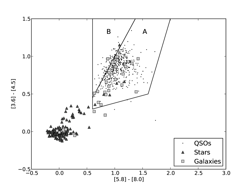
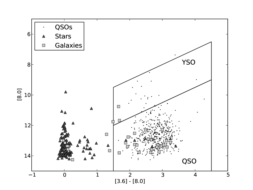
We found about 700 Spitzer counterparts shown in Figure 1 (dots). The sources inside region B could either be AGNs or stars, while the sources inside region A are likely AGNs. The YSO region is thought to be dominated by Young Stellar Objects (YSOs) while the QSO region is thought to be dominated by AGNs. Nevertheless, all the sources inside these four regions are potential QSOs. Almost all of the confirmed MACHO QSOs are inside these four regions as shown in Figure 1 (boxes). The candidates inside these regions are most likely broad emission line QSOs (i.e. Type I AGNs (Stern et al., 2005)). Among these counterparts, the sources inside both the QSO and the A regions are likely to be QSOs. We found that 469 QSO candidates are inside both QSO and A regions.

Figure 1.— Mid-IR color-color and color-magnitude diagrams of the Spitzer SAGE counterparts with our QSO candidates (dots). Each axis of the figure is either Spitzer magnitude or color. All sources inside the four regions A, B, QSO and YSO are potential QSOs (Kozłowski & Kochanek, 2009). There are 469 candidates inside the both QSO and A regions, which are the most promising QSO candidates. The confirmed MACHO QSOs are also inside these four regions (boxes).

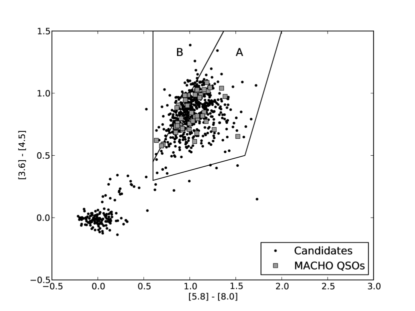
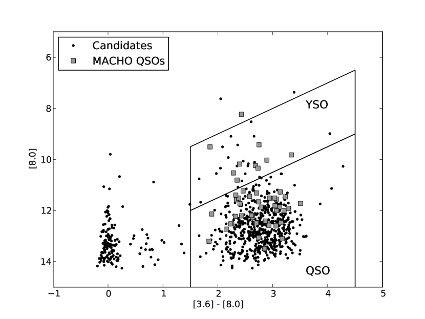
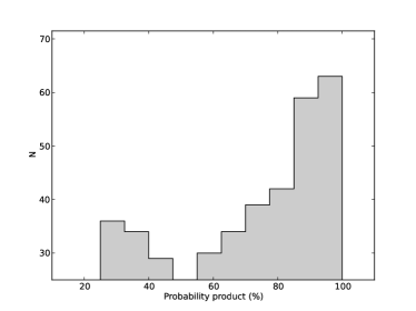
Figure 2 shows the estimated K-method QSO probability products of these 469 candidates. As the histogram shows, there are more QSO candidates at higher probability than lower probability, which implies that the mid-IR diagnostic is in line with the K-method. In addition, the histogram shows a bimodal distribution of the probabilities. We will address this bimodality in the following section.

Figure 2.— Histogram of K-method QSO probabilities of the SAGE counterparts inside both the QSO and the A (see Figure 1). There are more high probability candidates than low probability candidates, which indicates that the candidates inside the QSO and the A are likely to be QSOs. The histogram also shows a bimodal distribution as is addressed in Section 3.2.

3.2. Photometric Redshift Using Template Fitting

Figure 3.— Criterion (the solid line) to separate extragalatic sources (‘Galaxies and AGN’ in the figure) from stars (Eisenhardt et al., 2004; Rowan-Robinson et al., 2005) Using the criterion, 686 candidates were classified as extragalatic sources (above the line) and 1274 candidates were classified as stars (below the line).

We first crossmatched the 2,566 QSO candidates with the UBVI catalog for the LMC (Zaritsky et al., 2004) and the 2MASS catalog (Skrutskie et al., 2006) to extract UBVI and JHK magnitudes. We searched the nearest source from each of the candidates within a 3^′′ search radius. In the case of the UBVI catalog, we found in total 2,375 counterparts. Among them, 84% (93%) UBVI counterparts are within a 1^′′ (1.5^′′) distance from the candidates. In addition, only 0.3% (2% or 17%) of the candidates have another counterpart within an 1^′′ (1.5^′′ or 3^′′) distance from the candidates. Thus the portion of the false crossmatching is not significant. In the case of the 2MASS catalog, we found in total 846 counterparts. From those, 74% (83%) are within a 1^′′ (1.5^′′) distance from the candidates while 0% (0.1% or 0.5%) of the candidates have another counterpart within a 1^′′ (1.5^′′ or 3^′′) distance from the candidates. Again the portion of the false crossmatching is negligible.

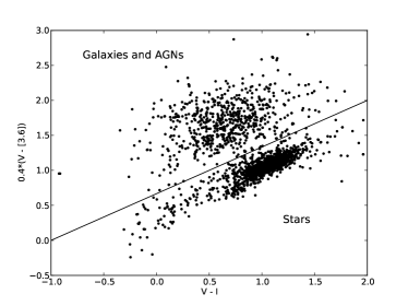
We then separated stars from ‘Galaxies and AGNs’ (i.e. extragalatic sources) using a criterion proposed by Eisenhardt et al. (2004) and Rowan-Robinson et al. (2005). Figure 3 shows the criterion (the solid line) we applied. There were 686 extragalatic sources (above the cut) and 1274 stars (below the cut). These 686 extragalatic sources were then fitted with galaxy templates in order to derive photometric redshifts (Rowan-Robinson et al., 2008). The templates contained three QSO, one starburst and 10 galaxy templates. For details about the photometric redshift estimations and the SED template fitting, see Rowan-Robinson et al. (2008).

Among the extragalatic sources, 602 were fitted with AGN templates (i.e. QSOs) while the remaining 84 were fitted with the galaxy templates (i.e. galaxies). These 602 candidates are likely QSOs. Figure 4 shows the photometric redshifts of these QSOs and galaxies. As the figure shows, the QSOs (the top panel) have relatively higher redshifts than the galaxies (the bottom panel). QSOs are much more luminous than galaxies and thus are detectable at higher redshifts than galaxies. In Figure 5, we show the comparison between the photometric redshifts and the spectroscopic redshifts of the confirmed MACHO QSOs (Geha et al., 2003). Out of the 58 confirmed MACHO QSOs, 40 are fitted with the photometric redshift code. The remaining 18 were not fitted due to the lack of data (i.e. UBVI magnitudes). Among these 40 confirmed MACHO QSOs, only one was best fitted with galaxy templates while the other 39 were fitted with AGN templates. The QSO best fitted with the galaxy templates is confirmed to be a QSO from the works done by Schmidtke et al. (1999); Geha et al. (2003). Out of the 40 QSOs, 28 (70%) are inside the $\pm$0.1 dex accuracy (the dashed line in the figure).

Figure 4.— Photometric redshifts of the 602 QSO candidates fitted with the AGN templates (the top panel) and the 84 QSO candidates fitted with the galaxy templates (the bottom panel) (Rowan-Robinson et al., 2008). The 602 QSO candidates show relatively larger redshifts than the 84 candidates.

Figure 5.— Comparison between the spectroscopic redshifts (Geha et al., 2003) and the photometric redshifts for the confirmed MACHO QSOs. Seventy percent of estimated redshifts are well-matched with the spectroscopic redshifts (see the dashed line corresponding to $\pm$0.1 dex accuracy). There is one MACHO QSO (triangle) that is fitted with the galaxy templates and 39 MACHO QSOs (squares) that are fitted with the AGN templates (Rowan-Robinson et al., 2008).

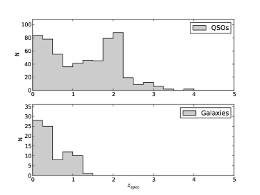
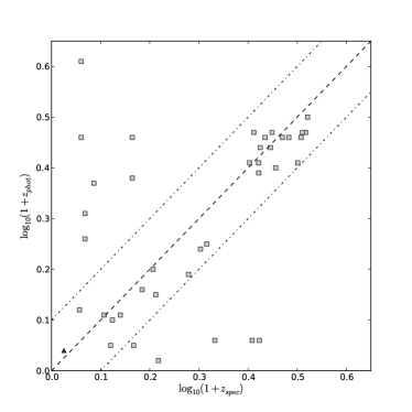
Figure 6 shows the K-method probability of QSOs, galaxies and stars discriminated during the photometric redshift estimation. As the figure shows, the majority of QSOs have higher probabilities than galaxies and stars, which implies that galaxies and stars have different and most likely weaker variability characteristics from/than QSOs. Note that the probabilities are from the K-method which mainly used variability features of lightcurves to select QSO candidates.

Figure 6.— left: Histogram of the estimated K-method QSO probabilities for 602 QSOs fitted with the AGN templates. The histogram shows a bimodal distribution similar to the histogram shown in Figure 2. The bimodality is correlated with different variability characteristics of the low and high probability QSO candidates. See the text and Figure 7 for details. right: Histogram of the estimated K-method QSO probability of 84 galaxies (the top panel) and 1274 stars (the bottom panel) separated using a approach proposed by Eisenhardt et al. (2004) and Rowan-Robinson et al. (2005). As the histogram clearly shows, they have relatively lower probabilities than QSOs.

Figure 7.— left side A, B, C and D: Histogram of one of the time series features, $\sigma/\bar{m}$ (Kim et al., 2011). Galaxies and stars show different distribution from both high and low probability QSOs while high and low probability QSOs do not show distinctive differences. right side A, B, C and D: Histogram of Stetson $K_{AC}$ (Kim et al., 2011). High probability QSOs show different distribution from low probability QSOs while galaxies and stars show almost identical distributions. As the histograms show, it seems that the bimodality in the left panel of Figure 6 is correlated with the different variability characteristics of each class. Further analysis of this bimodality is beyond the scope of this paper.

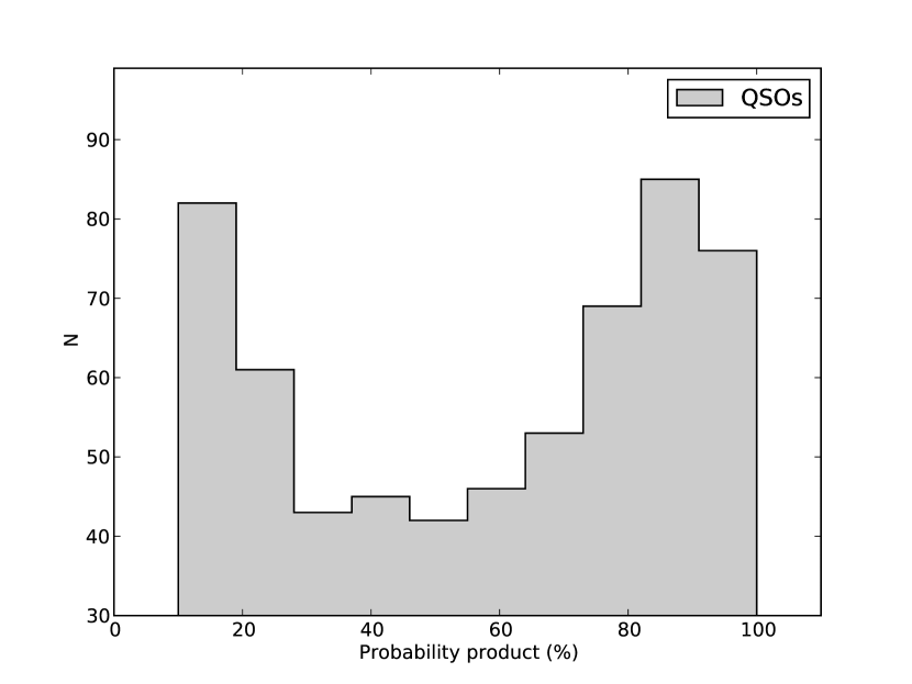
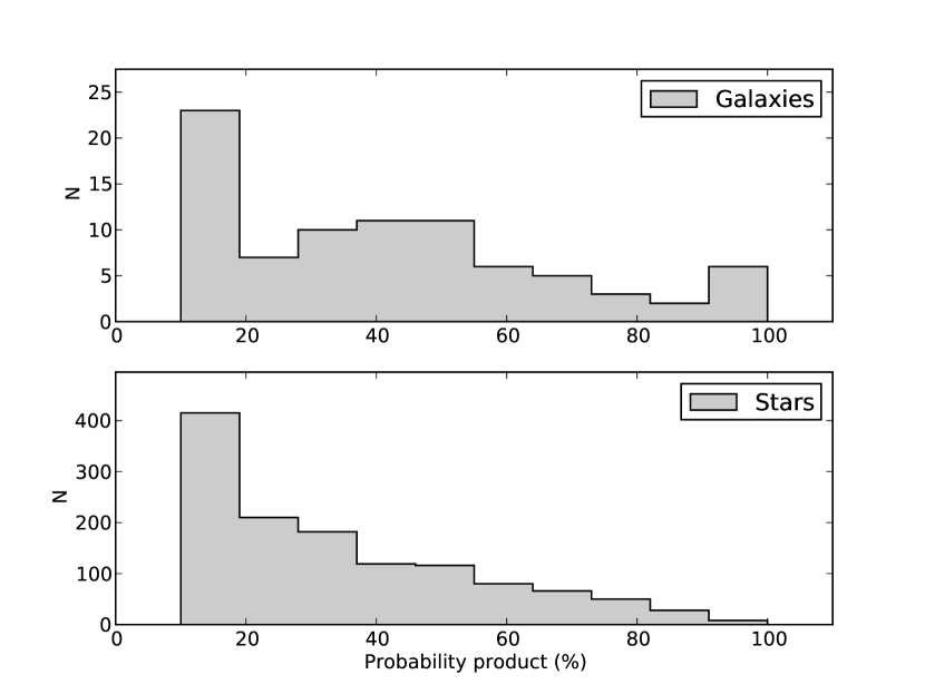
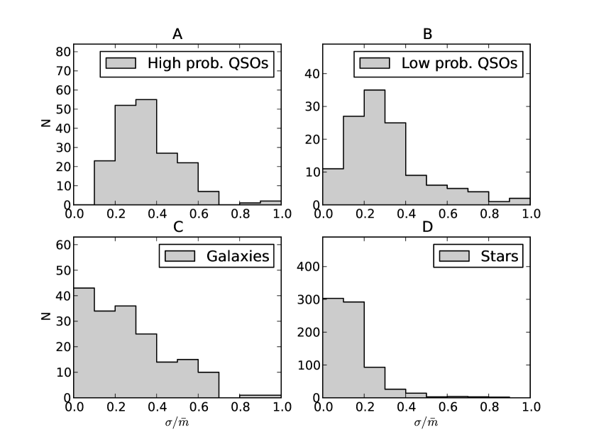
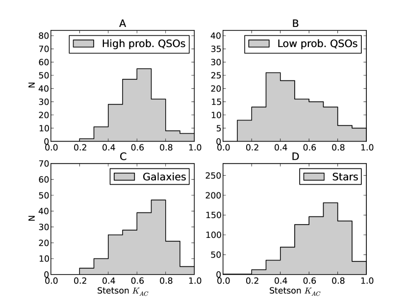
The left panel of Figure 6 also shows similar bimodality as seen in the Figure 2. In order to check if there exists 1) different variability characteristics between QSOs, galaxies and stars, and 2) different variability characteristics between the high and low probability QSO candidates, we show histograms of two variability features defined in Kim et al. (2011) in Figure 7. The left $2\times 2$ sub-panels (left side A, B, C and D) shows the histogram of $\sigma/\bar{m}$, where $\sigma$ is the standard deviation and $\bar{m}$ is the mean magnitude. In general $\sigma/\bar{m}$ is large when a lightcurve has strong variability. The x-axis is scaled to be between 0 and 1. To check if differences exist between high and low probability QSOs (A and B), we selected two subsets: one of high ($\geq$80%) and the other of low ($\leq$40%) probability QSOs. We included all galaxies (C) and stars (D) regardless of their probabilities. As the left panels show, galaxies and stars show different distributions from the distribution of QSOs that has a peak around $\sim$0.3. Nevertheless, high and low probability QSOs do not show different distribution. The right $2\times 2$ sub-panels (right side A, B, C and D) show a different time variability index, Stetson $K_{AC}$, which is the observation of the distribution of data points between the maximum and minimum values of the autocorrelation function of a lightcurve (Kim et al., 2011). As the panels show, high probability QSOs (A) show a peak around 0.6 while low probability QSOs (B) show a peak around 0.4. Galaxies (C) and stars (D) show peaks around 0.7. Thus it seems that the bimodality shown in the left panel of Figure 6 and the different distributions between QSOs, galaxies and stars in Figure 6 is correlated with the different variability characteristics of the lightcurves. Further analysis of this bimodality, requiring careful investigation of many variability characteristics and understanding of the selection biases is beyond the scope of this paper.

In addition, Figure 8 shows the mid-IR colors of QSOs, galaxies and stars. As the figure shows, almost all of the QSOs (dots) are inside the four regions while most of the stars (triangles) are outside the regions. Galaxies (squares) are either inside or outside the regions.

Figure 8.— Mid-IR color-color and color-magnitude diagrams of the QSOs, galaxies and stars classified using the photometric redshift code. See Section 3.2 for details. Each axis of the figure is either Spitzer magnitude or color. In the left panel, there are 502 QSOs (dots), 33 galaxies (squares) and 145 stars (triangles). In the right panel, there are 518 QSOs, 34 galaxies and 145 stars. As the figures show, almost all of the QSOs and galaxies are inside the regions (QSO, YSO, A and B), which indicates that all of them are potential QSOs. On the other hand, the majority of the stars are outside the regions.

3.3. X-ray Luminosity

Figure 9.— Scatter plot of the photometric redshifts (x-axis) and the estimated X-ray luminosity, ${\text{log}}{\,\text{L}}_{{\text{X}}}$, (y-axis). The dots are our QSO candidates and the x’s are the confirmed MACHO QSOs. left: XMM counterparts. right: Chandra counterparts. As the figures show, most of our candidates and MACHO QSOs have ${\text{log}}{\,\text{L}}_{{\text{X}}}>42$, which indicates they are likely QSOs.

Figure 10.— Mid-IR color-color and color-magnitude diagrams of the QSOs, galaxies and stars classified using the X-ray luminosity. See Section 3.3 for details. Each axis of the figure is either Spitzer magnitude or color. As the figures show, almost of the X-ray counterparts are within the QSO and the A region. The candidates inside the QSO and the A region are very likely QSOs (Kozłowski & Kochanek, 2009).

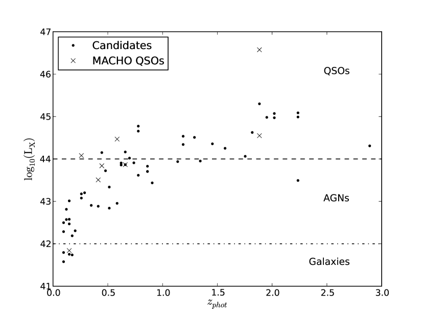
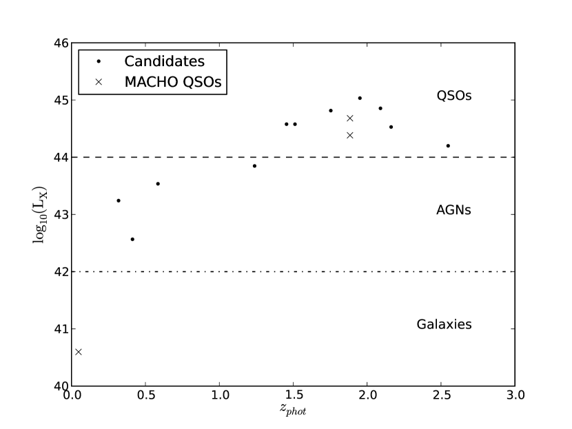
In order to estimate the X-ray luminosity, we crossmatched the 2,566 QSO candidates with two X-ray point source catalogs: the Chandra X-ray source catalog (Evans et al., 2010) and the XMM-Newton 2^nd Incremental Source catalog (Watson et al., 2009). We searched for the nearest source within a 5^′′ search radius from each candidate. The majority of the crossmatched counterparts were within a 3^′′ distance from the candidates and there were no additional counterparts within a 5^′′ distance from the candidates. We found 88 counterparts from either the XMM or Chandra catalogs.

Amongst the 88 counterparts, 64 were fitted with the SED templates mentioned in section 3.2 and therefore had estimated photometric redshifts. We used the photometric redshifts and X-ray fluxes from the catalogs to calculate the X-ray luminosity of each counterpart. Figure 9 shows the photometric redshifts (x-axis) and the estimated X-ray luminosity, ${\text{log}}{\,\text{L}}_{{\text{X}}}$ (y-axis). In the left panel, we show the 61 XMM counterparts including eight confirmed MACHO QSOs. The right panel shows 14 Chandra counterparts including three confirmed MACHO QSOs. Almost all of the candidates (60) have higher ${\text{log}}{\,\text{L}}_{{\text{X}}}$ than 42. In addition, six confirmed MACHO QSOs and 26 candidates show ${\text{log}}{\,\text{L}}_{{\text{X}}}$ higher than 44. The candidates showing higher ${\text{log}}{\,\text{L}}_{{\text{X}}}$ than 44 (42) are likely to be QSOs (AGNs) (Elvis et al., 1994; Persic et al., 2004). The remaining candidates that show lower ${\text{log}}{\,\text{L}}_{{\text{X}}}$ than 42 are likely to be galaxies.

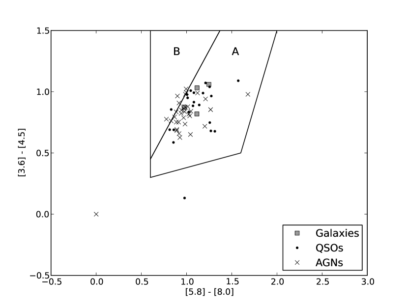
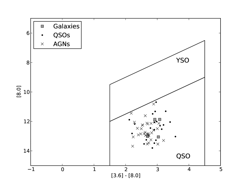
We show the mid-IR colors of these X-ray counterparts in Figure 10. The classification of QSOs (dots), AGNs (x’s) and galaxies (squares) are based on the X-ray luminosity of the counterparts.

4. High Confidence QSO Candidate Selection Using Support Vector Machines

4.1. Support Vector Machine

SVM (Support Vector Machine, Boser et al. 1992) is a supervised machine learning algorithm that trains a two-class classification model using samples of two known classes (i.e. training set). SVM is currently one of the best classification methods in machine learning. The classifier of a SVM defines a linear hyperplane that separates two classes in a training data. To select a unique hyperplane among the set of possible hyperplanes that separate the data, SVM chooses the hyperplane which maximizes the margin between the two classes, and is therefore often called the maximum margin separator. SVM is also able to separate non-linearly separable classes by using a kernel function (e.g. a polynomial kernel or a radial basis kernel) transforming non-linear feature spaces into linear feature spaces. The hypothesis of SVM has the form:

$$Class(z)=\mbox{sign}(\sum_{i}\alpha_{i}y_{i}K(z,x_{i})-b)$$ (1)

where $i$ are the indices for training set examples, $x_{i}$ are the examples, $y_{i}$ are the labels, $z$ is the example that we are predicting the label for, $K(z,x_{i})$ is a kernel function, and $b$ is a threshold. The $\alpha_{i}$ are the parameters learned by the training procedure. Despite the mapping to a potentially high dimensional space using a kernel function, the maximum margin criterion leads to automatic capacity control and thus avoids overfitting.

Compared to neural networks, SVMs provide a flexible classification model, avoids the problems of local minima, and reduces the need for parameter tuning. For an overview, discussion and practical details, see Cristianini & Shawe-Taylor (2000); Bennett & Campbell (2000); Hsu et al. (2003); Kim et al. (2011) and references therein. Because standard SVM can only solve a two-class problem, Schölkopf et al. (2001) proposed a method to solve one-class classification problems using SVM. In brief, they define the origin as the second class and separate the one class from the origin using SVM. For details about the method, see Schölkopf et al. (2001); Manevitz & Yousef (2002).

4.2. Training a one-class SVM to Select High Confidence QSO Candidates

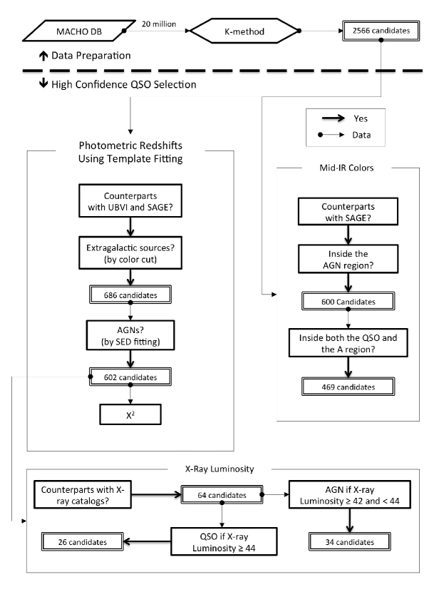
We employed the one-class SVM classification method to select high confidence QSO candidates because we do not have negative examples (i.e. non-QSO training set). We used a linear kernel rather than a polynomial kernel or a radial basis kernel because we empirically found that using other kernels did not improve classification results. To train a model, we first defined the diagnostics results as feature vectors. Table 1 summarizes the feature vectors. When we could not determine a feature value due to the nonexistence of counterpart with either the Spitzer SAGE, UBVI and X-ray catalogs, we assigned zero to the corresponding feature. Figure 11 outlines the calculation of the diagnostics and the number of candidates for which the diagnostics are available. As mentioned above, we started with the 2,566 QSO candidates selected using the K-method (‘Data Preparation’ panel in the figure). The diagnostics applied to these candidates are shown in the ‘High Confidence QSO Selection’ panel. We also show the number of QSO candidates after the diagnostics (double-lined rectangles).

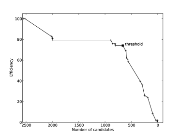
We trained a one-class SVM model using these features. We then tuned the model by adjusting the threshold, $b$, in order to: 1) obtain the highest efficiency based on the confirmed 58 MACHO QSOs, and 2) minimize the number of selected QSO candidates, which reduces the number of false positives as well. Figure 12 shows the efficiency and the number of candidates as a function of $b$. The black square shows the threshold we finally adopted. Using the determined threshold, the trained model showed 74% efficiency. We applied the tuned model to the 2,566 QSO candidates and selected 663 QSO candidates (i.e. hc-QSOs).

Table 2 shows a few important parameters for some of the QSO candidates. The entire parameters of the 2,566 QSO candidates are published in the electronic edition of this manuscript. We also provide catalogs and lightcurves of all the candidates at http://timemachine.iic.harvard.edu/coati/QSOs.

Table 1Feature Vectors

mid-IR	extragalactic sources/stars	SED fitting	$\chi^{2}$	Chandra	XMM
no CP : 0	no CP : 0	no CP : 0	no CP : 0	no CP : 0	no CP : 0
inside any of the four regions : 1	stars : 1	galaxies : 1	$\chi^{2}$ value	galaxies : 1	galaxies : 1
inside both the QSO and A region : 2	extragalactic sources : 2	AGNs : 2		AGNs : 2	AGNs : 2
				QSOs : 3	QSOs : 3

Figure 11.— Illustration of the processes that we used to select hc-QSOs. The rectangles with bold borderlines are the diagnostics. At most of the diagnostics, we determined if the candidates are likely to be QSOs (solid line arrows). The thin arrows show the data flow. The double-lined rectangles show the number of candidates.

Figure 12.— Efficiency versus number of selected QSO candidates as a function of the SVM threshold, $b$. The black square shows the final threshold we adopted.

Table 2Several Important Parameters of the QSO candidates

MACHO ID	RA	Dec	V	hc-QSO
	(in degree)	(in degree)	(mag)
11.8747.1083	83.52708	-70.62689	18.98	1
11.8753.346	83.66207	-70.20544	18.72
11.8984.29	83.89623	-70.89459	18.16
11.8989.258	84.04636	-70.61672	18.67
11.8994.1323	83.91927	-70.25463	19.27	1
11.9349.1074	84.53299	-70.81329	20.26	1
11.9353.1217	84.52798	-70.50399	19.52
12.10679.528	86.51372	-70.85550	18.99
13.5834.232	79.19451	-71.16704	19.57
13.6446.758	80.00723	-70.74329	20.32
13.6448.3756	80.03121	-70.59326	19.04
13.6560.555	80.25070	-71.21474	19.68

Note: This table is published in its entirety in the electronic edition of this manuscript. A portion is shown here for guidance regarding its form and content.

5. Crossmatching with Newly Discovered QSOs by KozŁowski (2011)

Recently, Kozłowski et al. (2011) selected QSO candidates using mid-IR colors, X-ray emission and/or optical variability in the OGLE lightcurve database (Udalski et al., 2008). For the variability selection, they used the DRW (a Damped Random Walk) model of lightcurves (Kelly et al., 2009; Kozłowski et al., 2010) and then applied several cuts including magnitude, model fitting accuracy, slope of a structure function, amplitude and time scale of lightcurve variations. They then visually examined all the lightcurves of the candidates and removed about 96% of lightcurves ($\sim$23,000) from the final list. Most of false positives were the ‘ghost’ variable objects caused by photometric defects. They finally observed 845 QSO candidates using AAT/AAOmega and confirmed 169 QSOs including 25 previously known QSOs (i.e. 144 newly discovered QSOs) in the four $\sim$3 deg² field near the LMC center. They also provided the list of remaining 676 objects. Among these 676 objects, they confirmed that 275 are non-QSOs, including young stellar objects (YSOs), red stars, blue stars, Be stars and planetary nebulae.

To estimate the efficiency and the false positive rate of our selection method, we first crossmatched the 151 discovered QSOs and 275 confirmed non-QSOs (i.e. false positives) with the entire MACHO LMC lightcurve database. We searched the nearest MACHO LMC source within a 3^′′ search radius. Out of 151 QSOs and 275 non-QSOs, 64 and 122 were crossmatched with the MACHO sources. Note that, only 46 out of 64 were selected using variability characteristics in the OGLE-III lightcurves (Kozłowski et al., 2011).

Among these 46 QSOs, 20 are in the hc-QSO list (hereinafter, c-QSOs) and 26 are not in the hc-QSO list (hereinafter, cn-QSOs), which gives us 43% efficiency. It is worth mentioning that the yield of QSO candidates from Kozłowski et al. (2011) selected using only variability based on the DRW model was 7%.

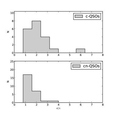
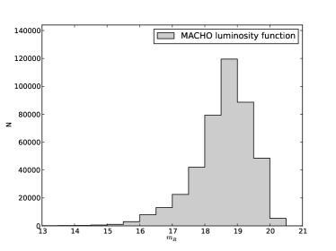
Despite of the fact that these 46 QSOs were determined to be variable objects based on the optical OGLE-III lightcuves, some of them do not show strong variability in the MACHO lightcurves because of 1) the difference of the limiting magnitudes of the two survey, and 2) the photometric uncertainty of the MACHO lightcurves. For instance, we found that 11 of cn-QSOs are fainter than 19 MACHO R magnitude ($m_{R}$) while only two of c-QSOs are fainter than 19 $m_{R}$, which is around a limiting magnitude of MACHO survey (Figure 15). Thus it is likely that the K-method using variability was not able to detect some of the QSOs due to the large photometric uncertainty and thus weak variability. Figure 13 shows the histogram of the ratio between the average photometric uncertainty and standard deviation (i.e. amplitude), $\sigma/\epsilon$, of the lightcurves of c-QSOs and cn-QSOs. Small $\sigma/\epsilon$ means that the photometric uncertainty is relatively larger than the amplitude of the lightcurve, which implies that it is rather hard to detect its variability. As the figure shows, c-QSOs have relatively larger $\sigma/\epsilon$ than cn-QSOs, which means c-QSOs are more detectable than cn-QSOs using their variability. $\sigma$ is one of the time variability features that the K-method used.

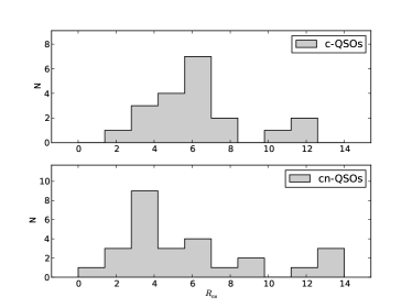
In Figure 14, we show an alternative way of seeing variability characteristic of a lightcurve by borrowing one example of the time series features, $R_{cs}$ (Ellaway, 1978), used in the K-method. $R_{cs}$, the range of a cumulative sum, is typically large for the variables showing non-periodic and strong variability, and is small for periodic variables or non-variables. As the figure shows, the histogram of c-QSOs (the top panel) has a peak around 6 while the histograms of cn-QSOs shows a peak around 3 (the bottom panel).

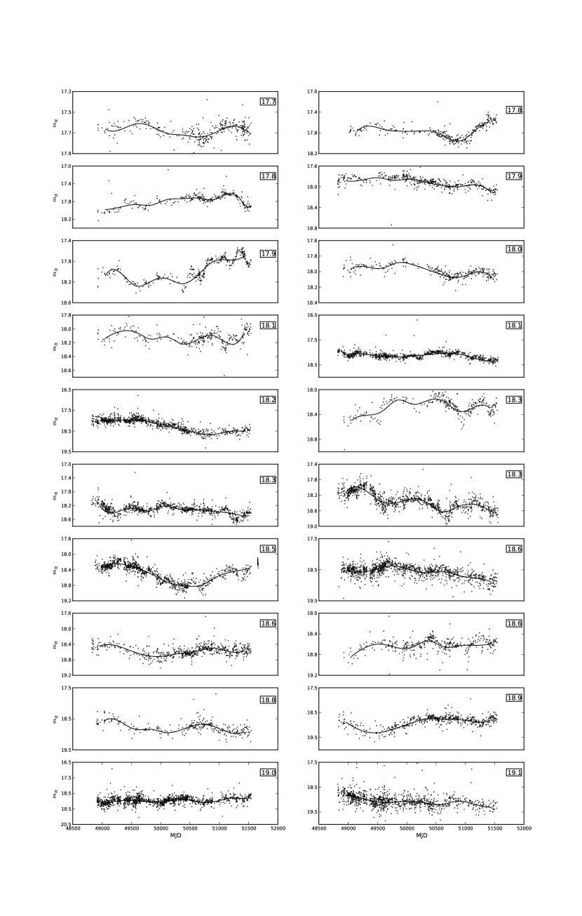
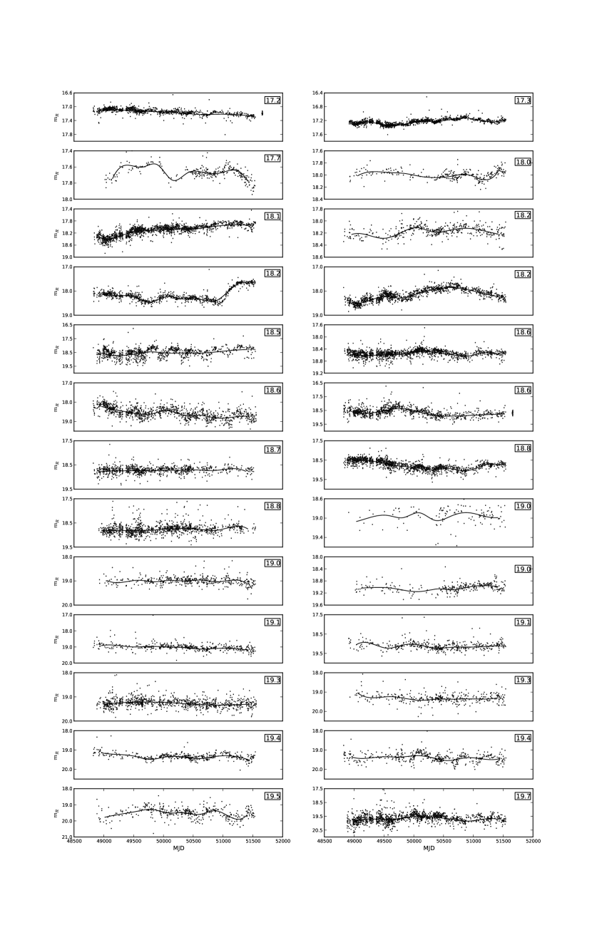
In addition, we show the MACHO lightcurves of the 20 c-QSOs and 26 cn-QSOs in Figure 16 and Figure 17. As Figure 16 shows, most of the c-QSOs show strong variability. On the other hand, Figure 17 shows that most of the cn-QSOs fainter than 19 $m_{R}$ show relatively weaker variability than the variability of c-QSOs. Only cn-QSOs brighter than 19 $m_{R}$ shows strong variability comparable to that of c-QSOs.

According to Figure 13, 14, 16 and 17, it seems that the main reason for the non-detection of QSOs is the relatively weaker variability. Thus if we ignore some of the QSOs showing weak variability, our efficiency would be higher than 43%. For instance, if we ignore the 11 cn-QSOs fainter than 19 $m_{R}$, our efficiency increases to 57%.

Figure 13.— Histogram of the ratio between the photometric uncertainty and amplitude, $\sigma/\epsilon$, of c-QSOs (the top panel) and cn-QSOs (the bottom panel). See the text for details about c-QSOs and cn-QSOs. Small $\sigma/\epsilon$ means that the photometric uncertainty is too large to detect variability. c-QSOs show relatively larger $\sigma/\epsilon$ than cn-QSOs, which means that c-QSOs are more detectable than cn-QSOs using variability.

Figure 14.— Histogram of $R_{cs}$ of c-QSOs (the top label) and cn-QSOs (the bottom panel). c-QSOs and cn-QSOs show different distribution. See the text for details.

Figure 15.— Luminosity function of MACHO R magnitude from one MACHO field. The x-axis is MACHO R magnitude and the y-axis is the number of MACHO sources. As the figure shows, the limiting R magnitude is around 19 $\sim$ 19.5.

Figure 16.— MACHO B band lightcurves of c-QSOs. The x-axis is MJD and the y-axis is MACHO R magnitude ($m_{R}$). The solid lines are the smoothed spline lightcurves. The small boxes inside each panel show the average $m_{R}$. As the figure shows, almost all the lightcurves show strong variability regardless of their magnitudes.

Figure 17.— MACHO B band lightcurves of cn-QSOs. When compared to the lightcurves shown in Figure 16, these lightcurves show relatively weaker variability. Moreover, there are a lot more fainter lightcurves than the lightcurves in Figure 16.

In the case of the false positives, only two out of 122 confirmed non-QSOs are inside the hc-QSO list, which gives 0.3% false positive rate. The two false positives are YSOs. We examined the MACHO lightcurves of them and confirmed that they show strong variability. Note that Kozłowski et al. (2011) monitored 12 deg² fields around the LMC that are mostly inside the 40 deg² MACHO LMC fields. Given that our QSO candidates are uniformly distributed around the LMC, we would have about one third number of the hc-QSOs ($12/40$) inside the fields that Kozłowski et al. (2011) monitored. In such case, the false positive rate is about 1%. However the true false positive rate would be higher than 1% because Kozłowski et al. (2011) did not monitor all the sources in the fields, which means some of our QSO candidates are not in their list. Nevertheless, these 122 non-QSOs were selected not only by variability but also by mid-IR colors and X-ray emission. Thus it seems that our method is successful to exclude any type of false positives, which is crucial for the selection of QSO candidates from massive astronomical databases such as Pan-STARRS (Kaiser, 2004) and LSST (Ivezic et al., 2008) due to: 1) the enormous amount of data, which thus could yield huge number of false positives, and 2) the high cost of spectroscopic observations for such deep and wide field surveys.

6. Summary

In this paper, we presented 663 high confidence QSO candidates, in the LMC fields. We first selected 2,566 QSO candidates based on the time variability of MACHO B and R band lightcurves in the MACHO LMC ligtcurve database using the method of Kim et al. (2011). We then applied multiple diagnostics such as mid-IR color, photometric redshift and X-ray luminosity to these QSO candidates. Using the diagnostics outputs, we trained a one-class SVM model to discriminate high confidence QSO candidates. We finally applied the trained model to the original candidates and selected 663 QSO candidates.

To estimate the yield and false positive rate of the final list, we crossmatched them with recently confirmed QSOs and non-QSOs in the LMC field (Kozłowski et al., 2011). As a result, we found that the yield is higher than $43\%$. It is worth mentioning that the yield of the QSO candidates selected using the ‘damped random work’ model (Kelly et al., 2009) is 7% (Kozłowski et al., 2011) . In the case of the false positive rate, we found that there are only a few confirmed non-QSOs in our list, which is less than 1% false positive rate. Thus this set could be used as a target set potential for spectroscopic survey to maximize the yield. This is important because the spectroscopic observations for relatively faint objects such as the QSO candidates in dense- and wide-field area around the LMC is extremely expensive. We are planning to use the confirmed QSOs and confirmed non-QSOs to improve our QSO selection method. This work will be separately published in the near future.

We will apply our method to the MACHO SMC/bulge database and the Pan-STARRS MDF (Medium Deep Field) time series database to further select QSO candidates and thus increase the collection of QSO lightcurves.

References

- Bennett & Campbell (2000) Bennett, K. P., & Campbell, C. 2000, SIGKDD Explorations, 2, 1
- Boser et al. (1992) Boser, B. E., Guyon, I. M., & Vapnik, V. N. 1992, in Proceedings of the fifth annual workshop on Computational learning theory, COLT ’92 (New York, NY, USA: ACM), 144–152
- Bower et al. (2006) Bower, R. G., Benson, A. J., Malbon, R., Helly, J. C., Frenk, C. S., Baugh, C. M., Cole, S., & Lacey, C. G. 2006, MNRAS, 370, 645
- Chang & Lin (2001) Chang, C. C., & Lin, C. J. 2001, LIBSVM : a library for support vector machines, http://www.csie.ntu.edu.tw/cjlin/libsvm
- Cristianini & Shawe-Taylor (2000) Cristianini, N., & Shawe-Taylor, J. 2000, An Introduction to Support Vector Machines (Cambridge: Cambridge Univ. Press)
- Dobrzycki et al. (2005) Dobrzycki, A., Eyer, L., Stanek, K. Z., & Macri, L. M. 2005, A&A, 442, 495
- Eisenhardt et al. (2004) Eisenhardt, P. R., Stern, D., Brodwin, M., Fazio, G. G., Rieke, G. H., Rieke, M. J., Werner, M. W., Wright, E. L., Allen, L. E., Arendt, R. G., Ashby, M. L. N., Barmby, P., Forrest, W. J., Hora, J. L., Huang, J., Huchra, J., Pahre, M. A., Pipher, J. L., Reach, W. T., Smith, H. A., Stauffer, J. R., Wang, Z., Willner, S. P., Brown, M. J. I., Dey, A., Jannuzi, B. T., & Tiede, G. P. 2004, ApJS, 154, 48
- Ellaway (1978) Ellaway, P. 1978, Electroencephalography and Clinical Neurophysiology, 45, 302
- Elvis et al. (1994) Elvis, M., Wilkes, B. J., McDowell, J. C., Green, R. F., Bechtold, J., Willner, S. P., Oey, M. S., Polomski, E., & Cutri, R. 1994, ApJS, 95, 1
- Evans et al. (2010) Evans, I. N., Primini, F. A., Glotfelty, K. J., Anderson, C. S., Bonaventura, N. R., Chen, J. C., Davis, J. E., Doe, S. M., Evans, J. D., Fabbiano, G., Galle, E. C., Gibbs, II, D. G., Grier, J. D., Hain, R. M., Hall, D. M., Harbo, P. N., (Helen He, X., Houck, J. C., Karovska, M., Kashyap, V. L., Lauer, J., McCollough, M. L., McDowell, J. C., Miller, J. B., Mitschang, A. W., Morgan, D. L., Mossman, A. E., Nichols, J. S., Nowak, M. A., Plummer, D. A., Refsdal, B. L., Rots, A. H., Siemiginowska, A., Sundheim, B. A., Tibbetts, M. S., Van Stone, D. W., Winkelman, S. L., & Zografou, P. 2010, ApJS, 189, 37
- Geha et al. (2003) Geha, M., Alcock, C., Allsman, R. A., Alves, D. R., Axelrod, T. S., Becker, A. C., Bennett, D. P., Cook, K. H., Drake, A. J., Freeman, K. C., Griest, K., Keller, S. C., Lehner, M. J., Marshall, S. L., Minniti, D., Nelson, C. A., Peterson, B. A., Popowski, P., Pratt, M. R., Quinn, P. J., Stubbs, C. W., Sutherland, W., Tomaney, A. B., Vandehei, T., & Welch, D. L. 2003, AJ, 125, 1
- Hawkins (2002) Hawkins, M. R. S. 2002, MNRAS, 329, 76
- Heckman et al. (2004) Heckman, T. M., Kauffmann, G., Brinchmann, J., Charlot, S., Tremonti, C., & White, S. D. M. 2004, ApJ, 613, 109
- Hook et al. (1994) Hook, I. M., McMahon, R. G., Boyle, B. J., & Irwin, M. J. 1994, MNRAS, 268, 305
- Hsu et al. (2003) Hsu, C.-W., Chang, C.-C., & Lin, C.-J. 2003, A practical guide to support vector classification, Tech. rep., Department of Computer Science, National Taiwan University
- Ivezic et al. (2008) Ivezic, Z., Tyson, J. A., Allsman, R., Andrew, J., Angel, R., & for the LSST Collaboration. 2008, ArXiv e-prints
- Kaiser (2004) Kaiser, N. 2004, in Society of Photo-Optical Instrumentation Engineers (SPIE) Conference Series, Vol. 5489, Society of Photo-Optical Instrumentation Engineers (SPIE) Conference Series, ed. J. M. Oschmann Jr., 11–22
- Kawaguchi et al. (1998) Kawaguchi, T., Mineshige, S., Umemura, M., & Turner, E. L. 1998, ApJ, 504, 671
- Kelly et al. (2009) Kelly, B. C., Bechtold, J., & Siemiginowska, A. 2009, ApJ, 698, 895
- Kim et al. (2011) Kim, D.-W., Protopapas, P., Byun, Y.-I., Alcock, C., Khardon, R., & Trichas, M. 2011, ApJ, 735, 68
- Kollmeier et al. (2006) Kollmeier, J. A., Onken, C. A., Kochanek, C. S., Gould, A., Weinberg, D. H., Dietrich, M., Cool, R., Dey, A., Eisenstein, D. J., Jannuzi, B. T., Le Floc’h, E., & Stern, D. 2006, ApJ, 648, 128
- Kozłowski & Kochanek (2009) Kozłowski, S., & Kochanek, C. S. 2009, ApJ, 701, 508
- Kozłowski et al. (2011) Kozłowski, S., Kochanek, C. S., Jacyszyn, A. M., Udalski, A., Szymanski, M. K., Poleski, R., Kubiak, M., Soszynski, I., Pietrzynski, G., Wyrzykowski, L., Ulaczyk, K., & Pietrukowicz, P. 2011, ArXiv e-prints:1106.3110
- Kozłowski et al. (2010) Kozłowski, S., Kochanek, C. S., Udalski, A., Wyrzykowski, Ł., Soszyński, I., Szymański, M. K., Kubiak, M., Pietrzyński, G., Szewczyk, O., Ulaczyk, K., Poleski, R., & The OGLE Collaboration. 2010, ApJ, 708, 927
- Lacy et al. (2004) Lacy, M., Storrie-Lombardi, L. J., Sajina, A., Appleton, P. N., Armus, L., Chapman, S. C., Choi, P. I., Fadda, D., Fang, F., Frayer, D. T., Heinrichsen, I., Helou, G., Im, M., Marleau, F. R., Masci, F., Shupe, D. L., Soifer, B. T., Surace, J., Teplitz, H. I., Wilson, G., & Yan, L. 2004, ApJS, 154, 166
- Laurent et al. (2000) Laurent, O., Mirabel, I. F., Charmandaris, V., Gallais, P., Madden, S. C., Sauvage, M., Vigroux, L., & Cesarsky, C. 2000, A&A, 359, 887
- MacLeod et al. (2010) MacLeod, C. L., Ivezić, Ž., Kochanek, C. S., Kozłowski, S., Kelly, B., Bullock, E., Kimball, A., Sesar, B., Westman, D., Brooks, K., Gibson, R., Becker, A. C., & de Vries, W. H. 2010, ApJ, 721, 1014
- Manevitz & Yousef (2002) Manevitz, L. M., & Yousef, M. 2002, J. Mach. Learn. Res., 2, 139
- Meixner et al. (2006) Meixner, M., Gordon, K. D., Indebetouw, R., Hora, J. L., Whitney, B., Blum, R., Reach, W., Bernard, J.-P., Meade, M., Babler, B., Engelbracht, C. W., For, B.-Q., Misselt, K., Vijh, U., Leitherer, C., Cohen, M., Churchwell, E. B., Boulanger, F., Frogel, J. A., Fukui, Y., Gallagher, J., Gorjian, V., Harris, J., Kelly, D., Kawamura, A., Kim, S., Latter, W. B., Madden, S., Markwick-Kemper, C., Mizuno, A., Mizuno, N., Mould, J., Nota, A., Oey, M. S., Olsen, K., Onishi, T., Paladini, R., Panagia, N., Perez-Gonzalez, P., Shibai, H., Sato, S., Smith, L., Staveley-Smith, L., Tielens, A. G. G. M., Ueta, T., van Dyk, S., Volk, K., Werner, M., & Zaritsky, D. 2006, AJ, 132, 2268
- Miranda & Macciò (2007) Miranda, M., & Macciò, A. V. 2007, MNRAS, 382, 1225
- Persic et al. (2004) Persic, M., Rephaeli, Y., Braito, V., Cappi, M., Della Ceca, R., Franceschini, A., & Gruber, D. E. 2004, A&A, 419, 849
- Platt (1999) Platt, J. C. 1999, in Advances in Large Margin Classifiers (MIT Press), 61–74
- Rees (1984) Rees, M. J. 1984, ARA&A, 22, 471
- Ross et al. (2009) Ross, N. P., Shen, Y., Strauss, M. A., Vanden Berk, D. E., Connolly, A. J., Richards, G. T., Schneider, D. P., Weinberg, D. H., Hall, P. B., Bahcall, N. A., & Brunner, R. J. 2009, ApJ, 697, 1634
- Rowan-Robinson et al. (2008) Rowan-Robinson, M., Babbedge, T., Oliver, S., Trichas, M., Berta, S., Lonsdale, C., Smith, G., Shupe, D., Surace, J., Arnouts, S., Ilbert, O., Le Févre, O., Afonso-Luis, A., Perez-Fournon, I., Hatziminaoglou, E., Polletta, M., Farrah, D., & Vaccari, M. 2008, MNRAS, 386, 697
- Rowan-Robinson et al. (2005) Rowan-Robinson, M., Babbedge, T., Surace, J., Shupe, D., Fang, F., Lonsdale, C., Smith, G., Polletta, M., Siana, B., Gonzalez-Solares, E., Xu, K., Owen, F., Davoodi, P., Dole, H., Domingue, D., Efstathiou, A., Farrah, D., Fox, M., Franceschini, A., Frayer, D., Hatziminaoglou, E., Masci, F., Morrison, G., Nandra, K., Oliver, S., Onyett, N., Padgett, D., Perez-Fournon, I., Serjeant, S., Stacey, G., & Vaccari, M. 2005, AJ, 129, 1183
- Schmidtke et al. (1999) Schmidtke, P. C., Cowley, A. P., Crane, J. D., Taylor, V. A., McGrath, T. K., Hutchings, J. B., & Crampton, D. 1999, AJ, 117, 927
- Schölkopf et al. (2001) Schölkopf, B., Platt, J. C., Shawe-Taylor, J. C., Smola, A. J., & Williamson, R. C. 2001, Neural Comput., 13, 1443
- Sharp et al. (2006) Sharp, R., Saunders, W., Smith, G., Churilov, V., Correll, D., Dawson, J., Farrel, T., Frost, G., Haynes, R., Heald, R., Lankshear, A., Mayfield, D., Waller, L., & Whittard, D. 2006, in Society of Photo-Optical Instrumentation Engineers (SPIE) Conference Series, Vol. 6269, Society of Photo-Optical Instrumentation Engineers (SPIE) Conference Series
- Skrutskie et al. (2006) Skrutskie, M. F., Cutri, R. M., Stiening, R., Weinberg, M. D., Schneider, S., Carpenter, J. M., Beichman, C., Capps, R., Chester, T., Elias, J., Huchra, J., Liebert, J., Lonsdale, C., Monet, D. G., Price, S., Seitzer, P., Jarrett, T., Kirkpatrick, J. D., Gizis, J. E., Howard, E., Evans, T., Fowler, J., Fullmer, L., Hurt, R., Light, R., Kopan, E. L., Marsh, K. A., McCallon, H. L., Tam, R., Van Dyk, S., & Wheelock, S. 2006, AJ, 131, 1163
- Stern et al. (2005) Stern, D., Eisenhardt, P., Gorjian, V., Kochanek, C. S., Caldwell, N., Eisenstein, D., Brodwin, M., Brown, M. J. I., Cool, R., Dey, A., Green, P., Jannuzi, B. T., Murray, S. S., Pahre, M. A., & Willner, S. P. 2005, ApJ, 631, 163
- Trichas et al. (2009) Trichas, M., Georgakakis, A., Rowan-Robinson, M., Nandra, K., Clements, D., & Vaccari, M. 2009, MNRAS, 399, 663
- Trichas et al. (2010) Trichas, M., Rowan-Robinson, M., Georgakakis, A., Valtchanov, I., Nandra, K., Farrah, D., Morrison, G., Clements, D., & Waddington, I. 2010, MNRAS, 405, 2243
- Udalski et al. (2008) Udalski, A., Szymanski, M. K., Soszynski, I., & Poleski, R. 2008, Acta Astronomica, 58, 69
- Watson et al. (2009) Watson, M. G., Schröder, A. C., Fyfe, D., Page, C. G., Lamer, G., Mateos, S., Pye, J., Sakano, M., Rosen, S., Ballet, J., Barcons, X., Barret, D., Boller, T., Brunner, H., Brusa, M., Caccianiga, A., Carrera, F. J., Ceballos, M., Della Ceca, R., Denby, M., Denkinson, G., Dupuy, S., Farrell, S., Fraschetti, F., Freyberg, M. J., Guillout, P., Hambaryan, V., Maccacaro, T., Mathiesen, B., McMahon, R., Michel, L., Motch, C., Osborne, J. P., Page, M., Pakull, M. W., Pietsch, W., Saxton, R., Schwope, A., Severgnini, P., Simpson, M., Sironi, G., Stewart, G., Stewart, I. M., Stobbart, A.-M., Tedds, J., Warwick, R., Webb, N., West, R., Worrall, D., & Yuan, W. 2009, A&A, 493, 339
- Zaritsky et al. (2004) Zaritsky, D., Harris, J., Thompson, I. B., & Grebel, E. K. 2004, AJ, 128, 1606