Solar-cycle variation of sound speed near the solar surface

Abstract

We present evidence that the sound-speed variation with solar activity has a two-layer configuration, similar to the one observed below an active region, which consists of a negative layer near the solar surface and a positive one in the layer immediately below the first one. Frequency differences between the activity minimum and maximum of solar cycle 23, obtained applying global helioseismology to the Michelson Doppler Imager (MDI) on board SOHO, is used to determine the sound-speed variation from below the base of the convection zone to a few Mm below the solar surface. We find that the sound speed at solar maximum is smaller than at solar minimum at the limit of our determination (5.5 Mm). The min-to-max difference decreases in absolute values until $\sim 7$ Mm. At larger depths, the sound speed at solar maximum is larger than at solar minimum and their difference increases with depth until $\sim 10$ Mm. At this depth, the relative difference ($\delta c^{2}/c^{2}$) is less than half of the value observed at the lowest depth determination. At deeper layers, it slowly decreases with depth until there is no difference between maximum and minimum activity.

1 Introduction

The Sun has an approximately 22-year magnetic cycle, where the dipolar magnetic field at the solar poles reverses each 11 years or so. During the reversal, the magnetic activity is at a minimum and very few sunspots are visible on the Sun, sometimes none can be seen. At the maximum in the cycle, the number of sunspots visible on the Sun can be more than 100 at one time. A typical sunspot has a lifetime of a few weeks. The radio, ultraviolet and X-ray emission of the Sun also increase significantly during solar maximum. The total solar irradiance too has a strong correlation with the sunspot number. Significant flares occur at all phases of the sunspot cycle, but the number of M-class and X-class flares tends to follow the sunspot number. There are several proxies of solar activity currently used, probing the solar atmosphere at different heights (see, for example, Jain et al., 2009; Hathaway, 2010). The most accepted scenario is that the solar cycle is produced by dynamo processes within the Sun and it is driven by differential rotation and convection.

As initially reported by Woodard & Noyes (1985), it is now well established that the frequency of the solar acoustic modes is strong correlated with solar activity. This has been observed for modes with degree up to 3 (e.g., Salabert et al., 2004; Chaplin et al., 2007), up to about 200 (e.g., Bachmann & Brown, 1993; Jain & Bhatnagar, 2003; Antia, 2003; Dziembowski & Goode, 2005; Jain et al., 2009) and up to 1000 (e.g., Rhodes et al., 2002; Rabello-Soares et al., 2006; Rabello-Soares, 2011; Rhodes et al., 2011). The observed mode frequencies can be inverted to obtain the sound speed in the solar interior where the waves travel through. However, in analyzing the changes in mode frequency with the magnetic solar cycle, we have to keep in mind that magnetic fields can change not only the thermodynamic structure of the medium the waves travel through, which, in turn, changes the frequencies of the waves but also the plasma waves can be directly affected by the magnetic fields through the Lorentz force. In short, the modification to the acoustic mode frequencies results from both structural and non-structural effects of the magnetic fields (see Lin et al., 2006).

The measured solar-cycle frequency shifts depend strongly only on the frequency of the mode after they have been weighted by the mode inertia (Libbrecht & Woodard, 1990). This indicates that the dominant structural changes during the solar cycle, so far as they affect the mode frequencies, occur near the surface. At the outermost layers, the timescale of the heat transfer is smaller than the period of the oscillation and they are not adiabatic anymore. At the moment, there is no general agreement as to the precise physical mechanism near the surface that gives rise to the frequency variation. (see, for example, Li et al., 2003). Several authors confirmed that all or most of the physical changes were confined to the shallow layers of the Sun (e.g., Basu, 2002; Eff-Darwich et al., 2002; Dziembowski & Goode, 2005; Rabello-Soares & Korzennik, 2009, etc). However, Baldner & Basu (2008) observed a small, but significant change in the sound speed at the base of the convective zone and for $r\gtrsim 0.9$ $R_{\odot}$. A change in the interior structure was also found by Basu & Mandel (2004), specifically a variation in adiabatic index, $\Gamma_{1}$, near the second helium ionization zone ($\sim 0.98$ $R_{\odot}$). On the other hand, changes in zonal and meridional flows correlated with solar activity have been observed by several authors (Schou, 1999; Howe et al., 2000; Vorontson et al., 2002; Howe et al., 2005; Basu & Antia, 2006, etc).

Local helioseismology techniques have shown that below an active region there is a two-layer structure with a negative variation of the sound speed in a shallow subsurface layer and a positive variation in the deeper interior relative to a quiet Sun region (see Kosovichev et al., 2000; Basu et al., 2004; Bogart et al., 2008; Kosovichev et al., 2011, and references within). A similar variation has been observed for the adiabatic index, $\Gamma_{1}$ below an active region (Basu et al., 2004; Bogart et al., 2008). Because global activity levels are much smaller than in active regions, a similar structure variation would be much smaller in a global scale, if it occurs at all.

Rabello-Soares (2011) estimated the frequency differences between the activity minimum and maximum by carefully fitting the variation of the acoustic mode frequency with solar activity for modes with $20\leq l\leq 900$ observed by MDI/SOHO. Here, these frequency differences (described in Section 2) are inverted to look for the interior sound-speed variation with solar cycle.

2 Data used

Full-disk Doppler images obtained at a one-minute cadence by MDI Dynamics and Structure observing modes were analyzed (Scherrer et al., 1995). The first one has higher spatial resolution ($1024^{2}$ pixels) and is available every year for two or three months of continuous data. Data for the years 1999 to 2008 were used. The length of the time series varies from 38 days (in 2003) to 90 days (in 2001). The second observing mode is available year around, but is subsampled in order to fit the limited telemetry (modes up to $l\approx 250$). It is divided in 72 day time series and data from early 1996 to April 2010 were used. They will be called the Dynamics and Structure sets from now on. Each velocity image is decomposed into spherical-harmonic components (Schou et al., 2002).

Two different peak-fitting algorithms were used to fit the power spectra and obtain the mode frequencies. One of them known as the MDI peak-fitting method is described in detail by Schou (1992) (see also Schou et al., 2002; Larson & Schou, 2008, 2009). A spherical-harmonic decomposition is not orthonormal over the solar surface that can be observed from a single view point resulting in what is referred as spatial leakage. At high degrees, the spatial leaks lie closer in frequency (due to a smaller mode separation) resulting in the overlap of the target mode with the spatial leaks that merges individual peaks into ridges, making it more difficult to estimate unbiased mode frequencies. The MDI peak-fitting method works very well for low and medium-$l$ modes where the leaks are well separated from the target mode. For high-$l$ modes, which have spatial leaks overlapping the target mode and blended in a single ridge, Korzennik (1998) method was used (for details, see Rabello-Soares et al., 2008). The fitting was carried out only for every tenth $l$ for modes with $100\leq l\leq 900$. This method was applied only to the Dynamics time series which were Fourier transformed in small segments (4096 minutes) whose spectra were averaged to produce an averaged power spectrum with a low but adequate frequency resolution to fit the ridge while reducing the realization noise. These two peak-fitting methods will be called ML and HL respectively.

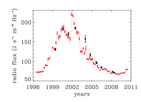
Figure 1: Mean radio flux for the observational periods in the Dynamics set (in black) and in the Structure set (in red). The error bars correspond to the error of the mean.

The ML method was applied to both observing sets and the HL only to the Dynamics set. In summary, three types of data were used in this work: (1) frequencies obtained by both ML and HL methods applied to the Dynamics set (“Dynamics ML+HL”); (2) frequencies obtained by only the ML method applied to the Dynamics set (“Dynamics ML”); and (3) frequencies obtained by only the ML method applied to the Structure set (“Structure ML”).

The estimated mode frequencies, $\nu_{nlm}$, were parameterized in terms of Clebsch-Gordan coefficients (Ritzwoller & Lavely, 1991). The central frequency, i.e., the frequency free of splitting effects, is taken to be the frequency given by $m=0$ in the parameterization. For each of these three sets, the central frequency, $\nu_{nl}$, for each time period was fitted assuming a linear and a quadratic relationship with the correspondent solar-activity index and using a weighted least-squares minimization. For a detailed description, see Rabello-Soares (2011). The solar radio 10.7 cm daily flux (NGDC/NOAA) was used as the solar-activity proxy (Figure 1).

Although, there is a very high linear correlation of the mode frequency variation with several solar-activity indices, deviations from a simple linear relation have been reported (see, for example, Chaplin et al., 2007). More recently, Rabello-Soares (2011) found some evidence of a quadratic relationship indicating a saturation at high solar activity ($\sim 350\times 10^{-22}$ J s^-1 m^-2 Hz^-1). A similar effect has been seen in frequencies at activity regions with a large surface magnetic field using ring analysis (Basu et al. 2004). The frequency shifts obtained using the quadratic fitting were used here.

Modes with a negative linear coefficient in the quadratic fitting were excluded from the present analysis. They also have a positive quadratic coefficient, indicating that they are less affected by low and medium levels of solar activity. They correspond to 5%, 11% and 16% of the modes of the Structure ML, Dynamics ML and Dynamics ML+HL sets, respectively. In the Dynamics ML+HL mode set, the excluded modes make for the lack of modes in the middle of the $l-\nu$ diagram in Figure 2. The $f$-modes obtained with the HL method (about 20 modes) have a distinctive behavior from those obtained with the ML method (see Figure 7 in Rabello-Soares, 2011). It is not clear if this behavior is an artifact of the frequency determination or not. They were excluded from our analysis.

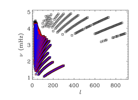
Figure 2: Modes used in the inversion for the Dynamics ML+HL, Dynamics ML and Structure ML sets are shown as black squares, red crosses and blue circles, respectively.

The solar activity minimum-to-maximum frequency shift $\delta\nu^{sc}_{nl}$ is defined as the difference between the fitted frequency at the maximum and at the minimum of solar activity. The minimum and maximum activity correspond to the Dynamics observing periods centered around April 2008 and May 2002 respectively (Figure 1). These observing periods were also used to calculate the frequency difference for the Structure set. The corresponding radio fluxes are 71 and 185 J s^-1 m^-2 Hz^-1 for both sets. The minimum-to-maximum frequency shifts $\delta\nu^{sc}_{nl}$ obtained using a linear or a quadratic fit to the solar activity are very similar.

3 The surface term

The scaled frequency differences $Q_{nl}\,\delta\nu_{nl}/\nu_{nl}$ (between two models or between the Sun and a model) can be expressed as $H_{1}(\nu_{nl}/L)+H_{2}(\nu_{nl})$, where $H_{1}$ is the contribution of the interior sound-speed difference, $H_{2}$ of the differences in the surface layers, $Q_{nl}$ is the mode inertia normalized by the inertia of a radial mode of the same frequency and $L=\sqrt{l(l+1)}$ (Christensen-Dalsgaard et al., 1989). $H_{2}$ is also called the surface term, $F_{\rm{surf}}$.

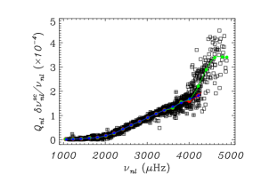
Figure 3: Scaled minimum-to-maximum frequency differences obtained using Dynamics ML+HL (black squares), Dynamics ML (black crosses) and Structure ML (small black circles) sets. Green, red and blue circles correspond to the averaged values for Dynamics ML+HL, Dynamics ML and Structure ML, respectively. The solid lines are the interpolated splines representing the surface term, $F_{\rm{surf}}$.

Figure 3 shows the scaled frequency differences between solar minimum and maximum, $Q_{nl}\,\delta\nu^{sc}_{nl}/\nu_{nl}$, obtained using Dynamics ML+HL (black squares), Dynamics ML (black crosses) and Structure ML (small black circles) sets. They are basically a function of frequency. The near-surface contribution can be removed by subtracting a smooth function of frequency, $F_{\rm{surf}}(\nu)$, from the scaled frequency shifts, thus allowing the search for structure variations in the solar interior with the solar cycle. $Q_{nl}\,\delta\nu^{sc}_{nl}/\nu_{nl}$ were averaged over 200-$\mu$Hz intervals. In each interval, outliers large than 3-$\sigma$ were removed and the weighted average calculated. The results are represented in Figure 3 as green, red and blue circles respectively for Dynamics ML+HL, Dynamics ML and Structure ML sets. A cubic spline interpolation was applied to the 17 and 21 frequency-knots for the ML and ML+HL sets, respectively (solid lines in Figure 3). Figure 4 shows the residuals after subtracting the surface term given by the splines.

Figure 4: Residuals, $Q_{nl}\,\delta\nu^{sc^{\prime}}_{nl}/\nu_{nl}$, obtained after subtracting $F_{\rm{surf}}$. The black squares, red crosses and blue circles correspond to Dynamics ML+HL, Dynamics ML and Structure ML, respectively.

4 Results

A nonasymptotic inversion technique can be applied to infer the sound speed (and density) inside the Sun using the frequency differences between the Sun and a reference solar model (e.g. Antia & Basu, 1994, and references within). Here the solar-cycle frequency shifts, $\delta\nu^{sc^{\prime}}_{nl}$, were inverted to determine the differences in sound speed between minimum and maximum solar activity inside the Sun. The inversion has been carried out using the multiplicative optimally localized averages technique (Gough, 1985). The relative frequency shifts $\delta\nu^{sc^{\prime}}_{nl}/\nu_{nl}$ are plotted in Figure 5. They are small indicating small changes in the solar structure with the solar cycle, if any at all.

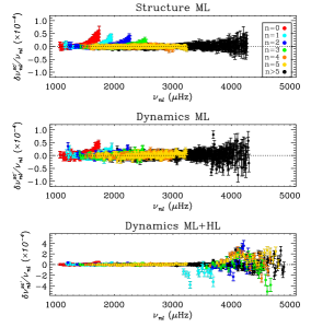
Figure 5: Relative frequency differences between solar maximum and minimum, after removing the surface term, used in the sound-speed inversion.

The inferred sound-speed differences are shown in Figure 6. The results obtained using Dynamics ML+HL (black), Dynamics ML (red) and Structure ML (blue) sets follow the same general trend. The sound-speed difference increases slowly with radius until about 0.98 $R_{\odot}$ after which it decreases sharply. The sound-speed difference is larger than 6-$\sigma$ at its maximum for all three sets. The inversion results are identical if a linear fit of the mode frequencies to the solar-activity index is used instead of a second-degree polynomial.

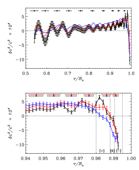
Figure 6: Inferred sound-speed differences obtained using Dynamics ML+HL (black circles), Dynamics ML (red line) and Structure ML (blue line) sets. The bottom panel shows the solution near the surface in more detail. The vertical dotted lines mark approximately the regions that correspond to positive, zero and negative sound-speed variations below an active region in relation to a quiet region obtained by ring analysis (Bogart et al., 2008).

The solution errors for the Dynamics ML+HL set are smaller by as much as 25% than for the other two sets for $r>0.85$ $R_{\odot}$ and 15% for $r<0.85$ $R_{\odot}$. Also, the averaging kernels for Dynamics ML+HL are slightly more localized close to the surface than the other two sets due to the inclusion of high-$l$ modes. In Figure 6, the averaging-kernel widths (defined as the difference between the first and third quartile points) are given by the horizontal error bars for a few selected locations. In the top panel, the horizontal bars are the same for all three sets. In the bottom panel, they are in black for Dynamics ML+HL and in red for Dynamics ML and Structure ML sets, since they are very similar. Nevertheless, the averaging kernels are well localized and have almost no side lobes for the inferred solution from 0.53 to 0.992 $R_{\odot}$ for all three sets (Figure 7). The cross-term kernel measures the influence of the contribution from density on the inferred sound speed and it is insignificant in this range (bottom panel). We did not include modes with $l<20$ in our analysis since we are not interested here in the solar deeper layers. For $r>0.992$ $R_{\odot}$, the averaging kernels become increasingly asymmetric and develop large side lobes.

Figure 7: Top: Samples of averaging kernels at five different radii near the surface for the Dynamics ML+HL set. The target radius is shown by a vertical dotted line. Bottom: Averaging kernels at $r=0.992$ $R_{\odot}$ for Dynamics ML+HL (solid line), Dynamics ML (dashed line) and Structure ML (dotted line) sets. The cross term kernel is also plotted for all three sets. It is multiplied by 100 and displaced vertically by -30 for visualization purpose.

To check that the surface term is properly removed and is not causing the observed sound-speed variation, the surface term was estimated using four times more frequency-knots than used in Figure 3 (i.e., using 50 $\mu$Hz intervals). In this case, $F_{\rm{surf}}$ is not a smooth function of frequency anymore. The inversion of the residuals is still similar to Figure 6. The maximum sound-speed variation around 0.98 $R_{\odot}$ is still statistically significant, it is larger than 4-$\sigma$ (larger than 6-$\sigma$ for the Dynamics ML+HL set).

Figure 8 shows the sound-speed difference between two different solar models (solid red line) and the correspondent inversion results (black circles) obtained using the same mode set as our observations given by Dynamics ML+HL. The inversion results are very similar using any of the other two sets. The two solar models are Model S and a model with identical physical assumptions but with a lower solar age, 4.52 Gyr, instead of 4.6 Gyr (Christensen-Dalsgaard et al., 1996). The inversion results agree very well with the true model difference for $r\leq 0.992$ $R_{\odot}$, specially taking into account the averaging kernel (dashed red line in the bottom panel).

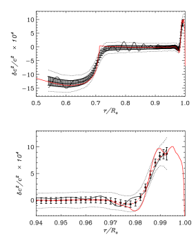
Figure 8: Sound-speed differences between two solar models through most of the solar interior (top) and, in detail, near the surface (bottom). The solid red line is the true difference between the models, while the dashed red line (bottom panel) is the difference weighted by the averaging kernels. The black circles represent the inversion results using the observed mode set for Dynamics ML+HL and the solid black line the inversion results with random noise added to the theoretical frequencies. The two dotted black lines correspond to the average of 1000 realizations plus and minus 2.5-$\sigma$.

Howe & Thompson (1996) showed that random noise in the observed mode frequency will introduce spurious oscillatory structures in the solution as a result of the correlation of the errors in the solution at different radii. The inversion result at two different radii makes use of similar data sets and their correspondent errors. The solution errors are correlated even between points farther apart than the averaging-kernel width. For examples of sound-speed error correlation, see Rabello-Soares et al. (1999) and Basu et al. (2003). To illustrate the effect of the error correlation in the inversion results presented here, it was carried out inversions of the theoretical frequency differences between the two models with noise added to them. To each frequency difference the noise was generated as normally distributed random numbers with the same standard deviation as the error in the observed data. The solid black line in Figure 8 shows the result for one realization. The spurious oscillatory structures introduced by the correlated errors, also present in Figure 6, are clearly seen. The two dotted lines correspond to the average of 1000 realizations plus and minus 2.5-$\sigma$, showing that the overall results are consistent with the estimated formal errors.

To remove the spurious oscillation in our sound-speed determination, a sum of two Gaussian functions was arbitrarily chosen as a smooth function of radius, $\widetilde{\delta}c^{2}/c^{2}(r)$. It was ‘weighted’ by the averaging kernels and fitted to the inversion results of the two Dynamics sets using a nonlinear least-square fit (red solid line in Figure 9). According to this simple model, the sound-speed difference increases with radius from around the base of the convection zone until 0.985 $R_{\odot}$ (i.e., 10 Mm below the surface) at the second helium ionization zone where $\widetilde{\delta}c^{2}/c^{2}=3.9\times 10^{-4}$. Closer to the surface, it decreases steeply with radius. It is zero at 0.990 $R_{\odot}$ (i.e., at a depth of 7 Mm) and, at 0.992 $R_{\odot}$ (or 5.5 Mm deep), $\widetilde{\delta}c^{2}/c^{2}$ = -9.2 $\times 10^{-4}$, where the sound speed at solar maximum is smaller than at solar minimum.

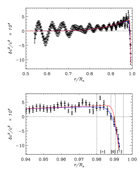
Figure 9: Black circles and diamonds are the inversion results using Dynamics ML+HL and Dynamics ML respectively. They are identical to the black and red circles in Figure 6. The red line is the smooth function, $\widetilde{\delta}c^{2}/c^{2}$, which was weighted by the averaging kernels and fitted to the inversion results of the two Dynamics sets. The blue line is $\widetilde{\delta}c^{2}/c^{2}$ weighted by the averaging kernels.

5 Discussion

Using global helioseismology, Baldner & Basu (2008) found an increase with radius in the sound-speed variation with solar cycle for $0.86<r/R_{\odot}<0.95$ (at the equator and at $15^{\circ}$ in latitude) that agrees with our results within less than 1.5-$\sigma$. Here, we found that the variation in sound speed increases until 0.985 $R_{\odot}$ after which it decreases fast with radius becoming negative for $r>0.990$ $R_{\odot}$. Posing the question of what is the physical mechanism behind this suddenly change in behavior at this particular depth.

This crossing of the sound speed at solar maximum from larger to smaller than at solar minimum is consistent in location with the crossing of the sound speed below an active region from larger to smaller than at a quiet region obtained by ring-diagram analysis (Basu et al., 2004; Bogart et al., 2008). The vertical lines in Figures 6 and 9 mark approximately the regions that correspond to Figure 9 in Bogart et al. (2008) for positive, zero and negative sound-speed variations below an active region in relation to a quiet region. This agreement indicates that the sound-speed variation in the solar interior with solar cycle might be an overall effect of the active regions local perturbation, and not a global structure change with solar activity. The estimated sound-speed variation obtained here is based on averages over the whole Sun at a particular depth and over one or more solar rotations.

The number of active regions is very well correlated with the solar activity cycle. Using the data provided by SIDC (Solar Influences Data Analysis Center of the Royal Observatory of Belgium), the daily sunspot number averaged over the maximum-activity observing period (centered around May 2002) is about 120, while during the minimum (April 2008) is less than 10. According to ring-diagram analysis, the sound-speed variation at a depth of 14 Mm (i.e., 0.98 $R_{\odot}$) below a $16^{\circ}\times 16^{\circ}$ region on the solar surface (tracked for 5.7 days) with a strong active region and with a magnetic activity index (MAI) of about 80 G in comparison to a quiet region is: $\delta c^{2}/c^{2}\approx 0.01$ (Basu et al., 2004). For a smaller sunspot with an MAI of 40 G, it is 0.05. In brief, the MAI is the average of MDI magnetograms over the same area in the solar surface and observing time as the analyzed region (for a full definition see Basu et al., 2004). Performing a “back of the envelope” calculation, if there are 11 regions with sizes of $16^{\circ}\times 16^{\circ}$ (in the front and back of the Sun) with an MAI $\gtrsim 80$ during solar maximum (or a larger number of weaker regions), the mean sound-speed variation will be $\delta c^{2}/c^{2}=4\times 10^{-4}$, i.e., the value estimated here at this depth for the maximum-to-minimum solar-cycle variation.

Time distance is another local helioseismology technique that provides information about the subsurface structure of active regions. While ring-diagram technique is based on the analysis of three-dimensional power spectra in a small region of the Sun to measure the oscillation frequencies (Hill, 1988), as in global helioseismology, time distance measures the wave travel times between different points on the surface (Duval et al., 1997). Both the ring-diagram and time-distance techniques give qualitatively similar results, revealing a characteristic two-layer seismic sound-speed structure. However, the transition between the negative and positive variations occurs at different depths: $\sim$ 4 Mm for the time-distance result, and $\sim$ $5-8$ Mm for the ring-diagram inversions. It seems that this can be explained, at least in part, by differences in the sensitivity and resolution of the two methods (see Kosovichev et al., 2011).

Recently, Ilonidis et al. (2011) using time-distance technique detected strong acoustic travel-time anomalies around 65 Mm (i.e., at 0.91 $R_{\odot}$) below the solar surface where a sunspot emerged 1 to 2 days later. These travel-time perturbations are an indication of sound-speed variations. In our simple model, $\widetilde{\delta}c^{2}/c^{2}=2.1\times 10^{-4}$ at this depth. However, the observed signal lasts only for $\sim 8$ hours and is not as strong in the layers immediately above the detected signal.

In conclusion, using acoustic mode frequencies observed by MDI/SOHO through most of solar cycle 23, we have estimated the sound-speed difference between solar maximum and minimum from 0.53 to 0.992 $R_{\odot}$. The sound-speed difference seems to increase with radius from the base of the convection zone or above until 0.985 $R_{\odot}$ (i.e., 10 Mm below the surface) at the second helium ionization zone. Closer to the surface, it decreases steeply with radius. It is zero at 0.990 $R_{\odot}$ (i.e., at a depth of 7 Mm) and, at 0.992 $R_{\odot}$ (or 5.5 Mm deep), $\widetilde{\delta}c^{2}/c^{2}=-9.2\times 10^{-4}$. The transition of the sound speed at solar maximum from larger to smaller than at solar minimum takes place at a similar depth as the transition of the sound speed below an active region from larger to smaller than at a quiet region obtained by ring-diagram analysis, suggesting that the sound-speed variation in the solar interior with solar cycle could be an overall effect of the active regions local perturbation, and not a global structure change with solar activity.

References

- Antia (2003) Antia, H. M. 2003, ApJ, 590, 567
- Antia & Basu (1994) Antia, H. M., & Basu, S. 1994, A&AS, 107, 421
- Bachmann & Brown (1993) Bachmann, K. T., & Brown, T. M. 1993, ApJ, 411, L45
- Baldner & Basu (2008) Baldner, C. S. & Basu, S. 2008, ApJ, 686, 1349
- Basu (2002) Basu, S. 2002, in Proc. SOHO 11 Symp., From Solar Min to Max: Half a Solar Cycle with SOHO, ed. A. Wilson (ESA SP-508; Noordwijk: ESA), 7
- Basu & Antia (2006) Basu, S., & Antia, H. M. 2006, in Proc. SOHO 18/GONG 2006/HELAS I, Beyond the spherical Sun, ed. K. Fletcher (ESA SP-624; Noordwijk: ESA), 128
- Basu & Mandel (2004) Basu, S., & Mandel, A. 2004, ApJ, 617, L155
- Basu et al. (2003) Basu, S., et al. 2003, ApJ, 591, 432
- Basu et al. (2004) Basu, S., Antia, H. M., & Bogart, R. S. 2004, ApJ, 610, 1157
- Bogart et al. (2008) Bogart, R. S., Basu, S., Rabello-Soares, M. C., & Antia, H. M. 2008, Sol. Phys., 251, 439
- Chaplin et al. (2007) Chaplin, W. J., Elsworth, Y., Miller, B. A., & Verner, G. A. 2007, ApJ, 659, 1760
- Christensen-Dalsgaard et al. (1989) Christensen-Dalsgaard, J., Gough, D. O., & Thompson, M. J. 1989, MNRAS, 238, 481
- Christensen-Dalsgaard et al. (1996) Christensen-Dalsgaard, J. et al. 1996, Science, 272, 1286
- Duval et al. (1997) Duvall, T. L., Jr. et al. 1997, Sol. Phys., 170, 63
- Dziembowski & Goode (2005) Dziembowski, W. A., & Goode, P. R. 2005, ApJ, 625, 548
- Eff-Darwich et al. (2002) Eff-Darwich, A., Korzennik, S. G., Jiménez-Reyes, S. J., & Pérez Hernández, F. 2002, ApJ, 580, 574
- Gough (1985) Gough, D. 1985, Sol. Phys., 100, 65
- Hathaway (2010) Hathaway, D. H. 2010, Living Rev. Solar Phys., 7, 1
- Hill (1988) Hill, F. 1988, ApJ, 333, 996
- Howe & Thompson (1996) Howe R., & Thompson M. J. 1996, MNRAS, 281, 1385
- Howe et al. (2000) Howe, R. et al. 2000, Science, 287, 2456
- Howe et al. (2005) Howe, R. et al. 2005, ApJ, 634, 1405
- Ilonidis et al. (2011) Ilonidis, S., Zhao, J., & Kosovichvev, A. 2011, Science, 333, 993
- Jain & Bhatnagar (2003) Jain, K., & Bhatnagar, A. 2003, Sol. Phys., 213, 257
- Jain et al. (2009) Jain, K., Tripathy, S. C., & Hill, F. 2009, ApJ, 695, 1567
- Korzennik (1998) Korzennik, S. G. 1998, in Proc. SOHO 6/GONG 98, Structure and Dynamics of the Interior of the Sun and Sun-like Stars, ed. S.G. Korzennik, & A. Wilson (ESA SP-418; Noordwijk: ESA), 933
- Kosovichev et al. (2000) Kosovichev, A. G., Duvall, T. L., Jr., & Scherrer, P. H. 2000, Sol. Phys., 192, 159
- Kosovichev et al. (2011) Kosovichev, A. G. et al. 2011, J. Phys. Conf. Ser., 271, 012005
- Larson & Schou (2008) Larson, T. P., & Schou, J. 2008, J. Phys. Conf. Ser., 118, 012083
- Larson & Schou (2009) Larson, T. P., & Schou, J. 2009, in Proc. GONG 2008/SOHO 21, Solar-Stellar Dynamos as Revealed by Helio- and Asteroseismology, ed. M. Dikpati et al. (ASP Conf. Ser. 416; San Francisco: ASP), 311
- Li et al. (2003) Li, L. H. et al. 2003, ApJ, 591, 1267
- Libbrecht & Woodard (1990) Libbrecht, K. G., & Woodard, M. F. 1990, Nature, 345, 779
- Lin et al. (2006) Lin, C.-H., Li, L., & Basu, S. 2006, in Proc. SOHO 18/GONG 2006/HELAS I, Beyond the spherical Sun, ed. K. Fletcher (ESA SP-624; Noordwijk: ESA), 58
- Rabello-Soares (2011) Rabello-Soares, M. C. 2011, J. Phys. Conf. Ser., 271, 012026
- Rabello-Soares & Korzennik (2009) Rabello-Soares, M. C., & Korzennik, S. G. 2009, in Proc. GONG 2008/SOHO 21, Solar-Stellar Dynamos as Revealed by Helio- and Asteroseismology, ed. M. Dikpati et al. (ASP Conf. Ser. 416; San Francisco: ASP), 277
- Rabello-Soares et al. (1999) Rabello-Soares, M. C., Basu, S., & Christensen-Dalsgaard, J. 1999, MNRAS, 309, 35
- Rabello-Soares et al. (2006) Rabello-Soares, M. C., Korzennik, S. G., & Schou, J. 2006, in Proc. SOHO 18/GONG 2006/HELAS I, Beyond the spherical Sun, ed. K. Fletcher (ESA SP-624; Noordwijk: ESA), 71
- Rabello-Soares et al. (2008) Rabello-Soares, M. C., Korzennik, S. G., & Schou, J. 2008, Sol. Phys., 251, 197
- Rhodes et al. (2002) Rhodes, E. J., Jr., Reiter, J., & Schou, J. 2002, in Proc. SOHO 11 Symp., From Solar Min to Max: Half a Solar Cycle with SOHO, ed. A. Wilson (ESA SP-508; Noordwijk: ESA), 37
- Rhodes et al. (2011) Rhodes, E. J., Jr. et al. 2011, J. Phys. Conf. Ser., 271, 012029
- Ritzwoller & Lavely (1991) Ritzwoller, M. H., & Lavely, E. M. 1991, ApJ, 369, 557
- Salabert et al. (2004) Salabert, D. et al. 2004, A&A, 413, 1135
- Scherrer et al. (1995) Scherrer, P. H. et al. 1995, Sol. Phys., 162, 129
- Schou (1992) Schou, J. 1992, Ph.D. thesis, Aarhus Univ., Denmark
- Schou (1999) Schou, J. 1999, ApJ, 523, L181
- Schou et al. (2002) Schou, J. et al. 2002, ApJ, 567, 1234
- Vorontson et al. (2002) Vorontsov, S. V. et al. 2002, Science, 296, 101
- Woodard & Noyes (1985) Woodard, M. F., & Noyes, R. W. 1985, Nature, 318, 449