Dynamical recurrence and the quantum control of coupled oscillators

Abstract

Controllability – the possibility of performing any target dynamics by applying a set of available operations – is a fundamental requirement for the practical use of any physical system. For finite-dimensional systems, such as spin systems, precise criteria to establish controllability, such as the so-called rank criterion, are well known. However most physical systems require a description in terms of an infinite-dimensional Hilbert space whose controllability properties are poorly understood. Here, we investigate infinite-dimensional bosonic quantum systems – encompassing quantum light, ensembles of bosonic atoms, motional degrees of freedom of ions, and nano-mechanical oscillators – governed by quadratic Hamiltonians (such that their evolution is analogous to coupled harmonic oscillators). After having highlighted the intimate connection between controllability and recurrence in the Hilbert space, we prove that, for coupled oscillators, a simple extra condition has to be fulfilled to extend the rank criterion to infinite-dimensional quadratic systems. Further, we present a useful application of our finding, by proving indirect controllability of a chain of harmonic oscillators.

One of the most fundamental questions in science is what kind of dynamics a given system can host. Control theory addresses this question in the light of how the dynamics of the system can change as a response to our attempts of steering it. Control theory can be applied at different levels: when dealing with computing devices, for example, one could either classify their dynamics by the primary logical operations they can perform or, at a higher and arguably more useful level, by determining what kind of programs they can run. In quantum computing the first level is typically determined by the experiments, and provides one with a description of the Hamiltonian of the system under consideration. On the other hand the second level corresponds to the set of quantum algorithms that the quantum computer is capable of running. It is at this second level that the capability for a device to perform the algorithms theorists dream of is established or disproved.

To connect the experimental and theoretical levels, one faces the problem of translating the Hamiltonian description to a description in terms of algorithms it can perform. For finite-dimensional quantum systems, for instance qubits and qudits, this translation has been accomplished in the 1970s by the development of an elegant mathematical framework dubbed as algebraic control JS ; Dalessandro . In infinite dimension, however, such a translation has been so far elusive. Roughly speaking, the problem encountered is described as follows (see Fig. 1): in finite-dimensional systems, the state space is ‘limited’, and if the quantum state evolves in one specific direction, it will eventually return to where it started. Classically this would be Poincare’s celebrated recurrence theorem, whose quantum mechanical counterpart is given in QRT . Hence, in finite dimension, there is in some sense no need to distinguish between opposite directions or, equivalently, to specify the direction of time. For control theory this allows one to develop a picture in which time is fully eliminated. Single-directed movement in infinite-dimensional systems however can carry an ‘intrinsic clock’, e.g. distance travelled from some initial state, and time cannot be eliminated.

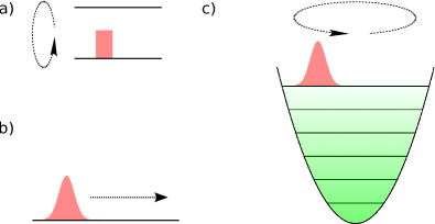
Figure 1: In finite dimensions, quantum systems recur (a), while, in infinite dimensions, single-directed movement can carry an ‘intrinsic clock’ and systems do not recur anymore (b). However, under certain conditions, we prove that harmonic oscillator systems (c) can recur as if they were finite-dimensional.

Now in order to assess quantum control of an infinite-dimensional system, our question is: do all infinite-dimensional systems have an intrinsic clock? A counterexample is given by harmonic oscillators: just by looking at the system state of an oscillator, one cannot tell how long it has been running from any specific initial state. Hence, there is hope to perform the same time elimination and reach an easy description of operations that can be performed in quantum harmonic oscillators. Note that these systems are not mere theoretical curiosities. The control of the infinite-dimensional degrees of freedom of light, trapped particles, nano- and opto-mechanical oscillators, superconductors, Bose-Einstein condensates, and of collective spins of atomic vapors or solid-state devices are all of major technological interest, and the primary way to address most of such degrees of freedom is the manipulation of quadratic Hamiltonians, which correspond to descriptions in terms of quantum harmonic oscillators light ; ions1 ; ions2 ; nano ; opto ; ensembles . We will see a specific example concerning the control of arrays of trapped ions at the end of the Letter.

In this letter, we prove that a restrictive condition has to be fulfilled in order to assess the controllability of quantum harmonic oscillator networks. We shall observe that such systems share substantial similarities with finite-dimensional dynamics, which explains the success of previous numerical results rabitz . We also demonstrate the potential impact of our findings by showing how indirect control methods Daniel , developed previously for spin systems only, can also be applied to oscillators, possibly leading to resource efficient cooling and control protocols. We start by presenting the basic notions of the algebraic control, revisiting the proof of the Lie algebra rank criterion JS ; Dalessandro and finding why it fails to be sufficient for the controllability of generic infinite-dimensional systems. Then we will focus on quadratic bosonic Hamiltonians, which give rise to the so-called Gaussian operations, and we will determine a condition such that the rank criterion will still be sufficient for controllability in the restricted Gaussian sense. In the end, we will present an example relevant to arrays of trapped ions and to chain of nano-mechanical oscillators, where this condition is fulfilled and where local controllability can be proven by applying our general analysis.

Algebraic control - Let us start by reviewing a finite-dimensional control setup in quantum physics. Suppose an experimentalist succeeds in setting up a system described by the Hamiltonian

$$H(t)=H_{0}+\sum_{k=1}^{m}f_{k}(t)H_{k},$$ (1)

where the $H_{k}$ are a set of controlling Hamiltonians that can be switched on and off. The Schrödinger equation for the time evolution operator $U$ then reads

$$\frac{dU}{dt}=-iH(t)\>U\qquad U(0)=\mathbbm{1}.$$ (2)

The main goal of a control theorist is to determine which quantum algorithms, i.e. which unitary operators $U$, the experimentalist can, in principle, achieve by setting the right switching times for the $f_{k}$.
In this Letter we are interested in controlling systems described as coupled oscillators, thus we need to introduce some additional notation and terminology. We shall consider an $n$-mode bosonic system, described by $n$ pair of quadrature operators $q_{j}$ and $p_{j}$ satisfying the canonical commutation relation $[q_{k},p_{l}]=i\delta_{k,l}$. By introducing the vector of operators $R^{T}=(q_{1},p_{1},\dots,q_{n},p_{n})$, the commutation relation can be written as $[R_{k},R_{l}]=i\Omega_{kl}$ where $\Omega$ is the $(2n)\times(2n)$ symplectic form whose matrix elements are $\Omega_{jk}=\delta_{j+1,k}[1-(-1)^{j}]/2-\delta_{j,k+1}[1+(-1)^{j}]/2$ in terms of Kronecker deltas $\delta_{j,k}$.
In particular we will consider systems described and controlled by Hamiltonians that are bilinear in the quadrature operators, i.e. that can be written as $H=(1/2)\sum_{k,l}A_{kl}R_{k}R_{l}$ where $A$ are real and symmetric $2n\times 2n$ matrices. The corresponding evolution operators in the infinite-dimensional Hilbert space, defined as $U=e^{-iHt}$, are the so-called Gaussian unitary operations since they preserve the Gaussian character of quantum states Gaussians1 ; Gaussians2 . If we consider the Heisenberg evolution for the quadrature operators vector $R$, we obtain the equation $U^{{\dagger}}RU=SR$ where $S=e^{-A\Omega t}$ is a $2n\times 2n$ matrix belonging to the real symplectic group $Sp(2n,\mathbbm{R})$ satisfying the equation $S\Omega S^{T}=\Omega$ agarwal . Then, restricting to quadratic Hamiltonians, there is a one-to-one correspondence between the evolution operator in the infinite-dimensional Hilbert space $U$ and the finite-dimensional matrix $S$, in particular they correspond to different representations of the real symplectic group Arwind . As a consequence Eq. (2) can be recast in terms of the symplectic representation, providing one with the following evolution equation

$$\frac{dS}{dt} =G(t)S\qquad S(0)=\mathbbm{1},$$ (3)

where, as pointed out above, $S$ is no longer unitary, and $G(t)=-(A^{(0)}+\sum_{k=1}^{m}f_{k}(t)A^{(k)})\Omega$ is no longer anti-hermitian. In this framework, the main goal of the control theorist can be summed up by the following question: which symplectic time-evolutions $S$ are achievable by controlling $G(t)$ via the functions $f_{k}(t)$?
Because the solutions of Eq. (3) are elements of matrix groups, one can apply the beautiful framework of Lie groups to tackle such questions. Let us suppose that, by setting the control functions equal to constant values in $G(t)$, we can identify a set $\mathcal{E}=\{\widetilde{G}_{1},\cdots,\widetilde{G}_{m}\}$ of linearly independent generators of a Lie algebra $\mathcal{L}$. This assumption is known as the Lie algebra rank criterion. Its relevance is due to the fact that, if the corresponding Lie group $\mathcal{G}=e^{\mathcal{L}}$ is a subset of a compact group, then all its elements can be implemented with arbitrary precision and the system is said to be controllable. The Lie algebra rank criterion is an easy and extremely powerful criterion for controllability and works well for finite-dimensional unitary gates since they are subgroups of the compact group $SU(n)$. On the other hand the solutions of (3) no longer enjoy this property, so we cannot apply the rank criterion directly.

Why and where is the compactness used to prove that the rank criterion is sufficient for controllability? Given a generic Lie group $\mathcal{G}$, a set $\mathcal{E}=\{\widetilde{G}_{1},\cdots,\widetilde{G}_{m}\}$ of linearly independent generators of the corresponding Lie algebra, and an element $K\in\mathcal{G}$, one can write

$$K =e^{\widetilde{G}_{1}t_{1}}e^{\widetilde{G}_{2}t_{2}}\cdots e^{\widetilde{G}_{n}t_{n}}$$

$$\textrm{with}\>\>\widetilde{G}_{j}\in\mathcal{E}\>\>\textrm{and}\>\>t_{j}\in\mathbbm{R}.$$ (4)

In principle, in the expression above, there will be some exponentials involving negative times $t_{j}$, while, if we want $K$ to be reachable by control, we need all the times to be positive so that every exponential in the product corresponds to an evolution described by Eq. (3) and obtained by setting the control functions equal to certain constant values. As shown in JS ; Dalessandro ; Dalessandro2 , the compactness of the Lie group is a sufficient condition to switch the sign from negative to positive time: let $\widetilde{G}$ be one of the generators of $\mathcal{L}$ and consider a negative time $t<0$. If $\mathcal{G}=e^{\mathcal{L}}$ is compact, then a sequence of positive times $t_{k}>0$ always exists such that

$$\lim_{k\rightarrow\infty}e^{\widetilde{G}t_{k}}=e^{\widetilde{G}t}.$$ (5)

In other words, for a given $\epsilon>0$ and time $t<0$, we can always find a positive time $\tau>0$, such that, for a given matrix norm, $\lVert e^{\widetilde{G}\tau}-e^{\widetilde{G}t}\rVert<\epsilon$.
One should also notice that this condition is equivalent to saying that at a certain time, the evolution operator recurs to the identity, that is, recurrence is a necessary and sufficient condition to revert the sign from negative to positive times. When one deals with non-compact groups, the possibility to switch from negative to positive times is in general lost. A simple and visually clear example in this sense is given by the squeezing operation in phase-space BR : if we continuously apply the squeezing operation, the state gets more and more squeezed and recurrence is never achieved.
However we will show in the following that for coupled harmonic oscillators, even considering non-compact Lie groups, recurrence takes place with arbitrary precision if an additional condition on the system’s Hamiltonian is met. Since, as we pointed out before, in the proof of the rank criterion, compactness is used only to revert the sign of time in evolution operators, if one is able to achieve this goal by imposing other different physical and mathematical constraints, then the rank criterion remains necessary and sufficient to prove that the reachable set is dense in the Lie group being considered.

Controllability of quadratic Hamiltonians - Previously we showed that, given a system described by Eq. (20), a linear control problem for the unitary operator $U$ is defined by the Schrödinger equation as in Eq. (2). If we consider Hamiltonians bilinear in quadrature operators such that

$$H_{k}=\frac{1}{2}\sum_{s,t}A_{st}^{(k)}R_{s}R_{t}\qquad k=\{0,\dots,m\},$$ (6)

the corresponding unitary operators $U$ are infinite-dimensional matrices; however we can consider the equivalent control problem, with the form of Eq. (3), for the finite-dimensional evolution matrix $S$ as

$$\frac{dS}{dt}=-A(f,t)\Omega\>S\qquad S(0)=\mathbbm{1}$$ (7)

where $A(f,t)=A^{(0)}+\sum_{k=1}^{m}f_{k}(t)A^{(k)}$.
The two evolution equations are equivalent and we will focus for the moment on the finite-dimensional representation in Eq. (7). The symplectic group $Sp(2n,\mathbbm{R})$ is a non-compact group and thus one cannot apply the rank criterion to assess the controllability of the system. Our main result, contained in the following theorem, shows that if we can identify a set of linearly independent generators of the symplectic algebra $\mathcal{L}=sp(2n,\mathbbm{R})$, such that the corresponding $\widetilde{A}^{(k)}$ are positive definite, one can achieve recurrence with arbitrary precision, and thus the rank criterion will still be a sufficient condition for controllability.

Theorem: If $A$ is a positive (negative) definite matrix then,

$$\forall\>\epsilon>0\>\>\textrm{and}\>\>\forall\>T>0,\>\>\exists\>\tau>T\>\>\textrm{such that}\>\>\lVert e^{-A\Omega\tau}-\mathbbm{1}\rVert<\epsilon$$

where we considered the Euclidean matrix norm $\lVert M\rVert=\sqrt{\hbox{Tr}[M^{\dagger}M]}$.
Proof: If $A$ is a positive definite matrix, because of Williamson theorem Williamson , we can write $A=VDV^{T}$ where $D={\rm diag}\{\nu_{1},\nu_{1},\dots,\nu_{N},\nu_{N}\}$, $\nu_{j}\in\mathbbm{R}^{+}$ and $V$ belongs to $Sp(2n,\mathbbm{R})$. This implies that $V^{T}\Omega=\Omega V^{-1}$ and thus we obtain $A\Omega=VD\Omega V^{-1}$.
The matrix $D\Omega$ is a normal matrix diagonalized by a unitary matrix $U$, such that $D\Omega=UD^{\prime}U^{{\dagger}}$ with $D^{\prime}={\rm diag}\{+i\nu_{1},-i\nu_{1},\dots,+i\nu_{N},-i\nu_{N}\}.$ Then we have

$$A\Omega =VUD^{\prime}U^{{\dagger}}V^{-1}=WD^{\prime}W^{-1}$$ (8)

that is $A\Omega$ has pure imaginary eigenvalues and is diagonalized by the matrix $W=VU$. As a consequence, we can write the matrix $S(t)=e^{-A\Omega t}$ as

$$S(t)=WE(t)W^{-1}$$ (9)

with $E(t)={\rm diag}\{e^{-i\nu_{1}},e^{i\nu_{1}},\dots,e^{-i\nu_{n}},e^{i\nu_{n}}\}$, which leads to

$$\lVert S(t)-\mathbbm{1}\rVert =\lVert W(E(t)-\mathbbm{1})W^{-1}\rVert$$ (10)

$$\leq\lVert W\rVert\>\lVert W^{-1}\rVert\>\lVert E(t)-\mathbbm{1}\rVert.$$ (11)

The matrix $W$ is independent on time $t$, and thus $\lVert W\rVert\>\lVert W^{-1}\rVert=K$ is constant. Let us consider the remaining term

$$\lVert E(t)-\mathbbm{1}\rVert =\sqrt{\hbox{Tr}[|E(t)-\mathbbm{1}|^{2}]}$$ (12)

$$=\left(2\sum_{k=1}^{n}|e^{-i\nu_{k}t}-1|^{2}\right)^{1/2}.$$ (13)

It is easy to check that $\lVert E(t)-\mathbbm{1}\rVert$ is a sum of trigonometric exponential functions and thus is a quasi-periodic function. Because of this property, a time $\tau>T$ exists, such that $\lVert E(\tau)-\mathbbm{1}\rVert$ is close to zero with arbitrary precision bohr . In particular, for a given $\epsilon>0$, we can choose a time $\tau$ such that $\lVert E(\tau)-\mathbbm{1}\rVert\leq\epsilon/K$ and then obtain the thesis $\lVert S(\tau)-\mathbbm{1}\rVert\leq\epsilon$. $\blacksquare$
It is worth also to notice that our result can be extended to semi-definite matrices $A$’s such that $\Omega A$ is diagonalisable, but it cannot be extended to generic semi-definite $A$’s. For instance, the Hamiltonian $H=p^{2}$ for a single degree of freedom would not recur.

This theorem assures that if, by properly choosing the control functions $f_{k}(t)$ in the Hamiltonian given in Eq. (20), we can identify a set of linearly independent generators of the symplectic group, such that the corresponding matrices $\widetilde{A}^{(k)}$ are positive (negative) definite, then we can always revert the sign of negative times in the expression corresponding to Eq. (4). As a consequence the Lie algebra rank criterion remains a necessary and sufficient condition to asses the controllability of the symplectic group, even if the group is not compact, and thus can be used to assess which Gaussian operations can be realized given a certain control problem as indicated in Eq. (7).
On a more fundamental level, our argument highlights a hitherto unnoticed connection between the normal mode decomposition of positive definite quadratic Hamiltonians – formally an implication of the Williamson theorem – and the controllability of sets of coupled oscillators. This connection is bridged by the notion of dynamical recurrence which, regardless of the infinite-dimensionality of the Hilbert space, is always guaranteed for positive definite quadratic Hamiltonians. The generality of our result makes it at first easy to overlook its potential impact: the applicability of quantum control to continuous-variable systems paves the way to vastly improving fidelities of current experiments as well as using control more efficiently. This fact can be clearly seen in the simple but quite surprising example we provide below, where our result is used to simplify the controllability properties of a large harmonic oscillator network.

Local controllability of a quadratic harmonic oscillator chain - One of the most important requirements in quantum information and quantum computation is to dynamically address and control individual interacting systems. From an experimental point of view, it is also desirable to have complete control on a large network by acting only on a small part of it. Indirect control has been already proved for qubit systems Daniel , while, regarding networks of harmonic oscillators, it has been recently shown, for instance, that by probing only one site of the network, one can reconstruct the full quantum state of the system tom . Here we use our theorem to prove the controllability of a chain of harmonic oscillators, where only one or few sites of the chain are accessible. This kind of example is relevant if we think, for example, of an array of interacting trapped ions, where in principle one can implement Gaussian operations by addressing single ions and manipulating their trapping frequencies ions2 ; alessioIons .
Let us start by defining the bosonic mode operators $a_{j}=(q_{j}+ip_{j})/\sqrt{2}$ and $a_{j}^{\dagger}=(q_{j}-ip_{j})/\sqrt{2}$, satisfying the commutation relation $[a_{i},a_{j}^{{\dagger}}]=\delta_{ij}$. Let us consider an $n$-mode bosonic chain, described by a Hamiltonian as in Eq. (20). In particular the always-on Hamiltonian reads

$$H_{0} =\omega\sum_{j=1}^{n}\left(a_{j}^{{\dagger}}a_{j}+\frac{1}{2}\right)+g_{1}\sum_{j=1}^{n-1}(a_{j}a_{j+1}^{\dagger}+h.c.)+$$

$$\>\>\>+g_{2}\sum_{j=1}^{n-1}(a_{j}a_{j+1}+h.c.).$$ (14)

where, for the sake of simplicity, we consider all the oscillators having with the same frequency $\omega$. If we consider $g_{1}=g_{2}$, this corresponds to the $q_{j}q_{j+1}$ coupling, which is the most common between the harmonic oscillators’ interactions. From now on we will consider the renormalized coupling constants $\widetilde{g}_{j}=g_{j}/\omega$ and assume that they are both positive; a sufficient condition for the positivity of $H_{0}$ (for every number of bosons in the chain $n$) is $\widetilde{g}_{1}+\widetilde{g}_{2}<1/2$. We consider as the controlling Hamiltonians, a local phase-rotation and a local squeezing term on the first mode of the chain only, i.e.:

$$H_{1}=\omega_{1}\left(a_{1}^{\dagger}a_{1}\right)\>\>\>\textrm{and}\>\>\;H_{2}=\chi(a_{1}^{2}+a_{1}^{{\dagger}2})\>.$$ (15)

We prove that, by denoting with $\mathcal{L}$ the symplectic algebra,

$$\mathcal{L}=\langle iH_{0},iH_{1},iH_{2}\rangle_{[\cdot,\cdot]},$$ (16)

that is, by computing all possible commutators of these operators, of any order, and their linear combinations, we can obtain all the elements of $\mathcal{L}$ (details of the proof can be found in the Supplemental Material). Since the Lie algebra is a vector space, any set of linearly independent linear combinations of the above operators satisfies the rank criterion. We have then to show that, by properly setting the control functions $f_{k}(t)$, we can identify one of these sets, such that the corresponding matrices $\widetilde{A}^{(k)}$ are positive definite. There are in principle infinite choices, in particular it is easy to check that the following set fulfils all the conditions above

$$\widetilde{H}_{0} =H_{0}$$ (17)

$$\widetilde{H}_{1} =H_{0}+\alpha H_{1}\qquad \alpha\omega_{1}>0$$ (18)

$$\widetilde{H}_{2} =H_{0}+\beta H_{1}+\delta H_{2}\qquad 0<\delta\chi<\beta\omega_{1}\>.$$ (19)

In practice, this example is directly relevant to arrays of trapped ions and chains of nano-mechanical oscillators. For instance, in the case of the transverse ionic modes, local controls analogous to (22) could be obtained by manipulating the local trapping frequencies, as detailed in alessioIons and realised in ions2 (analogous forms of control have been envisaged for opto-mechanical setups as well mari ). Note also that even restricted local control might suffice for certain manipulations, depending on the desired tasks. For instance, as a side product of the proof reported in the Supplemental Material, one can show that, if the local control is restricted to phase rotations generated by $H_{1}$, the whole symplectic algebra is not achievable, but all the passive operations, comprising beam-splitters and local phase rotations can be realized. This would allow one to implement, for example, cooling protocols based on swapping excitations between sites of the array.

Conclusions - While the general control theory of infinite-dimensional systems remains hard, we have found a surprisingly simple solution for the case of quadratic interactions of coupled harmonic oscillators. To demonstrate the applicability of our result, we have also discussed its application to indirect control (and, potentially, cooling) of chains of oscillators.
It is worth mentioning that proving controllability and finding an actual control pulse are completely distinct tasks. For instance, using the quantum recurrence theorem on the theory level is useful, but for a control pulse one could not rely on it, as the recurrence and hence the resulting pulses would take far too much time. This is well understood and typically overcome by using numerical routines to optimize the pulses. In our case, a similar point arises regarding the requirement of positive (negative) definiteness of the Hamiltonian, which was used as a sufficient element of the proof. In an actual pulse sequence, it could be beneficial to use non-positive or negative definite Hamiltonians in order to achieve faster control.
Last, but not least, let us remark that the dynamics of classical systems governed by quadratic Hamiltonians is also described by the symplectic group of canonical transformations: our finding hence applies, as it stands, to the controllability of classical, as well as quantum harmonic oscillators.

Acknowledgements - MSK acknowledges support from UK EPSRC and MGG acknowledges a fellowship support from UK EPSRC (grant EP/I026436/1) . Part of this work was carried out while DB held the UK EPSRC grant EP/F043678/1 at Imperial College London.

I Supplemental material

I.1 Proof of rank criterion for harmonic oscillator chain

Here we consider the control problem defined by the Hamiltonian

$$H(t)=H_{0}+\sum_{k=1}^{m}f_{k}(t)H_{k},$$ (20)

where the always-on Hamiltonian reads

$$H_{0} =\omega\sum_{j=1}^{n}\left(a_{j}^{{\dagger}}a_{j}+\frac{1}{2}\right)+g_{1}\sum_{j=1}^{n-1}(a_{j}a_{j+1}^{\dagger}+h.c.)+$$

$$\>\>\>+g_{2}\sum_{j=1}^{n-1}(a_{j}a_{j+1}+h.c.),$$ (21)

the local controlling Hamiltonians are

$$H_{1}=\omega_{1}\left(a_{1}^{\dagger}a_{1}\right)\>\>\>\textrm{and}\>\>\;H_{2}=\chi(a_{1}^{2}+a_{1}^{{\dagger}2})\>,$$ (22)

and $a_{j}$ and $a_{j}^{\dagger}$ are $n$ pairs of bosonic operators satisfying the commutation relation $[a_{j},a_{k}]=\delta_{j,k}$.
In the following we prove that the Lie algebra rank criterion for this system is fulfilled, that is, by denoting with $\mathcal{L}$ the symplectic algebra, then

$$\mathcal{L}=\langle iH_{0},iH_{1},iH_{2}\rangle_{[\cdot,\cdot]}.$$ (23)

We will work with the infinite-dimensional representation of the real symplectic group, where the basis of the corresponding Lie algebra reads

$$\mathcal{L}= \{i(a_{j}a_{k}^{\dagger}+a_{j}^{\dagger}a_{k}),a_{j}a_{k}^{\dagger}-a_{j}^{\dagger}a_{k},,$$

$$i(a_{j}^{\dagger}a_{k}^{\dagger}+a_{j}a_{k}),a_{j}^{\dagger}a_{k}^{\dagger}-a_{j}a_{k}\}$$

$$\textrm{with}\>\>j,k=1,\dots,n\>.$$ (24)

Proving the Lie algebra rank criterion corresponds to showing that by computing all possible commutators of the control operators $H_{k}$, of any order and their linear combinations, we can generate all the elements of the basis of the algebra listed above. For the sake of simplicity we will prove it by considering the case $g_{1}=g_{2}$ in the Hamiltonian $H_{0}$ (21); this corresponds to considering a $q_{j}q_{j+1}$ coupling between the sites of the chain, while the most general case (which comprises also the rotating-wave approximation case where $g_{2}=0$ ) can be proved following the same line of reasoning. We start by showing that we can generate all the elements corresponding to the two first sites of the chain:

$$S_{a}^{(1)} =\frac{1}{2}[iH_{2},iH_{1}]=a_{1}^{{\dagger}2}-a_{1}^{2}$$ (25)

$$O_{1} =[iH_{0},iH_{1}]=a_{1}^{\dagger}a_{2}^{\dagger}+a_{1}^{\dagger}a_{2}-a_{1}a_{2}^{\dagger}-a_{1}a_{2}$$ (26)

$$O_{2} =[iH_{1},O_{1}]=i(a_{1}^{\dagger}a_{2}^{\dagger}+a_{1}^{\dagger}a_{2}+a_{1}a_{2}^{\dagger}+a_{1}a_{2})$$ (27)

$$R^{(12)}_{a} =\frac{1}{2}\left[\left([O_{1},iH_{0}]+2O_{2}\right),iH_{1}\right]=a_{1}^{\dagger}a_{2}-a_{1}a_{2}^{\dagger}$$ (28)

$$T_{a}^{(12)} =O_{1}-R^{(12)}_{a}=a_{1}^{\dagger}a_{2}^{\dagger}-a_{1}a_{2}$$ (29)

$$S_{a}^{(2)} =[T_{a}^{(12)},R_{a}^{(12)}]+S_{1}^{(1)}=a_{2}^{{\dagger}2}-a_{2}^{2}$$ (30)

$$T_{b}^{(12)} =[O_{1}-R_{a}^{(12)},iH_{1}]=i(a_{1}^{\dagger}a_{2}^{\dagger}+a_{1}a_{2})$$ (31)

$$O_{3} =[iH_{1},O_{1}-2R_{a}^{(12)}]$$

$$=i(a_{1}^{\dagger}a_{2}^{\dagger}-a_{1}^{\dagger}a_{2}-a_{1}a_{2}^{\dagger}+a_{1}a_{2})$$ (32)

$$R_{b}^{(12)} =\frac{1}{2}(O_{2}-O_{3})=i(a_{1}^{\dagger}a_{2}+a_{1}a_{2}^{\dagger})$$ (33)

$$P^{(2)} =\frac{1}{2}\left(2iH_{1}+[R_{b}^{(12)},R_{a}^{(12)}]\right)=ia_{2}^{\dagger}a_{2}$$ (34)

$$S_{b}^{(2)} =[P^{(2)},S_{a}^{(2)}]=i(a_{2}^{{\dagger}2}+a_{2}^{2})\>.$$ (35)

The operators $P^{(2)}$, $S_{a}^{(1)}$, $S_{a}^{(2)}$, $S_{b}^{(2)}$, $T_{a}^{(12)}$, $T_{b}^{(12)}$, $R_{a}^{(12)}$, $R_{b}^{(12)}$, together with the local control operators $iH_{k}$, complete all the operators corresponding to the first two sites. Because of the symmetry of $H_{0}$, we can proceed in the same way for all the operators belonging to the neighbouring sites. Then, to obtain the two-mode long-distance operators, one can easily show that

$$[i(a_{k}^{\dagger}a_{l}+a_{k}a_{l}^{{\dagger}}),a_{j}a_{k}^{\dagger}-a_{j}^{\dagger}a_{k}]=i(a_{j}^{\dagger}a_{l}+a_{j}a_{l}^{\dagger})$$ (36)

and analogue commutators for the remaining terms. The proof is hence complete. $\blacksquare$

References

- (1) V. Jurdjevic and H. Sussmann, J. Diff. Eqns. 12, 313 (1972).
- (2) D. D’Alessandro, Introduction to Quantum Control and Dynamics, (Taylor & Francis, Boca Raton, 2008).
- (3) P. Bocchieri and A. Loinger, Phys. Rev. 107, 337 (1957).
- (4) Z. Y. Ou, S. F. Pereira, H. J. Kimble, and K. C. Peng, Phys. Rev. Lett. 68, 3663 (1992); A. Furusawa, J. L. Sørensen, S. L. Braunstein, C. A. Fuchs, H. J. Kimble, and E. S. Polzik, Science 282, 706 (1998); H. Yonezawa, T. Aoki, and A. Furusawa, Nature 431, 430 (2004).
- (5) D. Leibfried, R. Blatt, C. Monroe, and D. J. Wineland, Rev. Mod. Phys. 75, 281 (2003).
- (6) K. R. Brown, C. Ospelkaus, Y. Colombe, A. C. Wilson, D. Leibfried, and D. J. Wineland, Nature 471, 196 (2011).
- (7) J. Eisert, M. B. Plenio, S. Bose, and J. Hartley, Phys.Rev. Lett. 93, 190402 (2004).
- (8) J. D. Thompson, B. M. Zwickl, A. M. Jayich, Florian Marquardt, S. M. Girvin, and J. G. E. Harris, Nature 452, 72 (2008); M. Ludwig, K. Hammerer, and F. Marquardt, Phys. Rev. A 82, 012333 (2010).
- (9) K. Hammerer, A. S. Sørensen, and E. S. Polzik, Rev. Mod. Phys. 82, 1041 (2010).
- (10) R. Wu, R. Chakrabarti and H. Rabitz, Phys. Rev. A 77, 052303 (2008).
- (11) D. Burgarth, S. Bose, C. Bruder, V. Giovannetti, Phys. Rev. A 79, 060305(R) (2009).
- (12) A. Ferraro, S. Olivares and M. G. A. Paris, Gaussian States in Quantum Information, (Bibliopolis, Napoli, 2005).
- (13) J. Eisert, M. B. Plenio, Int. J. Quant. Inf. 1, 479 (2003).
- (14) H. Huang and Girish S. Agarwal, Phys. Rev. A 49, 52 (1994).
- (15) Arvind, B. Dutta, N. Mukunda and R. Simon, PRAMANA 45, 471 (1995); preprint: arXiv:quant-ph/9509002.
- (16) D. D’Alessandro, J. Phys. A: Math. Theor. 42, 395301 (2009).
- (17) S. M. Barnett and P. M. Radmore, Methods in theoretical quantum optics, (Oxford University Press, 1997).
- (18) T. Tufarelli, A. Ferraro, M. S. Kim and S. Bose, Phys. Rev. A 85, 032334.
- (19) A. Serafini, A. Retzker and M. B. Plenio, New Journal of Physics 11 , 023007 (2009); Quantum Inf. Process. 8, 619 (2009).
- (20) A. Mari and J. Eisert, Phys. Rev. Lett. 103, 213603 (2009).
- (21) J. Williamson, Am. J. Math. 58, 141 (1936).
- (22) H. Bohr, Almost-periodic functions, (Chelsea, reprint, 1947).

References

- (1) V. Jurdjevic and H. Sussmann, J. Diff. Eqns. 12, 313 (1972).
- (2) D. D’Alessandro, Introduction to Quantum Control and Dynamics, (Taylor & Francis, Boca Raton, 2008).