Low- and High-Energy Expansion of Heavy-Quark Correlators at Next-To-Next-To-Leading Order

Abstract

We calculate three-loop corrections to correlation functions of heavy-quark currents in the low- and high-energy regions. We present 30 coefficients both in the low-energy and the high-energy expansion of the scalar and the vector correlator with non-diagonal flavour structure. In addition we compute 30 coefficients in the high-energy expansion of the diagonal vector, axial-vector, scalar and pseudo-scalar correlators. Possible applications of our new results are improvements of lattice-based quark-mass determinations and the approximate reconstruction of the full momentum dependence of the correlators.

,

1 Introduction

The precise determination of the fundamental parameters of the Standard Model (SM) is of utmost importance to pin down the fundamental interactions of the elementary particles and to establish deviations from the SM. Three especially interesting parameters, namely the strong coupling constant and the masses of charm and bottom quarks, can be determined with high accuracy from correlators of heavy-quark currents by comparing their moments with experimental data using sum rules [1, 2]. Conventionally, moments from the low-energy expansion have been used for this purpose [3, 4, 5, 6, 7, 8], but also methods relying on high-energy moments have been shown to yield quite accurate results [9].

As an alternative to experimental data also lattice simulations can be used in order to compute moments of two-point functions. Thanks to significant improvements in the last years results can be obtained not only for the charm-quark mass and the strong coupling constant [10], but also for the bottom-quark mass [11].

Aside from these determinations, quark-current correlators have a number of additional phenomenological applications. Two examples are the sum-rule determinations of heavy-meson decay constants and $\alpha_{s}(m_{\tau})$ (for recent works see e.g. Refs  [12, 13, 14, 15]). While the former requires – among other ingredients – the low-energy expansion of the respective correlator, the latter uses the absorptive part above the production threshold.

In this work we consider correlators of quark currents with various different Lorentz structures. Furthermore we distinguish between diagonal and non-diagonal correlators. The diagonal correlators are defined through

$$\Pi_{\mathrm{D}}^{X}(q)=i\int e^{iqx}\langle 0|J^{X}(x)J^{X}(0)|0\rangle\mathrm{d}x\,,$$ (1)

with the currents $J^{X}(x)$ given by

$$J^{X}(x)=\bar{\psi}(x)\Gamma^{X}\psi(x)\,.$$ (2)

The non-diagonal correlators are defined in analogy by

$$\Pi_{\mathrm{ND}}^{X}(q)=i\int e^{iqx}\langle 0|j^{X}(x)j^{X}(0)|0\rangle\mathrm{d}x\,,$$ (3)

with the currents $j^{X}(x)$ given by

$$j^{X}(x)=\bar{\psi}(x)\Gamma^{X}\chi(x)\,.$$ (4)

Here $\psi$ denotes a heavy quark while $\chi$ stands for a massless one. The scalar, pseudo-scalar, vector and axial-vector currents are defined through the Dirac structures $\Gamma^{X}=1,i\gamma_{5},\gamma_{\mu},\gamma_{\mu}\gamma_{5}$ ($X=s,p,v,a$), respectively. Note that in the case of the non-diagonal correlators $\Pi_{\mathrm{ND}}^{s}=\Pi_{\mathrm{ND}}^{p}$ and $\Pi_{\mathrm{ND}}^{v}=\Pi_{\mathrm{ND}}^{a}$ hold.

For the determination of the quark masses from experimental data only the diagonal vector correlator $\Pi_{\mathrm{D}}^{v}$ can be used while it is in principle possible to use all diagonal and non-diagonal correlators in combination with lattice simulations.

Current-current correlators have already been extensively studied in the literature. The two-loop corrections to the diagonal vector correlator have been calculated in [16], the corresponding corrections for the non-diagonal one in [17]. At three loops the leading terms of the low- and high-energy expansion have been determined in [18, 19]. For the diagonal correlators many terms in the low-energy expansion have been computed in [20, 21]. At four loops the leading terms in the low-energy expansion of various currents have been calculated in [22, 23, 4, 24, 25]. In the high-energy region the expansion at four-loop order has been obtained in [26]. In [27] effects of a second massive quark have been taken into account at three-loop order. Collecting the available information for the correlators at three and four loops, the full momentum dependence has been approximated using Padé approximations and Mellin-Barnes inspired methods [28, 18, 29, 30, 31, 32]. In this paper we complete the calculation of the low- and high-energy expansion of diagonal and non-diagonal heavy-quark correlators using an improved method for the calculation.

In Section 2 we present the details of the calculation. In Section 3 we present explicit results for the non-diagonal vector correlator in numerical form and discuss the convergence of the expansions. The analytical results for all correlators can be found on the web page
http://www-ttp.particle.uni-karlsruhe.de/Progdata/ttp11/ttp11-25/.

2 Details of the calculation

The calculation is organized as follows. The diagrams are generated using qgraf [33] and are subsequently mapped onto a small set of 11 topologies (cf. Fig. 1) using q2e and exp [34]. After the application of suitable projectors the resulting scalar integrals are reduced to the master integrals shown in Fig. 2 using integration-by-parts identities [35, 36] implemented in the program Crusher [37]. The resulting expression which still contains the full dependence on both the external momentum square $q^{2}$ and the heavy-quark mass $m$ is then – lacking an analytical result for the master integrals – expanded in the energy region of interest as explained in more detail below. The expanded master integrals are combined in a FORM [38] program in order to obtain the final expressions valid in either the low-energy or the high-energy region. For further use the low- and high-energy expansions of all master integrals can be obtained from the web site http://www-ttp.particle.uni-karlsruhe.de/Progdata/ttp11/ttp11-25/masters/.

Figure 1: Three-loop master topologies needed for the calculation of the non-diagonal and diagonal correlators. Solid lines denote massive propagators while dotted lines represent massless ones.

Figure 2: All master integrals needed for the calculation of the diagonal and non-diagonal correlators up to three loops. Solid lines denote massive propagators while dotted lines represent massless ones. A dot on a line denotes a squared propagator.

The coupling constant $\alpha_{s}$ is renormalized in the $\overline{\text{MS}}$ scheme while for the renormalization of the heavy-quark mass $m$ we employ both the $\overline{\text{MS}}$ and the on-shell scheme. In the following we concentrate on the renormalization in the $\overline{\text{MS}}$ scheme, the results for the on-shell scheme can be found on the web page mentioned above. For the overall normalization we employ $\Pi^{X}(0)=0$ with $X\in{v,a,s,p}$.

Let us now have a closer look at the technical details of the expansion of the master integrals. The starting point for the calculation of the expansion is a suitable differential equation, which can easily be obtained from the master formula [39, 40, 41]

$${\cal D}_{i}M_{i}(q^{2},m^{2})=2\left(q^{2}\frac{\partial}{\partial q^{2}}+m^{2}\frac{\partial}{\partial m^{2}}\right)M_{i}(q^{2},m^{2}),$$ (5)

where ${\cal D}_{i}$ is the mass dimension of the integral $M_{i}(q^{2},m^{2})$. The derivative with respect to $m^{2}$ can be performed resulting in a differential equation with respect to $q^{2}$ for the integral $M_{i}(q^{2},m^{2})$. The expansion in $z=q^{2}/m^{2}$ can now be obtained by inserting a suitable ansatz, e.g.

$$M_{i}(q^{2},m^{2})=m^{{\cal D}_{i}}\sum_{k=0}^{\infty}A_{i,k}z^{k}$$ (6)

into the differential equation and solving the resulting linear system of equations for the coefficients $A_{i,k}$. Ansatz (6) is sufficient to obtain the low-energy expansion for the non-diagonal correlators. The only further input needed is the value of the integral for $z=0$, which corresponds to the initial condition of the differential equation. In the case of the high-energy expansion ansatz (6) is not sufficient but one has to use an ansatz of the form

$$M_{i}(q^{2},m^{2})=m^{{\cal D}_{i}}\sum_{k=k_{0}}^{\infty}\big{(}A_{i,k}+A_{i,k}^{(\epsilon)}(-z)^{-\epsilon}+A_{i,k}^{(2\epsilon)}(-z)^{-2\epsilon}+A_{i,k}^{(3\epsilon)}(-z)^{-3\epsilon}\big{)}z^{-k}$$ (7)

instead. The lower limit $k_{0}$ and the initial conditions $A_{i,k_{0}},\,A_{i,k_{0}}^{(l\epsilon)},\,l=1,2,3$ can be determined from the leading terms of the asymptotic expansion for $z\to-\infty$. Generally, these leading terms consist of products of massive vacuum diagrams and massless propagators with a total number of three loops in each product. The coefficients $A_{i,k_{0}}^{(l\epsilon)}$ are given by the products of propagators with a total of $l$ loops and vacuum diagrams with $3-l$ loops. Consequently, $A_{i,k_{0}}$ consists of the products without any massless propagators. The diagrams contributing to the initial conditions are shown in Fig. 3; in order to obtain dimensionless coefficients $A_{i,k_{0}},\,A_{i,k_{0}}^{(l\epsilon)}$ we set $-q^{2}=m^{2}=1$ in those diagrams.

It should be noted that in practice it is convenient to just use a small enough universal value for $k_{0}$ instead of carefully deriving it separately for each single master integral from the respective asymptotic expansion. Furthermore, most of the coefficients $A_{i,k_{0}},\,A_{i,k_{0}}^{(l\epsilon)}$ are already determined by the linear system of equations and only a few remaining ones have to be determined through asymptotic expansion. The considerable freedom in the choice of the initial conditions also implies that the set of contributing diagrams shown in Fig. 3 is by no means unique.

Finally, let us show as an example the explicit high-energy expansion of one specific master integral:

$$M_{61}(q^{2},m^{2})= \,\begin{minipage}[c]{80.0pt} \includegraphics[width=80.0pt]{PND3L2,1,1,1,1,1,2,0,0,0} \end{minipage}\,,$$

$$\sum A_{k}z^{-k}= \,\big{(}z^{-3}+\ldots\big{)}\,\begin{minipage}[c]{30.0pt} \includegraphics[width=30.0pt]{T1L11} \end{minipage}^{3}+\big{(}3\*z^{-3}+z^{-2}+\ldots\big{)}\,\begin{minipage}[c]{30.0pt} \includegraphics[width=30.0pt]{T3L42} \end{minipage}\,,$$

$$\sum A_{k}^{(\epsilon)}z^{-k}= \big{(}-6\*z^{-3}+\ldots\big{)}\*\,\begin{minipage}[c]{50.0pt} \includegraphics[width=50.0pt]{P1L21} \end{minipage}\ \begin{minipage}[c]{30.0pt} \includegraphics[width=30.0pt]{T1L11} \end{minipage}^{2}\,,$$

$$\sum A_{k}^{(2\epsilon)}z^{-k}= \big{(}-8\*\epsilon^{-1}\*z^{-3}+12\*\epsilon^{-1}\*z^{-2}-2\*\epsilon^{-1}\*z^{-1}+99\*z^{-3}$$

$$\qquad-48\*z^{-2}+5\*z^{-1}+\ldots\big{)}\,\begin{minipage}[c]{50.0pt} \includegraphics[width=50.0pt]{P2L31} \end{minipage}\*\ \begin{minipage}[c]{30.0pt} \includegraphics[width=30.0pt]{T1L11} \end{minipage}$$

$$+\big{(}4\*z^{-3}+2\*z^{-2}+\ldots\big{)}\,\begin{minipage}[c]{50.0pt} \includegraphics[width=50.0pt]{P1L21} \end{minipage}^{2}\,\begin{minipage}[c]{30.0pt} \includegraphics[width=30.0pt]{T1L11} \end{minipage}\,,$$

$$\sum A_{k}^{(3\epsilon)}z^{-k}= \big{(}-36\*\epsilon^{-2}\*z^{-3}+36\*\epsilon^{-2}\*z^{-2}-6\*\epsilon^{-2}\*z^{-1}+564\*\epsilon^{-1}\*z^{-3}-294\*\epsilon^{-1}\*z^{-2}$$

$$+29\*\epsilon^{-1}\*z^{-1}-2665\*z^{-3}+508\*z^{-2}-46\*z^{-1}+\ldots\big{)}\,\begin{minipage}[c]{50.0pt} \includegraphics[width=50.0pt]{P3L41} \end{minipage}$$

$$+\big{(}-3\*z^{-3}-z^{-2}-z^{-1}+\ldots\big{)}\*\,\begin{minipage}[c]{50.0pt} \includegraphics[width=50.0pt]{P3L61} \end{minipage}\,.$$ (8)

In this example terms of order $\epsilon$ or $1/z^{4}$ and higher have been omitted in the coefficients of the integrals.

Figure 3: Building blocks for the initial conditions $A_{i,k_{0}},\,A_{i,k_{0}}^{(l\epsilon)},\,l=1,2,3$. The initial conditions are linear combinations of products of the diagrams shown here. The diagrams are evaluated for $-q^{2}=m^{2}=1$ in order to arrive at dimensionless coefficients $A_{i,k_{0}},\,A_{i,k_{0}}^{(l\epsilon)}$.

In the case of the pseudo-scalar and axial-vector correlators one has to address the treatment of $\gamma_{5}$. In this calculation we use the prescription given by Larin [42] for the so-called singlet diagrams with exactly one $\gamma_{5}$ in a fermion trace and a naïvely anticommuting $\gamma_{5}$ for all other diagrams. In order to present only anomaly-free quantities the axial-vector correlator is computed for a quark isospin doublet $(\psi,\chi)$ like in Ref. [21].

3 Results

Since the full results are very lengthy we present only the numerical results for the non-diagonal vector correlator. The analytical results for all correlators can be found on the web page
http://www-ttp.particle.uni-karlsruhe.de/Progdata/ttp11/ttp11-25/.

The expansion has been performed in $z=q^{2}/m^{2}$. The results for the first 6 low-energy and 8 high-energy coefficients agree with Ref. [19].

The vector correlator can be written as

$$\Pi_{\mathrm{ND},v}^{\mu\nu}(q^{2})=(-q^{2}g^{\mu\nu}+q^{\mu}q^{\nu})\Pi_{\mathrm{ND}}^{v}(q^{2})+q^{\mu}q^{\nu}\Pi^{v}_{\mathrm{ND,L}}\,,$$ (9)

We present only the results for the transversal part of the vector correlator, the longitudinal part can be obtained from the results for the scalar one. In the following we set the renormalization scale $\mu=m$ during the numerical evaluation.

In Table 1 we present the numerical results for the low-energy expansion of the non-diagonal vector correlator which is decomposed according to

$$\begin{split}\Pi_{\mathrm{ND}}^{v}=&\frac{3}{16\pi^{2}}\sum_{n>0}\bigg{(}\bar{C}^{(0),v}_{n}+\frac{\alpha_{s}}{\pi}\bar{C}^{(1),v}_{n}\\ &+\left(\frac{\alpha_{s}}{\pi}\right)^{2}\left(\bar{C}^{(2),v}_{n}[1]+n_{h}\bar{C}^{(2),v}_{n}[n_{h}]+n_{l}\bar{C}^{(2),v}_{n}[n_{l}]\right)\bigg{)}z^{n}\,.\end{split}$$ (10)

$\bar{C}^{(2),v}_{n}[n_{h}]$ and $\bar{C}^{(2),v}_{n}[n_{l}]$ contain the contributions from closed heavy and light quark loops, respectively.

The results for the high-energy expansion shown in Tables 2–4 are more complicated due to logarithmic contributions. Since the correlator is known analytically up to two loops we present only the results for the three-loop contribution. It is decomposed as

$$\begin{split}\Pi_{\mathrm{ND}}^{v,\mathrm{3-loop}}=&\frac{3}{16\pi^{2}}\left(\frac{\alpha_{s}}{\pi}\right)^{2}\\ &\times\sum_{n\geq 0}\sum_{m=0}^{3}\Big{(}\bar{D}^{(2),v}_{n,m}[1]+n_{h}\bar{D}^{(2),v}_{n,m}[n_{h}]+n_{l}\bar{D}^{(2),v}_{n,m}[n_{l}]\Big{)}{z^{-n}}\ln^{m}{\frac{-q^{2}}{m^{2}}}\,.\end{split}$$ (11)

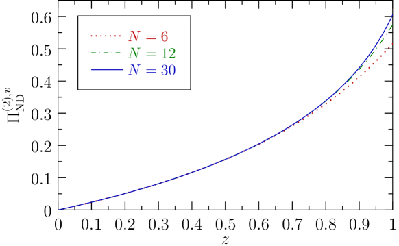
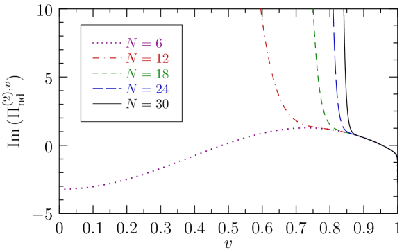
Figure 4: Convergence of the three-loop contribution to the low- and high-energy expansion of the non-diagonal vector correlator in the $\overline{\text{MS}}$ scheme for $n_{h}=1$, $n_{l}=3$. The upper figure shows the correlator in the low-energy range for different orders of the expansion in $z$. The lower figures show the behavior above threshold for both real and imaginary parts. Note that the high-energy expansion converges only above $v=0.8$ which corresponds to the three-particle cut.

In Fig. 4 we show the convergence of the series for the case of the non-diagonal vector correlator. The behavior of the series is shown both for the low-energy and the high-energy expansion. For the high-energy expansion we show the real and the imaginary part. Since the non-diagonal correlators have a cut through three heavy quark lines, the high-energy expansion converges only above $z=9$, which corresponds to a velocity of the heavy quark of $v=(z-1)/(z+1)=0.8$. This behavior can also clearly be observed in Tables 2 and 3 which show rapidly growing coefficients corresponding to a radius of convergence $r<1$. Since Table 4 contains only contributions from diagrams with a closed massless-quark loop, the coefficients are better behaved.

$n$	$\bar{C}^{(0),v}_{n}$	$\bar{C}^{(1),v}_{n}$	$\bar{C}^{(2),v}_{n}[1]$	$\bar{C}^{(2),v}_{n}[n_{h}]$	$\bar{C}^{(2),v}_{n}[n_{l}]$
$1$	$0.500000$	$0.457734$	$-1.51195$	$0.0166564$	$0.337837$
$2$	$0.133333$	$-0.0483080$	$-0.840974$	$-0.0369934$	$0.187255$
$3$	$0.0555556$	$-0.115602$	$-0.665554$	$-0.0289884$	$0.135615$
$4$	$0.0285714$	$-0.115219$	$-0.475376$	$-0.0213752$	$0.104474$
$5$	$0.0166667$	$-0.102152$	$-0.309702$	$-0.0161172$	$0.0832408$
$6$	$0.0105820$	$-0.0880811$	$-0.177592$	$-0.0125094$	$0.0679630$
$7$	$0.00714286$	$-0.0756354$	$-0.0753998$	$-0.00996452$	$0.0565728$
$8$	$0.00505051$	$-0.0651894$	$0.00291844$	$-0.00811379$	$0.0478459$
$9$	$0.00370370$	$-0.0565463$	$0.0628596$	$-0.00672995$	$0.0410083$
$10$	$0.00279720$	$-0.0494003$	$0.108797$	$-0.00566985$	$0.0355496$
$11$	$0.00216450$	$-0.0434648$	$0.144058$	$-0.00484063$	$0.0311210$
$12$	$0.00170940$	$-0.0385013$	$0.171144$	$-0.00418016$	$0.0274778$
$13$	$0.00137363$	$-0.0343196$	$0.191926$	$-0.00364579$	$0.0244440$
$14$	$0.00112045$	$-0.0307699$	$0.207816$	$-0.00320745$	$0.0218902$
$15$	$0.000925926$	$-0.0277347$	$0.219882$	$-0.00284350$	$0.0197199$
$16$	$0.000773994$	$-0.0251214$	$0.228940$	$-0.00253805$	$0.0178596$
$17$	$0.000653595$	$-0.0228568$	$0.235620$	$-0.00227923$	$0.0162527$
$18$	$0.000556948$	$-0.0208824$	$0.240408$	$-0.00205802$	$0.0148551$
$19$	$0.000478469$	$-0.0191512$	$0.243686$	$-0.00186749$	$0.0136316$
$20$	$0.000414079$	$-0.0176253$	$0.245754$	$-0.00170221$	$0.0125545$
$21$	$0.000360750$	$-0.0162738$	$0.246850$	$-0.00155793$	$0.0116011$
$22$	$0.000316206$	$-0.0150713$	$0.247164$	$-0.00143123$	$0.0107532$
$23$	$0.000278707$	$-0.0139968$	$0.246847$	$-0.00131937$	$0.00999562$
$24$	$0.000246914$	$-0.0130328$	$0.246023$	$-0.00122012$	$0.00931596$
$25$	$0.000219780$	$-0.0121648$	$0.244790$	$-0.00113166$	$0.00870382$
$26$	$0.000196483$	$-0.0113806$	$0.243229$	$-0.00105247$	$0.00815053$
$27$	$0.000176367$	$-0.0106696$	$0.241406$	$-0.000981314$	$0.00764873$
$28$	$0.000158907$	$-0.0100231$	$0.239376$	$-0.000917133$	$0.00719220$
$29$	$0.000143678$	$-0.00943357$	$0.237182$	$-0.000859046$	$0.00677564$
$30$	$0.000130336$	$-0.00889448$	$0.234861$	$-0.000806306$	$0.00639448$

Table 1: Numerical results for the low-energy moments for the non-diagonal vector correlator in the $\overline{\text{MS}}$ scheme.

$n$	$\bar{D}^{(2),v}_{n,0}[1]$	$\bar{D}^{(2),v}_{n,1}[1]$	$\bar{D}^{(2),v}_{n,2}[1]$	$\bar{D}^{(2),v}_{n,3}[1]$
$0$	$1.78284$	$-2.64761$	$1.83333$	$0$
$1$	$-17.7072$	$25.1337$	$-16.3333$	$3.16667$
$2$	$-60.1359$	$47.0000$	$-8.00000$	$0$
$3$	$-41.3176$	$-15.4431$	$16.0772$	$-3.32442$
$4$	$4.27239$	$-20.8764$	$5.72599$	$0.659122$
$5$	$7.18683$	$-11.8251$	$0.822323$	$-0.129739$
$6$	$0.493132$	$-5.22086$	$2.92024$	$-0.566886$
$7$	$-16.8712$	$-10.5240$	$9.71602$	$-0.991008$
$8$	$-56.8660$	$-43.6415$	$29.4833$	$-1.70280$
$9$	$-164.387$	$-190.388$	$94.9042$	$-2.87364$
$10$	$-485.549$	$-831.419$	$339.294$	$-4.95108$
$11$	$-1537.17$	$-3780.76$	$1357.43$	$-8.63056$
$12$	$-5240.01$	$-18141.8$	$6001.46$	$-15.2756$
$13$	$-18953.8$	$-91894.0$	$28790.4$	$-27.3450$
$14$	$-70903.6$	$-488762$	$147374$	$-49.4690$
$15$	$-264436$	$-2.71202\cdot 10^{6}$	$794591$	$-90.2629$
$16$	$-922552$	$-1.56052\cdot 10^{7}$	$4.46970\cdot 10^{6}$	$-165.935$
$17$	$-2.52510\cdot 10^{6}$	$-9.26482\cdot 10^{7}$	$2.60485\cdot 10^{7}$	$-306.988$
$18$	$-142055$	$-5.65199\cdot 10^{8}$	$1.56448\cdot 10^{8}$	$-571.093$
$19$	$8.11996\cdot 10^{7}$	$-3.53100\cdot 10^{9}$	$9.64408\cdot 10^{8}$	$-1067.52$
$20$	$9.74537\cdot 10^{8}$	$-2.25279\cdot 10^{10}$	$6.08196\cdot 10^{9}$	$-2003.91$
$21$	$8.94750\cdot 10^{9}$	$-1.46443\cdot 10^{11}$	$3.91351\cdot 10^{10}$	$-3775.71$
$22$	$7.44796\cdot 10^{10}$	$-9.68039\cdot 10^{11}$	$2.56374\cdot 10^{11}$	$-7137.78$
$23$	$5.91860\cdot 10^{11}$	$-6.49650\cdot 10^{12}$	$1.70673\cdot 10^{12}$	$-13533.8$
$24$	$4.59022\cdot 10^{12}$	$-4.41990\cdot 10^{13}$	$1.15282\cdot 10^{13}$	$-25729.9$
$25$	$3.51344\cdot 10^{13}$	$-3.04480\cdot 10^{14}$	$7.88989\cdot 10^{13}$	$-49035.5$
$26$	$2.67074\cdot 10^{14}$	$-2.12156\cdot 10^{15}$	$5.46505\cdot 10^{14}$	$-93657.0$
$27$	$2.02372\cdot 10^{15}$	$-1.49382\cdot 10^{16}$	$3.82727\cdot 10^{15}$	$-179244$
$28$	$1.53213\cdot 10^{16}$	$-1.06201\cdot 10^{17}$	$2.70750\cdot 10^{16}$	$-343676$
$29$	$1.16067\cdot 10^{17}$	$-7.61776\cdot 10^{17}$	$1.93326\cdot 10^{17}$	$-660072$
$30$	$8.80664\cdot 10^{17}$	$-5.50954\cdot 10^{18}$	$1.39237\cdot 10^{18}$	$-1.26974\cdot 10^{6}$

Table 2: Three-loop coefficients of the high-energy expansion for the non-diagonal vector correlator in the $\overline{\text{MS}}$ scheme with $n_{h}=n_{l}=0$.

$n$	$\bar{D}^{(2),v}_{n,0}[n_{h}]$	$\bar{D}^{(2),v}_{n,1}[n_{h}]$	$\bar{D}^{(2),v}_{n,2}[n_{h}]$	$\bar{D}^{(2),v}_{n,3}[n_{h}]$
$0$	$-0.251201$	$0.153727$	$-0.111111$	$0$
$1$	$0.154182$	$-1.14726$	$0.555556$	$-0.111111$
$2$	$3.61746$	$-1.14459$	$-0.666667$	$0$
$3$	$1.27971$	$2.67597$	$1.06790$	$0.185185$
$4$	$-3.99022$	$-1.81636$	$-0.861111$	$-0.543210$
$5$	$-8.59452$	$0.842895$	$1.23685$	$-1.15062$
$6$	$-25.2903$	$-2.26222$	$8.70815$	$-1.68560$
$7$	$-65.3844$	$-31.4942$	$28.2131$	$-2.18624$
$8$	$-164.223$	$-160.905$	$86.7525$	$-2.66878$
$9$	$-441.129$	$-715.641$	$295.743$	$-3.14070$
$10$	$-1320.45$	$-3233.48$	$1154.83$	$-3.60588$
$11$	$-4384.76$	$-15440.6$	$5072.08$	$-4.06652$
$12$	$-15690.9$	$-78173.7$	$24362.3$	$-4.52396$
$13$	$-58311.1$	$-416730$	$125176$	$-4.97906$
$14$	$-215239$	$-2.32045\cdot 10^{6}$	$677824$	$-5.43239$
$15$	$-732644$	$-1.34050\cdot 10^{7}$	$3.82947\cdot 10^{6}$	$-5.88438$
$16$	$-1.83932\cdot 10^{6}$	$-7.99084\cdot 10^{7}$	$2.24126\cdot 10^{7}$	$-6.33529$
$17$	$1.84847\cdot 10^{6}$	$-4.89431\cdot 10^{8}$	$1.35168\cdot 10^{8}$	$-6.78534$
$18$	$8.23216\cdot 10^{7}$	$-3.06952\cdot 10^{9}$	$8.36569\cdot 10^{8}$	$-7.23470$
$19$	$9.21471\cdot 10^{8}$	$-1.96567\cdot 10^{10}$	$5.29604\cdot 10^{9}$	$-7.68348$
$20$	$8.27344\cdot 10^{9}$	$-1.28233\cdot 10^{11}$	$3.42033\cdot 10^{10}$	$-8.13178$
$21$	$6.81847\cdot 10^{10}$	$-8.50550\cdot 10^{11}$	$2.24852\cdot 10^{11}$	$-8.57968$
$22$	$5.39132\cdot 10^{11}$	$-5.72647\cdot 10^{12}$	$1.50188\cdot 10^{12}$	$-9.02723$
$23$	$4.17068\cdot 10^{12}$	$-3.90796\cdot 10^{13}$	$1.01766\cdot 10^{13}$	$-9.47449$
$24$	$3.18860\cdot 10^{13}$	$-2.69998\cdot 10^{14}$	$6.98579\cdot 10^{13}$	$-9.92149$
$25$	$2.42300\cdot 10^{14}$	$-1.88650\cdot 10^{15}$	$4.85260\cdot 10^{14}$	$-10.3683$
$26$	$1.83633\cdot 10^{15}$	$-1.33179\cdot 10^{16}$	$3.40755\cdot 10^{15}$	$-10.8149$
$27$	$1.39098\cdot 10^{16}$	$-9.49177\cdot 10^{16}$	$2.41677\cdot 10^{16}$	$-11.2613$
$28$	$1.05453\cdot 10^{17}$	$-6.82454\cdot 10^{17}$	$1.72987\cdot 10^{17}$	$-11.7075$
$29$	$8.00841\cdot 10^{17}$	$-4.94695\cdot 10^{18}$	$1.24877\cdot 10^{18}$	$-12.1537$
$30$	$6.09583\cdot 10^{18}$	$-3.61318\cdot 10^{19}$	$9.08598\cdot 10^{18}$	$-12.5997$

Table 3: Three-loop contribution proportional to $n_{h}$ to the coefficients of the high-energy expansion for the non-diagonal vector correlator in the $\overline{\text{MS}}$ scheme.

$n$	$\bar{D}^{(2),v}_{n,0}[n_{l}]$	$\bar{D}^{(2),v}_{n,1}[n_{l}]$	$\bar{D}^{(2),v}_{n,2}[n_{l}]$	$\bar{D}^{(2),v}_{n,3}[n_{l}]$
$0$	$-0.730175$	$0.153727$	$-0.111111$	$0$
$1$	$-0.314922$	$-1.14726$	$0.555556$	$-0.111111$
$2$	$0.984271$	$-1.77778$	$0$	$0$
$3$	$1.27530$	$-0.0592818$	$-0.615226$	$0.0534979$
$4$	$0.544450$	$0.835905$	$-0.0709877$	$-0.0246914$
$5$	$0.0510031$	$0.410862$	$0.0306790$	$-0.00740741$
$6$	$-0.0437552$	$0.209240$	$0.0303704$	$-0.00329218$
$7$	$-0.0561161$	$0.117605$	$0.0233371$	$-0.00176367$
$8$	$-0.0503344$	$0.0722787$	$0.0177016$	$-0.00105820$
$9$	$-0.0420848$	$0.0475365$	$0.0136697$	$-0.000685871$
$10$	$-0.0347091$	$0.0329283$	$0.0107911$	$-0.000470312$
$11$	$-0.0287111$	$0.0237565$	$0.00869670$	$-0.000336700$
$12$	$-0.0239493$	$0.0177088$	$0.00713792$	$-0.000249408$
$13$	$-0.0201760$	$0.0135592$	$0.00595223$	$-0.000189934$
$14$	$-0.0171671$	$0.0106166$	$0.00503229$	$-0.000148000$
$15$	$-0.0147456$	$0.00847129$	$0.00430581$	$-0.000117578$
$16$	$-0.0127769$	$0.00687002$	$0.00372304$	$-0.0000949668$
$17$	$-0.0111601$	$0.00565028$	$0.00324902$	$-0.0000778089$
$18$	$-0.00981938$	$0.00470458$	$0.00285863$	$-0.0000645526$
$19$	$-0.00869741$	$0.00395987$	$0.00253355$	$-0.0000541477$
$20$	$-0.00775052$	$0.00336532$	$0.00226014$	$-0.0000458663$
$21$	$-0.00694509$	$0.00288479$	$0.00202813$	$-0.0000391926$
$22$	$-0.00625501$	$0.00249212$	$0.00182965$	$-0.0000337544$
$23$	$-0.00565976$	$0.00216805$	$0.00165859$	$-0.0000292783$
$24$	$-0.00514313$	$0.00189817$	$0.00151016$	$-0.0000255604$
$25$	$-0.00469214$	$0.00167159$	$0.00138059$	$-0.0000224467$
$26$	$-0.00429635$	$0.00147992$	$0.00126683$	$-0.0000198192$
$27$	$-0.00394727$	$0.00131666$	$0.00116643$	$-0.0000175864$
$28$	$-0.00363797$	$0.00117672$	$0.00107740$	$-0.0000156771$
$29$	$-0.00336274$	$0.00105607$	$0.000998082$	$-0.0000140345$
$30$	$-0.00311683$	$0.000951473$	$0.000927135$	$-0.0000126137$

Table 4: Three-loop contribution proportional to $n_{l}$ to the coefficients of the high-energy expansion for the non-diagonal vector correlator in the $\overline{\text{MS}}$ scheme.

4 Conclusion

We have used modern techniques to compute 30 terms in the low-energy expansion of the non-diagonal scalar and vector correlators, matching the already available information on diagonal correlators [21]. Using slightly modified methods we have also obtained 30 coefficients in the high-energy expansion of both non-diagonal and diagonal correlators. Due to multiply massive cuts in some of the contributing diagrams it is expected that the high-energy expansion already breaks down significantly above the physical threshold. Using only the previously available coefficients this behaviour is rather difficult to see. The newly computed coefficients, however, clearly support the presence of such a divergence.

As a final remark it should be noted that the expansion via differential equations used in this publication is rather efficient. This means that it is easy to obtain significantly more terms in the expansions if the need arises.

References

- [1] M. A. Shifman, A. I. Vainshtein, V. I. Zakharov. Nucl. Phys., B147:385–447, 1979.
- [2] V. A. Novikov, et al. Phys. Rept., 41:1–133, 1978.
- [3] J. H. Kühn, M. Steinhauser. Nucl. Phys., B619:588–602, 2001.
- [4] R. Boughezal, M. Czakon, T. Schutzmeier. Phys. Rev., D74:074006, 2006.
- [5] J. H. Kühn, M. Steinhauser, C. Sturm. Nucl. Phys., B778:192–215, 2007.
- [6] K. G. Chetyrkin, J. H. Kühn, A. Maier, P. Maierhöfer, P. Marquard, M. Steinhauser, C. Sturm. Phys. Rev., D80:074010, 2009.
- [7] K. Chetyrkin, J. Kühn, A. Maier, P. Maierhofer, P. Marquard, et al. 2010. arXiv:1010.6157.
- [8] B. Dehnadi, A. H. Hoang, V. Mateu, S. Zebarjad. 2011. arXiv:1102.2264.
- [9] S. Bodenstein, J. Bordes, C. Dominguez, J. Penarrocha, K. Schilcher. Phys.Rev., D82:114013, 2010.
- [10] I. Allison, et al. Phys. Rev., D78:054513, 2008.
- [11] C. McNeile, C. T. H. Davies, E. Follana, K. Hornbostel, G. P. Lepage. Phys.Rev., D82:034512, 2010.
- [12] A. A. Penin, M. Steinhauser. Phys. Rev., D65:054006, 2002.
- [13] W. Lucha, D. Melikhov, S. Simula. J.Phys.G, G38:105002, 2011.
- [14] P. A. Baikov, K. G. Chetyrkin, J. H. Kühn. Phys. Rev. Lett., 101:012002, 2008.
- [15] M. Davier, S. Descotes-Genon, A. Höcker, B. Malaescu, Z. Zhang. Eur.Phys.J., C56:305–322, 2008.
- [16] A. O. G. Källén, A. Sabry. Kong. Dan. Vid. Sel. Mat. Fys. Med., 29N17:1–20, 1955.
- [17] L. Reinders, S. Yazaki, H. Rubinstein. Phys.Lett., B103:63, 1981.
- [18] K. G. Chetyrkin, J. H. Kühn, M. Steinhauser. Nucl. Phys., B505:40–64, 1997.
- [19] K. G. Chetyrkin, M. Steinhauser. Eur. Phys. J., C21:319–338, 2001.
- [20] R. Boughezal, M. Czakon, T. Schutzmeier. Nucl. Phys. Proc. Suppl., 160:160–164, 2006.
- [21] A. Maier, P. Maierhöfer, P. Marquard. Nucl. Phys., B797:218–242, 2008.
- [22] K. G. Chetyrkin, J. H. Kühn, C. Sturm. Eur. Phys. J., C48:107–110, 2006.
- [23] C. Sturm. JHEP, 09:075, 2008.
- [24] A. Maier, P. Maierhöfer, P. Marquard. Phys. Lett., B669:88–91, 2008.
- [25] A. Maier, P. Maierhöfer, P. Marquard, A. V. Smirnov. Nucl. Phys., B824:1–18, 2010.
- [26] P. A. Baikov, K. G. Chetyrkin, J. H. Kühn. 2009. arXiv:0906.2987.
- [27] J. Hoff, M. Steinhauser. Nucl.Phys., B849:610–627, 2011.
- [28] K. G. Chetyrkin, J. H. Kühn, M. Steinhauser. Nucl. Phys., B482:213–240, 1996.
- [29] Y. Kiyo, A. Maier, P. Maierhöfer, P. Marquard. Nucl. Phys., B823:269–287, 2009.
- [30] A. H. Hoang, V. Mateu, S. Mohammad Zebarjad. Nucl. Phys., B813:349–369, 2009.
- [31] D. Greynat, S. Peris. Phys.Rev., D82:034030, 2010.
- [32] D. Greynat, P. Masjuan, S. Peris. 2011. arXiv:1104.3425.
- [33] P. Nogueira. J.Comput.Phys., 105:279–289, 1993.
- [34] R. Harlander, T. Seidensticker, M. Steinhauser Phys. Lett., B426:125, 1998; T. Seidensticker arXiv:hep-ph/9905298.
- [35] K. G. Chetyrkin, F. V. Tkachov. Nucl. Phys., B192:159–204, 1981.
- [36] S. Laporta. Int.J.Mod.Phys., A15:5087–5159, 2000.
- [37] P. Marquard, D. Seidel. Unpublished.
- [38] J. Vermaseren. 2000. arXiv:math-ph/0010025.
- [39] A. Kotikov. Phys.Lett., B254:158–164, 1991.
- [40] E. Remiddi. Nuovo Cim., A110:1435–1452, 1997.
- [41] M. Caffo, H. Czyz, S. Laporta, E. Remiddi. Nuovo Cim., A111:365–389, 1998.
- [42] S. Larin. Phys.Lett., B303:113–118, 1993.