The Renormalization Effects in the Microstrip-SQUID Amplifier

Abstract

The peculiarities of the microstrip-DC SQUID amplifier caused by the resonant structure of the input circuit are analyzed. It is shown that the mutual inductance, that couples the input circuit and the SQUID loop, depends on the frequency of electromagnetic field. The renormalization of the SQUID parameters due to the screening effect of the input circuit vanishes when the Josephson frequency is much greater than the signal frequency.

LA-UR 11-06109

1 Introduction

For a long time, the SQUID has been used as the most sensitive detector of a magnetic flux. Recently, there has been growing interest in the development of a low noise radio-frequency and microwave amplifiers, for example, for axion detection [1, 2] or for the measurement of superconducting quantum bits [3, 4]. For these applications, the SQUID is a leading candidate due to its low power dissipation and excellent noise properties.

In typical SQUID amplifiers, the input signal is injected into an input coil that is coupled to the SQUID washer. The input coil is deposited on top of a dielectric layer, which covers the washer. The coupling of the input circuit to the SQUID can significantly modify the properties of both the SQUID and the input coil. A modification of the SQUID by a coupled inductance was pointed out by Zimmerman [5] and studied by Clarke and coworkers [6]-[8]. The most important influence of the input coil on the SQUID is the reduction of the loop inductance. The macroscopic parameters of the SQUID take the renormalized values corresponding to the reduced loop inductance.

Martinis and Clarke [6] have pointed out that the renormalization effect, due to the mutual inductance of input circuit and SQUID, can be suppressed by parasitic capacitances between the input coil and the washer. Parasitic capacitances, being widely distributed, cause the gain to fall at high frequencies. More recently, the idea of using the capacitance between the coil and the washer to form a resonant microstrip has arisen [9] and developed [10]. The deleterious effect of the parasitic capacitance was addressed by operating the input coil as a transmission line resonator. In this case, the input signal was applied between one end of the coil and the washer, while the other end of the coil was left open.

The transmission line resonator has an infinite set of eigenfrequencies that is in contrast to a resonator with lumped capacitance and inductance. In our model, for each eigenfrequency, $\omega_{n}$, we will put in correspondence a couple of values of $C_{n}$ and $L_{n}$, which satisfy the relation, $\omega_{n}=\big{(}L_{n}C_{n}\big{)}^{-1/2}$. The input circuit response to the SQUID signals depends on the characteristic frequencies of the circuit. The Josephson frequency, $\omega_{J}$, and the frequency of the input signal, $\omega$, are the most important ones. Usually, the amplifier operates in the low frequency regime of $\omega_{J}>>\omega$. Therefore, one can expect that the response of the input circuit to the high-frequency SQUID signal will differ significantly from the low-frequency response. The physical picture is very similar to the effect of parasitic capacitances on SQUID amplification.

2 Transmission-line modes

A non-dissipative lumped-element resonator with the inductance, $L_{lump}$, and capacitance, $C_{lump}$, can be described by the oscillator Hamiltonian,

$$H=\frac{p^{2}}{2L_{lump}}+\frac{q^{2}}{2C_{lump}},$$ (1)

where $L_{lump}$ and $(C_{lump})^{-1}$ are the effective mass and the spring constant of the oscillator, and $p$ and $q$ are the corresponding momentum and coordinate. The oscillator frequency is: $\omega_{r}=(L_{lump}C_{lump})^{-1/2}$.

The superconducting transmission line is characterized by infinite number of oscillators. Its Hamiltonian is [11, 12]:

$$H=\sum_{n}\frac{1}{2}\bigg{(}\frac{\pi^{2}_{n}}{l}+\frac{\varphi^{2}_{n}}{c}k_{n}^{2}\bigg{)},$$ (2)

where $\pi_{n}$ and $\varphi_{n}$ are the canonically conjugated “momentum” and “coordinate”, $l$ and $c$ are the inductance and the capacitance per unit length, respectively. In the case of open ends of the line, the value of $k_{n}$ is equal to $\pi n/\Lambda$, where $n=1,2,3,...$, and $\Lambda$ is the length of the line. It follows from Eq. (2) that the frequency of the $n$th oscillator is,

$$\omega_{n}=k_{n}(lc)^{-1/2}.$$ (3)

For each resonator mode, $n$, the current and the voltage profiles on the resonator are given by sinusoidal and cosinusoidal distributions, respectively,

$$I_{n}\sim\sin(n\pi x/\Lambda),\quad\;V_{n}\sim\cos(n\pi x/\Lambda),$$ (4)

where the beginning of the line is at $x=0$.

After changing the variables,

$$\pi_{n}^{\prime}=\pi_{n}/{\sqrt{k_{n}}}~{},\quad\,\varphi_{n}^{\prime}=\varphi_{n}{\sqrt{k_{n}}}~{},$$

Eq. (2) can be rewritten as:

$$H=\sum_{n}\frac{1}{2}\bigg{(}\frac{\pi^{\prime 2}_{n}}{l/k_{n}}+\frac{\varphi^{\prime 2}_{n}}{c/k_{n}}\bigg{)}.$$ (5)

The quantities, $l/k_{n}$ and $\>c/k_{n}$, have the dimensions of the inductance and capacitance, respectively. Comparing each summand in Eq. (5) with Eq. (1), we conclude that the quantities, $L_{n}\equiv l/k_{n}$ and $C_{n}\equiv c/k_{n}$, are the inductance and the capacitance of the $n$th resonator. The value, $(L_{n}C_{n})^{-1/2}$, coincides with the frequency, $\omega_{n}$, given by Eq. (3).

It follows that the values, $L_{n}$ and $C_{n}$, depend on the number $n$ as $1/n$. Hence, $L_{n}=L_{1}/n,\>C_{n}=C_{1}/n$. For the case of the fundamental frequency ($n=1$), we have:

$$L_{1}={{\Lambda}\over{\pi}}l,~{}C_{1}={{\Lambda}\over{\pi}}c.$$ (6)

A set of resonances in the transmission line can modify the renormalization of the SQUID parameters. In what follows we analyze this phenomenon in more details.

3 Scheme of the microstrip-SQUID amplifier

Fig. 1 shows schematically the equivalent circuit of the microstrip-SQUID amplifier. $V_{i}$ is the amplitude of the input voltage; $R_{i}$ and $R$ are the resistances of the voltage source and the resistance shunting the stripline, respectively; $C_{i}$ is the coupling capacitance.

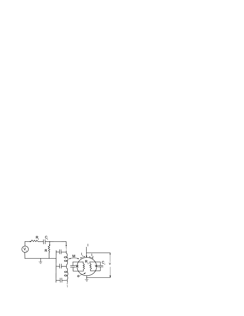
Figure 1: The equivalent circuit of the microstrip-SQUID amplifier. The resonant microstrip is shown as a sequence of lumped inductances and capacitances. The mutual inductance, $M$, couples the input circuit to the SQUID loop whose inductance is, $L_{J}$.

The two Josephson junctions are in parallel with the resistances, $R_{J}$ (which can be external shunts) and capacitances, $C_{J}$. The shunting effect of these elements provides nonhysteretic characteristics for the SQUID. The Josephson junctions are connected in parallel, thus forming a superconducting loop of inductance, $L_{J}$. The transmission line is coupled to the SQUID loop by the mutual inductance, $M$. An external dc current bias, $I$, and a dc flux, $\Phi$, are applied to provide the most favorable values of the transfer function, ${dV}/{d\Phi}\equiv V_{\Phi}$ , where $\Phi$ is the magnetic flux inside the loop. Here we will not take into account the noise component of the electromagnetic fields which is present in the circuit due to the resistances, $R_{J},\>R,\>R_{i}$, and generated by external sources.

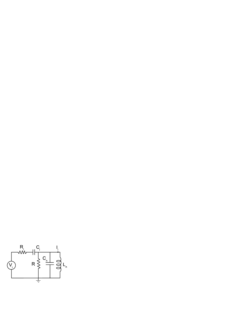
Figure 2: Lumped element model of the input circuit. In the vicinity of the $n$th resonance ($\omega\approx\omega_{n}$) the transmission line is represented by the capacitance, $C_{n}$, and the inductance, $L_{n}$.

The transmission line current caused by the input voltage, $V_{i}$, depends on the frequency, $\omega$. In the vicinity of some eigenfrequency, $\omega_{n}$, the input circuit can be described by the equivalent scheme shown in Fig. 2. Usually $\omega$ is close to the fundamental frequency, $\omega_{1}$. For this particular case and in the absence of the SQUID, the forward impedance of the input circuit, defined as $Z={V_{i}}/{I_{i}}_{|M=0}$, is:

$$Z=\frac{L_{1}}{C_{i}}\bigg{\{}i\bigg{[}\omega\bigg{(}C_{1}+C_{i}+C_{i}\frac{R_{i}}{R}\bigg{)}-\frac{1}{\omega L_{1}}\bigg{]}+\frac{1}{R}-R_{i}C_{i}\bigg{(}\omega^{2}C_{1}-\frac{1}{L_{1}}\bigg{)}\bigg{\}}.$$ (7)

As we see, the resonant properties of the input circuit depend not only on the parameters of the microstrip but also on the presence of other elements. (The effect of coupling capacitance on amplification was studied experimentally in [13].) Also, the SQUID parameters affect the input circuit characteristics via the mutual inductance, $M$.

Similar to $L_{n}$ and $C_{n}$, the value of $M$ depends on the frequency of radiation. The following can help to determine this dependence. It can be seen from Eq. (4), that the current of the $n$th mode changes its direction at $x=\Lambda m/n$, where $m$ is an integer ($m<n$). The total flux generated by the $n$th mode in the SQUID loop is smaller than it could be in the case of a constant sign (for example, in the case of $n=1$). It is reasonable to approximate $M(\omega_{n})$ by

$$M(\omega_{n})\equiv M_{n}=M_{1}/n.$$ (8)

The coefficient $1/n$ accounts for the reduction of the high-frequency flux, generated in the loop. Eq.(8) is a good approximation for a signal frequency, $\omega\approx\omega_{1}$, as well as for the Josephson frequency, $\omega>>\omega_{1}$. In what follows, both characteristic frequencies are of our major interest.

For high frequencies, where discreteness of the transmission line spectrum is not important, we can consider

$$M(\omega)\approx M_{1}\frac{\omega_{1}}{\omega}.$$ (9)

The theoretical analysis of amplification should account for the dependence of $M$ on the frequency of electromagnetic field.

4 Equations of motion for the coupled microstrip-SQUID

In this Section, we analyze how the frequency dependence of $M$, given by Eq. (9), modifies the renormalization effect of the SQUID parameters. We will see that the renormalization vanishes if the Josephson frequency is much larger than the input signal frequency.

The standard system of equations describing the dynamics of the SQUID is given by:

$$J=\frac{1}{2}(I_{2}-I_{1}),$$

$$I=I_{1}+I_{2},$$

$$V=\frac{\Phi_{0}}{4\pi}\bigg{(}\dot{\delta}_{1}+\dot{\delta}_{2}\bigg{)},$$

$$\Phi+L_{J}J+\widetilde{MI_{i}}=\frac{\Phi_{0}}{2\pi}\bigg{(}\delta_{1}-\delta_{2}\bigg{)},$$

$$\frac{\Phi_{0}}{2\pi}C_{J}\ddot{\delta}_{1}+\frac{\Phi_{0}}{2\pi R_{J}}\dot{\delta}_{1}=I_{1}-I_{c}\sin\delta_{1},$$

$$\frac{\Phi_{0}}{2\pi}C_{J}\ddot{\delta}_{2}+\frac{\Phi_{0}}{2\pi R_{J}}\dot{\delta}_{2}=I_{2}-I_{c}\sin\delta_{2},$$ (10)

where, $\delta_{1,2}$, is the phase difference across the left or right junction, respectively, $\Phi_{0}=\frac{h}{2e}$ is the flux quantum, $e$ is the electron charge ($e>0$ here), $I_{c}$ is the critical value of the Josephson current through an individual junction. A wide tilde, ($\widetilde{...}$), indicates the convolution:

$$\widetilde{MI_{i}}=\int_{-\infty}^{t}dt^{\prime}M(t-t^{\prime})I_{i}(t^{\prime}),$$ (11)

where the mutual inductance, $M(t)$, ($M(t)=0$ for $t<0$) can be expressed via its Fourier-transform as,

$$M(t)=\frac{1}{2\pi}\int_{-\infty}^{+\infty}d\omega e^{i\omega t}M(\omega).$$

The fourth equation in (10) explicitly describes the SQUID-input circuit coupling via the mutual inductance, $M$. This coupling arises from the current, $I_{i}$, which induces a magnetic flux in the SQUID loop, thus changing the voltage, $V$, across the SQUID.

On the other hand, the current around the loop, $J$, induces a voltage, $-\partial_{t}\widetilde{MJ}$, in the transmission line of the input circuit. Hence, the current, $I_{i}$, is generated by both the external voltage, $V_{i}$, and the voltage caused by the circulating current, $J$. In the frequency domain, $I_{i}$ is given by:

$$I_{i}(\omega^{\prime})=\frac{V_{i}(\omega^{\prime})}{Z_{\omega^{\prime}}}-i\frac{\omega^{\prime}M(\omega^{\prime})J(\omega^{\prime})}{Z_{\omega^{\prime}}}\frac{C(\omega^{\prime})}{C_{i}},$$ (12)

where the input voltage is considered to be a harmonic function, $V_{i}(t)=V_{i}e^{i\omega t}$, and $V_{i}(\omega^{\prime})=2\pi V_{i}\delta(\omega-\omega^{\prime})$. We have also assumed, for simplicity, that the resistance of the source and of the coupling capacitance are small: $R_{i}<<R,\>C_{i}<<C$.

The quantities, $L$ and $C$, depend on the frequency, $\omega^{\prime}$, similar to the dependence of $M(\omega^{\prime})$:

$$L(\omega^{\prime})\approx L_{1}\frac{\omega_{1}}{\omega^{\prime}},\>\,C(\omega^{\prime})\approx C_{1}\frac{\omega_{1}}{\omega^{\prime}}.$$ (13)

Substituting the expression (12) for $I_{i}$ into the fourth equation of the system (10), we have:

$$\Phi+L_{J}J+\frac{M_{1}V_{i}(t)}{Z(\omega)}-$$

$$\int_{-\infty}^{t}dt^{\prime}M(t-t^{\prime})\int_{-\infty}^{+\infty}\frac{d\omega^{\prime}}{2\pi}i\omega^{\prime}e^{i\omega^{\prime}t^{\prime}}\frac{M_{\omega^{\prime}}J_{\omega^{\prime}}C_{\omega^{\prime}}}{Z(\omega^{\prime})C_{i}}=\frac{\Phi_{0}}{2\pi}\bigg{(}\delta_{1}-\delta_{2}\bigg{)}.$$ (14)

The third term in the left-hand side of Eq. (14) describes the low-frequency (the input voltage frequency) contribution to the flux threading the SQUID loop. The fourth term represents both the low-frequency and the high-frequency components. The high frequency is in the range close to $\omega_{J}$. It follows from the analysis of Section 3 (see Eq. (9)) that,

$$M^{2}(\omega_{J})\approx M_{1}^{2}\frac{\omega_{1}^{2}}{\omega_{J}^{2}}<<M_{1}^{2}.$$ (15)

Eq. (15) shows that the high-frequency contribution to the total flux arising from strip-line-SQUID coupling can be neglected. In this case, Eq. (14) reduces to

$$\Phi+L_{J}J+\Delta\Phi(t)=\frac{\Phi_{0}}{2\pi}\bigg{(}\delta_{1}-\delta_{2}\bigg{)},$$ (16)

where $\Delta\Phi(t)$ contains only the low-frequency Fourier-components:

$$\Delta\Phi(\omega^{\prime})=\frac{M_{1}V_{i}(\omega^{\prime})}{Z(\omega^{\prime})}-\frac{C_{1}M_{1}^{2}}{C_{i}}i\omega^{\prime}\frac{J_{\omega^{\prime}}}{Z(\omega^{\prime})}.$$ (17)

The frequency, $\omega^{\prime}$, in Eq. (17) is in the vicinity of the input voltage frequency $\omega$ ($|\omega^{\prime}-\omega|<<\omega)$.

Following the arguments of Ref. [6], we assume that the low-frequency components, $J(\omega)$ and $V(\omega)$, are generated by a small input voltage, $V_{i}$. By this reason, we consider both of them to be small quantities also. Considering a solution of the unperturbed SQUID equations to be known, we can express the linear response to the “external” flux, $\Delta\Phi$, as

$$V(t)=V_{\Phi}\Delta\Phi(t),\;\;J(t)=J_{\Phi}\Delta\Phi(t),$$ (18)

where $V_{\Phi}\equiv\partial V/\partial\Phi$ and $J_{\Phi}\equiv\partial J/\partial\Phi$. In contrast to the main result of the Reference [6], the derivatives in Eq. (18) should be those of the bare SQUID circuit (with non-renormalized inductance, $L_{J}$). This means that the high-frequency screening of the input circuit is negligible.

Using Eqs. (16)-(18), we can easily obtain the microstrip amplifier gain. If we represent the output voltage as $V(t)=Ve^{i\omega t}$, then the gain is given by:

$$\frac{V}{V_{i}}=\frac{M_{1}V_{\Phi}}{Z_{\omega}+J_{\Phi}i\omega M_{1}^{2}C_{1}/C_{i}}.$$ (19)

The second term in the denominator of Eq. (19) describes the modification of the low-frequency input impedance. This modification is due to the SQUID back action. At the same time, the coefficients $V_{\Phi}$ and $J_{\Phi}$ are taken for a bare SQUID. This corresponds to the physical picture in which the effective coupling of both sub-systems through the mutual inductance occurs at the signal frequency. The coupling becomes weak at high (Josephson) frequency.

5 Conclusion

Using the transmission line as a resonator of the input circuit does not result in a renormalization of the SQUID parameters, if the Josephson frequency is much greater than the frequency of the input signal. A similar effect was analyzed in [6]. The authors have discussed the influence of parasitic capacitances between the turns of the input coil or between the input coil and the SQUID, on the amplifier dynamics. It was shown that there was no current flow at the Josephson frequency in the input circuit in the presence of large parasitic capacitances. In this case, the reduced SQUID parameters are replaced with the bare SQUID parameters.

The presence or absence of the renormalization effect is of great importance for optimization of the input circuit parameters and achieving desirable gains especially in the gigahertz frequency region. It is worth mentioning, that the maximum SQUID amplification is restricted by the value of $R_{J}/L_{J}$ [14]. The renormalized inductance of the loop is smaller than the bare inductance, $L_{J}$. This explains the tendency of gain decrease with the increase of the signal frequency that was observed experimentally (see, for example, Ref. [15]).

Summarizing, in the limit of very high Josephson frequencies, there is no difference what kind of capacitance is in the input circuit. In both cases (parasitic irregular capacitance or smoothly distributed capacitance of the transmission line), a similar shunting effect causes the reflection of the SQUID signal by the input circuit. This prevents a renormalization of the SQUID parameters.

6 Acknowledgment

We thank D. Kinion for useful discussions. This work was carried out under the auspices of the National Nuclear Security Administration of the U.S. Department of Energy at the Los Alamos National Laboratory under Contract No. DE-AC52- 06NA25396, and was funded by the Office of the Director of National Intelligence (ODNI), and Intelligence Advanced Research Projects Activity (IARPA). All statements of fact, opinion or conclusions contained herein are those of the authors and should not be construed as representing the official views or policies of IARPA, the ODNI, or the U.S. Government.

References

- [1] R. Bradley, J. Clarke, D. Kinion, L.J. Rosenberg, K. van Bibber, S. Matsuki, M. Muck, and P. Sikivie, Rev. Mod. Phys, 75, 777 (2003).
- [2] S.J. Asztalos et al, Phys. Rev. Lett. 104, 041301 (2010).
- [3] S. Michotte, Appl. Phys. Lett. 94, 122512 (2009).
- [4] I. Serban, B.L.T. Plourde, and F.K. Wilhelm, Phys. Rev. B 78, 054507 (2008).
- [5] J.E. Zimmerman, J. Appl. Phys. 42, 4483 (1971).
- [6] J.M. Martinis, J. Clarke, J. Low Temp. Phys. 61, 227 (1985)
- [7] C. Hilbert, J. Clarke, J. Low Temp. Phys., 61, 237 (1985).
- [8] C. Hilbert, J. Clarke, J. Low Temp. Phys., 61, 263 (1985).
- [9] M. Muck, M O. Andre, J. Clarke, J. Gail, and Ch. Heiden, Appl. Phys. Lett. 72, 2885 (1998).
- [10] M. Muck, M O. Andre, J. Clarke, J. Gail, and Ch. Heiden, Nucl. Phys. B 72, 145 (1999).
- [11] A. Blais, R.S. Huang, A. Wallraff, S.M. Girvin, and R.J. Schoelkopf, Phys. Rev. A 69, 062320 (2004).
- [12] A.A. Clerk, M.H. Devoret, S.M. Girvin, F. Marquardt, R.J. Schoelkopf, http://arxiv.org/abs/0810.4729.
- [13] D. Kinion and J. Clarke, Appl. Phys. Lett. 92, 172503 (2008).
- [14] J. Clarke, A.T. Lee, M. Muck, and P.L. Richards, SQUID Voltmeters and Amplifiers, in The SQUID Handbook, Vol. II, Applications of SQUIDs and SQUID systems, (eds. John Clarke, Alex I. Braginski), Weinheim (2006), pp. 1-93.
- [15] M. Muck and R. McDermott, Supercond. Sci. Technol., 23, 093001 (2010).