Transitional dynamics of a phase qubit-resonator system: requirements for fast readout of a phase qubit

Abstract

We examine the non-stationary evolution of a coupled qubit-
transmission line-resonator system coupled to an external drive and the resonator environment. By solving the equation for a non-stationary resonator field, we determined the requirements for a single-shot non-destructive dispersive measurement of the phase qubit state. Reliable isolation of the qubit from the “electromagnetic environment” is necessary for a dispersive readout and can be achieved if the whole system interacts with the external fields only through the resonator that is weakly coupled to the qubit. A set of inequalities involving resonator-qubit detuning and coupling parameter, the resonator leakage and the measurement time, together with the requirement of multi-photon outgoing flux is derived. It is shown, in particular, that a decrease of the measurement time requires an increase of the resonator leakage. This increase results in reducing the quality factor and decreasing the resolution of the resonator eigenfrequencies corresponding to different qubit states. The consistent character of the derived inequalities for two sets of experimental parameters is discussed.

The obtained results will be useful for optimal design of experimental setups, parameters, and measurement protocols.

LA-UR-11-11790

1 Introduction

The measurement of qubits is an important step in quantum information processing. For accurate qubit detection, the readout has to be faster than the qubit relaxation time. Moreover, to implement quantum error correction, the readout time must be less than the decoherence time. The relaxation processes can be of different origin (even due to the qubit-vacuum interaction). Also, the effects of measuring devices on the behavior of qubit states during the readout time are of great importance [1]-[3].

The simplest scheme for fast qubit readout of the phase qubit, based on the tunneling effect, (single-shot measurement) has been implemented and studied in [4]-[8]. According to this scheme, the measurement pulse adiabatically reduces the barrier between the potential wells, one of which forms the qubit states. As a result, the qubit in the upper state switches by tunneling into the neighboring well with probability close to one, while the qubit in the lower state remains unchanged. This kind of readout is limited by the strong current noise back action from the measurement device on the qubit. Moreover, this demolition measurement process destroys the qubit states which is unacceptable for most applications.

The scheme of dispersive readout of qubit states has evident advantages. In what follows, we consider the case in which an external device probes the qubit state indirectly via a transmission line resonator (a two sided cavity) weakly coupled to the qubit. This scheme allows repeated measurements. The presence of the qubit-resonator coupling causes the resonator eigenfrequency to be dependent on the qubit state. Hence, the number of photons in the resonator, being dependent on the probe field-resonator detuning, depends on the qubit state. (This number is maximal for zero detuning.) For this reason, the field going out of the resonator contains information about the resonator state as well as about the qubit state.

The amplitude of the transmitted field depends on the photon number in the resonator and on the resonator leakage. The increase of both quantities results in an increase of the transmitted signal that in general improves the signal-to-noise ratio. However, both of these factors decrease the qubit relaxation time due to the qubit-resonator interaction. Moreover, resonators with high leakage (low quality factor) lose their ability to filter out those external noises which penetrate into the low-temperature region from the “external world”. Also, for a relatively large number of photons in the resonator, the qubit-resonator interaction cannot be considered to be weak, and the advantages of the dispersive measurement, based on the perturbation approach, disappear.

The optimal choice of both the readout strategy and the setup parameters can be facilitated by means of theoretical description of the physical processes involved in the course of readout. In what follows, we use our recent approach [9] which makes it possible to obtain explicit expressions for the photon numbers and the measurement-induced relaxation rate of the qubit. We derive a set of inequalities which are required to provide a single-shot dispersive measurement, and we present examples of the qubit and resonator parameters.

2 Hamiltonian and equations of motion

As in our previous paper [9], we consider a flux-biased phase qubit embedded in a symmetric transmission line by a set of distributed inductances and capacitances. This is shown schematically in Fig. 1. The qubit is coupled to the center of the transmission line by the capacitance, $C_{g}$, leading to their effective interaction strength, $g$. The qubit transition frequency, $\omega_{q}$, is tunable by varying an external flux, $\Phi$, shown schematically in Fig. 1. It is assumed that $\omega_{q}$ as well as the frequency of the external drive, $\omega_{d}$, is close to one of the eigenfrequencies of the transmission line, $\omega_{r}$. In this case, one can consider the transmission line as a resonator with a lumped inductance, $L_{r}$, and a capacitance, $C_{r}$. Then, the transmission line can be described in terms of a harmonic oscillator characterized by the single eigenfrequency, $\omega_{r}=(L_{r}C_{r})^{-1/2}$.

The total Hamiltonian is,

$$H=-{1\over 2}\hbar\omega_{q}\sigma_{z}+\hbar\omega_{r}\bigg{(}a^{\dagger}a+{1\over 2}\bigg{)}+\sum_{n}\hbar\omega_{n}\bigg{(}b^{\dagger}_{n}b_{n}+{1\over 2}\bigg{)}+$$

$$i\hbar g\sigma_{y}\bigg{(}a^{\dagger}-a\bigg{)}+i\hbar\sum_{n}f_{n}\bigg{(}b_{n}a^{\dagger}-b^{+}_{n}a\bigg{)}+i\hbar f_{0}\bigg{(}ca^{\dagger}-c^{\dagger}a\bigg{)},$$ (1)

where $\sigma_{z}$ is the Pauli operator, $a^{\dagger},b_{n}^{\dagger},c^{\dagger}(a,b_{n},c)$ are the creation (annihilation) operators of the resonator, bath, and drive excitations, respectively. The bath is modeled by an infinite set of harmonic oscillators. (See Refs. [10] and [11].)

The qubit-resonator interaction term (the fourth term in (1)) couples the variables of both subsystems. It is evident that only even harmonics of the transmission line are coupled with the qubit. We consider that the second harmonic has a frequency close to the qubit frequency. In the center of the transmission line, the voltage of the second harmonic is equal to [1],

$$V(t)=-\sqrt{\frac{\hbar\omega_{r}}{Lc}}\big{(}a+a^{+}\big{)},$$

where $L$ and $c$ are, correspondingly, the length of the line and its capacitance per unit length. For a given term for the voltage, $V(t)$, applied to both, $C_{g}$ and the qubit loop, we can easily express the interaction strength, $g$, as a function of other parameters of the system. This interaction strength, $g$, is given by the expression,

$$g=C_{g}\sqrt{\frac{\omega_{r}\omega_{q}}{2LcC_{J}}}.$$

For calculational simplicity, we approximated the potential energy of the qubit by a parabolic dependence on the effective coordinate. More details can be found in [12].

As one can see from Eq. 1, the interaction term is linear in the qubit and the resonator variables. Alternative interaction Hamiltonians (nonlinear in the resonator variables) describe the situation considered in [13] - [16].

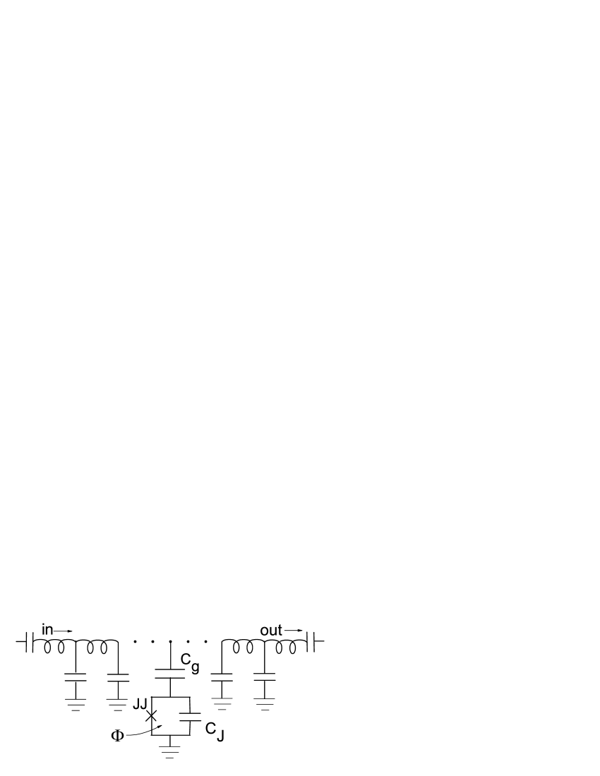
Figure 1: A scheme of the qubit-transmission-line system. $C_{J}$ is the capacitance shunting the Josephson junction, JJ. $C_{g}$ is the capacitance coupling the qubit and the transmission line. $\Phi$ is the external flux threading the qubit loop.

The resonator-thermostat and resonator-drive interaction terms are similar to the resonator-qubit interaction. The analytical approach in Ref. [9] is based on a set of inequalities,

$$|\omega_{ij}|<<\omega_{i},\omega_{j},\quad\omega_{ij}\equiv\omega_{i}-\omega_{j},$$ (2)

where the indices $i,j$ indicate the corresponding frequencies, $\omega_{q,r,d}$. The relations (2) indicate that all frequencies are close to each other.

Moreover, inequalities (2) were complemented by the requirement of a dispersive regime for our Hamiltonian. Usually, this is written in a form,

$$\frac{g}{|\omega_{qr}|}<<1.$$ (3)

Taking into account the fact that the interaction term depends linearly on $a$ and $a^{\dagger}$, a more accurate criterion can be written:

$$\frac{g\sqrt{\tilde{n}_{r}}}{|\omega_{qr}|}<<1,$$ (4)

where $\tilde{n}_{r}$ is the characteristic photon number in the resonator.

Considering all of the operators in the Heisenberg representation, we have derived in [9] the equation of motion for the resonator field, $a(t)$,

$$\bigg{[}\partial_{t}+i\bigg{(}\omega_{r}-\chi\sigma_{z}\bigg{)}+\frac{\kappa}{2}\bigg{]}a=f_{0}c+\sum_{n}f_{n}\tilde{b}_{n}-ig\tilde{\sigma}_{+},$$ (5)

where $\chi\equiv{g^{2}}/\omega_{qr}$, and the operators in the right-hand side have the following time-dependence:

$$c(t)=c(t_{0})e^{-i\omega_{d}(t-t_{0})},\quad\tilde{b}_{n}(t)=b_{n}(t_{0})e^{-i\omega_{n}(t-t_{0})},\quad\tilde{\sigma}_{+}(t)=\sigma_{+}(t_{0})e^{-i\omega_{q}(t-t_{0})}.$$

The last term in the square brackets comes from the bath dynamics, and represents the linear damping of the cavity mode. The right-hand side of Eq. (5), in which operators evolve as if there is no interaction with the cavity, can be interpreted as the input mode. One can visualize that assuming that in the remote past (at $t_{0},\,t>t_{0}$) the corresponding excitations were moving towards the cavity but were not still affected by it.

In deriving Eq. (5), we used Eqs. (2) and (4). Also, $\sigma_{z}$ was assumed as a slowly varying quantity. The consideration below follows the general scheme outlined in [10] and [11].

Ignoring the initial conditions and the transient stage, the solution of Eq. (5) can be written as:

$$a(t)=\frac{if_{0}c(t)}{\tilde{\omega}_{dr}+i\kappa/2}+\sum_{n}\frac{if_{n}\tilde{b}_{n}(t)}{\tilde{\omega}_{nr}+i\kappa/2}+\frac{g\tilde{\sigma}_{+}(t)}{\tilde{\omega}_{qr}+i\kappa/2},$$ (6)

where $\tilde{\omega}_{ir}=\omega_{i}-\omega_{r}+\chi\sigma_{z}$.

Strictly speaking, there cannot be steady state of the system with the qubit in the excited state. Nevertheless, there are long-lived quasi-steady states with given values of $\sigma_{z}=\pm 1$ if the qubit relaxation time is much greater than that of the resonator (i.e. $\kappa^{-1}$). To understand at which parameters and time intervals Eq. (6) can adequately describe the state of the cavity field, an evolution equation for $\sigma_{z}$ is required. Within the dynamics governed by the Hamiltonian (1), it follows from [9] that,

$$\frac{\partial}{\partial t}{\sigma}_{z}=\frac{2g^{2}}{\omega_{qr}^{2}}\bigg{\{}\bigg{[}2\omega_{qr}\sin(\omega_{qr}t)e^{-\frac{\kappa}{2}t}+\kappa\bigg{(}1-\cos(\omega_{qr}t)e^{-\frac{\kappa}{2}t}\bigg{)}\bigg{]}\bigg{[}\frac{1}{2}-\sigma_{z}\bigg{(}n_{r}^{b}+\frac{1}{2}\bigg{)}\bigg{]}-$$

$$\sigma_{z}\frac{|f_{0}c|^{2}}{\tilde{\omega}^{2}_{dr}+\kappa^{2}/4}\bigg{[}2\tilde{\omega}_{dr}\bigg{(}1-\cos(\omega_{qr}t)e^{-\frac{\kappa}{2}t}\bigg{)}+\kappa\sin(\omega_{qr}t)e^{-\frac{\kappa}{2}t}\bigg{]}\bigg{\}},$$ (7)

where $n_{r}^{b}$ is the number of photons in the resonator, averaged over bath variables. It is assumed that other relaxation mechanisms are not as important as those included in Eq. (7).

Considering only the initial stage of the excited state relaxation under resonant conditions ($\tilde{\omega}_{dr}=0$), we can omit the second term in the braces of (7). Then, Eq. (7) reduces to,

$$\frac{\partial}{\partial t}\bigg{\{}{\sigma}_{z}+\frac{2\chi}{\omega_{qr}}\cos(\omega_{qr}t)e^{-\frac{\kappa}{2}t}\bigg{[}1-\sigma_{z}\bigg{(}2n_{r}^{b}+1\bigg{)}\bigg{]}\bigg{\}}=\frac{\chi}{\omega_{qr}}\kappa\bigg{[}1-{\sigma}_{z}\bigg{(}2n_{r}^{b}+1\bigg{)}\bigg{]},$$ (8)

where the condition, $|\omega_{qr}|>>\kappa/2$, consistent with the dispersive regime, was assumed. By neglecting the right-side term, we obtain an equation describing the small-amplitude Rabi oscillations with frequency, $\omega_{qr}$, in the vicinity of $\sigma_{z}=-1$. Its solution is given by:

$$\sigma_{z}(t)\approx-1+\frac{4\chi}{\omega_{qr}}\bigg{(}1-cos(\omega_{qr}t)e^{-\frac{\kappa}{2}t}\bigg{)}\bigg{(}n_{r}^{b}+1\bigg{)}.$$ (9)

The oscillations decay for times greater than $2/\kappa$. Their influence on the measurement fidelity was analyzed in [9].

The total relaxation of the qubit can be described by taking into account the right-hand side of Eq. (8). It can be easily seen that the relaxation rate, $\gamma_{r}$, is given by,

$$\gamma_{r}=\frac{2\chi}{\omega_{qr}}\kappa\bigg{(}n_{r}^{b}+1\bigg{)}.$$ (10)

As we see, the qubit relaxation occurs even in the case of empty resonator ($n_{r}^{b}=0$) due to the resonator leakage, $\kappa$. In the literature, this effect is known as a vacuum-induced relaxation.

The condition for nondestructive measurement of the excited state can be expressed in the form of the inequality,

$$\gamma_{r}(t-t_{0})<<1,$$ (11)

where, $t-t_{0}$, is the measurement time.

3 Non-steady state of the resonator field

Due to the measurement, the resonator state can vary with time. Following Ref. [17], we consider the dynamics of a resonator that was initially in the steady state corresponding to the qubit in the ground state. Only an insignificant number of photons is in the resonator because of the cavity-drive is detuned by $-2\chi$. It is assumed that at $t=t_{0}$, a strong $\pi$-pulse is applied directly to the qubit at its transition frequency. After this, the cavity-drive resonant conditions are satisfied ($\omega_{d}=\omega_{r}+\chi$), and the field amplitude, $a(t)$, starts to grow. Using the approach of [9], we can analytically obtain an expression for the resonator field. With the initial (at $t=t_{0}$) value of $a(t)$ given by steady-state term, Eq. (6), we can easily solve Eq. (5),

$$a(t)=e^{(-i\omega_{d}-\kappa/2)(t-t_{0})}a(t_{0})+\int_{t_{o}}^{t}dt^{\prime}e^{(-i\omega_{d}-\kappa/2)(t-t^{\prime})}\times$$

$$\bigg{[}f_{0}c(t^{\prime})+\sum_{n}f_{n}\tilde{b}_{n}(t^{\prime})-ig\tilde{\sigma}_{+}(t^{\prime})\bigg{]}.$$ (12)

Retaining only the first term in square brackets of Eq. (12) and integrating over $t^{\prime}$, we get:

$$a(t)=f_{0}c(t)\bigg{[}\frac{e^{-\kappa(t-t_{0})/2}}{-i2\chi+\kappa/2}+\frac{1-e^{-\kappa(t-t_{0})/2}}{\kappa/2}\bigg{]}.$$ (13)

The first term in square brackets of Eq. (13) is due to the “memory” of the “steady state”. The second term describes the increase of the resonator field due to the qubit excitation. In the absence of the qubit transition, the resonator field would be:

$$a(t)=\frac{f_{0}c(t)}{-i2\chi+\kappa/2}.$$ (14)

It can be seen from Eqs. (13) and (14) that the difference in the resonator fields corresponding to different qubit states vanishes for short measurement times, $t-t_{0}<<<2/\kappa$. To notice the difference in outgoing signals, the conditions,

$$\kappa/2\geq(t-t_{0})^{-1},$$ (15)

as well as,

$$2\chi\geq\kappa/2$$ (16)

must be satisfied.

It follows from Eqs. (15) and (16) that $2\chi\geq(t-t_{0})^{-1}$. This inequality can also be derived from the following general consideration. The spectral width of any $(t-t_{0})$-long pulse is not smaller than, $(t-t_{0})^{-1}$. Therefore in the opposite case, $2\chi<<(t-t_{0})^{-1}$, two harmonics with frequencies, $\omega_{r}\pm\chi$, being close to one another within this spectral interval, have approximately equal amplitudes. So, these harmonics cannot be easily resolved.

There is an essential difference in the values given by Eqs. (13) and (14), if $t-t_{0}>2/\kappa$. In this case, the value of outgoing field, $b_{out}(t)$, provides useful information about the qubit state. Using input-output theory [10]-[11] and considering the resonator as a symmetric two-sided cavity, the transmitted field is determined by the resonator field as,

$$b_{out}(t)=-\sqrt{\kappa\over 2}a(t).$$ (17)

The average photon number leaving the resonator through the right side per unit time, is given by,

$$\langle b^{+}_{out}(t)b_{out}(t)\rangle={\kappa\over 2}\langle a^{+}(t)a(t)\rangle.$$ (18)

Substituting $a(t)$ from Eqs. (13) or (14) and considering $c(t)$ as a classical variable, we can easily calculate the outgoing photon flux.

The total number of photons, $n_{T}$, leaving the resonator during the measurement time, $t-t_{0}$, is given by,

$$n_{T}={\kappa\over 2}(t-t_{0})\bar{n}\equiv{\kappa\over 2}\int_{t_{0}}^{t}dt^{\prime}\langle a^{+}(t^{\prime})a(t^{\prime})\rangle.$$ (19)

It can be seen that by definition, $\bar{n}$ is the photon number in the resonator averaged over the measurement time, $t-t_{0}$. The required value of $\bar{n}$ can be achieved by varying the drive. For theoretical estimates, Eqs. (13), (14), and (19) can be used.

To get reliable information about the state of the qubit after the $\pi$-pulse (if it is in the ground or excited state) in the course of a single-shot measurement, many photons ($n_{T}>>1$) must interact with the measurement device. It follows from Eq. (19) that this condition can easily be satisfied by increasing the measurement time and (or) by increasing the leakage parameter, $\kappa$. Unfortunately, both ways have evident disadvantages in view of possible applications of qubits: (a) quantum computers require fast measurements and (b) large values of $\kappa$ result in small quality factors, $Q$, for the resonators ($Q=\omega_{r}/\kappa$). The last circumstance can shorten the lifetime of the excited qubit state.

The interplay of several factors should be taken into account for the optimal choice of the measurement strategy. In the next Section, we consider this issue in more details.

4 Conditions required for a nondemolition single-shot dispersive measurement

We start from the inequality (11), which provides a qubit to remain in the excited state (with high probability, close to unity) after the individual measurements. For the non-steady state, expression (11) should be rewritten as:

$$\frac{4g^{2}}{\omega_{qr}^{2}}{\kappa\over 2}(t-t_{0})\bar{n}<<1,$$ (20)

where $\bar{n}$ is defined by Eq. (19). In Eq. (20), we have neglected unity in comparison with the average photon number, $\bar{n}$, in the resonator. Eq. (20) can be rewritten in the form,

$${\kappa\over 2}(t-t_{0})\bar{n}<<\frac{\omega_{qr}^{2}}{4g^{2}},$$ (21)

which is more convenient for physical interpretation. In particular, the left-hand side term is the total photon number which left the cavity during the time, $t-t_{0}$. Eq. (21) establishes an upper bound on this number. At the same time, this number should be sufficiently large. In this case, the measurement process acquires classical properties in spite of the fact that a quantum state is measured. Thus, we have,

$$1<<{\kappa\over 2}(t-t_{0})\bar{n}<<\frac{\omega_{qr}^{2}}{4g^{2}}=\frac{\omega_{qr}}{4\chi}.$$ (22)

It seems that the second inequality can be easily satisfied by choosing a large qubit-resonator detuning, $\omega_{qr}$, or a small qubit-resonator interaction parameter, $g$. However, the variations of these quantities are restricted by the requirement,

$$2|\chi|=2\frac{g^{2}}{|\omega_{qr}|}>\kappa/2,$$ (23)

which means that nonresonant eigenfrequency should be beyond the resonator bandwidth.

Inequalities (22) and (23) should be complemented by two more which were discussed in the previous Sections. The first inequality concerns the validity of the dispersive approach, and follows directly from Eq. (4). In the case of non-steady state, it is given by,

$$\frac{g\sqrt{\bar{n}}}{|\omega_{qr}|}<<1.$$ (24)

The other inequality deals with the problem of the resolution of the two resonator eigenfrequencies during the measurement time,

$$\kappa/2\geq(t-t_{0})^{-1}.$$ (25)

In summary, conditions (22)-(25) should be satisfied for nondestructive single-shot dispersive readout of the phase qubit. Are these conditions non-contradictory? Is it possible to satisfy all of them, at least in some particular cases? In the next Section we will illustrate such possibilities.

5 Examples

(i) We first choose the frequencies of the resonator and the qubit, and the coupling strength as: $\omega_{r}/2\pi=6.5\,GHz$, $\omega_{q}/2\pi=8\,GHz$, and $g=0.05\omega_{qr}$. Then, the frequency shift is: $\chi/2\pi=3.75\,MHz.$ If the measurement time is a given parameter, for example, $t-t_{0}=4*10^{-8}\,s$, then the leakage value, $\kappa$, can be taken as: $0.5*10^{8}\,s^{-1}$. This quantity is sufficiently large to distinguish the contributions in $b_{out}$ arising from steady- and non-steady states of the resonator (see Eq. (13)). At the same time, it is not large enough to violate the conditions (22) and (23).

Finally, it is reasonable to assume $n_{T}=10$, hence, $\bar{n}=10$. The value of $n_{T}$ is sufficiently larger than the fluctuations of the outgoing photons (in the case of Poisson’s statistics $\sqrt{\langle{\delta n_{T}}^{2}\rangle}=\sqrt{n_{T}}$). On the other hand, conditions (22) and (24) are not violated in this case.

The relaxation rate of the qubit due to the interaction with the resonator is: $\gamma_{r}=2.5*10^{6}\,s^{-1}$. Then, the probability of remaining in the excited state after the measurement, determined by $1-\gamma_{r}(t-t_{0})$, is 0.9.

The resonator quality factor is equal to $Q=\omega_{r}/\kappa\approx 820$. The relatively small value of the quality factor is due to the large leakage from the resonator. The power, coupled to the outside of the resonator, $P={\kappa\over 2}\bar{n}\hbar\omega_{r}$, determines the corresponding voltage, $\langle V_{out}\rangle$, via the relationship, $P=\langle V_{out}\rangle^{2}/R$, where $R$ is the impedance at the output of the resonator. Usually $R=50\,\Omega$. Then, $\langle V_{out}\rangle=0.23\,\mu V$.

(ii) For comparison, let us consider resonator and the qubit frequencies that are a factor of two larger than in the case (i): $\omega_{r}/2\pi=13\,GHz$, $\omega_{q}/2\pi=16\,GHz$.

As before, $g=0.05\omega_{qr}$. Then $\chi/2\pi=7.5\,MHz.$ If the photon numbers and measurement time remain unchanged ($n_{T}=10$, $\bar{n}=10$, $t-t_{0}=4*10^{-8}\,s$), then $\kappa=0.5*10^{8}\,s^{-1}$. Because of the increase of $\omega_{r}$, the quality factor as well as the ratio $\chi/\kappa$ doubles. A similar tendency concerns the increase of the measurement time. For greater $t-t_{0}$, the value of $\kappa$ can be smaller resulting in a larger quality factor. Also, in this case, the output voltage, $\langle V_{out}\rangle$, increases by a factor of $\sqrt{2}$.

The increase of the frequencies makes it easier to choose the desirable parameters required for a single-shot dispersive measurement. For example, it becomes possible to decrease the relaxation rate, $\gamma_{r}$, improving in this way the measurement fidelity. To show this, let us assume in the case (ii) that $g/\omega_{qr}=0.05/{\sqrt{2}}$. Then, the relaxation time of the excited state doubles, and the measurement fidelity grows from $90\%$ to $95\%$. In spite of the decrease of $\chi/\kappa$ toward the value calculated for the case (i), the resonator lines remain well-resolved. It is important to emphasize, that a similar variation of $g/\omega_{qr}$ in the case (i) will result in a very small $\chi$ being insufficient for resolving the lines.

6 Conclusion

At first sight, the statement that a single-shot dispersive measurement of the phase qubit can also be nondemolition measurement appears unrealistic. A simple analysis of inequalities (22)-(25) shows that it is rather difficult to make a nondemolition measurement. Nevertheless, we have shown, for particular cases, that this measurement is quite realizable, although only for a restricted range of the parameters. For performing this kind of measurement, it is important to take into account the fact that shortening the measurement time requires a growth of the leakage, $\kappa$, thus decreasing the resolution of the resonator lines and decreasing the quality factor. Moreover, a very strong drive can violate the conditions required for the dispersive measurement and it can shorten the lifetime of the qubit in the excited state. On the other hand, using resonators and qubits with high frequencies enables the choice of suitable parameters.

In this paper, we have only touched the problems of the qubit-resonator-drive noises that are very important for quantum measurements. The measurement induced noise arises from the second and third terms in square brackets of Eq. (12). They can be accounted for straightforwardly. Nevertheless, the complete solution of this problem is possible only by accounting for the measuring scheme and the intrinsic noises of the measuring device, and by taking into consideration the noise produced by the amplifiers. All these issues require further consideration.

7 Acknowledgment

We thank D. Kinion for useful discussions. This work was carried out under the auspices of the National Nuclear Security Administration of the U.S. Department of Energy at the Los Alamos National Laboratory under Contract No. DE-AC52- 06NA25396, and was funded by the Office of the Director of National Intelligence (ODNI), and Intelligence Advanced Research Projects Activity (IARPA). All statements of fact, opinion or conclusions contained herein are those of the authors and should not be construed as representing the official views or policies of IARPA, the ODNI, or the U.S. Government.

References

- [1] A. Blais, R.S. Huang, A. Wallraff, S.M. Girvin, and R.J. Schoelkopf, Phys. Rev. A 69, 062320 (2004).
- [2] J. Gambetta, A. Blais, D.I. Schuster, A. Wallraff, L. Frunzio, J. Majer, M. H. Devoret, S. M. Girvin, and R. J. Schoelkopf, Phys. Rev. A 74, 042318 (2006).
- [3] A. Blais, J. Gambetta, A. Wallraff, D.I. Schuster, S. M. Girvin, M. H. Devoret, and R.J. Schoelkopf, Phys. Rev. A 75, 032329 (2007).
- [4] K.B. Cooper, M. Steffen, R. McDermott, R.W. Simmonds, S. Oh, D.A. Hite, D.P. Pappas, and J.M. Martinis, Phys. Rev. Lett. 93, 180401 (2004).
- [5] R. McDermott, R.W. Simmonds, M. Steffen, K.B. Cooper, K. Cicak, K.D. Osborn, S.Oh, D.P. Pappas, and J.M. Martinis, Science 307, 1299 (2005).
- [6] M. Steffen, M. Ansmann, R. C. Bialczak, N. Katz, E. Lucero, R. McDermott, M. Neeley, E. M. Weig, A. N. Cleland, and J. M. Martinis, Science 313, 1423 (2006).
- [7] N. Katz et al., Science 312, 1498 (2006); M. Steffen et al., Phys. Rev. Lett. 97, 050502 (2006).
- [8] Q. Zhang, A. G. Kofman, J. M. Martinis, and A. N. Korotkov, Phys. Rev. B 74, 214518 2006.
- [9] G.P. Berman and A.A. Chumak, Phys. Rev. A 83, 042322 (2011).
- [10] D.F. Walls and G.J. Milburn, 1994, Quantum Optics (Springer, Berlin).
- [11] A.A. Clerk, M.H. Devoret, S.M. Girvin, F. Marquardt, R.J. Schoelkopf, http://arxiv.org/abs/0810.4729.
- [12] G.P. Berman, A.R. Bishop, A.A. Chumak, D. Kinion, and V.I. Tsifrinovich, http://arxiv.org/abs/0912.3791.
- [13] A. Lupascu, C.J.M. Verwijs, R.N. Schouten, C.J.P.M. Harmans, and J.E. Mooij, Phys. Rev. Lett., 93, 177006 (2004).
- [14] A. Lupascu, E.F.C. Driessen, L. Roschier, C.J.P.M. Harmans, and J.E. Mooij, Phys. Rev. Lett., 96, 127003 (2006).
- [15] A. Lupascu, S. Saito, T. Picot, P.C. de Groot, C.J.P.M. Harmans, and J.E. Mooij, Nature Phys. 3, 119 (2007).
- [16] I. Siddiqi, R.Vidjay, M. Metcalfe, E. Boaknin, L. Frunzio, J. Schoelkopf, and M. H. Devoret, Phys. Rev. B 73, 054510 (2006).
- [17] R. Bianchetti, S. Filipp, M. Baur, J.M. Fink, M. Goppl, P.J. Leek, L. Steffen, A. Blais, and A. Wallraff, Phys. Rev. A 80, 043840 (2009).