Cubic Harmonics and Bernoulli Numbers

Abstract

The functions satisfying the mean value property for an $n$-dimensional cube are determined explicitly. This problem is related to invariant theory for a finite reflection group, especially to a system of invariant differential equations. Solving this problem is reduced to showing that a certain set of invariant polynomials forms an invariant basis. After establishing a certain summation formula over Young diagrams, the latter problem is settled by considering a recursion formula involving Bernoulli numbers.
Keywords: polyhedral harmonics; cube; reflection groups; invariant theory; invariant differential equations; generating functions; partitions; Young diagrams; Bernoulli numbers.

1 Introduction

Let $P$ be an $n$-dimensional polytope in $\mathbb{R}^{n}$. For $k=0,\dots,n$, let $P(k)$ be the $k$-dimensional skeleton of $P$. A continuous function $f:\mathbb{R}^{n}\to\mathbb{R}$ is said to be $P(k)$-harmonic if it satisfies

$$f(x)=\dfrac{1}{|P(k)|}\int_{P(k)}f(x+ry)\,d\mu_{k}(y)$$ (1)

for any $x\in\mathbb{R}^{n}$ and $r>0$, where $\mu_{k}$ is the $k$-dimensional Euclidean measure on $P(k)$ and $|P(k)|:=\mu_{k}(P(k))$ is the $k$-dimensional Euclidean volume of $P(k)$. This is an extension to a polytope of the classical notion of harmonic functions characterized by the mean value property for the $(n-1)$-dimensional sphere $S^{n-1}$. Let $\mathcal{H}_{P(k)}$ denote the set of all $P(k)$-harmonic functions on $\mathbb{R}^{n}$. A general result in Iwasaki [9] states that for any polytope $P$ and any $k=0,\dots,n$, the set $\mathcal{H}_{P(k)}$ is a finite-dimensional linear space of polynomials. Note that $\mathcal{H}_{P(k)}$ carries the structure of an $\mathbb{R}[\partial]$-module, because equation (1) is stable under partial differentiations $\partial=(\partial_{1},\dots,\partial_{n})$, where $\partial_{i}:=\partial/\partial x_{i}$ is the $i$-th partial differential operator.

It is an interesting problem to determine the space $\mathcal{H}_{P(k)}$ explicitly when $P$ is a regular convex polytope with center at the origin in $\mathbb{R}^{n}$. This problem is already settled unless $P$ is an $n$-dimensional cube. As for the cube case, however, although the vertex problem $(k=0)$ was solved by Flatto [3] and Haeuslein [6] as early as 1970, the higher skeleton problem $(k=1,\dots,n)$ has been open up to now. The aim of this article is to give a complete solution to this problem. A characteristic feature of our work is that it provides a simultaneous resolution for all skeletons, which reveals a natural structure of this problem from the viewpoint of combinatorial analysis. Here we refer to Iwasaki [11] for a general review of the topic discussed in this article.

Let $C$ be an $n$-dimensional cube with center at the origin in the Euclidean space $\mathbb{R}^{n}$ endowed with the standard orthonormal coordinates $x=(x_{1},\dots,x_{n})$. After a scale change and a rotation one may assume that the vertices of $C$ are at $(\pm 1,\dots,\pm 1)$. The symmetry group of $C$ is a finite reflection group of type $B_{n}$, which is the semi-direct product $W_{n}:=S_{n}\ltimes\{\pm 1\}^{n}$ of the group $\{\pm 1\}^{n}=\{\varepsilon=(\varepsilon_{1},\dots,\varepsilon_{n})\,:\,\varepsilon_{i}=\pm 1\}$ of $n$-tuple signs acting on $\mathbb{R}^{n}$ by sign changes of $x_{1},\dots,x_{n}$, with the symmetric group $S_{n}$ acting on $\mathbb{R}^{n}$ by permuting $x_{1},\dots,x_{n}$. The order of $W_{n}$ is $2^{n}\cdot n!$ and the fundamental alternating polynomial of $W_{n}$ is given by

$$\varDelta(x)=x_{1}\cdots x_{n}\prod_{i<j}(x_{i}^{2}-x_{j}^{2}).$$

The first main result of this article is then stated as follows.

Theorem 1.1

Let $C$ be an $n$-dimensional cube centered at the origin in $\mathbb{R}^{n}$. For any $k=0,\dots,n$, the linear space $\mathcal{H}_{C(k)}$ is of $2^{n}\cdot n!$-dimensions and as an $\mathbb{R}[\partial]$-module $\mathcal{H}_{P(k)}$ is generated by the fundamental alternating polynomial $\varDelta(x)$ of the reflection group $W_{n}$.

For an arbitrary polytope $P$ Iwasaki [9] introduced an infinite sequence of homogeneous polynomials $\tau_{m}^{(k)}(x)$ of degrees $m=1,2,3,\dots$ in terms of some combinatorial data about $P(k)$ and characterized $\mathcal{H}_{P(k)}$ as the solution space to the system of partial differential equations

$$\tau_{m}^{(k)}(\partial)f=0\qquad(m=1,2,3,\dots).$$

From the way in which they are defined, the polynomials $\tau_{m}^{(k)}(x)$ are invariant under the symmetry group $G$ of $P$. This observation connects our problem to the theory of $G$-harmonic functions due to Steinberg [14]. A $C^{\infty}$-function $f:\mathbb{R}^{n}\to\mathbb{R}$ is said to be $G$-harmonic if it satisfies $\varphi(\partial)f=0$ for any $G$-invariant polynomial $\varphi(x)$ without constant term. Let $\mathcal{H}_{G}$ denote the set of all $G$-harmonic functions. There is always the inclusion $\mathcal{H}_{G}\subset\mathcal{H}_{P(k)}$, and if $\{\tau_{m}^{(k)}(x)\}_{m=1}^{\infty}$ happens to generate the ring of $G$-invariant polynomials, then there occurs the coincidence $\mathcal{H}_{G}=\mathcal{H}_{P(k)}$. Steinberg [14] made an explicit determination of $\mathcal{H}_{G}$ when $G$ is a finite reflection group: $\dim\mathcal{H}_{G}=|G|$ and as an $\mathbb{R}[\partial]$-module $\mathcal{H}_{G}$ is generated by the fundamental alternating polynomial of $G$. If $P$ is a regular polytope, then $G$ is a finite reflection group and we are done if we are able to show that the sequence $\{\tau_{m}^{(k)}(x)\}_{m=1}^{\infty}$ actually generates the $G$-invariant ring.

For the $k$-skeleton $C(k)$ of the $n$-cube $C$ the polynomials $\tau_{m}^{(k)}(x)$ are constructed as follows. First recall that the $m$-th complete symmetric polynomial of $j$ variables is defined by

$$H_{m}^{(j)}(t_{1},\dots,t_{j}):=\sum_{(m_{1},\dots,m_{j})\in\mathcal{P}_{j}(m)}t_{1}^{m_{1}}\cdots t_{j}^{m_{j}},$$ (2)

where $\mathcal{P}_{j}(m)$ is the set of all ordered partitions $(m_{1},\dots,m_{j})$ of $m$ by $j$ nonnegative integers. Note that $H_{m}^{(j+1)}(t_{1},\dots,t_{j},0)=H_{m}^{(j)}(t_{1},\dots,t_{j})$. For each $k=0,\dots,n$, we next define

$$h_{m}^{(k)}(x):=H_{m}^{(k+1)}(x_{1}+\cdots+x_{n},\,\,x_{2}+\cdots+x_{n},\,\,\dots,\,\,x_{k+1}+\cdots+x_{n}).$$ (3)

Note that when $k=n$ the term $x_{k+1}+\cdots+x_{n}$ is null and thus $h_{m}^{(n)}(x)=h_{m}^{(n-1)}(x)$.

For example, when $n=3$ these polynomials are given by

$$h_{m}^{(k)}(x)=\left\{\begin{array}[]{ll}H_{m}^{(1)}(\mathrm{V}\cdot x)&(k=0),\\[5.69054pt] H_{m}^{(2)}(\mathrm{V}\cdot x,\mathrm{E}\cdot x)&(k=1),\\[5.69054pt] H_{m}^{(3)}(\mathrm{V}\cdot x,\,\mathrm{E}\cdot x,\,\mathrm{F}\cdot x)&(k=2,3),\end{array}\right.$$

where $\mathrm{V}=(1,1,1)$ is a vertex, $\mathrm{E}=(0,1,1)$ is the midpoint of an edge and $\mathrm{F}=(0,0,1)$ is the center of a face of the $3$-cube $C$ (see Figure 1) and $\mathrm{V}\cdot x$ stands for the inner product of $\mathrm{V}$ and $x$ regarded as space vectors.

Figure 1: The cube in three dimensions with a flag $\mathrm{V}\prec\mathrm{E}\prec\mathrm{F}\prec\mathrm{O}$

Identify $\mathrm{E}$ and $\mathrm{F}$ with the edge and the face on which they lie. Similarly the origin $\mathrm{O}$, i.e., the center of the cube $C$ is identified with the unique $3$-cell, i.e., the cube itself. Then we have a flag $\mathrm{V}\prec\mathrm{E}\prec\mathrm{F}\prec\mathrm{O}$, where $*\prec**$ indicates that $*$ is a face of $**$. The simplex $\mathrm{V}\mathrm{E}\mathrm{F}\mathrm{O}$ is a fundamental domain of the symmetry group $W_{3}$. There is a bijection between the elements of $W_{3}$ and the flags of $C$. These pictures carry over in $n$ dimensions.

Finally $\tau_{m}^{(k)}(x)$ is defined to be the $W_{n}$-symmetrization of $h_{m}^{(k)}(x)$, that is, the average:

$$\tau_{m}^{(k)}(x):=\dfrac{1}{2^{n}\cdot n!}\sum_{\sigma\in W_{n}}h_{m}^{(k)}(\sigma x)\qquad(k=0,\dots,n).$$ (4)

In other words $\tau_{m}^{(k)}(x)$ is the average of $h_{m}^{(k)}(x)$ over all flags of $C$. Note that $\tau_{m}^{(n)}(x)=\tau_{m}^{(n-1)}(x)$ since $h_{m}^{(n)}(x)=h_{m}^{(n-1)}(x)$ as mentioned earlier. It is immediate from definition (4) that $\tau_{m}^{(k)}(x)$ is a homogeneous $W_{n}$-invariant of degree $m$. Recall that the degrees of $W_{n}$ are $2,4,\dots,2n$, which are all even (see e.g. Humphreys [7]). So the invariant polynomial $\tau_{m}^{(k)}(x)$ vanishes identically for every $m$ odd. The second main result of this article is then stated as follows.

Theorem 1.2

For any $k=0,\dots,n$, the polynomials $\tau_{2}^{(k)}(x),\tau_{4}^{(k)}(x),\dots,\tau_{2n}^{(k)}(x)$ form an invariant basis of the reflection group $W_{n}$.

For the proof of this we recall that $e_{2}(x),\dots,e_{2n}(x)$ form an invariant basis of $W_{n}$, where

$$e_{2m}(x):=\sum_{1\leq i_{1}<\cdots<i_{m}\leq n}x_{i_{1}}^{2}\cdots x_{i_{m}}^{2}\qquad(m=1,\dots,n)$$

is the $m$-th elementary symmetric polynomial of $x_{1}^{2},\dots,x_{n}^{2}$. Since $\tau_{2m}^{(k)}(x)$ is a homogeneous $W_{n}$-invariant of degree $2m$, there exist a unique constant $c_{n,m}^{(k)}$ and a unique weighted homogeneous polynomial $P_{n,m}^{(k)}(t_{1},\dots,t_{m-1})$ of degree $2m$ with $t_{i}$ being of weight $2i$ such that

$$\tau_{2m}^{(k)}(x)=c_{n,m}^{(k)}\,e_{2m}(x)+P_{n,m}^{(k)}(e_{2}(x),\dots,e_{2m-2}(x))\qquad(m=1,\dots,n).$$ (5)

Here we employ the notation $c_{n,m}^{(k)}$ and $P_{n,m}^{(k)}$ to emphasize the dependence upon $n$. Note that $c_{n,m}^{(n)}=c_{n,m}^{(n-1)}$ since $\tau_{2m}^{(n)}(x)=\tau_{2m}^{(n-1)}(x)$. If we are able to show that the coefficient $c_{n,m}^{(k)}$ does not vanish for any $m=1,\dots,n$, then we can invert equations (5) to express $e_{2}(x),\dots,e_{2m}(x)$ as polynomials of $\tau_{2}^{(k)}(x),\dots,\tau_{2m}^{(k)}(x)$. From this Theorem 1.2 follows immediately. So it is important to develop a method to calculate $c_{n,m}^{(k)}$ or at least to show that it does not vanish.

It turns out that the coefficients $c_{n,m}^{(k)}$ exhibit a beautiful combinatorial structure upon introducing the generating polynomials

$$G_{n,m}(t):=\sum_{k=0}^{n}\dfrac{n!\,c_{n,m}^{(k)}}{(n-k)!\,(2m+k)!}\,t^{n-k}.$$ (6)

The third main result of this article is concerned with the structure of these polynomials.

Theorem 1.3

The polynomials $G_{n,m}(t)$ are tied to $G_{m}(t):=G_{m,m}(t)$ by a simple relation

$$G_{n,m}(t)=(t+1)^{n-m}G_{m}(t)\qquad(n\geq m\geq 1).$$ (7)

On the other hand the polynomials $G_{m}(t)$ admit a generating series representation

$$\sum_{m=1}^{\infty}(-1)^{m-1}G_{m}(t)\left(\dfrac{z^{2}}{t+1}\right)^{m}=\dfrac{z\coth z+tz^{2}-1}{2(tz\coth z+1)}.$$ (8)

Equation (8) readily leads to a recursion formula for $G_{m}(t)$ involving the Bernoulli numbers $B_{m}$. There are several conventions for defining Bernoulli numbers, but the most useful one in our context is through the Maclaurin series expansion

$$\dfrac{z}{e^{z}-1}=1-\dfrac{z}{2}+\sum_{m=1}^{\infty}(-1)^{m-1}\dfrac{B_{m}}{(2m)!}z^{2m},$$

or equivalently through the formula

$$z\coth z=1+2\sum_{m=1}^{\infty}(-1)^{m-1}b_{m}z^{2m},\qquad b_{m}:=\dfrac{2^{2m-1}}{(2m)!}B_{m}.$$ (9)

Multiplying formula (8) by $2(tz\coth z+1)$, expanding the resulting equation into a power series of $z^{2}$, and comparing the $m$-th coefficients of both sides, we obtain the following.

Corollary 1.4

The polynomials $G_{m}(t)$ satisfy a recursion formula

$$G_{m}(t)=b_{m}(t+1)^{m-1}+2t\sum_{i=1}^{m-1}b_{m-i}(t+1)^{m-i-1}G_{i}(t),\qquad G_{1}(t)=\dfrac{t}{2}+\dfrac{1}{6}.$$ (10)

A polynomial of degree $m$ is said to be positive if its coefficients up to degree $m$ are all positive. Note that the product of a positive polynomial of degree $i$ and a positive polynomial of degree $j$ is a positive polynomial of degree $i+j$. With definition (9) we have

$$b_{m}=\dfrac{\zeta(2m)}{\pi^{2m}}=\dfrac{1}{\pi^{2m}}\sum_{j=1}^{\infty}\dfrac{1}{j^{2m}}>0\qquad(m=1,2,3,\dots).$$

Therefore recursion formula (10) inductively implies that $G_{m}(t)$ is a positive polynomial of degree $m$. Formula (7) then tells us that $G_{n,m}(t)$ is a positive polynomial of degree $n$. Finally formula (6) concludes that the coefficient $c_{m,n}^{(k)}$ is positive for any $n\geq m\geq 1$ and $k=0,\dots,n$. This establishes Theorem 1.2. The logical structure of our main results is this:

$$\begin{CD}\mbox{Theorem \ref{thm:generating}}@>{}>{}>\mbox{Corollary \ref{cor:recursion}}@>{}>{}>\mbox{Theorem \ref{thm:basis}}@>{}>{}>\mbox{Theorem \ref{thm:harmonic}}.\end{CD}$$

Thus the main body of this article is exclusively devoted to establishing Theorem 1.3.

The plan of this article is as follows. In Section 2 we represent the coefficient $c_{n,m}^{(k)}$ in terms of a sum over some matrices (see Proposition 2.5). In Section 3 this representation is recast to a summation formula over some Young diagrams (see Proposition 3.4). After these preliminaries, Theorem 1.3 and Corollary 1.4 are established in Section 4, where some amplifications of these results and a summary on polyhedral harmonics for regular convex polytopes are also included.

2 Matrix Representation

We derive a representation of the coefficient $c_{n,m}^{(k)}$ as the sum of some quantities depending on a certain class of matrices. The main result of this section is given in Proposition 2.5. Various representations in this section involve those matrices as in Figure 2, namely, $A=(a_{ij})$ with $a_{ij}=0$ for any $i>j$. Such a matrix is referred to as an upper quadrilateral matrix.

$$A=\begin{pmatrix}*&*&*&*&*&*&*\\ &*&*&*&*&*&*\\ &&*&*&*&*&*\\ &&&*&*&*&*\\ &&&&*&*&*\end{pmatrix}$$

Figure 2: An upper quadrilateral matrix

Note that it becomes an upper triangular matrix if its vertical size is larger than or equal to its horizontal size. Throughout this article we use the following notation. For a matrix $M=(m_{ij})$ of nonnegative integers, whether upper quadrilateral or not, or even for a row or column vector,

$$M!:=\prod_{i,j}m_{ij}!.$$

For a row vector $\vec{v}=(v_{1},\dots,v_{n})$ of nonnegative integers we put $x^{\vec{v}}:=x_{1}^{v_{1}}\cdots x_{n}^{v_{n}}$. Moreover,

$$\vec{e}:=(\overbrace{1,\,\dots,\,1}^{k+1}),\qquad\mathbf{1}:=\left.\begin{pmatrix}1\\ \vdots\\ 1\end{pmatrix}\right\}\!{\scriptstyle n}.$$

Lemma 2.1

The polynomial in $(\ref{eqn:h})$ is expressed as

$$h_{m}^{(k)}(x)=\sum_{A}\dfrac{(A\mathbf{1})!}{A!}x^{\vec{e}A},$$ (11)

where the sum is taken over all $(k+1)\times n$ quadrilateral matrices $A$ of nonnegative integers whose entries sum up to $m$.

Proof. In view of definitions (2) and (3), the multi-nomial theorem yields

$$\begin{array}[]{rcl}h_{m}^{(k)}(x)&=&\displaystyle\sum_{m_{1}+\cdots+m_{k+1}=m}\displaystyle\prod_{i=1}^{k+1}(x_{i}+\cdots+x_{n})^{m_{i}}\\[8.53581pt] &=&\displaystyle\sum_{m_{1}+\cdots+m_{k+1}=m}\prod_{i=1}^{k+1}\left(\sum_{a_{ii}+\cdots+a_{in}=m_{i}}\dfrac{m_{i}!}{\prod_{j=i}^{n}a_{ij}!}\prod_{j=i}^{n}x_{j}^{a_{ij}}\right)\\[22.76219pt] &=&\displaystyle\sum_{\sum a_{ij}=m}\dfrac{\prod_{i=1}^{k+1}(a_{ii}+\cdots+a_{in})!}{\prod_{i\leq j}a_{ij}!}\prod_{i\leq j}x_{j}^{a_{ij}}\\[22.76219pt] &=&\displaystyle\sum_{\sum a_{ij}=m}\dfrac{\prod_{i=1}^{k+1}(a_{ii}+\cdots+a_{in})!}{\prod_{i\leq j}a_{ij}!}\prod_{j=1}^{n}x_{j}^{\sum_{i=1}^{\min\{j,k+1\}}a_{ij}},\end{array}$$

where $a_{ij}$ is defined for $1\leq i\leq j\leq n$, $i\leq k+1$. Putting $a_{ij}=0$ for $k+1\geq i>j\geq 1$ makes $A=(a_{ij})$ an upper quadrilateral matrix. It is obvious that the entries of $A$ sum up to $m$. $\Box$

Consider the $\{\pm 1\}^{n}$-symmetrization of $h_{m}^{(k)}(x)$, that is, the average:

$$g_{m}^{(k)}(x):=\dfrac{1}{2^{n}}\sum_{\varepsilon\in\{\pm 1\}^{n}}h_{m}^{(k)}(\varepsilon_{1}x_{1},\dots,\varepsilon_{n}x_{n}),\qquad\varepsilon=(\varepsilon_{1},\dots,\varepsilon_{n})\in\{\pm 1\}^{n}.$$ (12)

Lemma 2.2

The polynomial in $(\ref{eqn:g})$ is expressed as

$$g_{m}^{(k)}(x)=\sum_{A}\dfrac{(A\mathbf{1})!}{A!}x^{\vec{e}A},$$ (13)

where the sum is taken over all $(k+1)\times n$ quadrilateral matrices $A$ of nonnegative integers whose entries sum up to $m$ and moreover whose column-sums are all even.

Proof. Substituting formula (11) into definition (12) yields

$$g_{m}^{(k)}(x)=\dfrac{1}{2^{n}}\sum_{\varepsilon\in\{\pm 1\}^{n}}\sum_{A}\dfrac{(A\mathbf{1})!}{A!}\varepsilon^{\vec{e}A}x^{\vec{e}A}=\dfrac{1}{2^{n}}\sum_{A}\dfrac{(A\mathbf{1})!}{A!}\left(\sum_{\varepsilon\in\{\pm 1\}^{n}}\varepsilon^{\vec{e}A}\right)x^{\vec{e}A},$$ (14)

where the matrix $A$ ranges in the same manner as in formula (11). Put $\vec{e}A=(\nu_{1},\dots,\nu_{n})$, where $\nu_{j}$ is the $j$-th column-sum of $A$. Observe that

$$\sum_{\varepsilon\in\{\pm 1\}^{n}}\varepsilon^{\vec{e}A}=\sum_{\varepsilon\in\{\pm 1\}^{n}}\varepsilon_{1}^{\nu_{1}}\cdots\varepsilon_{n}^{\nu_{n}}=\left\{\begin{array}[]{ll}2^{n}&(\mbox{$\nu_{j}$ is even for any $j=1,\dots,n$}),\\[5.69054pt] 0&(\mbox{$\nu_{j}$ is odd for some $j=1,\dots,n$}).\end{array}\right.$$

So the sum $\sum_{A}$ in (14) can be restricted to those $A$’s whose column-sums are all even. $\Box$

For any matrix with even column-sums, its entries must sum up to an even number, so that formula (13) implies that $g_{m}^{(k)}(x)$ vanishes identically for every $m$ odd. Thus from now on $m$ is replaced by $2m$ with $m$ being a positive integer. This allows us to put $\vec{e}A=2\nu(A)$ with $\nu(A)=(\nu_{1}(A),\dots,\nu_{n}(A))\in\mathcal{P}_{n}(m)$, that is, $\nu(A)$ is an ordered $n$-partition of $m$. The polynomial $\tau_{2m}^{(k)}(x)$ in formula (4) is the $S_{n}$-symmetrization of $g_{2m}^{(k)}(x)$, that is,

$$\tau_{2m}^{(k)}(x)=\dfrac{1}{n!}\sum_{\sigma\in S_{n}}g_{2m}^{(k)}(x_{\sigma(1)},\dots,x_{\sigma(n)}).$$ (15)

Putting formula (13) with $m$ replaced by $2m$ into formula (15) yields

$$\tau_{2m}^{(k)}(x)=\dfrac{1}{n!}\sum_{A\in\mathcal{M}_{n,m}^{(k)}}\dfrac{(A\mathbf{1})!}{A!}\sum_{\sigma\in S_{n}}x_{\sigma(1)}^{2\nu_{1}(M)}\cdots x_{\sigma(n)}^{2\nu_{n}(A)},$$ (16)

where $\mathcal{M}_{n,m}^{(k)}$ is the set of all $(k+1)\times n$ upper quadrilateral matrices of nonnegative integers whose entries sum up to $2m$ and moreover whose column-sums are all even.

Let $\zeta_{j}$ denote a primitive $j$-th root of unity. Since

$$e_{2j}(\zeta_{2m},\zeta_{2m}^{2},\dots,\zeta_{2m}^{m},\overbrace{0,\dots,0}^{n-m})=\left\{\begin{array}[]{ll}0&(j=1,\dots,m-1),\\[5.69054pt] (-1)^{m-1}&(j=m),\end{array}\right.$$

substituting $x=(\zeta_{2m},\zeta_{2m}^{2},\dots,\zeta_{2m}^{m},0,\dots,0)$ into equation (5) yields

$$c_{n,m}^{(k)}=(-1)^{m-1}\tau_{2m}^{(k)}(\zeta_{2m},\zeta_{2m}^{2},\dots,\zeta_{2m}^{m},0,\dots,0).$$ (17)

For each partition $\nu=(\nu_{1},\dots,\nu_{n})\in\mathcal{P}_{n}(m)$, we define

$$u_{n,m}(\nu)=u_{m}(\nu_{1},\dots,\nu_{n}):=\sum_{\sigma\in S_{n,m}(\nu)}\zeta_{m}^{\sigma(1)\nu_{1}+\cdots+\sigma(n)\nu_{n}},$$ (18)

where $S_{n,m}(\nu):=\{\sigma\in S_{n}\,:\,\mbox{for $i=1,\dots,n$, if $\nu_{i}\geq 1$ then $\sigma(i)\in\{1,\dots,m\}$ }\}$. Since

$$x_{\sigma(1)}^{2\nu_{1}}\cdots x_{\sigma(n)}^{2\nu_{n}}=\left\{\begin{array}[]{ll}\zeta_{m}^{\sigma(1)\nu_{1}+\cdots+\sigma(n)\nu_{n}}&(\sigma\in S_{n,m}(\nu)),\\[5.69054pt] 0&(\sigma\not\in S_{n,m}(\nu)),\end{array}\right.$$

at $x=(\zeta_{2m},\zeta_{2m}^{2},\dots,\zeta_{2m}^{m},0,\dots,0)$, formulas (16) and (17) yield

$$c_{n,m}^{(k)}=\dfrac{(-1)^{m-1}}{n!}\sum_{A\in\mathcal{M}_{n,m}^{(k)}}u_{n,m}(\nu(A))\dfrac{(A\mathbf{1})!}{A!}.$$ (19)

Let $\ell(\nu)$ denote the number of positive entries in an ordered partition $\nu=(\nu_{1},\dots,\nu_{n})\in\mathcal{P}_{n}(m)$. Note that $\ell(\nu)\in\{1,\dots,m\}$, because $\ell(\nu)\leq\nu_{1}+\cdots+\nu_{n}=m$.

Lemma 2.3

The function $u_{n,m}(\nu)$ is symmetric, that is, invariant under any permutation of $\nu_{1},\dots,\nu_{n}$. For any $\nu=(\nu_{1},\dots,\nu_{n})\in\mathcal{P}_{n}(m)$ such that $\nu_{m+1}=\cdots=\nu_{n}=0$, we have

$$u_{n,m}(\nu)=\dfrac{(n-\ell(\nu))!}{(m-\ell(\nu))!}\,u_{m,m}(\nu_{1},\dots,\nu_{m}).$$ (20)

Proof. For an element $\tau\in S_{n}$ put $\nu^{\tau}:=(\nu_{\tau(1)},\dots,\nu_{\tau(n)})$. Then it is easy to see that $S_{n,m}(\nu^{\tau})=S_{n,m}(\nu)\cdot\tau$. Using this we show that $u_{n,m}(\nu^{\tau})=u_{n,m}(\nu)$. Indeed,

$$\begin{array}[]{rclcl}u_{n,m}(\nu^{\tau})&=&\displaystyle\sum_{\sigma\in S_{n,m}(\nu^{\tau})}\zeta_{m}^{\sigma(1)\nu_{\tau(1)}+\cdots+\sigma(n)\nu_{\tau(n)}}&=&\displaystyle\sum_{\sigma\in S_{n,m}(\nu^{\tau})}\zeta_{m}^{(\sigma\cdot\tau^{-1})(1)\cdot\nu_{1}+\cdots+(\sigma\cdot\tau^{-1})(n)\cdot\nu_{n}}\\[17.07164pt] &=&\displaystyle\sum_{\sigma^{\prime}\in S_{n,m}(\nu^{\tau})\cdot\tau^{-1}}\zeta_{m}^{\sigma^{\prime}(1)\nu_{1}+\cdots+\sigma^{\prime}(n)\nu_{n}}&=&\displaystyle\sum_{\sigma^{\prime}\in S_{n,m}(\nu)}\zeta_{m}^{\sigma^{\prime}(1)\nu_{1}+\cdots+\sigma^{\prime}(n)\nu_{n}}=u_{n,m}(\nu),\end{array}$$

as desired. This proves that $u_{n,m}(\nu)$ is a symmetric function of $\nu=(\nu_{1},\dots,\nu_{n})$.

We proceed to the second assertion. Suppose that $\nu$ is of the form $\nu=(\nu_{1},\dots,\nu_{r},0,\dots,0)$ with $r:=\ell(\nu)\leq m$. Then $S_{n,m}(\nu)=\{\sigma\in S_{n}\,:\,\sigma(\{1,\dots,r\})\subset\{1,\dots,m\}\}$. We think of $S_{m}$ as a subgroup of $S_{n}$ by setting $S_{m}:=\{\sigma\in S_{n}\,:\,\sigma(i)=i\,\,\mbox{for}\,\,i=m+1,\dots,n\}$. Define a map

$$S_{n,m}(\nu)\to S_{m},\quad\sigma\mapsto\tau\qquad\mbox{by}\quad\tau(i):=\left\{\begin{array}[]{ll}\sigma(i)&(i=1,\dots,r),\\[5.69054pt] p(i)&(i=r+1,\dots,m),\\[5.69054pt] i&(i=m+1,\dots,n),\end{array}\right.$$ (21)

where $p$ is the unique bijection $p:\{r+1,\dots,m\}\to\{1,\dots,m\}\setminus\sigma(\{1,\dots,r\})$ which is “order-equivalent” to the injection $\sigma|_{\{r+1,\dots,m\}}$ in the sense that $p(i)<p(j)$ if and only if $\sigma(i)<\sigma(j)$ for every $i,j\in\{r+1,\dots,m\}$. We claim that the map (21) is $\frac{(n-r)!}{(m-r)!}$-to-one. Indeed, given any element $\tau\in S_{m}$, the fiber over $\tau$ has a one-to-one correspondence with the set of data $(S,q)$:

• a subset $S$ of cardinality $m-r$ of $T:=\{1,\dots,n\}\setminus\tau(\{1,\dots,r\})$,

• a bijection $q:\{m+1,\dots,n\}\to T\setminus S$.

It is clear from definition (21) that given a data $(S,q)$ there exists a unique element $\sigma\in S_{n,m}(\nu)$ such that $\sigma(\{r+1,\dots,m\})=S$ and $\sigma|_{\{m+1,\dots,n\}}=q$. Since $\#T=n-r$, there are ${n-r\choose m-r}$ choices of $S$, for each of which there are $(n-m)!$ choices of $q$. Thus the fiber has a total of ${n-r\choose m-r}\cdot(n-m)!=\frac{(n-r)!}{(m-r)!}$ elements. Since $\zeta_{m}^{\sigma(1)\nu_{1}+\cdots+\sigma(n)\nu_{n}}=\zeta_{m}^{\tau(1)\nu_{1}+\cdots+\tau(m)\nu_{m}}$, we have

$$u_{n,m}(\nu)=\dfrac{(n-r)!}{(m-r)!}\sum_{\tau\in S_{m}}\zeta_{m}^{\tau(1)\nu_{1}+\cdots+\tau(m)\nu_{m}}=\dfrac{(n-r)!}{(m-r)!}\,u_{m,m}(\nu_{1},\dots,\nu_{m}),$$

where $S_{m}=S_{m,m}(\nu_{1},\dots,\nu_{m})$ is used in the second equality. $\Box$

Formula (20) reduces the calculation of $u_{n,m}$ to that of $u_{m,m}$, which we now carry out.

Lemma 2.4

For any partition $\nu=(\nu_{1},\dots,\nu_{m})\in\mathcal{P}_{m}(m)$,

$$u_{m}(\nu):=u_{m,m}(\nu)=m\,(-1)^{\ell(\nu)-1}\,(\ell(\nu)-1)!\,(m-\ell(\nu))!.$$ (22)

Proof. When $n=m$ the function $u_{n,m}(\nu)$ in definition (18) becomes simpler because $S_{m,m}(\nu)=S_{m}$ for every $\nu\in\mathcal{P}_{m}(m)$. The proof is by induction on $\ell(\nu)$. When $\ell(\nu)=1$, we may assume that $\nu$ is of the form $\nu=(m,0,\dots,0)$ by the symmetry of $u_{m}(\nu)$. Then definition (18) reads

$$u_{m}(\nu)=\sum_{\sigma\in S_{m}}\zeta_{m}^{\sigma(1)m}=\sum_{\sigma\in S_{m}}1=m!,$$

which verifies formula (22) for $\ell(\nu)=1$. Let $1\leq r<m$ and assume that formula (22) is true for every partition $\nu\in\mathcal{P}_{m}(m)$ with $\ell(\nu)=r$. Consider the case $\ell(\nu)=r+1$. By the symmetry of $u_{m}(\nu)$ we may assume that $\nu$ is of the form $\nu=(\nu_{1},\dots,\nu_{r+1},0,\dots,0)$ with $\nu_{1},\dots,\nu_{r+1}\geq 1$ and $\nu_{1}+\cdots+\nu_{r+1}=m$. Note that $1\leq\nu_{r+1}<m$. Formula (18) now reads

$$u_{m}(\nu)=\sum_{\sigma\in S_{m}}\zeta_{m}^{\sigma(1)\nu_{1}+\cdots+\sigma(r)\nu_{r+1}}=(m-r-1)!\sum_{(p_{1},\dots,p_{r+1})}\zeta_{m}^{p_{1}\nu_{1}+\cdots+p_{r+1}\nu_{r+1}},$$

where $(p_{1},\dots,p_{r+1})$ ranges over all permutations of distinct $r+1$ numbers in $\{1,\dots,m\}$. Thus,

$$\begin{array}[]{rcl}u_{m}(\nu)&=&(m-r-1)!\displaystyle\sum_{(p_{1},\dots,p_{r})}\zeta_{m}^{p_{1}\nu_{1}+\cdots+p_{r}\nu_{r}}\displaystyle\sum_{p_{r+1}\in\{1,\dots,m\}\setminus\{p_{1},\dots,p_{r}\}}\zeta_{m}^{p_{r+1}\nu_{r+1}}\\[17.07164pt] &=&(m-r-1)!\displaystyle\sum_{(p_{1},\dots,p_{r})}\zeta_{m}^{p_{1}\nu_{1}+\cdots+p_{r}\nu_{r}}\left(\displaystyle\sum_{l=1}^{m}\zeta_{m}^{l\nu_{r+1}}-\displaystyle\sum_{j=1}^{r}\zeta_{m}^{p_{j}\nu_{r+1}}\right).\end{array}$$

Since $1\leq\nu_{r+1}<m$, we have $\sum_{l=1}^{m}\zeta_{m}^{l\nu_{r+1}}=0$ and hence

$$u_{m}(\nu)=-(m-r-1)!\displaystyle\sum_{j=1}^{r}\sum_{(p_{1},\dots,p_{r})}\zeta_{m}^{p_{1}\nu_{1}^{(j)}+\cdots+p_{r}\nu_{r}^{(j)}}=-\dfrac{1}{m-r}\sum_{j=1}^{r}v(\nu^{(j)}),$$

where $\nu^{(j)}=(\nu_{1}^{(j)},\dots,\nu_{m}^{(j)}):=(\nu_{1}+\delta_{1j}\nu_{r+1},\,\dots,\,\nu_{1}+\delta_{rj}\nu_{r+1},\,0,\,\dots,\,0)$ with $\delta_{ij}$ Kronecker’s symbol. Note that for each $j=1,\dots,r$, we have $\nu^{(j)}\in\mathcal{P}_{m}(m)$ with $r(\nu^{(j)})=r$, so that the induction hypothesis yields $u_{m}(\nu^{(j)})=m\,(-1)^{r-1}\,(r-1)!\,(m-r)!$ for $j=1,\dots,r$. Therefore,

$$u_{m}(\nu)=-\dfrac{1}{m-r}\,r\,m\,(-1)^{r-1}\,(r-1)!\,(m-r)!=m\,(-1)^{r}\,r!\,(m-r-1)!,$$

which means that formula (22) is true for $\ell(\nu)=r+1$. The induction is complete. $\Box$

A column of a matrix is said to be nontrivial if it has at least one nonzero entry.

Proposition 2.5

Let $\ell(A)$ denote the number of nontrivial columns in $A$. Then,

$$c_{n,m}^{(k)}=\dfrac{(-1)^{m-1}\,m}{n!}\sum_{A\in\mathcal{M}_{n,m}^{(k)}}(-1)^{\ell(A)-1}\,(\ell(A)-1)!\,(n-\ell(A))!\,\dfrac{(A\mathbf{1})!}{A!}.$$ (23)

Proof. First, Lemmas 2.3 and 2.4 are put together to yield the formula

$$u_{n,m}(\nu)=m\,(-1)^{\ell(\nu)-1}\,(\ell(\nu)-1)!\,(n-\ell(\nu))!,$$ (24)

for any partition $\nu=(\nu_{1},\dots,\nu_{n})\in\mathcal{P}_{n}(m)$. Indeed, by the symmetry of $u_{n,m}(\nu)$ we may assume $\nu_{m+1}=\cdots=\nu_{n}=0$. Thus using formula (22) in formula (20) gives formula (24). Next, putting formula (24) with $\nu=\nu(A)$ into (19) yields formula (23), since $\ell(A)=\ell(\nu(A))$. $\Box$

3 Young Diagram Representation

We rewrite formula (23) in Proposition 2.5 as a sum over some Young diagrams. After several preliminary discussions, the main result of this section is stated in Proposition 3.4. For each $\nu=(\nu_{1},\dots,\nu_{n})\in\mathbb{Z}_{\geq 0}^{n}$, let $\mathcal{M}_{n}^{(k)}(\nu)$ be the set of all $(k+1)\times n$ upper quadrilateral matrices the $i$-th column of which sums up to $\nu_{i}$ for $i=1,\dots,n$. Motivated by expression (23), put

$$v_{n}^{(k)}(\nu):=\sum_{A\in\mathcal{M}_{n}^{(k)}(\nu)}\dfrac{(A\mathbf{1})!}{A!}.$$ (25)

Lemma 3.1

For any $\nu=(\nu_{1},\dots,\nu_{n})\in\mathbb{Z}_{\geq 0}^{n}$, we have

$$v_{n}^{(k)}(\nu)=\dfrac{(\nu_{1}+\cdots+\nu_{n}+k)!}{\prod_{j=1}^{k}(\nu_{1}+\cdots+\nu_{j}+j)\cdot\prod_{j=1}^{n}\nu_{j}!}.$$ (26)

Proof. The proof is by induction on $k$. For $k=0$ there is nothing to prove. Suppose that formula (26) is true for $k-1$. We write $\nu=\vec{\nu}$ to emphasize that $\nu$ is a row vector. Put

$$\psi_{n}^{(k)}(\vec{a}_{1},\dots,\vec{a}_{k+1}):=\dfrac{(A\mathbf{1})!}{A!}\quad\mbox{for}\quad A=\begin{pmatrix}\vec{a}_{1}\\ \vdots\\ \vec{a}_{k+1}\end{pmatrix}\quad\mbox{with}\quad\vec{a}_{i}=(\overbrace{0,\dots,0}^{i-1},a_{ii},\dots,a_{in}).$$

Here we also write $\vec{a}_{k+1}=\vec{a}=(0,\dots,0,a_{k+1},\dots,a_{n})$ to simplify the notation. Observe that $\psi_{n}^{(k)}(\vec{a}_{1},\dots,\vec{a}_{k},\vec{a})=\psi_{n}^{(0)}(\vec{a})\cdot\psi_{n}^{(k-1)}(\vec{a}_{1},\dots,\vec{a}_{k})$. Using this we have

$$\begin{array}[]{rcl}v_{n}^{(k)}(\vec{\nu})&=&\displaystyle\sum_{\vec{a}_{1}+\cdots+\vec{a}_{k}+\vec{a}=\vec{\nu}}\psi_{n}^{(k)}(\vec{a}_{1},\dots,\vec{a}_{k},\vec{a})\\[19.91692pt] &=&\displaystyle\sum_{\vec{a}\leq\vec{\nu}}\psi_{n}^{(0)}(\vec{a})\displaystyle\sum_{\vec{a}_{1}+\cdots+\vec{a}_{k}=\vec{\nu}-\vec{a}}\psi_{n}^{(k-1)}(\vec{a}_{1},\dots,\vec{a}_{k})=\displaystyle\sum_{\vec{a}\leq\vec{\nu}}\psi_{n}^{(0)}(\vec{a})\cdot v_{n}^{(k-1)}(\vec{\nu}-\vec{a}),\end{array}$$

where $\vec{a}\leq\vec{\nu}$ means that $\vec{\nu}-\vec{a}\in\mathbb{Z}_{\geq 0}^{n}$. Put $\mu_{j}:=\nu_{1}+\cdots+\nu_{j}$, $\bar{\mu}_{j}:=\nu_{j+1}+\cdots+\nu_{n}$ and $b:=a_{k+1}+\cdots+a_{n}$. Since $a_{j}=0$ for $j=1,\dots,k$, the induction hypothesis yields

$$v_{n}^{(k-1)}(\vec{\nu}-\vec{a})=\dfrac{1}{\prod_{j=1}^{k-1}(\mu_{j}+j)\cdot\prod_{j=1}^{k}\nu_{j}!}\cdot\dfrac{(\mu_{n}+k-1-b)!}{\prod_{j=k+1}^{n}(\nu_{j}-a_{j})!}.$$

Substituting this into the previous formula and after some manipulations we have

$$\begin{array}[]{rcl}v_{n}^{(k)}(\vec{\nu})&=&\dfrac{1}{\prod_{j=1}^{k-1}(\mu_{j}+j)\cdot\prod_{j=1}^{n}\nu_{j}!}\displaystyle\sum_{b=0}^{\bar{\mu}_{k}}b!\,(\mu_{n}+k-1-b)!\sum_{\scriptsize\begin{array}[]{c}\vec{a}\leq\vec{\nu}\\[-1.42262pt] a_{k+1}+\cdots+a_{n}=b\end{array}}\prod_{j=k+1}^{n}{\nu_{j}\choose a_{j}}\\[17.07164pt] &=&\dfrac{1}{\prod_{j=1}^{k-1}(\mu_{j}+j)\cdot\prod_{j=1}^{n}\nu_{j}!}\displaystyle\sum_{b=0}^{\bar{\mu}_{k}}b!\,(\mu_{n}+k-1-b)!\,{\bar{\mu}_{k}\choose b}\\[17.07164pt] &=&\dfrac{\bar{\mu}_{k}!\,(\mu_{k}+k-1)!}{\prod_{j=1}^{k-1}(\mu_{j}+j)\cdot\prod_{j=1}^{n}\nu_{j}!}\displaystyle\sum_{b=0}^{\bar{\mu}_{k}}{\mu_{n}+k-1-b\choose\mu_{k}+k-1}\\[19.91692pt] &=&\dfrac{\bar{\mu}_{k}!\,(\mu_{k}+k-1)!}{\prod_{j=1}^{k-1}(\mu_{j}+j)\cdot\prod_{j=1}^{n}\nu_{j}!}\displaystyle{\mu_{n}+k\choose\mu_{k}+k}=\dfrac{(\mu_{n}+k)!}{\prod_{j=1}^{k}(\mu_{j}+j)\cdot\prod_{j=1}^{n}\nu_{j}!},\end{array}$$

where the following general formulas are used to obtain the second and fourth equalities.

$$\sum_{\scriptsize\begin{array}[]{c}0\leq b_{i}\leq a_{i}\\ b_{1}+\cdots+b_{k}=b\end{array}}\prod_{i=1}^{k}{a_{i}\choose b_{i}}={a_{1}+\cdots+a_{k}\choose b},\qquad\sum_{i=b}^{a}{i\choose b}={a+1\choose b+1}.$$

Therefore formula (26) remains true for $k$ and the induction is complete. $\Box$

Lemma 3.2

Formula $(\ref{eqn:c3})$ in Proposition 2.5 is rewritten as

$$c_{n,m}^{(k)}=\dfrac{(-1)^{m-1}m\cdot(2m+k)!}{n!}\sum_{\nu\in\mathcal{P}_{n}(m)}(-1)^{\ell(\nu)-1}\,(\ell(\nu)-1)!\,(n-\ell(\nu))!\,\bar{v}_{n}^{(k)}(\nu),$$ (27)

where

$$\bar{v}_{n}^{(k)}(\nu):=\dfrac{1}{\prod_{j=1}^{k}(2\nu_{1}+\cdots+2\nu_{j}+j)\cdot\prod_{j=1}^{n}(2\nu_{j})!}.$$ (28)

Proof. Since there exists a direct sum decomposition

$$\mathcal{M}_{n,m}^{(k)}=\coprod_{\nu\in\mathcal{P}_{n}(m)}\mathcal{M}_{n}^{(k)}(2\nu),$$

and $\ell(A)=\ell(\nu)$ for $A\in\mathcal{M}_{n}^{(k)}(2\nu)$ with $\nu\in\mathcal{P}_{n}(m)$, formulas (23) and definition (25) lead to

$$\begin{array}[]{rcl}c_{n,m}^{(k)}&=&\dfrac{(-1)^{m-1}\,m}{n!}\displaystyle\sum_{\nu\in\mathcal{P}_{n}(m)}(-1)^{\ell(\nu)-1}\,(\ell(\nu)-1)!\,(n-\ell(\nu))!\sum_{A\in\mathcal{M}_{n}^{(k)}(2\nu)}\dfrac{(A\mathbf{1})!}{A!}\\[17.07164pt] &=&\dfrac{(-1)^{m-1}\,m}{n!}\displaystyle\sum_{\nu\in\mathcal{P}_{n}(m)}(-1)^{\ell(\nu)-1}\,(\ell(\nu)-1)!\,(n-\ell(\nu))!\,v_{n}^{(k)}(2\nu).\end{array}$$

Use formula (26) with $\nu$ replaced by $2\nu$ and factor the term $(2\nu_{1}+\cdots+2\nu_{n}+k)!=(2m+k)!$, which is constant for $\nu\in\mathcal{P}_{n}(m)$, out of the summation. Then we obtain formula (27). $\Box$

Formula (27) comes up as a sum over ordered partitions. The next task is to recast it to a sum over unordered partitions, that is, over Young diagrams. Let $\mathcal{Y}_{j}$ be the set of all weakly decreasing sequences $\lambda=(\lambda_{1}\geq\dots\geq\lambda_{j})$ of nonnegative integers. The sum $|\lambda|:=\lambda_{1}+\cdots+\lambda_{j}$ is called the weight of $\lambda$. Note that $\lambda$ represents an unordered partition of $|\lambda|$ by $j$ nonnegative integers. The number of positive entries in $\lambda$, denoted $\ell(\lambda)$, is called the length of $\lambda$. An element $\lambda\in\mathcal{Y}_{j}$ defines a Young diagram of weight $|\lambda|$ and of length $\ell(\lambda)\leq j$ in the usual manner (see e.g. Macdonald [13]). An element $\lambda\in\mathcal{Y}_{j}$ is also written $\lambda=\langle 0^{r_{0}}\,1^{r_{1}}\,2^{r_{2}}\,\cdots\rangle$ when the number $i$ occurs exactly $r_{i}$ times in $\lambda$ for each $i=0,1,2,\dots$, where the term $i^{r_{i}}$ may be omitted if $r_{i}=0$. Note that $|\lambda|=r_{1}+2r_{2}+3r_{3}+\cdots$, $\ell(\lambda)=r_{1}+r_{2}+r_{3}+\cdots$, and $j=r_{0}+\ell(\lambda)$. Given an element $\lambda\in\mathcal{Y}_{j}$ let $\mathcal{P}_{j}(\lambda)$ denote the fiber over $\lambda$ of the order-forgetful mapping

$$\mathbb{Z}_{\geq 0}^{j}\to\mathcal{Y}_{j},\quad\nu=(\nu_{1},\dots,\nu_{j})\mapsto\lambda=\langle 0^{s_{0}}\,1^{s_{1}}\,2^{s_{2}}\,\cdots\rangle,$$

where $i$ occurs $s_{i}$ times in $\nu$ for each $i=0,1,2,\dots$. Motivated by expression (28), consider

$$w_{k}(\mu):=\sum_{\nu\in\mathcal{P}_{k}(\mu)}\dfrac{1}{\prod_{j=1}^{k}(2\nu_{1}+\cdots+2\nu_{j}+j)\cdot\prod_{j=1}^{k}(2\nu_{j})!}$$ (29)

for $\mu\in\mathcal{Y}_{k}$, where the denominator of the summand differs from that of formula (28) by the factor $\prod_{j=1}^{k}(2\nu_{j})!$ in place of $\prod_{j=1}^{n}(2\nu_{j})!$. This function is evaluated in the following manner.

Lemma 3.3

For each $\mu=\langle 0^{s_{0}}\,1^{s_{1}}\,2^{s_{2}}\cdots\rangle\in\mathcal{Y}_{k}$, we have

$$w_{k}(\mu)=\dfrac{1}{\prod_{j\geq 0}s_{j}!\prod_{j\geq 0}((2j+1)!)^{s_{j}}}.$$ (30)

Proof. The proof is by induction on $k$. For $k=1$ formula (30) holds trivially. Suppose that $k\geq 2$ and formula (30) is true for $k-1$. Let $\mu=\langle j^{s_{j}}\,|\,j\in J\rangle\in\mathcal{Y}_{k}$ with $J:=\{j\in\mathbb{Z}_{\geq 0}\,:\,s_{j}\neq 0\}$, where $\sum_{j\in J}js_{j}=|\mu|$ and $\sum_{j\in J}s_{j}=k$. For each $i\in J$, put $\mu^{(i)}:=\langle j^{s_{j}-\delta_{ij}}\,|\,j\in J\rangle$, where $\delta_{ij}$ is Kronecker’s symbol. Since $\mu^{(i)}\in\mathcal{Y}_{k-1}$, the induction hypothesis implies that for each $i\in J$,

$$w_{k-1}(\mu^{(i)})=\dfrac{1}{\prod_{j\in J}(s_{j}-\delta_{ij})!\prod_{j\in J}((2j+1)!)^{s_{j}-\delta_{ij}}}=\dfrac{s_{i}(2i+1)!}{\prod_{j\in J}s_{j}!\prod_{j\in J}((2j+1)!)^{s_{j}}}.$$ (31)

Observing that there exists a direct sum decomposition

$$\mathcal{P}_{k}(\mu)=\coprod_{i\in J}\{\nu=(\nu_{1},\dots,\nu_{k})\in\mathcal{P}_{k}(\mu)\,:\,\nu_{k}=i\}=\coprod_{i\in J}\{\nu=(\nu^{(i)},i)\,:\,\nu^{(i)}\in\mathcal{P}_{k-1}(\mu^{(i)})\},$$

and noticing that $2\nu_{1}+\cdots+2\nu_{k}+k=2|\mu|+k$, we have

$$w_{k}(\mu) = \displaystyle\sum_{i\in J}\dfrac{1}{(2|\mu|+k)\cdot(2i)!}\sum_{\nu^{(i)}\in\mathcal{P}_{k-1}(\mu^{(i)})}\dfrac{1}{\prod_{j=1}^{k-1}(2\nu_{1}^{(i)}+\cdots+2\nu_{j}^{(i)}+j)\prod_{j=1}^{k-1}(2\nu_{j}^{(i)})!}$$

$$= \displaystyle\sum_{i\in J}\dfrac{1}{(2|\mu|+k)\cdot(2i)!}\,w_{k-1}(\mu^{(i)})$$

$$= \displaystyle\sum_{i\in J}\dfrac{1}{(2|\mu|+k)\cdot(2i)!}\cdot\dfrac{s_{i}(2i+1)!}{\prod_{j\in J}s_{j}!\prod_{j\in J}((2j+1)!)^{s_{j}}}\hskip 28.45274pt(\mbox{by formula (\ref{eqn:w-ind})})$$

$$= \dfrac{1}{(2|\mu|+k)}\cdot\dfrac{\sum_{i\in J}s_{i}(2i+1)}{\prod_{j\in J}s_{j}!\prod_{j\in J}((2j+1)!)^{s_{j}}}$$

$$= \dfrac{1}{\prod_{j\in J}s_{j}!\prod_{j\in J}((2j+1)!)^{s_{j}}}\hskip 28.45274pt(\mbox{by $\sum_{i\in J}s_{i}(2i+1)=2|\mu|+k$}).$$

This shows that formula (30) remains true for $k$ and the induction is complete. $\Box$

Let $\mathcal{Y}_{n}(m)$ be the set of all unordered $n$-partitions of $m$ and put $\mathcal{Y}(m):=\mathcal{Y}_{m}(m)$.

Proposition 3.4

The generating polynomial $G_{n,m}(t)$ in definition $(\ref{eqn:Gnm})$ is expressed as

$$(-1)^{m-1}\dfrac{G_{n,m}(t)}{(t+1)^{n}}=m\sum_{\lambda\in\mathcal{Y}(m)}(-1)^{r_{1}+\cdots+r_{m}-1}\,\dfrac{(r_{1}+\cdots+r_{m}-1)!}{r_{1}!\cdots r_{m}!}\,T_{1}^{r_{1}}\cdots T_{m}^{r_{m}}$$ (32)

for any $n\geq m\geq 1$, where $\lambda=\langle 0^{r_{0}}\,1^{r_{1}}\,\cdots\,m^{r_{m}}\rangle$ and $T_{j}$ is defined by

$$T_{j}:=\dfrac{1}{(2j+1)!}\cdot\dfrac{(2j+1)t+1}{t+1}\qquad(j=1,\dots,m).$$ (33)

In particular the rational function $(t+1)^{-n}G_{n,m}(t)$ is independent of $n$.

Proof. For each $\lambda\in\mathcal{Y}_{n}(m)$ let $\mathcal{Y}_{k}(\lambda)$ be the set of all Young subdiagrams $\mu\in\mathcal{Y}_{k}$ of $\lambda$. For each $\mu\in\mathcal{Y}_{k}(\lambda)$ let $\mathcal{P}_{n}^{(k)}(\lambda,\mu)$ be the set of all $\nu=(\nu_{1},\dots,\nu_{n})\in\mathcal{P}_{n}(\lambda)$ such that the cut-off to the first $k$ components $\nu^{\prime}:=(\nu_{1},\dots,\nu_{k})$ belongs to $\mathcal{P}_{k}(\mu)$. Let $\lambda=\langle 0^{r_{0}}\,1^{r_{1}}\,2^{r_{2}}\,\cdots\rangle\in\mathcal{Y}_{n}(m)$ and $\mu=\langle 0^{s_{0}}\,1^{s_{1}}\,2^{s_{2}}\,\cdots\rangle\in\mathcal{Y}_{k}(\lambda)$. Note that $r_{j}=s_{j}=0$ for $j>m$. Taking $\mu$ away from $\lambda$ induces a skew-diagram $\lambda/\mu=\langle 0^{r_{0}-s_{0}}\,1^{r_{1}-s_{1}}\,2^{r_{2}-s_{2}}\,\cdots\rangle$ with $r_{j}-s_{j}\geq 0$ for $j=0,1,2,\dots$. Since $\#\mathcal{P}_{n-k}(\lambda/\mu)=(n-k)!/\prod_{j\geq 0}(r_{j}-s_{j})!$ and $\prod_{i=k+1}^{n}(2\nu_{i})!=\prod_{j\geq 0}((2j)!)^{r_{j}-s_{j}}$, we have

$$\displaystyle\sum_{\nu\in\mathcal{P}_{n}^{(k)}(\lambda,\mu)}\bar{v}_{n}^{(k)}(\nu) = \displaystyle\sum_{\nu\in\mathcal{P}_{k}(\mu)}\dfrac{1}{\displaystyle\prod_{1\leq j\leq k}\!(2\nu_{1}+\cdots+2\nu_{j}+j)\prod_{1\leq j\leq k}\!(2\nu_{j})!}\cdot\dfrac{(n-k)!}{\displaystyle\prod_{j\geq 0}(r_{j}-s_{j})!\prod_{j\geq 0}((2j)!)^{r_{j}-s_{j}}}$$

$$= w_{k}(\mu)\,\dfrac{(n-k)!}{\prod_{j\geq 0}(r_{j}-s_{j})!\prod_{j\geq 0}((2j)!)^{r_{j}-s_{j}}}\qquad(\mbox{by (\ref{eqn:w-def})})$$

$$= \dfrac{1}{\prod_{j\geq 0}s_{j}!\prod_{j\geq 0}((2j+1)!)^{s_{j}}}\cdot\dfrac{(n-k)!}{\prod_{j\geq 0}(r_{j}-s_{j})!\prod_{j\geq 0}((2j)!)^{r_{j}-s_{j}}}\quad(\mbox{by (\ref{eqn:w})})$$

$$= \dfrac{(n-k)!}{\prod_{j\geq 0}r_{j}!}\displaystyle\prod_{j\geq 0}{r_{j}\choose s_{j}}\left(\dfrac{1}{(2j+1)!}\right)^{s_{j}}\left(\dfrac{1}{(2j)!}\right)^{r_{j}-s_{j}}$$

Since there is a direct sum decomposition $\mathcal{P}_{n}(\lambda)=\coprod_{\mu\in\mathcal{Y}_{k}(\lambda)}\mathcal{P}_{n}^{(k)}(\lambda,\mu)$, we have

$$\displaystyle\sum_{k=0}^{n}\dfrac{t^{n-k}}{(n-k)!}\sum_{\nu\in\mathcal{P}_{n}(\lambda)}\bar{v}_{n}^{(k)}(\nu) = \displaystyle\sum_{k=0}^{n}\dfrac{t^{n-k}}{(n-k)!}\displaystyle\sum_{\mu\in\mathcal{Y}_{k}(\lambda)}\,\sum_{\nu\in\mathcal{P}_{n}^{(k)}(\lambda,\mu)}\bar{v}_{n}^{(k)}(\nu)$$

$$= \displaystyle\sum_{k=0}^{n}\dfrac{t^{n-k}}{(n-k)!}\displaystyle\sum_{\tiny\begin{array}[]{c}0\leq s_{j}\leq r_{j}\\ s_{0}+s_{1}+\cdots=k\end{array}}\dfrac{(n-k)!}{\prod_{j\geq 0}r_{j}!}\displaystyle\prod_{j\geq 0}{r_{j}\choose s_{j}}\!\!\left(\dfrac{1}{(2j+1)!}\right)^{s_{j}}\!\!\left(\dfrac{1}{(2j)!}\right)^{r_{j}-s_{j}}$$

$$= \dfrac{1}{\prod_{j=0}^{m}r_{j}!}\displaystyle\sum_{s_{0}=0}^{r_{0}}\cdots\sum_{s_{m}=0}^{r_{m}}\displaystyle\prod_{j=0}^{m}\displaystyle{r_{j}\choose s_{j}}\!\!\left(\dfrac{1}{(2j+1)!}\right)^{s_{j}}\!\!\left(\dfrac{t}{(2j)!}\right)^{r_{j}-s_{j}}$$

$$= \dfrac{1}{\prod_{j=0}^{m}r_{j}!}\displaystyle\prod_{j=0}^{m}\left(\dfrac{1}{(2j+1)!}+\dfrac{t}{(2j)!}\right)^{r_{j}}$$

$$= \dfrac{(1+t)^{r_{0}}}{r_{0}!\prod_{j=1}^{m}r_{j}!}\displaystyle\prod_{j=1}^{m}(t+1)^{r_{j}}T_{j}^{r_{j}}$$

$$= \dfrac{(1+t)^{n}}{r_{0}!\prod_{j=1}^{m}r_{j}!}\displaystyle\prod_{j=1}^{m}T_{j}^{r_{j}}$$ (37)

where $n-k=\sum_{j=0}^{m}(r_{j}-s_{j})$ and $n=\sum_{j=0}^{m}r_{j}$ are used in the third and final equalities.

On the other hand, in view of $\mathcal{P}_{n}(m)=\coprod_{\lambda\in\mathcal{Y}_{n}(m)}\mathcal{P}_{n}(\lambda),$ formula (27) yields

$$(-1)^{m-1}\dfrac{n!\,c_{n,m}^{(k)}}{(2m+k)!}=m\sum_{\lambda\in\mathcal{Y}_{n}(m)}(-1)^{\ell(\lambda)-1}\,(\ell(\lambda)-1)!\,(n-\ell(\lambda))!\sum_{\nu\in\mathcal{P}_{n}(\lambda)}\bar{v}_{n}^{(k)}(\nu).$$

Thus, taking $\ell(\lambda)=r_{1}+\cdots+r_{m}$ and $n-\ell(\lambda)=r_{0}$ into account, we have

$$(-1)^{m-1}\dfrac{G_{n,m}(t)}{(t+1)^{n}} = \dfrac{(-1)^{m-1}}{(t+1)^{n}}\sum_{k=0}^{n}\dfrac{n!\,c_{n,m}^{(k)}}{(n-k)!\,(2m+k)!}\,t^{n-k}\qquad(\mbox{by (\ref{eqn:Gnm})})$$

$$= \dfrac{m}{(t+1)^{n}}\sum_{\lambda\in\mathcal{Y}_{n}(m)}(-1)^{\ell(\lambda)-1}\,(\ell(\lambda)-1)!\,r_{0}!\,\sum_{k=0}^{n}\dfrac{t^{n-k}}{(n-k)!}\sum_{\nu\in\mathcal{P}_{n}(\lambda)}\bar{v}_{n}^{(k)}(\lambda)$$

$$= m\sum_{\lambda\in\mathcal{Y}_{n}(m)}(-1)^{r_{1}+\cdots+r_{m}-1}\,\dfrac{(r_{1}+\cdots+r_{m}-1)!}{r_{1}!\cdots r_{m}!}\,T_{1}^{r_{1}}\cdots T_{m}^{r_{m}}\quad(\mbox{by (\ref{eqn:T2})}),$$

where the sum may be taken over $\mathcal{Y}(m)$, because when $n\geq m$ any $\lambda=(\lambda_{1}\geq\cdots\geq\lambda_{n})\in\mathcal{Y}_{n}(m)$ is of length at most $m$, that is, $\lambda_{j}=0$ for any $j>m$, and hence $\lambda$ can be identified with $\lambda^{\prime}:=(\lambda_{1}\geq\cdots\geq\lambda_{m})\in\mathcal{Y}(m)$. This proves formula (32). As the right-hand side of formula (32) depends only on $m$, the rational function $(t+1)^{-n}G_{n,m}(t)$ is independent of $n$. $\Box$

4 Generating Functions and Bernoulli Numbers

We are now in a position to establish Theorem 1.3 and Corollary 1.4.

Proofs of Theorem 1.3 and Corollary 1.4. Formula (7) is an immediate consequence of the last assertion in Proposition 3.4 that $(t+1)^{-n}G_{n,m}(t)$ is independent of $n$. The proof of formula (8) is based on the following general fact on generating series: if we put

$$\beta_{m}:=m\sum_{\lambda\in\mathcal{Y}(m)}(-1)^{r_{1}+\cdots+r_{m}-1}\dfrac{(r_{1}+\cdots+r_{m}-1)!}{r_{1}!\cdots r_{m}!}\,\alpha_{1}^{r_{1}}\cdots\alpha_{m}^{r_{m}}\qquad(m=1,2,3,\dots),$$

where $\lambda=\langle 0^{r_{0}}\,1^{r_{1}}\,\cdots m^{r_{m}}\rangle$, then there exists a formal power series expansion

$$\log\left(1+\sum_{m=1}^{\infty}\alpha_{m}z^{2m}\right)=\sum_{m=1}^{\infty}\dfrac{\beta_{m}}{m}\,z^{2m}.$$ (38)

We apply this formula to the situation of Proposition 3.4, where $\alpha_{j}=T_{j}$ in formula (33) and

$$\beta_{m}=(-1)^{m-1}(t+1)^{-m}G_{m}(t)$$ (39)

in formula (32) with $n=m$. We now find

$$1+\sum_{m=1}^{\infty}T_{m}z^{2m} = 1+\dfrac{t}{t+1}\sum_{m=1}^{\infty}\dfrac{z^{2m}}{(2m)!}+\dfrac{1}{t+1}\sum_{m=1}^{\infty}\dfrac{z^{2m}}{(2m+1)!}$$ (40)

$$= \dfrac{t}{t+1}\sum_{m=0}^{\infty}\dfrac{z^{2m}}{(2m)!}+\dfrac{1}{t+1}\sum_{m=0}^{\infty}\dfrac{z^{2m}}{(2m+1)!}$$

$$= \dfrac{1}{t+1}\left(t\cosh z+\frac{\sinh z}{z}\right).$$

Substitute this into formula (38) and apply the differential operator $\frac{z}{2}\frac{\partial}{\partial z}$ to the resulting equation. Then after some calculations we get formula (8) and thus establish Theorem 1.3. Corollary 1.4 then follows easily from this theorem in the manner mentioned in the Introduction. $\Box$

We present some amplifications of Theorem 1.3 and Corollary 1.4. For the extremal cases of $k=0$, $n-1$, $n$, the coefficients $c_{n,m}^{(k)}$ can be written explicitly in terms of Bernoulli numbers.

Lemma 4.1

For $k=0$, $n-1$, $n$, the coefficients $c_{n,m}^{(k)}$ are directly tied to $b_{m}$ by

$$c_{n,m}^{(0)}=(2m)!\,(2^{2m}-1)\,b_{m}\qquad c_{n,m}^{(n-1)}=c_{n,m}^{(n)}=\dfrac{(n+2m)!}{n!}\,b_{m},\qquad(n\geq m\geq 1).$$ (41)

Proof. Substitute $t=0$ into definition (6) to get $G_{n,m}(0)=\frac{n!}{(n+2m)!}\,c_{n,m}^{(n)}$. Similarly put $t=0$ in formulas (7) and (10) to have $G_{n,m}(0)=G_{m}(0)=b_{m}$. These together lead to the assertion for $c_{n,m}^{(n)}$ in formula (41). The assertion for $c_{n,m}^{(n-1)}$ then follows from the identity $c_{n,m}^{(n-1)}=c_{n,m}^{(n)}$ mentioned in the Introduction. To prove the assertion for $c_{n,m}^{(0)}$ in formula (41) we consider the generating polynomial $\hat{G}_{n,m}(t):=t^{n}G_{n,m}(1/t)$ instead of $G_{n,m}(t)$. After the change $t\mapsto 1/t$ and multiplication by $t^{n}$, formula (6) gives $\hat{G}_{n,m}(0)=c_{n,m}^{(0)}/(2m)!$. On the other hand, formula (7) yields $\hat{G}_{n,m}(t)=(t+1)^{n-m}\hat{G}_{m}(t)$, where $\hat{G}_{m}(t):=\hat{G}_{m,m}(t)$, while formula (8) gives

$$\sum_{m=1}^{\infty}(-1)^{m-1}\hat{G}_{m}(t)\left(\dfrac{z^{2}}{t+1}\right)^{m}=\dfrac{t(z\coth z-1)+z^{2}}{2(z\coth z+t)},$$

which upon putting $t=0$ reduces to the equality

$$\sum_{m=1}^{\infty}(-1)^{m-1}\hat{G}_{m}(0)z^{2m}=\dfrac{z}{2\coth z}=\dfrac{z}{2}\tanh z.$$

Comparing it with the Maclaurin expansion $\tanh z=2\sum_{m=1}^{\infty}(-1)^{m-1}(2^{2m}-1)\,b_{m}\,z^{2m-1}$, we find $\hat{G}_{m}(0)=(2^{2m}-1)\,b_{m}$. Thus $c_{n,m}^{(0)}=(2m)!\,\hat{G}_{n,m}(0)=(2m)!\,\hat{G}_{m}(0)=(2m)!\,(2^{2m}-1)\,b_{m}$. $\Box$

The first formula in (41) is already found in [6]. To deal with the intermediate coefficients $c_{n,m}^{(k)}$ for $k=1,\dots,n-2$, another modification of the generating polynomials $G_{n,m}(t)$ is helpful.

$$F_{n,m}(t):=t^{n}G_{n,m}\left(\dfrac{1-t}{t}\right)=\sum_{k=0}^{n}\dfrac{n!\,c_{n,m}^{(k)}}{(n-k)!\,(2m+k)!}\,t^{k}(1-t)^{n-k}.$$ (42)

Lemma 4.2

For $n\geq m\geq 1$, the polynomials $F_{n,m}(t)$ depend only on $m$, being independent of $n$. They satisfy the differential-difference equation

$$2F_{n,m}(t)+\dfrac{t}{m}F_{n,m}^{\prime}(t)+\dfrac{(1-t)^{2}}{m-1}F_{n-1,m-1}^{\prime}(t)=0\qquad(n\geq m\geq 2).$$ (43)

All the $F_{n,m}(t)$ can be determined inductively by solving equation $(\ref{eqn:diff-diff})$ with initial conditions

$$F_{n,m}(0)=(2^{2m}-1)b_{m},\qquad F_{n,1}(t)=\dfrac{1}{2}-\dfrac{t}{3}\qquad(n\geq m\geq 1).$$ (44)

Proof. Put $F_{m}(t):=F_{m,m}(t)$. It readily follows from relation (7) and definition (42) that $F_{n,m}(t)=F_{m}(t)$ for every $n\geq m$. The substitution $t\mapsto\frac{1-t}{t}$ induces the changes

$$\beta_{m}\mapsto(-1)^{m-1}F_{m}(t),\qquad 1+\sum_{m=1}^{\infty}T_{m}z^{2m}\mapsto(1-t)\cosh z+t\,\frac{\sinh z}{z}$$

in formulas (39) and (40) respectively. With these changes formula (38) reads

$$\log\left\{(1-t)\cosh z+t\,\frac{\sinh z}{z}\right\}=\sum_{m=1}^{\infty}\dfrac{(-1)^{m-1}}{m}F_{m}(t)z^{2m}.$$ (45)

Denote the both sides of this equation by $\Phi=\Phi(z,t)$. A direct check using the left-hand side of equation (45) tells us that $\Phi$ satisfies the partial differential equation

$$z\dfrac{\partial\Phi}{\partial z}+\left\{t-(1-t)^{2}z^{2}\right\}\dfrac{\partial\Phi}{\partial t}=(1-t)z^{2}.$$ (46)

Next we look at this equation by means of the right-hand side of formula (45). For each $m\geq 2$ the coefficient of $z^{2m}$ in equation (46) being zero gives the differential-difference equation

$$2F_{m}(t)+\dfrac{t}{m}F_{m}^{\prime}(t)+\dfrac{(1-t)^{2}}{m-1}F_{m-1}^{\prime}(t)=0\qquad(m\geq 2),$$

which can be expressed as equation (43), because $F_{m}(t)=F_{n,m}(t)$ and $F_{m-1}(t)=F_{n-1,m-1}(t)$ by the first assertion of the lemma. The first condition in (44) is derived from formulas (42) and (41) as $F_{n,m}(0)=c_{n,m}^{(0)}/(2m)!=(2^{2m}-1)b_{m}$, while the second condition follows from $F_{n,1}(t)=F_{1,1}(t)$ and the direct calculation of $F_{1,1}(t)$, which is easy. $\Box$

Differential-difference equation (43) can be used to derive a recursion formula for $c_{n,m}^{(k)}$ as well as to explicitly determine $c_{n,m}^{(k)}$ for $k$ near $0$ or $n$ in terms of Bernoulli numbers.

Proposition 4.3

For $k=0$, $1$, the coefficients $c_{n,m}^{(k)}$ are given by the first formula in $(\ref{eqn:extrema})$ and

$$c_{n,m}^{(1)}=(2m+1)!\left\{(2^{2m}-1)\,b_{m}-\frac{2m}{n}(2^{2(m+1)}-1)\,b_{m+1}\right\}\qquad(n\geq m\geq 1).$$ (47)

For $k=n-2$, $n-1$, $n$, the coefficients $c_{n,m}^{(k)}$ take a common value which is given by

$$c_{n,m}^{(n-2)}=c_{n,m}^{(n-1)}=c_{n,m}^{(n)}=\dfrac{(n+2m)!}{n!}\,b_{m}\qquad(n\geq m\geq 2).$$ (48)

Moreover for $1\leq k\leq n-2$ and $2\leq m\leq n$ there exists a recursion formula

$$c_{n,m}^{(k)}-c_{n,m}^{(k-1)}=\dfrac{(n-k)(n-k-1)m}{n(m-1)}\left\{(2m+k-1)\,c_{n-1,m-1}^{(k)}-(k+1)\,c_{n-1,m-1}^{(k+1)}\right\}.$$ (49)

Proof. Write the left-hand side of equation (43) as $\sum_{k=0}^{n}\gamma_{n,m}^{(k)}\,t^{k}(1-t)^{n-k}$. Since the polynomials $t^{k}(1-t)^{n-k}$, $k=0,\dots,n$, form a basis of the linear space of polynomials in $t$ of degree at most $n$, it follows from equation (43) that $\gamma_{n,m}^{(k)}=0$ for every $0\leq k\leq n$. For $k=0$ we find

$$\gamma_{n,m}^{(0)}=2\dfrac{c_{n,m}^{(0)}}{(2m)!}+\dfrac{n-1}{m-1}\left\{\dfrac{c_{n-1,m-1}^{(1)}}{(2m-1)!}-\dfrac{c_{n-1,m-1}^{(0)}}{(2m-2)!}\right\}=0\qquad(n\geq m\geq 2),$$

where $c_{n,m}^{(0)}$ and $c_{n-1,m-1}^{(0)}$ are already known as in the first formula of (41). Thus $c_{n-1,m-1}^{(1)}$ is also known from this equation. Replacing $(n-1,m-1)$ with $(n,m)$ we get formula (47). On the other hand, for $k=n-1$, $n$, some calculations show that $\gamma_{n,m}^{(n-1)}=0$ and $\gamma_{n,m}^{(n)}=0$ lead to $c_{n,m}^{(n-2)}=c_{n,m}^{(n-1)}$ and $c_{n,m}^{(n-1)}=c_{n,m}^{(n)}$ respectively, where the latter is already pointed out in the Introduction and Lemma 4.1. Thus formula (48) follows from the second formula of (41). Finally some more calculations of $\gamma_{m,n}^{(k)}$ for general $k$ imply that equation $\gamma_{n,m}^{(k)}=0$ with $1\leq k\leq n-2$ and $2\leq m\leq n$ is equivalent to recursion formula (49). $\Box$

Since $c_{n,m}^{(k)}$ is already known for the $k$’s at both ends of the interval $0\leq k\leq n$ as in formulas (41), (47) and (48), the recursion formula (49) can be used to inductively determine all coefficients $c_{n,m}^{(k)}$, where there are three directions in which induction works productively.
  (a)   $c_{n,m}^{(k)}\leftarrow c_{n,m}^{(k-1)},\,c_{n-1,m-1}^{(k)},\,c_{n-1,m-1}^{(k+1)}$,  (b)   $c_{n,m}^{(k-1)}\leftarrow c_{n,m}^{(k)},\,c_{n-1,m-1}^{(k)},\,c_{n-1,m-1}^{(k+1)}$,
  (c)   $c_{n-1,m-1}^{(k+1)}\leftarrow c_{n,m}^{(k)},\,c_{n,m}^{(k-1)},\,c_{n-1,m-1}^{(k)}$ (with $(m-1,n-1)$ replaced by $(m,n)$).
For example formula (49) with $k=n-2$ is used in direction (b) to derive

$$c_{n,m}^{(n-3)}=\dfrac{1}{n!}\left\{(n+2m)!\,b_{m}-4m\cdot(n+2m-3)!\,b_{m-1}\right\}\qquad(n\geq 3,\,n\geq m\geq 2)$$

from formula (48). Similarly formula (49) with $k=1$ can be applied in direction (c) to deduce a closed expression for $c_{m,n}^{(2)}$ from formulas (41) and (47), and so on.

At the end we return to the starting point of this article, that is, to polyhedral harmonics. With Theorem 1.1 for the cube case, the determination of polyhedral harmonic functions for all skeletons of all regular convex polytopes has been completed. As a summary we have:

Theorem 4.4

Let $P$ be any $n$-dimensional regular convex polytope with center at the origin in $\mathbb{R}^{n}$ and $G$ the symmetry group of $P$. Then for any $k=0,\dots,n$, the linear space $\mathcal{H}_{P(k)}$ is of $|G|$-dimensions, where $|G|$ denotes the order of $G$, and as an $\mathbb{R}[\partial]$-module $\mathcal{H}_{P(k)}$ is generated by the fundamental alternating polynomial $\varDelta_{G}$ of the reflection group $G$.

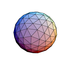
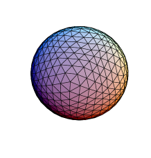
Figure 3: Approximations of the sphere by geodesic domes

For the classification of regular convex polytopes we refer to Coxeter [1]. Theorem 4.4 is proved in article [10] for the $n$-dimensional regular simplex and in article [12] for the exceptional regular polytopes, that is, for the dodecahedron and icosahedron in $3$-dimensions and for the $24$-cell, $120$-cell and $600$-cell in $4$-dimensions. For the $n$-dimensional cross polytope, namely, the analogue in $n$-dimensions of the octahedron, there is no detailed written proof in the literature, but a proof quite similar to the regular $n$-simplex case is feasible. This is because each face of an $n$-dimensional cross polytope is an $(n-1)$-dimensional regular simplex. Finally the $n$-dimensional cube case has been treated in this article (Theorem 1.1), in which case the proof is quite different from those in the other cases. Here we should also mention the important studies [2, 3, 4, 5, 6, 8] etc. of earlier times, which contain partial answers to our questions, referring to the survey [11] for a more extensive literature.

Apart from the regular figures for which symmetry plays a dominant role, polyhedral harmonics is largely open, for example, for such figures as geodesic domes in Figure 3.

References

[1]H.M.S. Coxeter,
Regular polytopes, 3rd ed., Dover, New York, 1973.
[2]L. Flatto,
Functions with a mean value property, II,
Amer. J. Math. 85 (1963), 248–270.
[3]L. Flatto,
Basic sets of invariants for finite reflection groups,
Bull. Amer. Math. Soc. 74 (1968), no. 4, 730–734.
[4]L. Flatto and M.M. Wiener,
Regular polytopes and harmonic polynomials,
Canad. J. Math. 22 (1970), 7–21.
[5]A.M. Garsia and E. Rodemich,
On functions satisfying the mean value property with
respect to a product measure,
Proc. Amer. Math. Soc. 17 (1966), 592–594.
[6]G.K. Haeuslein,
On the algebraic independence of symmetric functions,
Proc Amer. Math. Soc. 25 (1970), no. 1, 179–182.
[7]J.E. Humphreys,
Reflection groups and Coxeter groups,
Cambridge Univ. Press, Cambridge, 1990.
[8]V.F. Ignatenko,
A system of basis invariants of the group ,
J. Soviet Math. 51 (1990), no. 2, 2228–2229.
[9]K. Iwasaki,
Polytopes and the mean value property,
Discrete & Comput. Geometry 17,
(1997), 163–189.
[10]K. Iwasaki,
Regular simplices, symmetric polynomials
and the mean value property,
J. Analyse Math. 72 (1997), 279–298.
[12]K. Iwasaki, A. Kenma and K. Matsumoto,
Polynomial invariants and harmonic functions related
to exceptional regular polytopes,
Experimental Math. 11 (2002), no. 2, 313–319.
[13]I.G. Macdonald,
Symmetric functions and Hall polynomials,
2nd ed., Oxford Univ. Press, Oxford, 1995.
[14] R. Steinberg,
Differential equations invariant under finite
reflection groups,
Trans. Amer. Math. Soc. 112 (1964), 392–400.