Noisy pulses enhance temporal resolution in pump–probe spectroscopy

Abstract

Time-resolved measurements of quantum dynamics are based on the availability of controlled events (e.g. pump and probe pulses) that are shorter in duration than the typical evolution time scale of the dynamical processes to be observed. Here we introduce the concept of noise-enhanced pump–probe spectroscopy, allowing the measurement of dynamics significantly shorter than the average pulse duration by exploiting randomly varying, partially coherent light fields consisting of bunched colored noise. It is shown that statistically fluctuating fields can be superior by more than a factor of 10 to frequency-stabilized fields, with important implications for time-resolved pump-probe experiments at x-ray free-electron lasers (FELs) and, in general, for measurements at the frontiers of temporal resolution (e.g. attosecond spectroscopy). As an example application, the concept is used to explain the recent experimental observation of vibrational wave-packet motion in a deuterium molecular ion on time scales shorter than the average pulse duration.

Noise, the absence of order and correlation, is ubiquitous in nature. Typically, noise represents a nuisance or even a serious problem in experimental studies of structure or dynamics. With regard to spectroscopy applications, the laser has led to fast-paced progress by exhibiting remarkable coherence properties. Coherence helps to combat noise by inducing structure (fixed phase relations) in time or the spectral domain and thus enables applications such as high-resolution spectroscopy Udem et al. (2002), laser cooling Chu et al. (1985), and ultrafast probing of quantum dynamics on time scales down to attoseconds Hentschel et al. (2001). Recent major achievements in several fields based on such high-coherence sources have distracted from the fact that there could be beneficial aspects of temporally noisy light sources.

One example for the benefits of noise is stochastic resonance that was found to be a far-reaching concept in natural systems Wiesenfeld and Moss (1995). It has also been recently shown that noisy light fields can enhance ionization of atoms in moderately strong laser fields Singh and Rost (2007). Previous work has studied the influence of noisy pulse shapes on non-resonant autocorrelation measurements Pike and Hercher (1970) and to increase spectral resolution in linear Kinrot et al. (1995) and nonlinear Coherent Raman scattering experiments Stimson et al. (1996, 1997); Xu et al. (2008), and two-photon absorption with quantum-correlated noise Dayan et al. (2004). However, it has not been recognized that noisy pulse shapes can improve the temporal resolution in pump–probe spectroscopy for directly measuring quantum dynamics, such as molecular or electronic wave-packet motion. It is a commonly held belief that in low-order nonlinear processes, the pulse duration limits the temporal resolution for dynamical probing experiments.

Here, we introduce a new concept in time-resolved spectroscopy: using varying but correlated pairs of noisy pulse shapes to enhance temporal resolution in pump-probe experiments far beyond the average-pulse-duration limit. For an example experiment discussed in this letter, the temporal resolution is increased by a factor of 10 from 30 to 3 fs. This finding thus also creates a new paradigm in the current quest for achieving the finest temporal resolution of quantum-dynamical processes: noisy light fields as an accessible alternative if dispersive compression of broadband coherent spectra is not possible. The need to consider and rethink temporal noise has been stimulated by the development of Free-Electron Laser (FEL) Sources as FEL pulses are known to exhibit statistically varying shapes Saldin et al. (2000); Pfeifer et al. (2010). The growing field of FEL science thus provides excellent examples to demonstrate the concept. Here, we chose to describe the conceptual mechanism for the example of a sequential second-order nonlinear process, the probing of induced molecular wave-packet dynamics in a deuterium molecule. The general physical picture to understand the time-resolved pump–probe experiments with statistically varying fields is also applicable to other dynamical spectroscopy techniques. We also emphasize that the presented mechanism is universal and not even limited to optical molecular spectroscopy. It is a qualitatively new conceptual finding that can be transferred and extended to various applications in physics, technology (communications), chemistry, and the life sciences, and across various time scales and processes, wherever noisy sources of signals are involved.

The experiment discussed here was recently performed at the Free-electron LASer at Hamburg (FLASH) Jiang et al. (2010a). This XUV-pump–XUV-probe experiment investigated the two-photon double ionization (TPDI) of D₂ using FEL pulses at an energy of 38 eV, with a bandwidth of $\sim$0.53 eV FWHM, and an average pulse duration of 30 fs. In this study oscillations on a time scale of $\sim$20 fs were measured, which were initially unexpected given the longer average pulse duration of 30 fs. The variation of the temporal pulse profiles from shot to shot is illustrated in Fig. 1(a).

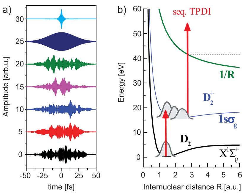
Figure 1: (Color online). The essential elements of the pump–probe light–matter interaction experiment: (a) The temporal pulse shapes of (top to bottom) a 1.12 fs short pulse, a 30 fs pulse and a set of the FEL pulses. (b) A schematic of potential-energy curves of D₂ and its cations, indicating the pathway of the sequential two-photon double-ionization (TPDI) process.

In the experiment Jiang et al. (2010a), the dynamics of the nuclear wave packet was monitored by measuring the kinetic energy release (KER) of the produced D⁺ ions as a function of a variable time delay $\tau$ between the pump and the probe pulses. Both pulses were derived out of the same FEL beam using a two-component split mirror (linearly cut in the center). The XUV-laser electric field experienced by the D₂ molecules in the interaction region is then the sum of the identical electric fields $E(t)$ of pump and time-delayed probe, translating into an intensity $I_{\tau}(t)$

$$I_{\tau}(t)=\left|E(t)+E(t+\tau)\right|^{2}.$$ (1)

In this and any other (electronic or molecular dynamics) sequential TPDI process the molecule can absorb photon 1 and photon 2 at different times $t^{\prime}$ and $t^{\prime\prime}$. As the absorption of each photon proceeds into a continuum [see Fig. 1(b)] and is far from bound-state resonances (on a scale of the pulse bandwidth), a frequency-independent rate-equation model for the ionization can be used. Hereby, the probability for each individual ionization step is proportional to the intensity $I_{\tau}(t)$. In this model, the number of doubly-ionized molecules (for the example considered here) can be calculated as

$$N_{\mathrm{total}}(\tau)\propto\int^{\infty}_{-\infty}dt^{\prime\prime}\>\int^{t^{\prime\prime}}_{-\infty}dt^{\prime}I_{\tau}(t^{\prime})I_{\tau}(t^{\prime\prime}).$$ (2)

Introducing the time difference $t_{\textrm{c}}=t^{\prime\prime}-t^{\prime}$ of the photon absorption and swapping integration order leads to

$$N_{\mathrm{total}}(\tau) \propto \int^{\infty}_{0}dt_{\textrm{c}}\int^{\infty}_{-\infty}dt^{\prime\prime}\>I_{\tau}(t^{\prime\prime}-t_{\textrm{c}})I_{\tau}(t^{\prime\prime})$$ (3)

$$= \int^{\infty}_{0}dt_{\textrm{c}}\>A^{(2)}_{\textrm{c}}(t_{\textrm{c}},\tau),$$

where $A^{(2)}_{\textrm{c}}(t_{\textrm{c}},\tau)=\int^{\infty}_{-\infty}dt\>I_{\tau}(t)\cdot I_{\tau}(t-t_{\textrm{c}})$, with $t_{\textrm{c}}$ now interpreted as correlation time, is in the following referred to as the two-dimensional autocorrelation (2dAC) function. It will be shown below that this function is a very general object in the description of sequential second-order pump–probe experiments, irrespective of measuring molecular or electronic dynamics.

In the following, we use a molecular response function $M(E_{\textrm{KER}},t_{\textrm{c}})$ to describe the measured kinetic-energy release (KER) distribution of D⁺ ions as a function of the temporal separation $t_{\textrm{c}}$ between two delta-like intensity pulses. The justification for this response function derives from the following considerations: photon 1 promotes the molecule to the D${}_{2}^{+}$ $1s\sigma_{g}$ molecular potential curve by removing one electron, while photon 2 removes the second electron to create the Coulomb-exploding D${}_{2}^{2+}$ state. In the time between the absorption of photon 1 and 2, a molecular wave packet evolves on the $1s\sigma_{g}$ state. When the second photon is absorbed, the momentary internuclear-distance distribution of the molecular wave packet will be mapped to KER by Coulomb explosion Chelkowski et al. (1999). The number of measured doubly ionized atoms with a specific kinetic-energy release and for a chosen time delay $\tau$ between pump and probe pulse is then given by

$$N(E_{\textrm{KER}},\tau)\propto\int^{\infty}_{0}dt_{\textrm{c}}\>M(E_{\textrm{KER}},t_{\textrm{c}})\;A^{(2)}_{\textrm{c}}(t_{\textrm{c}},\tau).$$ (4)

While the 2dAC function $A^{(2)}_{\textrm{c}}(t_{\textrm{c}},\tau)$ contains the information on the probe light structure (including its noisy properties), the response function $M(E_{\textrm{KER}},t_{\textrm{c}})$ thus contains the physical (quantum-dynamics) information of the system to be studied. For most frequently studied sequential processes (e.g. exciting a state and following its decoherence and decay), it could be calculated for any pump–probe scenario, also for exciting superpositions of electronic states, i.e. time-dependent electron wave packets. There, the response function could also depend on the observed photoelectron energies instead of or in addition to KER.

In the simulation, we used the partial-coherence method (PCM) Pfeifer et al. (2010) to generate a set of FEL pulses starting from the average spectrum $\overline{A}(\omega)$ measured in the $D_{2}$ experiment Jiang et al. (2010a) and a random spectral phase $\phi(\omega)$. A Gaussian envelope as filter in the time domain accounts for the average experimental FEL pulse duration of 30 fs. For comparison, we consider both a bandwidth-limited Gaussian 30 fs (FWHM) pulse and a very short pulse of 1.12 fs corresponding to the Fourier transform of the average experimental spectrum, i.e. the coherence time of the FEL pulses. Their temporal pulse profiles are shown in Fig. 1(a).

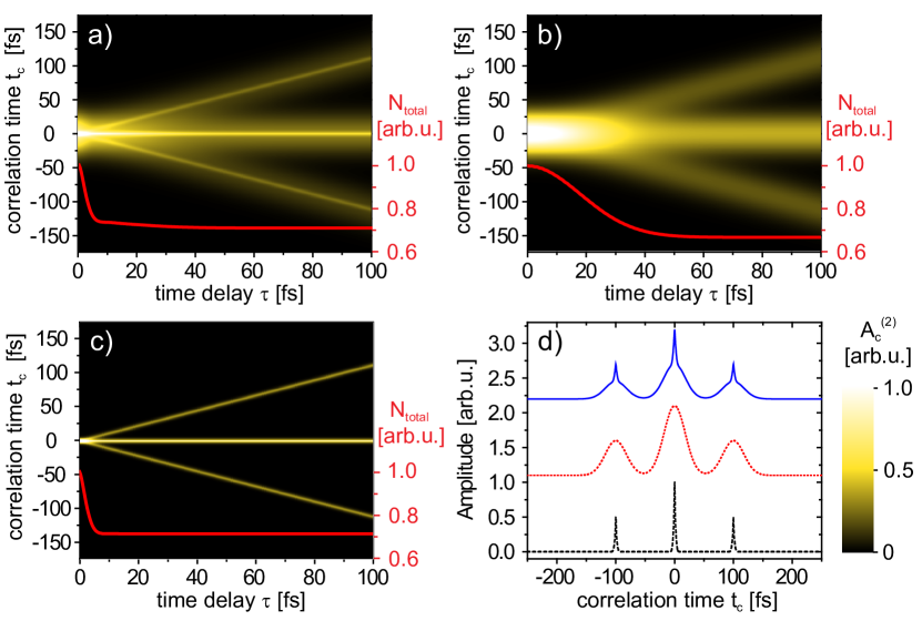
Figure 2: (Color online). Two-dimensional autocorrelation functions (2dAC) $A^{(2)}_{\textrm{c}}(t_{\textrm{c}},\tau)$, representing the intensity autocorrelation of a pair of identical (pump and probe) pulses as a function of their time delay $\tau$: (a) for a statistical average over 2000 30-fs FEL pulses, (b) for 30 fs bandwidth limited (Gaussian) pulses and (c) for 1.12 fs short pulses corresponding to the Fourier transform of the average FEL spectrum assuming a flat spectral phase. Narrow lines for $t_{\textrm{c}}=0$ and $t_{\textrm{c}}=\pm\tau$ are observed in the averaged FEL pulse case resulting from the correlated nature of the noise in pump and probe pulses on a time scale of the coherence time. These narrow temporal features are the origin of the enhanced temporal resolution. The number of doubly ionized molecules N${}_{\textrm{total}}$ is also displayed (red curves). A lineout at a time delay of 100 fs is shown in (d) for the FEL (solid blue), the bandwidth limited 30 fs (dotted red) and the 1.12 fs short pulse (dashed black).

The 2dAC functions $A^{(2)}_{\textrm{c}}(t_{\textrm{c}},\tau)$ for the three different pulses are displayed in Fig. 2(a)-(c) as well as the 2dAC functions integrated over $t_{\textrm{c}}$ which corresponds to the total number of doubly ionized molecules N${}_{\textrm{total}}$ [cf. Eq. (3)]. Since typically in the experiment the pump and probe beams do not overlap collinearly, optical-cycle interferences are washed out. We account for this by convoluting the 2dAC along the $\tau$ axis with a Gaussian of width on the order of the optical cycle duration. For the case of the bandwidth-limited 30 fs pulse, three broad lines appear, whereas these lines become very narrow for the 1.12 fs short pulse. For averaged FEL pulses, thin lines surrounded by broader pedestals occur, which are a consequence of the correlated nature of the noise on a time scale of the coherence time. Looking at N${}_{\textrm{total}}$ one can clearly see the signal enhancements for small time delays as seen before in experiments Jiang et al. (2010b). The 2dAC function for the FEL pulses closely resembles the sum of the 2dACs for the bandwidth limited 30 fs and the short 1.12 fs pulse [Fig. 2(d), see also Fig. 4(a)]. It is important to point out that the time resolution is determined by the time delay $\tau$ at which the main and the side peaks become separable in $t_{\textrm{c}}$, and also by the width of features. As a remark, the displayed 2dAC at a given $\tau$ can also be interpreted in the following way: The main peak appearing around $t_{\textrm{c}}=0~{}\textrm{fs}$ represents the case that both photons are absorbed in the same pulse whereas for the smaller peaks around $t_{\textrm{c}}=\tau$ the photons originate from different pulses. For details on the number of pulses required to obtain a smooth 2dAC function as shown here, please refer to S1 .

The model molecular response function $M(E_{\textrm{KER}},t_{\textrm{c}})$ to illustrate the application of the 2dAC concept was chosen in the following way: to describe the evolution of the molecular wave packet after absorption of the first photon, we calculated the time-dependent evolution of the molecular wave packet $\Psi(R,t_{c})$ as a function of time $t_{c}$ on the 1s$\sigma_{g}$ curve with the initial condition of $\Psi(R,t_{c}=0)$ being equal to the neutral stationary molecular ground-state wave function in D₂. The time-dependent Schrödinger equation was solved using a split-step operator approach Fleck et al. (1976); Feit et al. (1982); Pfeifer et al. (2004). The internuclear wave-packet evolution $\left|\Psi(R,t_{c})\right|^{2}$ is shown in Fig. 3(a), revealing an oscillatory dynamics on a time scale of approximately 20 fs. It is then converted to the molecular response function $M(E_{\textrm{KER}},t_{\textrm{c}})$ by using the Coulomb-explosion mapping KER $=1/R$ Chelkowski et al. (1999).

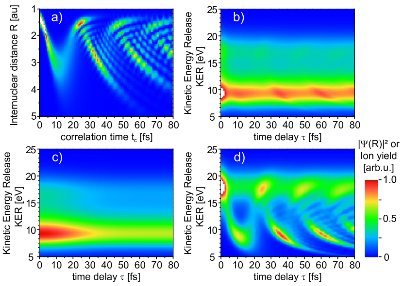
Figure 3: (Color online). The internuclear wave-packet evolution $\left|\Psi(R,t_{c})\right|^{2}$ is displayed in (a), yielding the molecular response function $M(E_{\textrm{KER}},t_{\textrm{c}})$ by employing the Coulomb-explosion mapping. Using the 2dAC functions $A^{(2)}_{\textrm{c}}(t_{\textrm{c}},\tau)$ shown in Fig. 2, the KER distributions as a function of pump–probe time delay $\tau$ (as measurable in the experiment) $N(E_{\textrm{KER}},\tau)$ can be directly obtained by integration $N(E_{\textrm{KER}},\tau)\propto\int_{0}^{+\infty}dt_{\textrm{c}}M(E_{\textrm{KER}},t_{\textrm{c}})A^{(2)}_{\textrm{c}}(t_{\textrm{c}},\tau)$. Results for $N(E_{\textrm{KER}},\tau)$ are shown for an average over $2000$ FEL pulses (b), a 30 fs bandwidth-limited pulse (c) and a 1.12 fs pulse (d). While no temporal structure is visible for the 30 fs bandwidth-limited pulse (c), the 30 fs FEL pulses, exhibiting noisy substructure, resolve the dynamics (b).

The pump–probe KER spectra $N(E_{\textrm{KER}},\tau)$ can now be calculated by using Eq. (4). For the case of the bandwidth-limited 30 fs pulse in Fig. 3(c), no dynamics can be resolved, as the $\approx$ 20 fs dynamics is washed out by the long pulse. Employing the very short 1.12 fs pulse, Fig. 3(d), the dynamics is clearly resolved. Interestingly, although the average pulse duration of the FEL is also 30 fs, the dynamics can be retrieved [see Fig. 3(b)] even for averaging over many differently structured FEL pulses. We obtain as oscillation period 23 $\pm$ 1 fs S2 which is in excellent agreement with the experimental result of 22 $\pm$ 4 fs Jiang et al. (2010a). The contribution of signal at higher KER is underestimated in our simulation for two reasons: (1) The cross-section for the ionization step from D${}_{2}^{+}$ to D${}_{2}^{2+}$ is assumed to be independent of the internuclear distance. (2) The direct (nonresonant) TPDI process is neglected which would lead to a contribution at higher KER.

It should be pointed out that the sum of the 2dACs for 1.12 fs short and 30 fs bandwidth-limited pulses is showing slightly finer ”spikes” as the FEL average 2dAC, as can be seen in Fig. 4(a) for the case $\tau=100~{}\textrm{fs}$. The obtained temporal resolution of the dynamics will thus always be slightly reduced for the case of statistically fluctuating FEL pulses, compared to the case of extremely short coherence-time duration laser pulses, but still by a factor of 10 better than the 30 fs average pulse duration [see Fig. 4(a)]. It is particularly interesting that the here-discussed phenomenon of noise-enhanced resolution is independent of the average pulse duration. Short time-scale spikes will always be present in the 2dACs as long as the coherence time of the source is sufficiently short (the average spectrum is sufficiently broad), just the ratio of spike-to-pedestal area would decrease and thus lower the usable dynamical signal vs. the background from the long pulse.

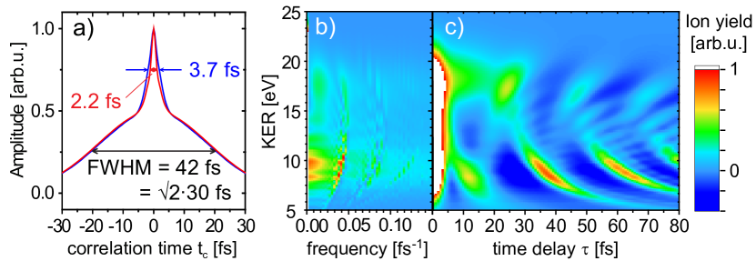
Figure 4: (Color online). (a): The central section of $A^{(2)}_{\textrm{c}}$ [from Fig. 1(d)] for FEL pulses (blue) is compared to the sum of 30 fs bandwidth limited and 1.12 fs short pulses (red). (b): Fourier transform (absolute value) of the averaged FEL KER-vs.-$\tau$ trace [Fig. 3(b)]. (c): Pump–probe scans of the FEL pulses after removing the DC component (by Fourier transform): the result approximately recovers the dynamics obtained for the coherence-time limited 1.12 fs pulses [cf. Fig. 3(d)].

The fast modulations arising by the wave-packet motion can be uncovered by means of a Fourier transform along the time delay $\tau$ axis [see Fig. 4(b)], removing the DC contribution and then transforming back into the time-delay domain [see Fig. 4(c)]. The dynamics and time-dependent shape of the molecular wave packet can thus be recovered with very high accuracy, closely resembling the expected signal for the extremely short (coherence-time limited) pulse shown in Fig. 3(d). Further detail information on how counting statistics in the experiment influences the resolution of this method can be found in S1 .

In conclusion, we presented the concept of noise-enhanced temporal resolution in pump–probe experiments. We thus also provide the physical mechanism behind the recent surprising observation of sub-pulse-duration dynamics in D₂ measured with statistically varying FEL pulses. We find that dynamical features much shorter than the average pulse duration (on the order of the coherence time of the individual pulses) can be resolved by employing the correlated nature of the noise in the pump and the probe pulses. Importantly, it should be noted that the choice of the molecular response function – also neglecting excitations to all other repulsive potential energy curves that do not result in oscillatory wave-packet dynamics – in this work was only to demonstrate the mechanism and the applicability of the 2dAC functions for well defined and statistical pulse shapes. While a different and better-suited response function can be used for the described example system of D${}_{2}^{+}$, the applicability of the presented mechanism is more general: Important consequences arise in the current race for shorter and shorter pulses and better dynamical resolutions in attosecond (and beyond) science. The mechanism could help for the case of extremely broadband high-harmonic spectra that are currently generated in experiments Seres et al. (2005); Mashiko et al. (2009); Popmintchev et al. (2009); Chen et al. (2010) and that can likely not be compressed to their bandwidth-limited few-as duration due to the absence of suitable dispersion-compensating optics. The herein presented results and novel paradigm suggest a new route: if compression is not possible, it is sufficient to statistically vary the spectral phase of the pulses. In S3 we show in detail the example for the attosecond pulse case, including the viability of the method for not fully incoherent spectral phases. This finding also has important consequences for nonlinear spectroscopy in the life sciences, as it enables time-resolved probing through moving quasi-randomly dispersive and scattering soft tissue, and could have other important applications in communications science and biological signal transmission to increase robustness of data transmission in the presence of noise.

We gratefully acknowledge funding from the Max-Planck Gesellschaft within the scope of the Max-Planck Research Group (MPRG) program.

References

- Udem et al. (2002) T. Udem, R. Holzwarth, and T. W. Hänsch, Nature 416, 233 (2002).
- Chu et al. (1985) S. Chu, L. Hollberg, J. E. Bjorkholm, A. Cable, and A. Ashkin, Phys. Rev. Lett. 55, 48 (1985).
- Hentschel et al. (2001) M. Hentschel, R. Kienberger, C. Spielmann, G. A. Reider, N. Milosevic, T. Brabec, P. Corkum, U. Heinzmann, M. Drescher, and F. Krausz, Nature 414, 509 (2001).
- Wiesenfeld and Moss (1995) K. Wiesenfeld and F. Moss, Nature 373, 33 (1995).
- Singh and Rost (2007) K. P. Singh and J. M. Rost, Phys. Rev. Lett 98, 160201 (2007).
- Pike and Hercher (1970) H. A. Pike and M. Hercher, J. Appl 41, 4562 (1970).
- Kinrot et al. (1995) O. Kinrot, I. S. Averbukh, and Y. Prior, Phys. Rev. Lett. 75, 3822 (1995).
- Stimson et al. (1996) M. J. Stimson, D. J. Ulness, and A. C. Albrecht, Chem. Phys. Lett. 263, 185 (1996).
- Stimson et al. (1997) M. J. Stimson, D. J. Ulness, and A. C. Albrecht, Journal of Raman Spectroscopy 28, 579 (1997).
- Xu et al. (2008) X. G. Xu, S. O. Konorov, J. W. Hepburn, and V. Milner, Nature Physics 4, 125 (2008).
- Dayan et al. (2004) B. Dayan, A. Pe’er, A. A. Friesem, and Y. Silberberg, Phys. Rev. Lett. 93, 023005 (2004).
- Saldin et al. (2000) E. L. Saldin, E. A. Schneidmiller, and M. V. Yurkov, The Physics of Free Electron Lasers (Springer, Berlin Heidelberg, 2000).
- Pfeifer et al. (2010) T. Pfeifer, Y. H. Jiang, S. Dusterer, R. Moshammer, and J. Ullrich, Opt. Lett. 35, 3441 (2010).
- Jiang et al. (2010a) Y. H. Jiang, A. Rudenko, J. F. Perez-Torres, O. Herrwerth, L. Foucar, M. Kurka, K. U. Kuhnel, M. Toppin, E. Plesiat, F. Morales, et al., Phys. Rev. A 81, 051402 (2010a).
- Chelkowski et al. (1999) S. Chelkowski, P. B. Corkum, and A. D. Bandrauk, Phys. Rev. Lett. 82, 3416 (1999).
- Jiang et al. (2010b) Y. H. Jiang, T. Pfeifer, A. Rudenko, O. Herrwerth, L. Foucar, M. Kurka, K. U. Kuhnel, M. Lezius, M. F. Kling, X. Liu, et al., Phys. Rev. A 82, 041403 (2010b).
- (17) See Supplemental Material at [URL will be inserted by publisher] for the discussion of the influence of statistics.
- Fleck et al. (1976) J. A. Fleck, J. R. Morris, and M. D. Feit, Appl. Phys. 10, 129 (1976).
- Feit et al. (1982) M. D. Feit, J. A. Fleck, and A. Steiger, J. Comput. Phys. 47, 412 (1982).
- Pfeifer et al. (2004) T. Pfeifer, D. Walter, G. Gerber, M. Y. Emelin, M. Y. Ryabikin, M. D. Chernobrovtseva, and A. M. Sergeev, Phys. Rev. A 70, 013805 (2004).
- (21) See Supplemental Material at [URL will be inserted by publisher] for a more detailed comparison to the experiment.
- Seres et al. (2005) J. Seres, E. Seres, A. J. Verhoef, G. Tempea, C. Strelill, P. Wobrauschek, V. Yakovlev, A. Scrinzi, C. Spielmann, and E. Krausz, Nature 433, 596 (2005).
- Mashiko et al. (2009) H. Mashiko, S. Gilbertson, M. Chini, X. Feng, C. Yun, H. Wang, S. D. Khan, S. Chen, and Z. Chang, Opt. Lett. 34, 3337 (2009).
- Popmintchev et al. (2009) T. Popmintchev, M. C. Chen, A. Bahabad, M. Gerrity, P. Sidorenko, O. Cohen, I. P. Christov, M. M. Murnane, and H. C. Kapteyn, Proc. Nat. Acad. Sci. USA 106, 10516 (2009).
- Chen et al. (2010) M. Chen, P. Arpin, T. Popmintchev, M. Gerrity, B. Zhang, M. Seaberg, D. Popmintchev, M. Murnane, and H. Kapteyn, Phys. Rev. Lett. 105 (2010).
- (26) See Supplemental Material at [URL will be inserted by publisher] for the example of attosecond pulses.