Resonant state expansion applied to planar open optical systems

Abstract

The resonant state expansion (RSE), a novel perturbation theory of Brillouin-Wigner type developed in electrodynamics [Muljarov, Langbein, and Zimmermann, Europhys. Lett., 92, 50010 (2010)], is applied to planar, effectively one-dimensional optical systems, such as layered dielectric slabs and Bragg reflector microcavities. It is demonstrated that the RSE converges with a power law in the basis size. Algorithms for error estimation and their reduction by extrapolation are presented and evaluated. Complex eigenfrequencies, electro-magnetic fields, and the Green’s function of a selection of optical systems are calculated, as well as the observable transmission spectra. In particular we find that for a Bragg-mirror microcavity, which has sharp resonances in the spectrum, the transmission calculated using the resonant state expansion reproduces the result of the transfer/scattering matrix method.

I Introduction

Recently, a novel perturbation method for the treatment of open electromagnetic systems, the resonant states expansion (RSE), has been formulated.Muljarov10 Unlike previous perturbative approachesLai90 ; Lai91 ; Leung94 ; Leung96 ; Yang10 which due to their complexity and poor convergency are limited to small perturbations, this method is shown to be suitable for perturbations of arbitrary strength and shape. It is based on the concept of resonant states (RS) of an open system, also known in quantum mechanics as GamowGamow28 or Siegert states.Siegert39 ; Moiseyev98 These states exponentially decay in time and grow in space at large distances.Baz69 Owing to their completeness inside a finite area of space, RS can be used for expanding solutions of the Maxwell equations, reducing the wave problem for the modes of the system to diagonalization of a finite complex matrix. Hence the strength and the shape of the perturbed dielectric profile that can be treated is limited only by the size of the chosen finite basis of unperturbed RS.

The idea of resonances is a cornerstone of physics, allowing to rationalize the dynamic behavior of physical systems. In open systems, excitations decay with time, endowing resonances with a spectral width. Depending on their width and separation resonances appear in measured spectra as isolated lines or merge into a continuum. The concept of RS provides a unified picture of an open system which includes all types of resonances and is an alternative to the commonplace division of the spectrum into non-decaying bound and continuum states with real energies. RS are discrete eigenstates which have complex frequencies (and equivalently energies and wave numbers) and satisfy outgoing wave boundary conditions. This corresponds to a physical situation that an open system, excited at an earlier time, looses its energy to the outside space. The imaginary part of the frequency reflects the temporal decay of the energy in the system. Owing to this leakage, the RS wave functions have tails (outgoing waves) which grow exponentially outside of the system and cannot be normalized by the usual integration of their square modulus. Instead, the normalization and orthogonality of RS is given by an integral over the finite volume of the system and the energy flux to the outside in the form of a surface term.Siegert39 ; Weinstein69

The presence of a continuum in the spectrum of a system is a significant problem for any perturbation theory. In open electromagnetic systems such a continuum is often the dominating if not the only part of the spectrum. However, going away from the real axis to the complex frequency plane, the continuum can in many cases be effectively replaced by a countable number of discrete RS which form a complete basis. Therefore, RS of a perturbed system can be expanded into the unperturbed RS. The expansion coefficients can be found by diagonalizing a complex symmetric matrix which consists of a diagonal matrix representing the bare spectrum, and the perturbation.Muljarov10 The perturbed resonant states can then be used to calculate the Green’s function of the system via its spectral representation,Newton60 ; More71 using the Mittag-Leffler theorem. The Green’s function provides the complete system response and allows to calculate observables such as emission, scattering, or transmission. This recently formulated general method of reducing the Maxwell equations for an open optical system to a linear matrix eigenvalue problem is called resonant state expansion (RSE).

The RSE has been suggestedMuljarov10 as an appropriate tool for calculation of sharp resonances in optical spectra, such as perturbed whispering gallery modes of a dielectric microsphere. Popular computational techniques in electrodynamics, such as the finite difference in time domain (FDTD)Taflove00 ; Hagness97 or the finite element methodWiersig03 ; Zienkiewicz00 ; Rahman91 adapted to such problems, require a large computational domain in time and/or space, and can produce spurious solutions.Jiang96 In particular, sharp resonances are characterized by optical modes which decay slowly in time and hence FDTD needs a large time domain. Furthermore, being applied to open systems, the finite element method either introduces a significant error when the boundary is too close, or needs to consider an excessively large domain in real space in order to describe the far-field asymptotics correctly. The RSE does not suffer from these problems because it produces the eigenstates of the system, and in particular their wave numbers, directly by diagonalization of a matrix determined by the near-field properties only.

In this paper, we apply the RSE method outlined in Section II to various planar optical systems. For such effectively one-dimensional (1D) systems efficient alternative methods exist to calculate the transmission and reflection, enabling verification of the RSE results. We investigate the accuracy with which eigenfrequencies, eigenfunctions, the Green’s function, and transmission can be reproduced. We give a method to evaluate the convergence and to extrapolate the results in Section III. We apply the RSE to a perturbed dielectric slab in Section IV with two different kind of perturbations: a wide-layer perturbation, and a $\delta$-perturbation. We find that the RSE converges to the exact solution with a power law in the basis size. As an example of a structure with a sharp resonance, we treat a Bragg mirror microcavity in Section IV.5.

II The Perturbation Method

The system of Maxwell’s equations for a planar dielectric structure with permeability $\mu=1$ surrounded by vacuum is reduced to the following wave equation:

$$\partial^{2}_{z}{\mathbb{E}}_{\nu}(z,t)=\bigl{[}\varepsilon(z)+\Delta\varepsilon(z)\bigr{]}{\partial^{2}_{t}{\mathbb{E}}_{\nu}(z,t)}\,,$$ (1)

where $\varepsilon(z)$ denotes the unperturbed dielectric profile, and $\Delta\varepsilon(z)$ the perturbation of the dielectric function. Here the transverse eigenmodes with index $\nu$ are taken with zero in-plane wave number. The electric field ${\mathbb{E}}_{\nu}(z,t)$ can be written in an harmonic form

$${\mathbb{E}}_{\nu}(z,t)=\mathcal{E}_{\nu}(z)\exp(-ic\varkappa_{\nu}t)$$ (2)

with complex frequency $c\varkappa_{\nu}$ ($c$ is the speed of light in vacuum) and amplitude $\mathcal{E}_{\nu}(z)$ satisfying the following time-independent wave equation:

$$\Bigl{\{}\partial^{2}_{z}+\bigl{[}\varepsilon(z)+\Delta\varepsilon(z)\bigr{]}\varkappa_{\nu}^{2}\Bigr{\}}\mathcal{E}_{\nu}(z)=0\,.$$ (3)

The electric field $\mathcal{E}_{\nu}(z)$ and its first derivative are continuous everywhere. RS are eigenmodes which satisfy outgoing boundary conditions, given by the form

$$\mathcal{E}_{\nu}(z)=A^{\pm}_{\nu}\exp(i\varkappa_{\nu}|z|)$$ (4)

in the surrounding vacuum with the amplitudes $A^{-}_{\nu}$ (on the left-hand side) and $A^{+}_{\nu}$ (on the right-hand side of the structure) which are generally different. In the case of a mirror-symmetric system, $A^{-}_{\nu}=A^{+}_{\nu}$ for symmetric and $A^{-}_{\nu}=-A^{+}_{\nu}$ for antisymmetric modes.

In the following, for the unperturbed RS, i.e. for $\Delta\varepsilon(z)=0$, $\mathcal{E}_{\nu}(z)$ is denoted as $E_{n}(z)$, and $\varkappa_{\nu}$ as $k_{n}$. The unperturbed RS are orthogonal and normalized according to

$$\int_{-a}^{a}\varepsilon(z){E}_{n}(z){E}_{m}(z)\,dz$$

$$-\frac{{E}_{n}(-a){E}_{m}(-a)+{E}_{n}(a){E}_{m}(a)}{i({k}_{n}+{k}_{m})}=\delta_{nm}\,,$$ (5)

where $z=\pm a$ are the positions of the boundaries of the unperturbed system. The perturbed states are written as linear combinations of the normalized unperturbed RS,

$$\mathcal{E}_{\nu}(z)=\sum_{n}c_{n\nu}\,\frac{E_{n}(z)}{\sqrt{k_{n}}}\,,$$ (6)

resulting in the linear eigenvalue problem for $\varkappa_{\nu}$ and $c_{n\nu}$

$$\sum_{m}\Big{(}\frac{\delta_{nm}}{k_{n}}+\frac{V_{nm}}{2\sqrt{k_{n}k_{m}}}\Big{)}c_{m\nu}=\frac{1}{\varkappa_{\nu}}c_{n\nu}$$ (7)

with the perturbation matrixMuljarov10

$$V_{nm}=\int_{-a}^{a}{\Delta\varepsilon(z)E_{n}(z)E_{m}(z)\,dz}\,.$$ (8)

In a dielectric system with real refractive index, the RS wave numbers $k_{n}$ have the following general property: Im $k_{n}\leq 0$ and ${\rm Re}\,k_{-n}={\rm Re}\,k_{+n}$. Additionally, in 1D systems (planar systems at normal incidence) there is always a RS with ${\rm Re}\,k_{0}=0$ and Im $k_{0}\neq 0$. We number the RS with increasing real part of their wave number, numbering the state with zero real part as state number zero. The number of RS in the unperturbed or perturbed systems is countable infinite. Therefore we always deal will a truncation of the basis of the RS, which is the only approximation of the theory. We refer to $n_{\rm{max}}$ as the truncation number for the basis so that $-n_{\rm{max}}\leq n\leq n_{\rm{max}}$. Hence the basis size $N$ is given by

$$N=2{n_{\rm{max}}}+1\,.$$ (9)

Ideally, by choosing the basis size $N$ sufficiently large, the results of the perturbation theory can be produced with any given accuracy.

The unperturbed system can be any convenient system. In the discussed 1D case, a dielectric slab in vacuum having thickness $2a$ and real dielectric constant

$$\varepsilon(z)=\left\{\begin{array}[]{cl}\epsilon_{s}&\text{for }\left|z\right|<a\\ 1&\text{otherwise }\end{array}\right.$$ (10)

is the simplest system having an analytic solution. We use it as unperturbed system in the following. The expressions for the unperturbed RS are given in the Appendix. The dielectric constant is taken to be $\sqrt{\epsilon_{s}}=1.5$ unless otherwise stated.

III Convergence and extrapolation

We introduce a method to estimate the convergence and to extrapolate the RS wave numbers calculated via the perturbation theory $\varkappa^{(N)}_{\nu}$ to their exact values $\varkappa_{\nu}^{\rm{(exact)}}$. To do so, we approximate the absolute error in each wave number as a power law in the basis size $N$:

$$\varkappa_{\nu}^{\rm{(exact)}}-\varkappa_{\nu}^{(N)}\approx K^{\prime}_{\nu}N^{\alpha^{\prime}_{\nu}}\approx K^{\prime\prime}_{\nu}N^{\alpha^{\prime\prime}_{\nu}}.$$ (11)

We assume that the exponent in the power law ($\alpha^{\prime}_{\nu}$ or $\alpha^{\prime\prime}_{\nu}$) is a real number, so that the RS wave numbers converge in a straight line in the complex plane. To determine the coefficients and exponents of the two representations in Eq. (11) we use four different values of $N$: $N_{1}<N_{2}<N_{3}<N_{4}$, where

$$N_{1}\approx\eta^{4}{N_{4}}\,,\quad N_{2}\approx\eta^{2}{N_{4}}\,,\quad N_{3}\approx\eta{N_{4}}\,,$$ (12)

producing four sets of wave numbers, with the factor $0<\eta<1$. We match states between the four sets sequentially, i.e. first $\{\varkappa^{(N_{4})}_{\nu}\}$ to $\{\varkappa^{(N_{3})}_{\nu}\}$, then $\{\varkappa^{(N_{3})}_{\nu}\}$ to $\{\varkappa^{(N_{2})}_{\nu}\}$, and finally $\{\varkappa^{(N_{2})}_{\nu}\}$ to $\{\varkappa^{(N_{1})}_{\nu}\}$. In doing this, we use the following matching algorithm (MA) between two sets of wave numbers, $\{\varkappa^{\rm{(A)}}_{\nu}\}$ and $\{\varkappa^{\rm{(B)}}_{\nu}\}$:

• Determine the distance between the complex wave numbers of all pairs with one element from $\{\varkappa^{\rm{(A)}}_{\nu}\}$ and one element from $\{\varkappa^{\rm{(B)}}_{\nu}\}$.

• Select the pair with the shortest distance, store it, and remove it from the sets.

• Repeat (b) until $\{\varkappa^{\rm{(A)}}_{\nu}\}$ or $\{\varkappa^{\rm{(B)}}_{\nu}\}$ is empty.

This procedure results in $N_{1}$ vectors $(\varkappa^{(N_{1})}_{\nu},\varkappa^{(N_{2})}_{\nu},\varkappa^{(N_{3})}_{\nu},\varkappa^{(N_{4})}_{\nu})$ of RS wave numbers. The specific factors chosen between $N_{1}$, $N_{2}$, $N_{3}$, and $N_{4}$ allow for the following analytical expressions for two sets of coefficients and exponents in Eq. (11), for each state $\nu$:

$$\alpha^{\prime}_{\nu} = \frac{1}{2\ln\eta}\ln\left(\left|\frac{{\varkappa^{(N_{4})}_{\nu}}-{\varkappa^{(N_{1})}_{\nu}}}{{\varkappa^{(N_{4})}_{\nu}}-{\varkappa^{(N_{2})}_{\nu}}}\right|-1\right),$$ (13)

$$\alpha^{\prime\prime}_{\nu} = \frac{1}{\ln\eta}\ln\left(\left|\frac{{\varkappa^{(N_{4})}_{\nu}}-{\varkappa^{(N_{2})}_{\nu}}}{{\varkappa^{(N_{4})}_{\nu}}-{\varkappa^{(N_{3})}_{\nu}}}\right|-1\right),$$ (14)

$$K^{\prime}_{\nu} = \frac{{\varkappa^{(N_{4})}_{\nu}}-{\varkappa^{(N_{2})}_{\nu}}}{{N}^{\alpha^{\prime}_{\nu}}_{2}-{N}^{\alpha^{\prime}_{\nu}}_{4}}\,,$$ (15)

$$K^{\prime\prime}_{\nu} = \frac{{\varkappa^{(N_{4})}_{\nu}}-{\varkappa^{(N_{3})}_{\nu}}}{{N}^{\alpha^{\prime\prime}_{\nu}}_{3}-{N}^{\alpha^{\prime\prime}_{\nu}}_{4}}\,.$$ (16)

For extrapolation of eigenvalues and estimation of errors we also introduce mean values $\alpha_{\nu}$ and $K_{\nu}$ defined as

$$\alpha_{\nu}=\frac{\alpha^{\prime}_{\nu}+\alpha^{\prime\prime}_{\nu}}{2}\,,\ \ \ K_{\nu}N^{\alpha_{\nu}}_{4}=\frac{K^{\prime}_{\nu}N^{\alpha^{\prime}_{\nu}}_{4}+K^{\prime\prime}_{\nu}N^{\alpha^{\prime\prime}_{\nu}}_{4}}{2}\,.$$ (17)

In order to test the quality of our power law fit, we estimate for each state $\nu$ the relative extrapolation error defined as

$$F_{\nu}=\Phi(K^{\prime}_{\nu}N^{\alpha^{\prime}_{\nu}}_{4},K^{\prime\prime}_{\nu}N^{\alpha^{\prime\prime}_{\nu}}_{4})\,,$$ (18)

where $2\Phi(X,Y)=\Gamma(X,Y)+\Gamma(Y,X)$ and

$$\Gamma(X,Y)=\left|\frac{X}{Y}-1\right|.$$ (19)

Indeed, $F_{\nu}$ has the meaning of a relative error in the power law approximation of the distance $\varkappa^{\rm{(exact)}}_{\nu}-{\varkappa^{(N_{4})}_{\nu}}$ deduced from the two sets of power law parameters. If this error is sufficiently small, $F_{\nu}<F_{\rm{max}}$, and the power law converges ($\alpha_{\nu}<\alpha_{\rm max}$), we can improve the result calculated for the largest basis size $N_{4}$ by extrapolating it towards the exact value, $\varkappa^{(N_{4})}_{\nu}\to\varkappa^{(\infty)}_{\nu}$, where the extrapolated wave vector $\varkappa^{(\infty)}_{\nu}$ is defined according to Eq. (11) as

$$\varkappa^{(\infty)}_{\nu}=\varkappa^{(N_{4})}_{\nu}+K_{\nu}N^{\alpha_{\nu}}_{4}.$$ (20)

Otherwise, the power law is not describing the convergence well. We then use the absolute variation scaled to the system size to evaluate if the state has sufficiently converged

$$M_{\nu}=\max_{i=1,2,3}\left|{\varkappa^{(N_{4})}_{\nu}}-{\varkappa^{(N_{i})}_{\nu}}\right|a\,.$$ (21)

We use state $\nu$ for the calculation of the Greens function if its relative or absolute error is sufficiently small, i.e. if one of the two selection criteria (SC) is met:

1. extrapolation error $F_{\nu}|K_{\nu}N_{4}^{\alpha_{\nu}}|a<M_{\rm{max}}$ provided that $F_{\nu}<F_{\rm{max}}$ and $\alpha_{\nu}<\alpha_{\rm max}$ ;

2. absolute error $M_{\nu}<M_{\rm{max}}$ .

For the results shown in the present paper we used $M_{\max}=0.1$, $F_{\rm{max}}=1$, $\alpha_{\max}=-0.5$, and $\eta=2^{-1/4}$.

IV Results

IV.1 Wide-layer perturbation

The perturbation being considered in this section is given by

$$\Delta\varepsilon(z)=\left\{\begin{array}[]{cl}\Delta\epsilon&\text{for\ \ }a/2\leq z\leq a\,,\\ 0&\text{otherwise }\end{array}\right.$$ (22)

with $\Delta\epsilon=10$. The profiles of the unperturbed and perturbed dielectric constants are shown in Fig. 1. The analytic solutions of the time-independent Maxwell’s equations using the RS boundary conditions are given in Appendix A, both for the unperturbed and the perturbed systems, along with the matrix elements $V_{nm}$ of the perturbation.

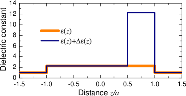
Figure 1: Dielectric constants of the unperturbed slab $\varepsilon(z)$ and a slab with a wide perturbation $\varepsilon(z)+\Delta\varepsilon(z)$. The distance $z$ is in units of the half width $a$ of the slab.

Using the procedure introduced in Section III we calculate four sets of perturbed wave numbers and extrapolate $\varkappa_{\nu}$ according to Eq. (20). We also calculate the exact wave numbers ${\varkappa^{\rm{(exact)}}_{\nu}}$ and match up exact and perturbed states using the MA. The resulting exact and extrapolated eigenvalues ${\varkappa^{{(\infty)}}_{\nu}}$ are shown in the inset of Fig. 2, together with the unperturbed wave vectors. We measure the errors in ${\varkappa^{{(\infty)}}_{\nu}}$ relative to ${\varkappa^{\rm{(exact)}}_{\nu}}$ by $\Gamma(\varkappa^{(\infty)}_{\nu},\varkappa^{\rm(exact)}_{\nu})$ and compare it with $\Gamma(\varkappa^{(N_{4})}_{\nu},\varkappa^{\rm(exact)}_{\nu})$ to evaluate the extrapolation method. The results are shown in Fig. 2. We see that the relative error of the RS wave number is generally reduced by extrapolation by more than one order of magnitude.

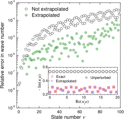
Figure 2: Relative errors $\Gamma(\varkappa^{(\infty)}_{\nu},\varkappa^{\rm(exact)}_{\nu})$ and $\Gamma(\varkappa^{(N_{4})}_{\nu},\varkappa^{\rm(exact)}_{\nu})$ of the RS wave vectors calculated via the RSE for the perturbation shown in Fig. 1, with and without extrapolation, respectively, for $N_{4}=801$. Inset: unperturbed and perturbed RS wave numbers; the latter are calculated analytically (empty squares) and via the RSE with extrapolation (crosses).

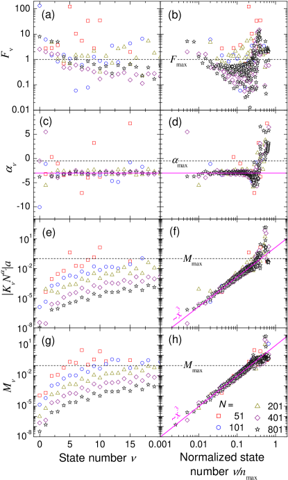
Figure 3: Power law parameters and error estimates for the wide perturbation. (a),(b): Relative extrapolation error $F_{\nu}$. (c),(d): exponent $\alpha_{\nu}$ in the power law fit. (e),(f): absolute errors $K_{\nu}N^{\alpha_{\nu}}$ and (g),(h): $M_{\nu}$ as function of the the state number $\nu$, calculated for different basis size $N$. The right panels display the data versus the state number $\nu$ normalized to its maximum value $n_{\rm max}=(N-1)/2$. Straight magenta lines are $\alpha=-3$ (c),(d) and power law fits (h),(f).

The coefficients and exponents of the power law fit give us information about the convergence properties of the perturbed RS. For the wide perturbed layer they are shown in Fig. 3. We see in Fig. 3 (a) that states close to the origin in complex wave number space (and having small state number values) are not described well by the power law ($F_{\nu}$ is larger than $F_{\rm{max}}$), even though Fig. 2 suggests that these states are well converged. This is reflected in the small absolute error $M_{\nu}$ shown in Fig. 3(g),(h), passing the SC. We also see that for higher wave-number states passing the relative SC the exponent in the power law is close to $\alpha=-3$ [horizontal lines in Fig. 3 (c),(d)], in accordance with the findings in Ref. Muljarov10, .

Furthermore, the absolute errors $K_{\nu}N^{\alpha_{\nu}}$ and $M_{\nu}$ show universal dependencies on the normalized state number $\nu/n_{\rm max}$, as shown in Fig. 3 (f) and (h). This provides us with a scaling law of the absolute errors versus the state number:

$$M_{\nu}\propto(\nu/N)^{3}\,.$$ (23)

This cubic scaling is shown in Fig. 3 (f),(h) by straight magenta lines. The power law exponent $\alpha$ also shows a universal dependency on the normalized state number, being $\alpha=-3$ for $\nu/n_{\max}\lesssim 0.2$ as can be seen in Fig. 3 (d). In this region the states pass the relative SC and are extrapolated.

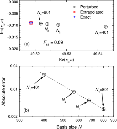
Figure 4: (a) Wave number of the perturbed state $\nu=63$ calculated with different basis sizes $N$ and extrapolated to the exact value. (b) Absolute “exact” error $|\varkappa^{\rm(exact)}_{63}-\varkappa^{(N)}_{63}|$ for different $N$ (squares) and a power law fit (dashed line).

An example of how the power law is applied to extrapolate the wave number of a particular state $\nu=63$ is given in Fig. 4 (a). Clearly, the extrapolation leads to a considerable improvement of the accuracy compared to wave number calculated with the maximum matrix size $N_{4}$. This is due to the good power law convergence as shown in Figure 4 (b), seen by the straight line connecting the “exact” errors $|\varkappa^{\rm(exact)}_{\nu}-\varkappa^{(N_{i})}_{\nu}|$ for the four basis sizes.

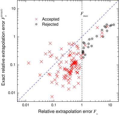
Figure 5: “Exact” relative extrapolation error $F_{\nu}^{\rm(exact)}$ versus relative extrapolation error $F_{\nu}$ for both accepted and rejected states, for $N_{4}=801$. The blue dashed line shows the anticipated behavior $F_{\nu}^{\rm(exact)}\approx F_{\nu}$.

The exact errors are only available if the exact solution is known, but in this ideal case we do not need the RSE. In a realistic case for which no such solution is known, we need to estimate the error of the power law extrapolation, which we do using the extrapolation SC and Eq. (18). In order to check how good this estimation is, we compare $F_{\nu}$ with the exact relative extrapolation error $F_{\nu}^{\rm(exact)}=\Phi(K_{\nu}N^{\alpha_{\nu}}_{4},\varkappa^{\rm(exact)}_{\nu}-\varkappa^{(N_{4})}_{\nu})$. Such a comparison is shown in Fig. 5 for all states with $\alpha_{\nu}<-0.5$. We can see that the exact error $F_{\nu}^{\rm(exact)}$ is typically overestimated by $F_{\nu}$, and for all states with $F_{\nu}<F_{\rm max}$ we have $F_{\nu}^{\rm(exact)}<1$, i.e. the extrapolation is improving the error. $F_{\nu}$ can thus be used reliably to verify the convergency and power law extrapolation.

IV.2 Electric fields

The electric fields (EF) $\mathcal{E}_{\nu}(z)$ of the perturbed RS calculated via the exact formula Eq. (36) are shown in Fig. 6 for a few lowest states in comparison with $E_{n}(z)$, the EF of the unperturbed RS, given by Eq. (32). The perturbed RS are normalized as in Eq. (5). In particular, their orthonormality condition reads

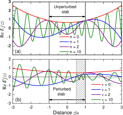
Figure 6: Real part of the normalized electric field of a few lowest energy RS of the unperturbed slab (a) and of the perturbed slab (b).

$$\int_{-a}^{a}\varepsilon_{p}(z)\mathcal{E}_{\nu}(z)\mathcal{E}_{\mu}(z)\,dz$$

$$-\frac{\mathcal{E}_{\nu}(-a)\mathcal{E}_{\mu}(-a)+\mathcal{E}_{\nu}(a)\mathcal{E}_{\mu}(a)}{i({\varkappa}_{\nu}+{\varkappa}_{\mu})}=\delta_{\nu\mu}\,,$$ (24)

where $\varepsilon_{p}(z)=\varepsilon(z)+\Delta\varepsilon(z)$ is the perturbed dielectric profile. All unperturbed states have the same imaginary part of their wave vectors (see the inset in Fig. 2) and thus their fields have all the same envelope, exponentially growing outside the slab, with the higher-$n$ states oscillating more rapidly, see Fig. 6 (a). In the perturbed system, the envelopes are different due the varying Im $\varkappa_{\nu}$. Also, as can be seen in Fig. 6(b), the frequency of the oscillations increases in the perturbed (denser) layer, and their amplitudes change at the same time.

The perturbation theory fully reproduces the EF of the RS, both inside and outside the slab. Inside the slab, the EF is given by the expansion in Eq. (6) with the coefficients $c_{n\nu}$ diagonalizing the matrix in Eq. (7). Outside the slab, the fields are given by Eq. (4) in which the perturbed wave vectors $\varkappa_{\nu}$ assign the proper exponential growth and oscillations of the EF in vacuum, while the amplitudes $A_{\nu}^{\pm}$ are found by comparing Eqs. (4) and (6) and using the continuity of the EF through the boundaries. To quantify how well the perturbation theory reproduces the EF of a RS, we calculate its root mean square (RMS) deviation within the system defined by

$$\Delta_{\nu}=\sqrt{\frac{\int^{a}_{-a}\bigl{|}\mathcal{E}^{(N)}_{\nu}(z)-\mathcal{E}^{\rm(exact)}_{\nu}(z)\bigr{|}^{2}\,dz}{\int^{a}_{-a}\bigl{|}\mathcal{E}^{\rm(exact)}_{\nu}(z)\bigr{|}^{2}\,dz}}\,.$$ (25)

The results are shown in Fig. 7, where we have matched exact and perturbed RS using the MA and plotted $\Delta_{\nu}$ for different basis sizes $N$. We see that the trend in accuracy with state number and the basis size is the same as in Fig. 3(e),(g), and the RMS deviation versus the normalized state number also shows a universal dependence similar to those in Fig. 3(f),(h). However, the EF is in general less well reproduced than the wave numbers and the power law $\Delta_{\nu}\propto(\nu/N)^{3}$ is observed only in the interval of $0.05<\Delta_{\nu}<0.2$.

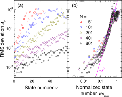
Figure 7: Root mean square deviation of the RS electric field $\mathcal{E}^{N}_{\nu}$ from its exact value $\mathcal{E}^{\rm(exact)}_{\nu}$ versus the state number $\nu$ (a) and normalized state number $\nu/n_{\rm{max}}$ (b), calculated for different basis sizes $N$. The straight magenta line in (b) is a cubic law fit.

IV.3 Green’s function and transmission

The Green’s function (GF) is an important quantity which fully characterizes the response of an optical system, determining its scattering and transmission. For the slab with a wide perturbed layer given by Eqs. (10) and (22), the GF $G(z,z^{\prime};k)$ which satisfies the equation

$$\Big{\{}\partial^{2}_{z}+\bigl{[}\varepsilon(z)+\Delta\varepsilon(z)\bigr{]}k^{2}\Bigr{\}}G(z,z^{\prime};k)=\delta(z-z^{\prime})$$ (26)

and outgoing boundary conditions can be calculated analytically. Note that when calculating observables, $k$ is real as it is given by the vacuum wave number of an external driving field. The GF is calculated using its spectral representation,Newton60 ; More71 ; Muljarov10

$$G(z,z^{\prime};k)=\sum_{\nu}\frac{\mathcal{E}_{\nu}(z)\mathcal{E}_{\nu}(z^{\prime})}{2k(k-{\varkappa}_{\nu})}\,,$$ (27)

in which the EF $\mathcal{E}_{\nu}(z)$ and the RS wave numbers $\varkappa_{\nu}$ are calculated numerically via the RSE. For the wave numbers $\varkappa_{\nu}$, we use the extrapolated values Eq. (20).

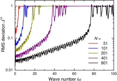
Figure 8: The root mean square deviation in the GF $\Delta^{\rm{GF}}$ as a function of the wave number of the driving field $k$, calculated via the RSE for different basis sizes $N$.

In light of the importance of the GF and its further usage for calculation of observables, we compare $G^{(N)}$, the GF calculated by RSE with basis size $N$ and Eq. (27), to its exact analytic form $G^{\rm{(exact)}}$, again using the RMS deviation as given by

$$\Delta^{\rm{GF}}=\sqrt{\frac{\int^{a}_{-a}\!\int^{a}_{-a}\bigl{|}G^{(N)}(z,z^{\prime})-G^{\rm{(exact)}}(z,z^{\prime})\bigr{|}^{2}\,dzdz^{\prime}}{\int^{a}_{-a}\!\int^{a}_{-a}\bigl{|}G^{\rm{(exact)}}(z,z^{\prime})\bigr{|}^{2}\,dzdz^{\prime}}}\,.$$ (28)

Such a comparison is shown in Fig. 8 for different basis sizes $N$. Increasing the basis size has two effects on the GF: (i) it improves the GF error at a given $k$ and (ii) widens the $k$-range of the GF with small error. The latter is due to a larger wave-number range of poles in the GF, Eq. (27), being reproduced for large $N$.

Both expansions Eqs. (6) and (27), for the EF and for the GF, are valid only inside the slab or on its borders and are not suitable for the vacuum area where the EF of the RS grow exponentially. The GF itself is, however, regular on the real $k$-axis. Moreover, in vacuum, it always has a simple analytic form of a plane wave with the amplitude that can be deduced from values inside the slab, Eq. (27), using the continuity of the GF when passing through the interfaces. In this way, the GF can be calculated at any point of the $(z,z^{\prime})$ space, inside or outside the slab.

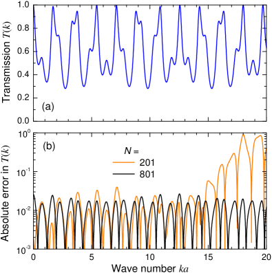
Figure 9: (a) Light transmission through the slab with a wide-layer perturbation Eq. (22). (b) Absolute error in the transmission calculated using the analytic form of $T(k)$ and numerical values from the RSE for two different simulations.

The delta-function in Eq. (26) plays the role of a source of plane waves generated at the point $z^{\prime}$ and propagating in both directions, away from the source. The GF then has the meaning of the system’s response on such a plane-wave excitation. This can be used to derive a formula for the transmission in terms of the GF. To do this, we place the source of strength $2ik$ just outside the slab at $z^{\prime}=-a$, in order to produces two plane wave of amplitude 1. One of these waves is transmitted trough the slab, and just after the slab at point $z=a$ the intensity of the EF (which does not change with further increase of $z$) is given by

$$T(k)=\left|2kG(a,-a;k)\right|^{2}$$ (29)

and is called transmission.

We calculate the transmission using Eqs. (27) and (29) for the GF taken to be either numerical $G^{(N)}$ or analytical $G^{\rm{(exact)}}$. This allows us to calculate the absolute error in the transmission, $|T^{(N)}-T^{\rm(exact)}|$, which is shown in Fig. 9(b). The transmission itself is shown in Fig. 9(a) and has a profile which is fully determined by the pole structure of the GF. The RS which contribute in this frequency range can be seen in the inset to Fig. 2. We see that the error of the transmission has a similar magnitude and scaling with $N$ as the GF itself, as can be expected from Eq. (29).

IV.4 $\delta$-perturbation

We now move from a wide perturbation to a very narrow and strong one, like a thin metal film on a dielectric. Such a perturbation is described by

$$\Delta\varepsilon(z)=w\epsilon_{d}\delta(z-a/2)$$ (30)

with the delta-scatter strength $w\epsilon_{d}=-0.1a$. Physically, this perturbation corresponds to a thin layer of the dielectric constant changed by $\epsilon_{d}$, which is placed at $z=a/2$ and has a width $w$ much narrower than the shortest wavelength of the resonant modes used in the basis. The dielectric profile for the system with the $\delta$-perturbation is shown in Fig. 10.

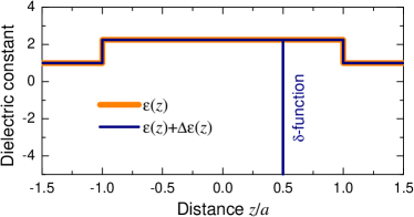
Figure 10: Dielectric constants of the unperturbed slab $\varepsilon(z)$ and a slab with a $\delta$-perturbation $\varepsilon(z)+\Delta\varepsilon(z)$. The distance $z$ is in units of the half width $a$ of the slab.

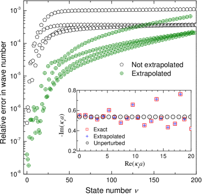
Figure 11: As Fig. 2, but for the $\delta$-perturbation shown in Fig. 10.

As in the case of a wide-layer perturbation considered in Section IV.1 we plot and compare in Figs. 11–14 the RS wave numbers, calculated exactly and via the RSE with and without extrapolation, as well as the parameters of the power law fit and relative and absolute errors which we also need for the quality check of our simulation and extrapolation. The analytic solutions for the $\delta$-perturbation and its matrix elements are given in the Appendix A.

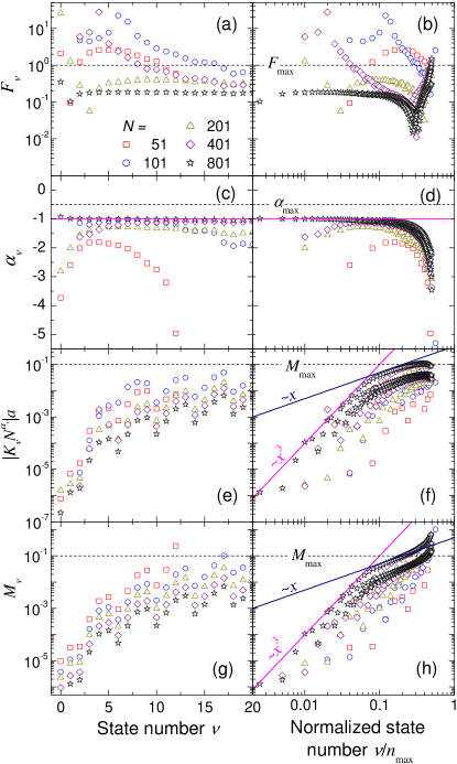
Figure 12: As Fig. 3 but for the $\delta$-perturbation shown in Fig. 10. The horizontal magenta lines in panels (c) and (d) are $\alpha=-1$ lines.

We see in Fig. 11 that the extrapolation reduces the relative error by 1-2 orders of magnitude. The integral strength of the perturbation is much (almost two orders of magnitude) weaker than in the case of the wide layer considered in Section IV.1. However, the convergence is much slower in the case of the $\delta$-perturbation. We see in Fig. 12(c),(d) that for large $N$ the power law exponent is close to $\alpha_{\nu}=-1$. This is to be expected as the $\delta$-perturbation does not have a finite width. The matrix elements $V_{nm}$, though oscillating, have no decrease with increasing wave number (or index $n$) which leads to a much stronger mixing of states compared to the wide layer perturbation. Indeed, in the wide layer case, states with higher indices are less important due to the rapid oscillation of their wave functions, so that the matrix elements scale as $V_{nm}\propto 1/n$ (for $n\gg m$). Using the second-order Rayleigh-Schrödinger perturbation theory and the explicit form Eqs. (A.3) and (43) of the matrix elements $V_{nm}$, we can show that the wave number corrections scale as $1/N$ and $1/N^{3}$ for the $\delta$- and wide-layer perturbations, respectively, in accordance with Figs. 3(d) and 12(d).

In the case of the $\delta$-perturbation, the absolute errors shown in Fig. 12(f,h) as functions of the normalized state number do not display any universal curves, still for small $\nu/N$ approaching asymptotically a cubic law in the state number $\nu$ (magenta lines). Thus we conclude that in this case $M_{\nu}\propto\nu^{3}/N$ [compare with Eq. (23)]. At larger values of $\nu/N$ this dependence transforms into a linear one, $M_{\nu}\propto\nu/N$ (blue lines). Because of the slow ($1/N$) convergence, the extrapolation gives a huge improvement as is clear from Fig. 13 and demonstrates its necessity in the particular case of the $\delta$-perturbation.

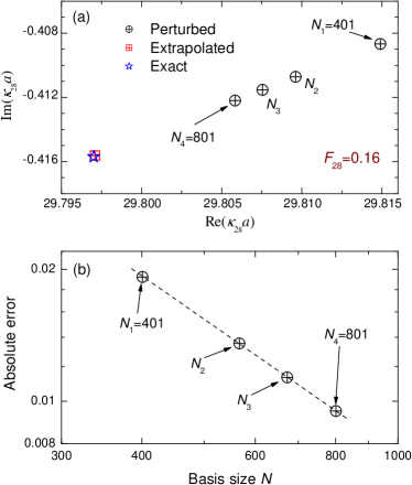
Figure 13: As Fig. 4, but for the $\delta$-perturbation shown in Fig. 10 and state number $\nu=28$.

At the same time, the relative extrapolation error is predicted within an order of magnitude, as can bee seen in Fig. 14. For the majority of RS, $F^{\rm(exact)}_{\nu}<F_{\nu}$, the exact values $F^{\rm(exact)}_{\nu}$ being significantly overestimated. However, for a large class of solutions it turns out to be highly underestimated. The systematic deviation seen Fig. 14 in estimating the relative extrapolation error though $F_{\nu}$ may be a result of the systematic variation in the power law exponent $\alpha_{\nu}$ well seen in Fig. 12(c),(d). Hence it is generally advisable when studying convergence with our method to run simulations with a variety of $N_{4}$ parameters in order to establish over what range of $N_{4}$ the power law is applicable for the given strength of perturbation.

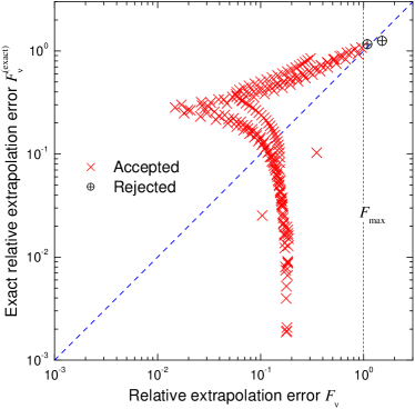
Figure 14: As Fig. 5, but for the $\delta$-perturbation shown in Fig. 10.

We were also able to simulate a $\delta$-perturbation outside the perturbed slab by taking the unperturbed slab to include the position of the delta scatterer and thus the perturbation consisting of a superposition of a $\delta$-perturbation and a wide layer compensating the difference in the dielectric constants between the vacuum and the unperturbed slab. In this case we did obtain convergence of the perturbed wave numbers to the exact solution. However, for a $\delta$-perturbation outside of the unperturbed slab or exactly on the border, the simulation does not converge to the correct solution. This is to be expected since in this case the perturbed RS contain waves reflected from the external perturbation, which are waves propagating towards the slab. Such incoming waves are not part of the basis of unperturbed RS, and thus cannot be reproduced by an expansion in this basis.

IV.5 Microcavity

To evaluate the RSE in presence of sharp resonances, we use a Bragg-mirror microcavity (MC), which consists of a Fabry-Pérot cavity of thickness $L_{C}$ and refractive index $n_{C}$ surrounded by distributed Bragg reflectors (DBRs). The DBRs consist of $P$ pairs of dielectric layers with alternating high ($n_{H}=3.0$) and low ($n_{L}=1.5$) refractive index. In order to a have sharp cavity mode at a given wavelength $\lambda_{C}$, these alternating layers have to be of quarter wavelength optical thickness, and the optical thickness of the cavity has to be a multiple of half the wavelength. We take $L_{C}=\lambda_{C}/2$. An example of the dielectric profile of such a system with $P=3$ is shown in Fig. 15.

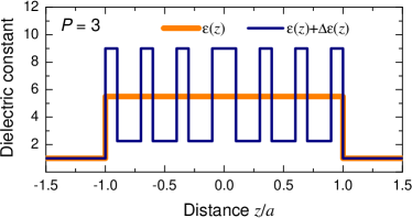
Figure 15: Dielectric profiles of a planar microcavity having $P=3$ pairs of Bragg mirrors on each side (blue line) and an unperturbed dielectric slab (orange line).

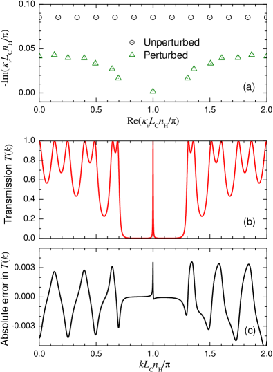
Figure 16: (a) Wave vectors $\varkappa_{\nu}$ of the resonant states of a microcavity with $P=3$ pairs of Bragg mirrors on each side calculated via RSE with $N=801$. (b) Microcavity transmission as a function of the normalized wave vector of the incoming light; $L_{C}$ and $n_{C}$ are the cavity thickness and refractive index. (c) The difference in the transmission calculated via RSE and using the scattering matrix method.Tikhodeev02

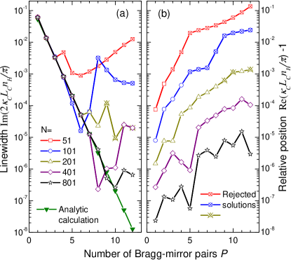
Figure 17: The FWHM (a) and the position of the cavity mode (b) calculated analytically and via the RSE for different number of pairs $P$ of Bragg mirrors on each side of the microcavity. $N$ is the basis size used in the RSE. Where possible, extrapolated wave numbers have been used. Crossed rectangles for $N=51$ indicate states which are rejected by the SC.

The RS of a MC are calculated using the RSE. The RS wave vectors and the transmission through the MC are shown in Fig. 16(a),(b). For reference, the unperturbed eigenvalues are also included in Fig. 16(a). The unperturbed system taken for the RSE is again a dielectric slab which dielectric constant $\varepsilon(z)$ can be seen in Fig. 15. Throughout this section the outer boundaries of the MC and the unperturbed slab coincide, and we choose $\epsilon_{s}=5.5$ which is between $n_{L}^{2}$ and $n_{H}^{2}$, providing good convergence. $\epsilon_{s}$ could be further optimized for best convergence of the RSE. In order to verify the transmission calculated by the RSE, we use the scattering matrix methodTikhodeev02 which is a straightforward and precise way of calculating the optical properties of a planar system. Figure 16(c) demonstrates a good agreement between the two calculations.

Clearly, there is a one-to-one correspondence between the RS wave vectors in Fig. 16(a) and the MC transmission in Fig. 16(b). Namely, the real part of the wave vectors corresponds to the positions of the peaks in the transmission while the imaginary part gives their line widths. This is well understood in view of the spectral representation of the Green’s function Eq. (27) used for the calculation of the transmission via Eq. (29).

One of the modes shown in Fig. 16(a) is rather isolated and has imaginary part much smaller than the others. This mode, $\varkappa_{C}$, satisfies the Fabry-Pérot resonance condition Re $\varkappa_{C}=\pi/(L_{C}n_{C})$ and is called the cavity mode. For the wave vector $k$ of incoming light close to this resonance condition, $k\approx\pi/(L_{C}n_{C})$, the Greens’ function Eq. (27) is dominated by a single term corresponding to this narrow mode. As a consequence, there is a sharp peak in the center of a wide stop-band seen in the transmission in Fig. 16(b). For sufficiently large $P$ an analytic approximation for its full width at half maximum (FWHM) is known,Savona95

$$\Delta k=\frac{4n_{\rm ext}}{n_{C}^{2}}\left(\frac{n_{L}}{n_{H}}\right)^{2P}\frac{1}{\displaystyle L_{C}+\frac{\lambda_{C}}{2}\,\frac{n_{L}n_{H}}{n_{C}(n_{H}-n_{L})}}\,,$$ (31)

which we use to compare with the RSE calculation. With the refractive index of the external material $n_{\rm ext}=1$ and using $\lambda_{C}=2L_{C}$ and $n_{C}=n_{H}$, Eq. (31) reduces to $\Delta k=4(n_{H}-n_{L})(n_{L}/n_{H})^{2P}/(L_{C}n_{H}^{3})$. Comparison of the above formula with the RSE result for the cavity mode is given in Fig. 17, for different number of Bragg-mirror pairs $P$ and for different basis size $N$ in the RSE. Figure 17 demonstrates that RSE is capable of giving both the correct width and location of sharp resonances in the transmission profile, if a large enough basis is used, in spite of there being no sharp resonances in the basis. As the basis size is enlarged, the width and the peak location of the cavity mode converge to the analytic values. The fact that for a fixed $N$ the cavity mode position and the width are predicted worse for larger $P$ is explained by our choice of the unperturbed slab which always has exactly the same thickness as the Bragg-mirror MC. With the number of Bragg-mirrors increasing, the field inside the MC oscillates more rapidly (also shifting the cavity mode towards higher frequencies) that requires a larger number of RS to be taken into account in order to produce results on the same level of accuracy. We have verified (not shown) that the errors become independent of $P$, if one and the same constant width of the unperturbed slab is used for different values of $P$.

V Summary

The resonant state expansion has been implemented and validated in planar open optical systems reducible to effective one-dimensional systems. A reliable method of calculation of resonant states, and in particular their wave numbers, electric fields, as well as the Green’s function and the transmission of such systems, has been developed and demonstrated.Code It includes estimation of the accuracy and convergency of calculations and in particular extrapolation of the eigen-wavevectors towards their exact values which are generally not available. Particular examples which illustrate the general method and the developed algorithm include a dielectric slab with wide-layer and $\delta$-perturbations as well as an optical microcavity having different number of Bragg mirrors. In these examples, a comparison with exact solutions has been made in order to verify the approach. In all three systems the resonant states and the transmission are reproducible to any required accuracy by the resonant state expansion. The wave vectors of resonant states are the most essential part of the calculation as they most strongly affect the optical properties of the system through the poles of the Green’s function. The extrapolation of the wave vectors using the power law in the basis size, which has been developed and demonstrated, significantly improve the accuracy of calculations, by one or two orders of magnitude. Application of the method to two and three-dimensional systems will be reported in future works.

Appendix A Analytic calculation of resonant states and perturbation matrices

A.1 Resonant states of the unperturbed slab

Solving the wave equation Eq. (3) with $\Delta\varepsilon(z)=0$ and the profile of the dielectric constant $\varepsilon(z)$ given by Eq. (10), the electric field of RS $n$, normalized according to Eq. (5), takes the form

$$E_{n}(z)=\left\{\begin{array}[]{lll}(-1)^{n}A_{n}e^{-ik_{n}z}\,,&&z<-a\,,\\ B_{n}[e^{i\sqrt{\epsilon_{s}}k_{n}z}+(-1)^{n}e^{-i\sqrt{\epsilon_{s}}k_{n}z}]\,,&&|z|\leq a\,,\\ A_{n}e^{ik_{n}z}\,,&&z>a\,,\end{array}\right.$$ (32)

where

$$A_{n}=\frac{e^{-ik_{n}a}}{\sqrt{a(\epsilon_{s}-1)}}\,,\qquad B_{n}=\frac{(-i)^{n}}{2\sqrt{a\epsilon_{s}}}\,.$$ (33)

The RS wave vectors are given by

$$k_{n}=\frac{1}{2a\sqrt{\epsilon_{s}}}(\pi n-i\ln\gamma),\qquad n=0,\,\pm 1,\,\pm 2,\,...\,,$$ (34)

with

$$\gamma=\frac{\sqrt{\epsilon_{s}}+1}{\sqrt{\epsilon_{s}}-1}\,,$$ (35)

all having the same imaginary part.

A.2 Resonant states of a slab perturbed by a wide dielectric layer

The exact solutions of the wave equation Eq. (3) for the system with the perturbation given by Eq. (22) and outgoing boundary conditions has the form

$$\mathcal{E}^{\rm{(exact)}}_{\nu}(z)=\left\{\begin{array}[]{ll}A_{\nu}e^{-i\varkappa_{\nu}z}\,,&z<-a\,,\\ B_{\nu}e^{i\sqrt{\epsilon_{s}}\varkappa_{\nu}z}+C_{\nu}e^{-i\sqrt{\epsilon_{s}}\varkappa_{\nu}z}\,,&{-a}\leq z\leq b\,,\\ D_{\nu}e^{i\sqrt{\epsilon_{p}}\varkappa_{\nu}z}+E_{\nu}e^{-i\sqrt{\epsilon_{p}}\varkappa_{\nu}z}\,,&b\leq z\leq a\,,\\ H_{\nu}e^{i\varkappa_{\nu}z}\,,&z>a\,,\\ \end{array}\right.$$ (36)

where $\epsilon_{p}=\epsilon_{s}+\Delta\epsilon$, and $b=a/2$. The coefficients in Eq. (36) are found from the continuity of the electric field and its derivative and the normalization condition Eq. (24). The complex-valued RS wave numbers $\varkappa_{\nu}$ are found by solving a secular equation following from the boundary conditions:

$$\beta\gamma f(k)g(k)-1=\frac{\beta-\gamma}{\beta\gamma-1}\Bigl{[}\beta g(k)-\gamma f(k)\Bigr{]}\,,$$ (37)

where

$$\beta=\frac{\sqrt{\epsilon_{p}}+1}{\sqrt{\epsilon_{p}}-1}\,,$$ (38)

and the functions $f(k)$ and $g(k)$ are defined as

$$f(k)=e^{-2i\sqrt{\epsilon_{s}}k(a+b)}\,,\ \ \ g(k)=e^{-2i\sqrt{\epsilon_{s}}k(a-b)}\,.$$ (39)

We solve Eq. (37) using the Newton-Raphson method to find $k=\varkappa_{\nu}^{\rm{(exact)}}$.

A.3 Matrix elements of the wide-layer perturbation

Using Eq. (8) and basis functions Eq. (32) we calculate $V_{nm}$ for the wide-layer perturbation Eq. (22) to be

$$V_{nm}=\frac{\Delta\epsilon}{\epsilon_{s}}\,\frac{1}{4ia\sqrt{\epsilon_{s}}}\Bigl{[}\!\!\!\!\!\! (-i)^{n+m}\eta(k_{n}+k_{m},z)$$

$$+(-i)^{n-m}\eta(k_{n}-k_{m},z)$$

$$+(-i)^{-n+m}\eta(-k_{n}+k_{m},z)$$

$$+(-i)^{-n-m}\eta(-k_{n}-k_{m},z)\Bigr{]}_{b}^{a}\,,$$

for $n\neq m$ and

$$V_{nn}=\frac{\Delta\epsilon}{\epsilon_{s}}\,\left\{\frac{a-b}{2a}+(-1)^{n}\frac{\bigl{[}\eta(2k_{n},z)+\eta(-2k_{n},z)\bigr{]}_{b}^{a}}{4ia\sqrt{\epsilon_{s}}}\right\}$$ (41)

for $n=m$, where $\eta(k,z)=e^{i\sqrt{\epsilon_{s}}kz}/k$.

A.4 Resonant states of a slab perturbed by a delta scatterer

In the case of a $\delta$-perturbation $\Delta\varepsilon(z)=w\epsilon_{d}\delta(z-b)$ with $|b|\leq a$, the secular equation for the RS wave vectors takes the form

$$\bigl{[}1+\gamma f(k)\bigr{]}\bigl{[}1+\gamma g(k)\bigr{]}=\frac{2i\sqrt{\epsilon_{s}}}{w\epsilon_{d}k}\bigl{[}1-\gamma^{2}f(k)g(k)\bigr{]}\,.$$ (42)

It is also solved numerically with the help of the Newton-Raphson method to find $k=\varkappa_{\nu}^{\rm{(exact)}}$.

A.5 Matrix elements of the $\delta$-perturbation

Using Eq. (8) and basis functions Eq. (32) we calculate $V_{nm}$ for the $\delta$-perturbation to be

$$V_{nm}=w\epsilon_{d}E_{n}(a/2)E_{m}(a/2)\,.$$ (43)

References

- (1) E. A. Muljarov, W. Langbein, and R. Zimmermann, Europhys Lett. 92, 50010 (2010).
- (2) H. M. Lai, P. T. Leung, K. Young, P. W. Barber and S. C. Hill, Phys. Rev. A 41, 5187 (1990).
- (3) H. M. Lai, C. C. Lam, P. T. Leung, and K. Young, J. Opt. Soc. Am. B 8, 1962 (1991).
- (4) P. T. Leung, S. Y. Liu, S. S. Tong and K. Young, Phys. Rev. A 49, 3068 (1994).
- (5) P. T. Leung and K. M. Pang, J. Opt. Soc. Am. B 13, 805 (1996).
- (6) R. Yang, A. Yun, Y. Zhang, and X. Pu, Optik 122, 900 (2010).
- (7) G. Gamow, Z. Phys. 51, 204 (1928); Z. Phys. 52, 510 (1929).
- (8) A. J. F. Siegert, Phys. Rev. 56, 750 (1939).
- (9) N. Moiseyev, Phys. Rep. 302, 212 (1998).
- (10) A. Baz’, Ya. Zel’dovich and A. Perelomov, Scattering, Reactions and Decay in Nonrelativistic Quantum Mechanics, U. S. Department of Commerce, Washington, D. C., 1969.
- (11) L. A. Weinsteinm, Open Resonators and Open Waveguides, Golem Press, Boulder, Colorado, 1969.
- (12) R. Newton, J. Math. Phys. 1, 319 (1960).
- (13) R. M. More, Phys. Rev. A 4, 1782 (1971).
- (14) A. Taflove, S. C. Hagness, Computational electrodynamics: the finite-difference time-domain method, 2nd ed. Norwood: Artech House, 2000.
- (15) S. C. Hagness, D. Rafizadeh, S. T. Ho, and A. Taflove, J. Lightwave Technol. 15, 2154 (1997).
- (16) J. Wiersig, J. Opt. A: Pure Appl. Opt. 5, 53 (2003).
- (17) O. C. Zienkiewicz and R. L. Taylor, The finite element method, 5th ed. Butterworth Heinemann, 2000.
- (18) B. M. A. Rahman, F. A. Fernandez, and J. B. Davies, Proc. IEEE 79, 1442 (1991).
- (19) B. N. Jiang, J. Wu, and L. Povinelli, J. Comp. Phys. 125 104, (1996).
- (20) L. C. Andreani, Phys. Lett. A 99, 192 (1994).
- (21) S. G. Tikhodeev, A. L. Yablonskii, E. A. Muljarov, N. A. Gippius, and T. Ishihara, Phys. Rev. B 66, 45102 (2002).
- (22) V. Savona, L. C. Andreani, P. Schwendimann, A. Quattropani, Solid State Commun. 93, 733 (1995).
- (23) An executable file calculating RS wave numbers of a planar layered dielectric structure in vacuum is available on http://langsrv.astro.cf.ac.uk/RSE/RSE.html