Polynomial approximation and cubature
at approximate Fekete and Leja points of the cylinder

Abstract

The paper deals with polynomial interpolation, least-square approximation and cubature of functions defined on the rectangular cylinder, $K=D\times[-1,1]$, with $D$ the unit disk. The nodes used for these processes are the Approximate Fekete Points (AFP) and the Discrete Leja Points (DLP) extracted from suitable Weakly Admissible Meshes (WAMs) of the cylinder. From the analysis of the growth of the Lebesgue constants, approximation and cubature errors, we show that the AFP and the DLP extracted from WAM are good points for polynomial approximation and numerical integration of functions defined on the cylinder.

1 Introduction

Locating good points for multivariate polynomial approximation, in particular interpolation, is an open challenging problem, even in standard domains.

One set of points that is always good, in theory, is the so-called Fekete points. They are defined to be those points that maximize the (absolute value of the) Vandermonde determinant on the given compact set. However, these are known analytically only in a few instances (the interval and the complex circle for univariate interpolation, the cube for tensor product interpolation), and are very difficult to compute, requiring an expensive and numerically challenging nonlinear multivariate optimization.

Admissible Meshes (shortly AM), introduced by Calvi and Levenberg in [8], are sets of points in a given compact domain $K\subset\mathbb{R}^{d}$ which are nearly optimal for least-squares approximation, and contain interpolation points that distribute asymptotically as Fekete points of the domain. This theory has given new insight to the (partial) solution of the problem of extracting good interpolation point in dimension $d>1$. In all practical applications, instead of AM, people look for low-cardinality admissible meshes, called Weakly Admissible Meshes or WAM (cf. the recent survey [5]).

The extremal sets of our interest are the Approximate Fekete Points (AFP) and Discrete Leja Points (DLP). As described in [4, 15], AFP and DLP can be easily computed by using basic tools of numerical linear algebra. In practice, (Weakly) Admissible Meshes and Discrete Extremal Sets allow us to replace a continuous compact set by a discrete version, that is “just as good” for all practical purposes.

In this paper, we focus on AFP and DLP extracted from Weakly Admissible Meshes of the rectangular cylinder $K=D\times[-1,1]$, with $D$ the unit disk. These points are then used for computing interpolants, least-square approximants and cubatures of functions defined on the cylinder. We essentially provide AFP and DLP of the cylinder that, to our knowledge, have never been investigated so far.

2 Weakly Admissible Meshes: definitions, properties and construction

Given a polynomial determining compact set $K\subset\mathbb{R}^{d}$ or $K\subset\mathbb{C}^{d}$ (i.e., polynomials vanishing there are identically zero), a Weakly Admissible Mesh (WAM) is defined in [8] to be a sequence of discrete subsets ${A}_{n}\subset K$ such that

$$\|p\|_{K}\leq C(A_{n})\|p\|_{{A}_{n}}\;,\;\;\forall p\in\mathbb{P}_{n}^{d}(K)$$ (2.1)

$\mathbb{P}_{n}^{d}(K)$ being the set of $d$-variate polynomials of degree at most $n$ on $K$, where both ${\rm card}({A}_{n})\geq N:=\mbox{dim}(\mathbb{P}_{n}^{d}(K))$ and $C(A_{n})$ grow at most polynomially with $n$, i.e. card$(A_{n})\leq c\;n^{s}$, for some fixed $s\in\mathbb{N}$ depending only on $K$. When $C({A}_{n})$ is bounded we speak of an Admissible Mesh (AM). We use the notation $\|f\|_{K}=\sup_{x\in K}|f(x)|$ for $f$ a bounded function on the compact $K$.

WAMs enjoy the following ten properties (already enumerated in [3] and proved in [8]): P1: $C({A}_{n})$ is invariant under affine mapping
P2: any sequence of unisolvent interpolation sets whose Lebesgue constant grows at most polynomially with $n$ is a WAM, $C({A}_{n})$ being the Lebesgue constant itself
P3: any sequence of supersets of a WAM whose cardinalities grow polynomially with $n$ is a WAM with the same constant $C({A}_{n})$
P4: a finite union of WAMs is a WAM for the corresponding union of compacts, $C({A}_{n})$ being the maximum of the corresponding constants
P5: a finite cartesian product of WAMs is a WAM for the corresponding product of compacts, $C({A}_{n})$ being the product of the corresponding constants
P6: in $\mathbb{C}^{d}$ a WAM of the boundary $\partial K$ is a WAM of $K$ (by the maximum principle)
P7: given a polynomial mapping $\pi_{s}$ of degree $s$, then $\pi_{s}({A}_{ns})$ is a WAM for $\pi_{s}(K)$ with constants $C({A}_{ns})$ (cf. [3, Prop.2])
P8: any $K$ satisfying a Markov polynomial inequality like $\|\nabla p\|_{K}\leq Mn^{r}\|p\|_{K}$ has an AM with ${O}(n^{rd})$ points (cf. [8, Thm.5])
P9: least-squares polynomial approximation of $f\in C(K)$: the least-squares polynomial ${L}_{{A}_{n}}f$ on a WAM is such that

$$\|f-{L}_{{A}_{n}}f\|_{K}\lessapprox C({A}_{n})\sqrt{{\rm card}({A}_{n})}\,\min{\{\|f-p\|_{K},\,p\in\mathbb{P}_{n}^{d}(K)\}}$$

(cf. [8, Thm.1])
P10: Fekete points: the Lebesgue constant of Fekete points extracted from a WAM can be bounded like $\Lambda_{n}\leq NC({A}_{n})$ (that is the elementary classical bound of the continuum Fekete points times a factor $C({A}_{n})$); moreover, their asymptotic distribution is the same of the continuum Fekete points, in the sense that the corresponding discrete probability measures converge weak-$\ast$ to the pluripotential equilibrium measure of $K$ (cf. [3, Thm.1]). Pluripotential theory has been widely studied by M. Klimek in the monograph [10], to which interested readers should refer for more details. It is worth noticing that in the very recent papers [11, 13], the authors have provided new techniques for finding admissible meshes with low cardinality, by means of analytical transformations of domains.

Examples of WAMs can be found in [4, 5]. Here, we simply recall some one dimensional and two dimensional WAMs.

1. The set

   $$C_{n}=\{\cos(k\pi/n),\;\;k=0,\ldots,n\}$$

   of $n+1$ Chebyshev-Lobatto points for the interval $I=[-1,1]$, is a one-dimensional WAM of degree $n$ with $C(A_{n})={\mathcal{O}}(\log\,n)$ and card$(C_{n})=n+1$. This follows from property P2.

2. The set $\operatorname{Pad}_{n},\;n\geq 0$ of the Padua points of degree $n$ of the square $Q=[-1,1]^{2}$ is the set defined as follows (cf. [2])

   $$\operatorname{Pad}_{n}=\{{\mathbf{x}}_{k,j}=(\xi_{k},\eta_{j}),\quad 0\leq k\leq n,\quad 1\leq j\leq\lfloor\tfrac{n}{2}\rfloor+1\},$$ (2.2)

   where

   $$\xi_{k}=\cos{\frac{k\pi}{n}},\qquad\eta_{j}=\left\{\begin{array}[]{lr}\cos{\frac{2j-1}{n+1}\pi},&\;k\;\mbox{even}\\ &\\ \cos{\frac{2j-2}{n+1}\pi},&\;k\;\mbox{odd}\end{array}\right.$$ (2.3)

   Notice that here we refer to the first family of Padua points. $\operatorname{Pad}_{n}$ is then a two-dimensional WAM with $C(\operatorname{Pad}_{n})={\mathcal{O}}(\log^{2}\,n)$ and card$(\operatorname{Pad}_{n})=(n+1)(n+2)/2$. This is a consequence of property P2 since, as shown in [2], the Padua points are a unisolvent set for polynomial interpolation in the square with minimal order of growth of their Lebesgue constant, i.e. ${\mathcal{O}}(\log^{2}\,n)$.

3. The sequence of polar symmetric grids $A_{n}=\{(r_{i}\cos\theta_{j},r_{i}\sin\theta_{j})\}$ with the radii and angles defined as follows

   $$(r_{i},\theta_{j})_{i,j}=\left\{\cos(i\pi/n),\;0\leq i\leq n\right\}\times\left\{{j\pi\over n+1},0\leq j\leq n\right\}$$ (2.4)

   are WAMs for the closed unit disk $D=\{{\bf x}\,:\,\|{\bf x}\|_{2}\leq 1\}$, with constant $C(A_{n})={\mathcal{O}}(\log^{2}n)$ and cardinality card$(A_{n})=(n+1)^{2}$ for odd $n$ and card$(A_{n})=n^{2}+n+1$ for even $n$ (cf. [6, Prop. 1]). Moreover, since these WAMs contain the Chebyshev-Lobatto points of the vertical diameter $\theta=\pi/2$ only for $n$ odd (whereas it always contains the Chebyshev-Lobatto points of the horizontal diameter $\theta=0$), and thus is not invariant under rotations by an angle $\pi/2$. Hence in order to have a WAMs on the disk invariant by rotations of $\pi/2$, we have to modify the choice of radii and angles in (2.4) as follows

   $$(r_{i},\theta_{j})_{i,j}=\left\{\cos(i\pi/n),\;0\leq i\leq n\right\}\times\left\{{j\pi\over n+2},0\leq j\leq n+1\right\},n\;even$$ (2.5)

   In this way the obtained WAM is now invariant with card$(A_{n})=(n+1)^{2}$ also for $n$ even.

2.1 Three dimensional WAMs of the cylinder

We restrict ourselves to the rectangular cylinder with unitary radius and height the interval [-1,1], that is $K=D\times[-1,1]$, where as above, $D$ is the closed unit disk.

We considered two meshes: the first one uses a symmetric polar grid in the disk $D$ and Chebyshev-Lobatto points along $[-1,1]$; the second one uses Padua points on the $(x,z)$ plane and equispaced points along the circumference of $D$.

2.1.1 The first mesh: WAM1

We consider the set

$$A_{n}=\{(r_{i}\cos\theta_{j},r_{i}\sin\theta_{j},z_{k})\}$$

with $-1\leq r_{i}\leq 1,\;0\leq i\leq n$ and $0\leq\theta_{j}\leq\pi,\;0\leq j\leq n$ that is

$$\{(r_{i},\theta_{j},z_{k})\}_{i,j,k} = \left\{\cos\left(\frac{i\pi}{n}\right),0\leq i\leq n\right\}\times\left\{\left.\begin{array}[]{ll}\frac{j\pi}{n+2},0\leq j\leq n+1,\,\;n\,\mbox{even}\\ \frac{j\pi}{n+1},0\leq j\leq n,\,\;n\,\mbox{odd}\end{array}\right.\right\}$$

$$\times \left\{\cos\left(\frac{k\pi}{n}\right),0\leq k\leq n\right\}$$

The cardinality of $A_{n}$, both for $n$ even and $n$ odd, is $(n+1)^{3}$. Indeed, let us consider first the case of $n$ even. The points on the disk, subtracting the repetitions of the center, which are $n+2-1$, are $(n+1)^{2}$. All these points are then multiplied by the corresponding $n+1$ Chebyshev-Lobatto points along the third axis $z$, giving the claimed cardinality.

When $n$ is odd, there are no coincident points, thus we have $(2n+2)(n+1)/2=(n+1)^{2}$ points on the disk. Then, considering the $n+1$ Chebyshev-Lobatto points along the third axis, we get the claimed results.

Finally, the set $A_{n}$ so defined, is a WAM since it is the cartesian product of a two dimensional WAM (the points on the disk) and the one dimensional WAM of the Chebyshev-Lobatto points. The property P5 gives the constant $C(A_{n})={\mathcal{O}}(\log^{3}\,n)$ (see Figure 3 for the case $n=5$).

2.1.2 The second mesh: WAM2

This discretization is obtained by taking the Padua points $\operatorname{Pad}_{n}$ on the plane $(r,z)$, rotated $n$ times along $z$-axis by a constant angle $\theta=\pi/(n+1)$. In this way, along the bottom circumference of the cylinder, we obtain $2n+2$ equispaced points. This is due to the fact that the points with coordinates $(-1,0)$ and $(1,0)$ are Padua points. In details, the mesh is the set

$$A_{n}=\{(r_{i}\cos\theta_{j},r_{i}\sin\theta_{j},z_{k})\}$$

with $-1\leq r_{i}\leq 1,\;0\leq i\leq n$ and $0\leq\theta_{j}\leq\pi,\;0\leq j\leq n$, that is

$$\{(r_{i},\theta_{j},z_{k})\}_{i,j,k} = \left\{\cos\left(\frac{i\pi}{n}\right),0\leq i\leq n\right\}\times\left\{\frac{j\pi}{n},0\leq j\leq n+1\right\}$$

$$\times \left\{\cos\left(\frac{k\pi}{n+1}\right),0\leq k\leq n+1\,\,\left.\begin{array}[]{rl}k&\mbox{odd when $i$ is even}\\ k&\mbox{even when $i$ is odd}\end{array}\right.\right\}.$$

This mesh has cardinality ${\mathcal{O}}\left({n^{3}\over 2}\right)$. In fact, when $n$ is even, the points are ${(n+1)(n+2)\over 2}(n+1)$ from which we have to subtract the repetitions $({n\over 2}+1)\,n$, corresponding to the ${n\over 2}+1$ Padua points with abscissa $x=0$ counted $n$ times. Then, the points so generated are $(n^{2}+n+1){(n+2)\over 2}$. On the contrary, when $n$ is odd, there are no intersections and so the total number of points is ${(n+1)^{2}(n+2)\over 2}$ (see Figure 3 for the case $n=5,6$).

We now prove that this mesh is indeed a WAM. To this aim, consider a generic polynomial of degree at most $n$ defined on the cylinder $p(x,y,z)=p(r\cos\theta,r\sin\theta,z):=q(\theta,r,z)$. For a fixed angle $\bar{\theta}$, $q$ is a polynomial of degree at most $n$ in $r,z$, while it is a trigonometric polynomial in $\theta$ of degree at most $n$ for fixed values of $(r,z)$. Since on the generic rectangle $(r,z)$ we have considered the set of Padua points of degree $n$ which is a WAM, say $A_{1}$, hence, we can write

$$|q(\bar{\theta},r,z)|\leq c_{1}(n)\|q(\bar{\theta},\cdot,\cdot)\|_{A_{1}},\;\;$$

where $c_{1}(n)$ does not depend on $\bar{\theta}$. Let $|q(\bar{\theta},r^{*},z^{*})|$ be the maximum. Considering now the equispaced angles, $\theta_{k}=2k\pi/(2n+2),\;0\leq k\leq 2n+1$ i.e. the $2n+2$ equispaced points in $[0,2\pi[$, say $A_{2}$, then

$$|q(\bar{\theta},r^{*},z^{*})|\leq c_{2}(n)\|q(\cdot,r^{*},z^{*})\|_{A_{2}}\,.$$

Passing to the maximum also on the left side, we have

$$\max_{(x,y,z)\in K}|p(x,y,z)|=\|p\|_{K}\leq c_{1}(n)c_{2}(n)\|q\|_{A_{n}}$$

that is $\|p\|_{K}\leq C(n)\|p\|_{A_{n}}$, where $C(n)$ is indeed $C(A_{n})={\cal O}(\log^{3}n)$, showing that this discretization is a WAM for the cylinder $K$.

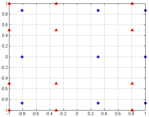
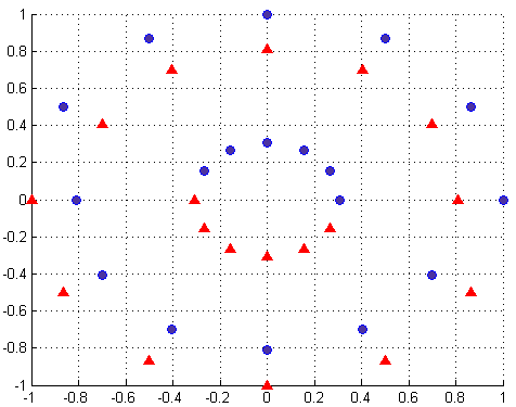
Figure 1: Left: Padua points for $n=5$ on the $(r,z)$-plane. We used different markers for the two Chebsyhev meshes of Padua points. Right: Projections on the disk of WAM2 points (obtained by $n+1$ rotations of Padua points around the $z$ axis). Notice that the points indicated with the small triangles are on different levels. See also Figure [Fig1].

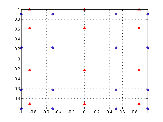
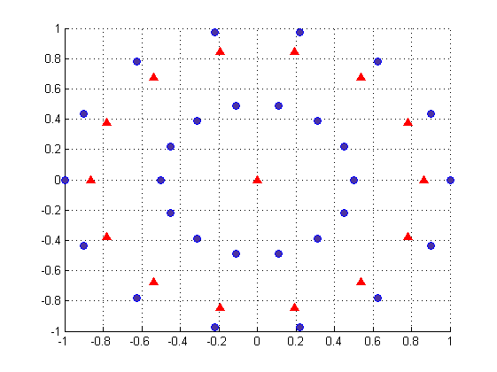
Figure 2: Left: Padua points for $n=6$ on the $(r,z)$-plane. We used different markers for the two Chebsyhev meshes of Padua points. Right: Projections on the disk of WAM2 points (obtained by $n+1$ rotations of Padua points around the $z$ axis). Notice that the points indicated with the small triangles are on a different levels.

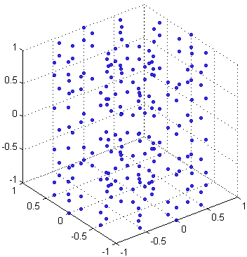
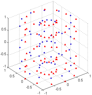
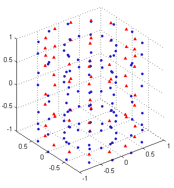
Figure 3: Above: the first WAM for $n=5$ having $216$ points. Below left: the second WAM for $n=5$ having $126$ points. Below right: the second WAM for $n=6$ having $172$ points.

3 Computation of AFP and DLP

As discussed in [4], the computation the AFP and DLP, can be done by a few basic linear algebra operations, corresponding to the LU factorization with row pivoting of the Vandermonde matrix for the DLP, and to the QR factorization with column pivoting of the transposed Vandermonde matrix for the AFP (cf. [15]). For the sake of completeness, we recall these two Matlab-like scripts used in [15, 4] for computing the AFP and DLP, respectively. algorithm AFP (Approximate Fekete Points):
$\bullet$ $W=(V(\boldsymbol{a},\boldsymbol{p}))^{t}$; $\boldsymbol{b}=(1,\dots,1)^{t}\in\mathbb{C}^{N}$; $\boldsymbol{w}=W\backslash\boldsymbol{b}\,$; $ind=\mbox{{find}}(\boldsymbol{w}\neq\boldsymbol{0})$; $\boldsymbol{\xi}=\boldsymbol{a}(ind)$ algorithm DLP (Discrete Leja Points):
$\bullet$ $V=V(\boldsymbol{a},\boldsymbol{p})$; $[L,U,\boldsymbol{\sigma}]=\mbox{{LU}}(V,\mbox{``{vector}''})$; $ind=\boldsymbol{\sigma}(1,\dots,N)$; $\boldsymbol{\xi}=\boldsymbol{a}(ind)$

In Figures 4–5, we show the AFP and DLP extracted from the WAM1 and WAM2 for $n=5$. In the above scripts, $V(\boldsymbol{a},\boldsymbol{p})$ indicates the Vandermonde matrix at the WAM $\boldsymbol{a}$ using the polynomial basis $\boldsymbol{p}$, that is the matrix whose elements are $p_{j}(a_{i}),\;1\leq j\leq N,\;1\leq i\leq{\tt card}(A_{n})$. The extracted AFP and DLP are then stored in the vector $\boldsymbol{\xi}$. Remark 1. In both algorithms, the selected points (as opposed to the continuum Fekete points) depend on the choice of the polynomial basis. But in the second algorithm, which is based on the notion of determinant (as described in [4, §6.1]), the selected points also depend on the ordering of the basis. In the univariate case with the standard monomial basis, it is not difficult to recognize that the selected points are indeed the Leja points extracted from the mesh (cf. [1, 14] and references therein). Remark 2. When the conditioning of the Vandermonde matrices is too high, and this happens when the polynomial basis is ill-conditioned, the algorithms can still be used provided that a preliminary iterated orthogonalization, that is a change to a discrete orthogonal basis, is performed (cf. [3, 4, 15]). This procedure however only mitigates the effect of a bad choice of the polynomial basis. Consequently, whenever is possible, is desirable to use a well-conditioned polynomial basis.

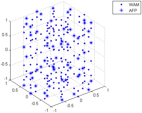
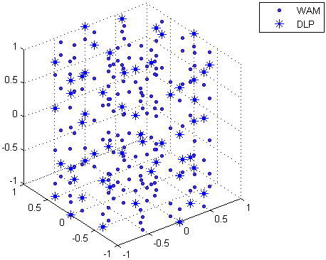
Figure 4: WAM1 of the cylinder for $n=5$ and the corresponding extracted points. Left: $56$ Approximate Fekete Points. Right: $56$ Discrete Leja Points.

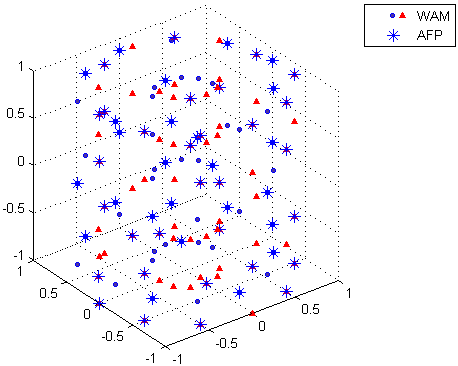
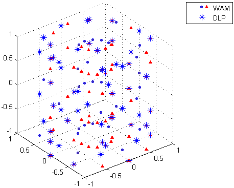
Figure 5: WAM2 of the cylinder for $n=5$ and the corresponding extracted points. Left: $56$ Approximate Fekete Points. Right: $56$ Discrete Leja Points.

A suitable basis for the forementioned rectangular cylinder $K$, is the set of polynomials introduced by J. Wade in [18]:

$$C_{j,k,i}(x,y,z):=U_{k}(\theta_{j,k};x,y)\tilde{T}_{i-k}(z),\;\;i=0,\ldots,n,\,\,k=0,\ldots,i,\,\,j=0,\ldots,k$$ (3.8)

where

• $\theta_{j,k}=\frac{j\pi}{k+1}$;

• $U_{k}(\theta_{j,k};x,y)=U_{k}(x\cos(\theta_{j,k})+y\sin(\theta_{j,k}))$ is the Chebyshev polynomial of the second kind which is an orthonormal basis for the disk w.r.t. the measure $\omega(x,y)=\frac{1}{\pi}$;

• $\tilde{T}_{j}(z)$ is the $j$-th orthonormal Chebyshev polynomial of the first kind, i.e. $\tilde{T}_{j}(z)=\sqrt{2}T_{j}(z)$, w.r.t. the measure $\omega(z)=(1-z^{2})^{-\frac{1}{2}}$.

As discussed in [18], the basis $C_{j,k,i}(x,y,z)$ is orthonormal for the space of orthogonal polynomials on $K$ w.r.t. the weight function $\frac{1}{\pi}{(1-z^{2})}^{-\frac{1}{2}}$. This basis plays also an important role in the construction of the discretized Fourier orthogonal expansions on the disk $D$ and the unitary rectangular cylinder. Moreover, this turns out to be well-conditioned. Indeed, as outlined in [18], if we consider the Radon projection of a function $f$ on $\mathbb{R}^{d}$

$$R_{\theta}(f;t)=\int_{<x,\theta>=t}f(x)dx,\;\;t\in\mathbb{R},\;\theta\in\mathbb{S}^{d-1}$$

with $\mathbb{S}^{d-1}$ the unit sphere in $\mathbb{R}^{d}$. The discretized Fourier expansion $F_{2m}$ of $R_{\theta}(f;t)$ for $m\geq 0$, $(x,y)$ belonging to the unit disk and $z\in[-1,1]$

$$F_{2m}(f)(x,y,z)=\sum_{i=0}^{2m}\sum_{j=1}^{2m}\sum_{k=0}^{2m-1}R_{\phi_{\nu}}(f(\cdot,\cdot,z_{k,2m};\cos(\theta_{j,2m}))){\cal T}_{i,j,k}(x,y,z)$$

where $\phi_{\nu}={2\nu\pi\over 2m+1}$,

$${\cal T}_{i,j,k}(x,y,z)={1\over 4m^{2}(2m+1)}\sum_{n=0}^{2m}\sum_{l=0}^{n}(l+1)\sin((l+1)\theta_{j,2m})U_{l}(\cos(\sigma_{i}(x,y)))T_{n-l}(z_{k,2m})T_{n-l}(z)$$

and $\sigma_{i}(x,y)=\arccos(x\cos\phi_{i}+y\sin\phi_{i})$, has sup norm that grows as $\|F_{2m}\|_{\infty}\approx m(\log(m+1)^{2})$, i.e. nearly the optimal growth.

4 Approximation and cubature on the cylinder

4.1 Interpolation and least-square approximation

The interpolation polynomial $q_{n}({\bf x})$ of degree $n$ of a real continuous function $f$ defined on the compact $K\subset\mathbb{R}^{3}$, can be written in Lagrange form as

$$q_{n}({\bf x})=\sum_{j=1}^{N}f({\bf a}_{j})l_{j}({\bf x}),\;{\bf x}\in K$$ (4.9)

where $N={\tt dim}(\mathbb{P}_{n}^{3})$, ${\bf a}_{j}$ are the AFP or the DLP extracted from the WAMs and $l_{j}$ indicates the $j$th elementary Lagrange polynomial of degree $n$. Let ${\bf l}=(l_{1}({\bf x}),\ldots,l_{N}({\bf x}))$ be the (row) vector of all the elementary Lagrange polynomials at a point ${\bf x}$, ${\bf p}$ the vector of the basis (3.8) and ${\bf a}=({\bf a}_{1},\ldots,{\bf a}_{N})$, then we can compute ${\bf l}$ by solving the linear system

$${\bf l}^{t}=W\,{\bf p}^{t},\;\;W=(V({\bf a},{\bf p})^{-1})^{t}\,.$$

The interpolation operator ${\cal L}_{n}:{\cal C}(K)\rightarrow\mathbb{P}^{3}_{n}$, with ${\cal C}(K)$ equipped with the sup norm, that maps every $f\in{\cal C}(K)$ into the corresponding polynomial $q=\sum_{i=1}^{N}l_{i}(\cdot)f({\bf x}_{i})\in\mathbb{P}^{3}_{n}$ in Lagrange form, is a projection having norm

$$\|{\cal L}_{n}\|_{\infty}=\max_{{\bf x}\in K}\sum_{j=1}^{N}|l_{j}({\bf x})|:=\Lambda_{n}$$ (4.10)

where $\Lambda_{n}$ is the well-known Lebesgue constant. When the interpolation points are the true Fekete points, the Lebesgue constant satisfies the upper bound

$$\Lambda_{n}=\max_{{\bf x}\in K}\|W\,{\bf p}^{t}\|_{1}\leq N\,$$

since $\|l_{j}\|\leq 1$.

Thanks to property P10 of WAMs we can say more. Indeed, when the Fekete points are extracted from a WAM, $\|l_{j}\|_{K}\leq C(A_{n})\|l_{j}\|_{A_{n}}\;\forall j$ (cf. [8, §4.4]), from which the following upper bound holds

$$\Lambda_{n}\leq N\,C(A_{n})\,,$$

with $C(A_{n})$, the same constant in definition of a WAM, which depends on $A_{n}$. In the numerical experiments that we will present in the next section, we will observe that the above upper bound is a quite pessimistic overestimate. Another natural application of such a construction, is the least squares approximation of a function $f\in{\cal C}(K)$. Given a WAM $A_{n}=\{{\bf a}_{1},\ldots,{\bf a}_{M}\},\,M\geq N$, with $N=\mbox{dim}(\mathbb{P}_{n}^{3})$ and ${\bf p}=\{p_{1},\ldots,p_{N}\}$ a basis for $\mathbb{P}_{n}^{3}$, let us consider the orthonormal basis ${\bf q}$ w.r.t. the discrete inner product $\left<f,g\right>=\sum_{i=1}^{M}f({\bf a}_{i})\overline{g({\bf a}_{i})}$ which can be obtained from the basis ${\bf p}$ by multiplying by a certain transformation matrix $P$, i.e. q=Pp.

The least squares operator of $f$ at the points of a WAM $A_{n}$ can then be written as

$${L}_{A_{n}}(f)({\bf x})=\sum_{j=1}^{N}\left(\sum_{i=1}^{M}f({\bf a}_{i})\overline{q_{j}({\bf a}_{i})}\right)q_{j}({\bf x})=\sum_{i=1}^{M}f({\bf a}_{i})g_{i}({\bf x})$$

where $g_{i}({\bf x})=\sum_{j=1}^{N}q_{j}({\bf x})\overline{q_{j}({\bf a}_{i})}$. Letting ${\bf g}=(g_{1},\ldots,g_{M})^{t}$, it follows that ${\bf g}=QP^{t}{\bf p}$, where the matrix $Q$ is a numerically orthogonal (unitary) matrix, i.e. $\bar{Q^{t}}Q=I$, and $Q=V({\bf a},{\bf q})=V({\bf a},{\bf p})P$. Notice that, the transformation matrix $P$ and the matrix $Q$ are computed once and for all for a fixed mesh.

The norm of the operator, that is its Lebesgue constant, is then

$$\|{L}_{A_{n}}\|=\max_{{\bf x}\in K}\sum_{i=1}^{M}|g_{i}({\bf x})|=\max_{{\bf x}\in K}\|QP^{t}{\bf p}({\bf x})\|_{1}\,.$$

In [8], it is observed that three-dimensional WAMs so defined can be used as discretization of compact sets $K\subset\mathbb{R}^{3}$ for the computation of good points for least-square approximation by polynomials. Indeed, using property P9, in [8, Th. 2] the authors proved the following error estimates for least-squares approximation on WAMs of a function $f\in{\cal C}(K)$

$$\|f-L_{A_{n}}(f)\|_{K}\leq\left(1+C(A_{n})(1+\sqrt{{\tt card}(A_{n})})\right)\min\{\|f-p\|_{K}\,:\,p\in\mathbb{P}_{n}^{3}\}$$ (4.11)

where again $C(A_{n})$ depends on the WAM.

This estimates says that if we could control the factor $C(A_{n})(1+\sqrt{{\tt card}(A_{n})})$, and this is possible when we use WAMs, then the approximation $L_{A_{n}}(f)\in\mathbb{P}_{n}^{3}$ is nearly optimal.

4.2 Cubature

For a given function $f:K\subset\mathbb{R}^{3}\rightarrow\mathbb{R}$ we want to compute

$$I(f)=\int_{K}f({\bf x})d{\bf x}$$

where $d{\bf x}$ is the usual Lebesgue measure of the compact set $K$. An interpolating cubature formula $C_{N}(f)$ that approximates $I(f)$ can be expressed as

$$C_{N}(f)=\sum_{i=1}^{N}w_{i}f({\bf x}_{i})\,$$

where, in our case, the nodes ${\bf x}_{i}$ are the AFP or the DLP for $K$. Once we know the cubature weights $w_{i}$, the $C_{N}(f)$ gives an approximation of $I(f)$. The cubature weights can be determined by solving the moment system, that is

$$\sum_{j=1}^{N}w_{j}p_{i}({\bf x}_{j})=\int_{K}p_{i}({\bf x})d{\bf x},\;\;i=1,\ldots,N$$

where $p_{i}$ is the $i$-th element of the polynomial basis p. Hence, if $V=(p_{i}(x_{j}))$ and $b_{i}=\int_{K}p_{i}(x)dx$, the nodes $x_{i}$ and the weights $w_{i}$ are provided by the AFP or DLP algorithm.

5 Numerical results

In this section we present the numerical experiments that we made for showing the quality of AFP and DLP on interpolation, approximation by least-squares and cubature of $6$ test functions defined on the rectangular cylinder $K=D\times[-1,1]$. The results are obtained by using both the AFP and the DLP extracted from both WAM1 and WAM2.

In Table 1 we collect, for degrees $n=5,10,15,20,25,30$, the values of the Lebesgue constant $\Lambda_{n}$, those of the condition number (in the sup norm) $\kappa_{\infty,1}$ for the associated Vandermonde matrix using the Wade basis for the WAM1 for the AFP. Due to hardware restrictions, the Lebesgue constant has been evaluated on a control mesh $M_{n}=A_{m}$ with $m=4n$ for $n\leq 20$, $m=2n$ for $n>20$.

In Table 2 we present $\Lambda_{n},\,\kappa_{\infty,2}$ for the WAM2 on the AFP. In this case the control mesh $M_{n}=A_{m}$ with $m=4n$ for $n\leq 20$, $m=3n$ for $n\leq 25$ and $m=2n$ for $n>25$.

In Tables 3 and 4 we present the corresponding values for the DLP.

In Table 5 we display the the norm of the least-square operator $\|L_{A_{n}}\|$ on the WAM1 and WAM2, respectively.

Note that the norm of the least-square operator $\|L_{A_{n}}\|$ (norm computed at the points of the WAM $A_{n}$) has been computed after two steps of orthonormalization of the polynomial basis.

The numerical results show that both $\Lambda_{n}$ and the condition number $\kappa_{\infty,*}$ are smaller for WAM2 while, by oppositeon the contrary, the sup norm of the least-square operator turns out to be bigger for WAM2 than WAM1. Actually, for WAM2, $\|L_{A_{n}}\|$ has a growth factor close to $2$.

n	5	10	15	20	25	30
$\Lambda_{n}$	17	83	208	384	849	988
$\kappa_{\infty,1}$	18.2	177	384	746	1410	2650

Table 1: The Lebesgue constant and the condition number of the Vandermonde matrix constructed using the Wade basis on the AFP for the WAM1.

n	5	10	15	20	25	30
$\Lambda_{n}$	19	76	213	427	879	1034
$\kappa_{\infty,2}$	19.4	115	440	705	1540	2380

Table 2: The Lebesgue constant and the condition number of the Vandermonde matrix constructed using the Wade basis on the AFP for the WAM2.

n	5	10	15	20	25	30
$\Lambda_{n}$	30	115	350	617	1388	2597
$\kappa_{\infty,1}$	35.2	247	772	1190	3090	5320

Table 3: The Lebesgue constant and the condition number of the Vandermonde matrix constructed using the Wade basis on the DLP for the WAM1.

n	5	10	15	20	25	30
$\Lambda_{n}$	30	129	349	648	1520	2143
$\kappa_{\infty,2}$	29.9	176	638	782	2310	3940

Table 4: The Lebesgue constant and the condition number of the Vandermonde matrix constructed using the Wade basis on the DLP for the WAM2.

n	5	10	15	20	25	30
$||{L}_{A_{n,1}}||$	4.8	10.2	10.7	21.1	15.8	22.6
$||{L}_{A_{n,2}}||$	7.2	15.3	32.8	43.4	85.9	96.6

Table 5: The sup-norm of the least-squares operator on WAM1 and WAM2, respectively.

The interpolation and the cubature relative errors on the AFP and the DLP have been computed for the following six test functions:

$$f_{1}(x,y,z) = 0.75{\tt e}^{-\frac{(9x-2)^{2}+(9y-2)^{2}+(9z-2)^{2}}{4}}+0.75{\tt e}^{-\frac{(9x+1)^{2}}{49}-\frac{9y+1}{10}-\frac{9z+1}{10}}$$

$$+ 0.5{\tt e}^{-\frac{(9x-7)^{2}+(9y-3)^{2}+(9z-5)^{2}}{4}}-0.2{\tt e}^{-(9x-4)^{2}-(9y-7)^{2}-(9z-5)^{2}};$$

$$f_{2}(x,y,z) = \sqrt{(x-0.4)^{2}+(y-0.4)^{2}+(z-0.4)^{2}};$$

$$f_{3}(x,y,z) = \cos(4(x+y+z));$$

$$f_{4}(x,y,z) = \frac{1}{1+16(x^{2}+y^{2}+z^{2})};$$

$$f_{5}(x,y,z) = \sqrt{(x^{2}+y^{2}+z^{2})^{3}};$$

$$f_{6}(x,y,z) = \cos(x^{2}+y^{2}+z^{2})\,.$$

The function $f_{1}$ is the three-dimensional equivalent of the well-known Franke test function. The function $f_{2}$ has a singular point into the cylinder $K=D\times[-1,1]$. The functions $f_{3}$ and $f_{6}$ are infinitely differentiable. The function $f_{4}$ is the Runge function. The function $f_{5}$ is a ${\cal C}^{2}$ function with third derivatives singular at the origin.

All numerical experiments have been done on a cluster HP with 14 nodes. We used one of the nodes equipped with 2 processors quad core with 64Gb of RAM.

In Figures 6 and 7 we display the interpolation, cubature and least-square relative errors on the AFP and DLP, up to degree $n=30$, for the WAM1 and WAM2, respectively. The results shows that the AFP give, in general, smaller errors. Only the cubature errors on WAM2 are smaller for DLP than AFP. One reason is related to the values of the Lebesgue constants and the conditioning of the Vandermonde matrices that are smaller for AFP than DLP.

Since WAM2 has a lower cardinality and that the results are more or less the same, such a mesh is more convenient from the point of view of efficiency and approximation order. As true values of the functions $f_{i},\;i=1,\ldots,6$, we considered the value of $f_{i}$ on the control meshes used for computing the Lebesgue constants. As exact values of the integrals, we considered the values computed by the Matlab built-in function triplequad with the chosen tolerance depending on the smoothness of the function. For the smoothest functions $f_{3}$ and $f_{6}$ we used the tolerance $1.e-12$ while for the others $1.e-10$. This choice allowed to avoid stalling phenomena that we encountered in computing the integrals of $f_{3}$ and $f_{6}$.

We point out that in the case of the function $f_{2}$, where there exist a singularity in $(0.4,0.4,0.4)$, triplequad uses a domain decomposition approach, implemented in the method quadgk (Gauss-Kronrod cubature rules) avoiding the singularity. Actually, due to the geometry of the cylinder, we could compute the exact values for the integrals by using separation of variables, that is instead of a call to the Matlab built-in function triplequad we used the product of the built-in functions dblquad and quadl. This allowed a considerably reduction of the computational time, as displayed in Table 6 for degrees $n\leq 20$.

Concerning function $f_{4}$, the least-square errors seem not those that one can expected. In [7, Fig. 3.2] the authors already computed the relative hyperinterpolation errors for the Runge function w.r.t. the number of function evaluations. From that figure, correspondingly to polynomial degree $n=30$, that requires $(n+1)(n+2)(n+3)/6=5456$ function evaluations, the hyperinterpolation error is about $10^{-1}$. Hence, what we see in Figure 7 is consistent with those results and, as expected, formula (4.11) is an overestimate of the least-square error.

n	triplequad	dblquad$\times$quadl
5	1 min. 9 sec.	4.7 sec.
10	16 min. 3 sec.	1 min. 4 sec.
15	1 h 15 min. 10 sec.	5 min. 33 sec.
20	3 h 47 min. 12 sec.	16 min. 30 sec.

Table 6: Computational time: triplequad vs doublequad$\times$quadl

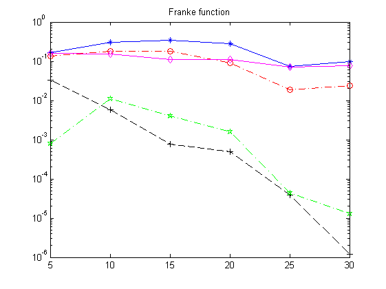
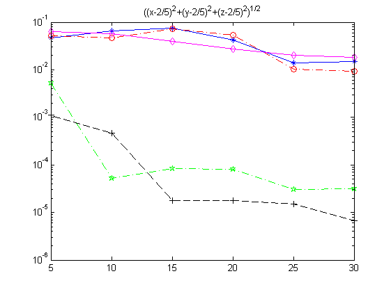
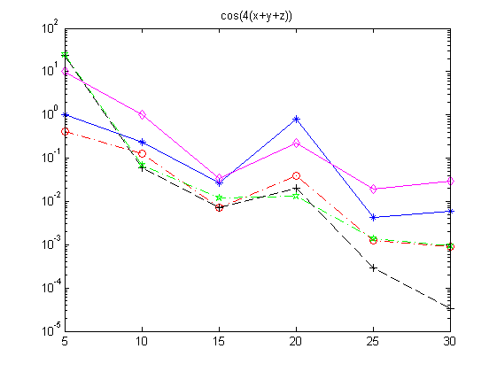
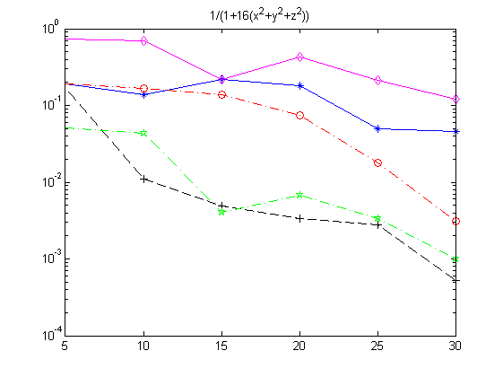
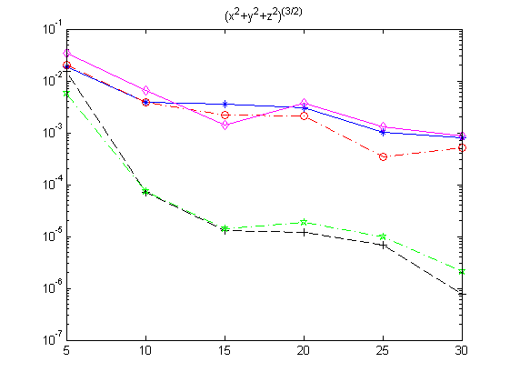
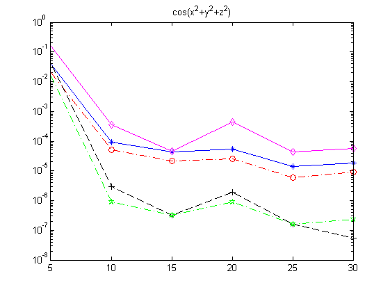
Figure 6: Interpolation error on AFP (blue $-*$), cubature errors on AFP (black $-+$) Interpolation error on DLP (magenta $-\diamond$), cubature errors on DLP (green $--\star$) and least-squares errors (red $-\cdot$o). The points are extracted from the WAM1. Wade basis. In abscissa the polynomial degree.

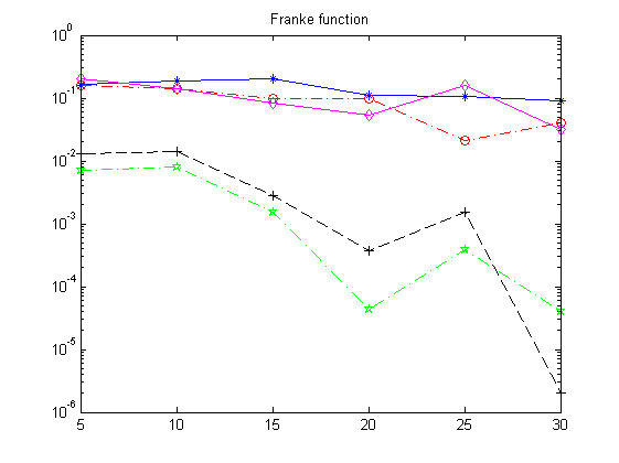
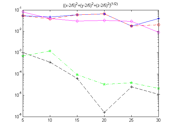
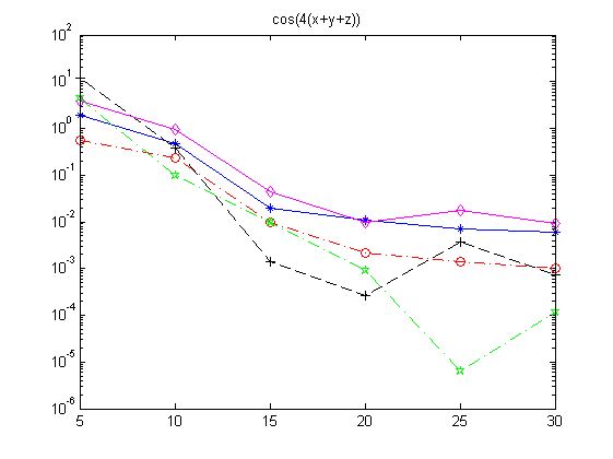
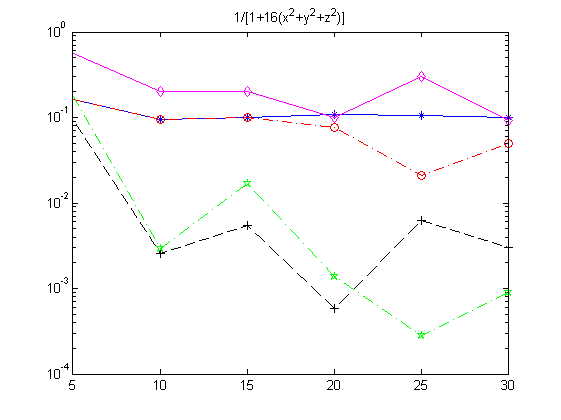
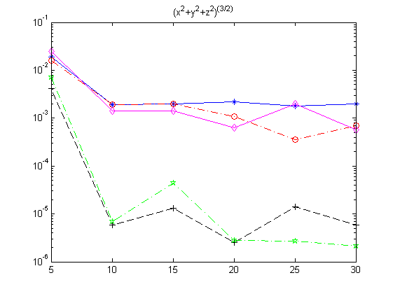
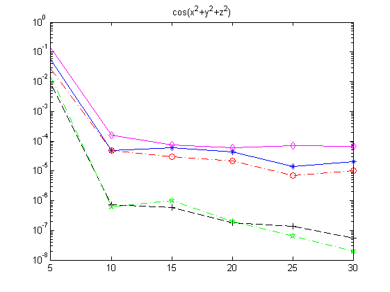
Figure 7: Interpolation error on AFP (blue $-*$), cubature errors on AFP (black $-+$) Interpolation error on DLP (magenta $-\diamond$), cubature errors on DLP (green $--\star$) and least-squares errors (red $-\cdot$o). The points are extracted from the WAM2. Wade basis. In abscissa the polynomial degree.

Acknowledgments. This work has been done with the support of the 60% funds, year 2010 of the University of Padua.

References

- [1] L. Bialas-Cieź and J.-P. Calvi, Pseudo Leja sequences, Ann. Mat. Pura Appl., published online November 16, 2010.
- [2] L. Bos, M. Caliari, S. De Marchi, M. Vianello and Y. Xu, Bivariate Lagrange interpolation at the Padua points: the generating curve approach, J. Approx. Theory 143 (2006), 15–25.
- [3] L. Bos, J.-P. Calvi, N. Levenberg, A. Sommariva and M. Vianello, Geometric weakly admissible meshes, discrete least squares approximation and approximate Fekete points, to appear in Math. Comp. (2010) (preprint online at: http://www.math.unipd.it/marcov/CAApubl.html).
- [4] L. Bos, S. De Marchi, A. Sommariva and M. Vianello, Computing multivariate Fekete and Leja points by numerical linear algebra, SIAM J. Numer. Anal. 48 (2010), 1984–1999.
- [5] L. Bos, S. De Marchi, A. Sommariva and M. Vianello, Weakly Admissible Meshes and Discrete Extremal Sets, Numer. Math. Theory Methods Appl. 4 (2011), 1–12.
- [6] L. Bos, A. Sommariva and M. Vianello, Least-squares polynomial approximation on weakly admissible meshes: disk and triangle, J. Comput. Appl. Math. 235 (2010), 660–668.
- [7] S. De Marchi, M. Vianello and Y. Xu, New cubature formulae and hyperinterpolation in three variables, BIT, Vol. 49(1) 2009, 55-73.
- [8] J. P. Calvi and N. Levenberg, Uniform approximation by discrete least squares polynomials, J. Approx. Theory 152 (2008), 82–100.
- [9] A. Civril and M. Magdon-Ismail, On selecting a maximum volume sub-matrix of a matrix and related problems, Theoretical Computer Science 410 (2009), 4801–4811.
- [10] M. Klimek, Pluripotential Theory, Oxford U. Press, 1992.
- [11] A. Kroó, On optimal polynomial meshes, J. Approx. Theory, to appear.
- [12] M. Marchioro, Punti di Approssimati di Fekete e Discreti di Leja del parallelepipedo, del cilindro e del prisma retto, Master Thesis, University of Padua (2010) (in Italian).
- [13] F. Piazzon and M. Vianello, Analytic transformations of admissible meshes, East J. Approx. 16 (2010), 313–322.
- [14] E.B. Saff and V. Totik, Logarithmic potentials with external fields, Springer, 1997.
- [15] A. Sommariva and M. Vianello, Computing approximate Fekete points by QR factorizations of Vandermonde matrices, Comput. Math. Appl. 57 (2009), 1324–1336.
- [16] A. Sommariva and M. Vianello, Gauss-Green cubature and moment computation over arbitrary geometries, J. Comput. Appl. Math. 231 (2009), 886–896.
- [17] A. Sommariva and M. Vianello, Approximate Fekete points for weighted polynomial interpolation, Electron. Trans. Numer. Anal. 37 (2010), 1–22.
- [18] J. Wade, A discretized Fourier orthogonal expansion in orthogonal polynomials on a cylinder, J. Approx. Theory 162 (2010), 1545–1576.