Goodness-of-fit tests for weibull populations on the basis of records

Abstract

Record is used to reduce the time and cost of running experiments (Doostparast and Balakrishnan, 2010). It is important to check the adequacy of models upon which inferences or actions are based (Lawless, 2003, Chapter 10, p. 465). In the area of goodness of fit based on record data, there are a few works. Smith (1988) proposed a form of residual for testing some parametric models. But in most cases, the variation inherent in graphical summaries is substantial, even when the data are generated by assumed model, and the eye can not always determine whether features in a plot are within the bounds of natural random variation. Consequently, formal hypothesis tests are an important part of model checking (Lawless, 2003).
In this paper, Kolmogorov-Smirnov and Cramer-von Mises type goodness of fit tests for record data are proposed. Also a new weighted goodness of fit test is suggested. A Monte-Carlo simulation study is conducted to derive the percentiles of the statistics proposed. Finally, some real data sets are given to investigate results obtained.

Key Words: Cramer-von Mises Statistics; Exponential model; Goodness of fit test; Kolmogorov-Smirnov statistics; Likelihood ratio test; Record data; Weibull model.

1 Introduction

In reliability, we are concerned primarily with test data in which lifetimes of items that fail during the course of the test are recorded or with variables related in some way to item lifetimes. If the actual lifetime of every item in the sample is recorded, the data are complete data. To obtain complete data, it is necessary to continue the experiment until the last item on test or in service has failed. In cases where even a few items in the sample may have very long lifetimes, experiment can go on for a very long period of time and, in fact, well beyond the point at which the results may no longer be of any interest or use. In such situations, it may be desirable to terminate the study prior to failure of all items under test. When observation is discontinued prior to all items having failed, we obtain the so-called censored data. There are a variety of forms of censored data that arise in practice; See, for example, Balakrishnan and Cohen (1991) and Cohen (1991).

A form of censored data that is often encountered in applications is the so-called record data. As pointed out by Gulati and Padgett (1995), often, in industrial testing, meteorological data, and some other situations, measurements may be made sequentially and only values smaller (or larger) than all previous ones are recorded. Such data may be represented by $(\textbf{r,k}):=(r_{1},k_{1},r_{2},k_{2},\cdots,r_{m},k_{m})$, where $r_{i}$ is the $i$-th record value meaning new minimum (or maximum) and $k_{i}$ is the number of trials following the observation of $r_{i}$ that are needed to obtain a new record value (or to exhaust the available observation). There are two sampling schemes for generating such a record-breaking data:

• (Inverse sampling scheme) Items are presented sequentially and sampling is terminated when the $m$-th minimum is observed. In this case, the total number of items sampled is a random number, and $K_{m}$ is defined to be one for convenience;

• (Random sampling scheme) A random sample $Y_{1},\cdots,Y_{n}$ is examined sequentially and successive minimum values are recorded. In this setting, we have $N^{(n)}$, the number of records obtained, to be random and, given a value of $m$, we have in this case $\sum_{i=1}^{m}K_{i}=n$.

A random variable $X$ is said to have an exponential distribution, denoted by $X\sim Exp(\sigma)$, if its cumulative distribution function (cdf) is

$$F(x;\sigma)=1-\exp\left\{-\left(\frac{x}{\sigma}\right)\right\},\ \ \ x\geq 0,\ \ \ \sigma>0,$$ (1)

and the probability density function (pdf) is

$$f(x;\sigma)=\frac{1}{\sigma}\exp\left\{-\left(\frac{x}{\sigma}\right)\right\},\ \ \ x\geq 0,\ \ \ \sigma>0.$$ (2)

The exponential distribution is commonly used in many applied problems. Such a exponential distribution is a natural model while studying a variable that can take on only positive values such as lifetime of units. In some situations, the Weibull distribution is more suitable than the exponential distributions (Nelson, 1985). The Weibull cdf, denoted by $W(\alpha,\sigma)$, is

$$F(x;\alpha,\sigma)=1-\exp\left\{-\left(\frac{x}{\sigma}\right)^{\alpha}\right\},\ \ \ \alpha>0,\ \ \sigma>0,$$ (3)

and hence with pdf

$$f(x;\alpha,\sigma)=\frac{\alpha x^{\alpha-1}}{\sigma^{\alpha}}\exp\left\{-\left(\frac{x}{\sigma}\right)^{\alpha}\right\},\ \ \ \alpha>0,\ \ \sigma>0.$$ (4)

The scale parameter $\sigma$ is called the characteristic life because it is always 63.2-th percentile. It determines the spread and has the same units as failure times, for example hours, months, cycles, and so forth. Parameter $\alpha$ is a unitless pure number and determines the shape of the distribution. For $\alpha=1$, the Weibull distribution is the exponential distribution. The Weibull distribution appears very frequent in practical problems when we observe data representing minimal values. For example, the life of a capacitor is determined by shortest-lived portion of dielectric. For many parent populations with limited left tail, the limit of the minimum of independent samples converges to a Weibull distribution (Lawless, 2003). Researchers often like to make parametric assumptions on the underlying distribution. With this in mind, estimation of the mean of an exponential distribution based on record data has been treated by Samaniego and Whitaker (1986) and Doostparast (2009). Hoinkes and Padgett (1994) obtained the ML estimators from record-breaking data in this model.

As pointed out by Lawless (2003, Chapter 10, p. 465), it is important to check the adequacy of models upon which inferences or actions are based. In the area of goodness of fit based on record data, there is a lack of published literature. But, there are a few works in this direction. However, informal methods of model checking emphasize graphical procedures such as probability and residual plots, Smith (1988) proposed a form of residual for testing some parametric models. But in most cases, the variation inherent in graphical summaries is substantial, even when the data are generated by assumed model, and the eye can not always determine whether features in a plot are within the bounds of natural random variation. Consequently, formal hypothesis tests are an important part of model checking.

Motivated by this, the aim of this paper is to provide some methods for model checking on the basis of records. Specifically, suppose that the record data $\{R_{1},K_{1},\cdots,R_{m},K_{m}\}$ are coming from a population with parent cdf $F(.)$. We consider testing

$$H_{0}:F(x)=1-\exp\left\{-\left(\frac{x}{\sigma}\right)^{\alpha}\right\},\ \ \ \forall\ \ x\in(0,+\infty).$$ (5)

where $\alpha$ and $\sigma$ may be unknown positive constants. In other word, is the weibull model adequate to fit the data? Therefore, the rest of this article is organized as follows. Since weibull model has a wide variety application, in Section 2, maximum likelihood estimate (MLE) of the unknown parameters in Weibull model are obtained. In Section 3, explicit expression for Kolmogorov-Smirnov (K-S) and Cramer-Misses (C-M) goodness of fit tests is derived and we proposed a new modified goodness of fit test which is more suitable than the K-S and C-M statistics for records. Critical values of these statistics are obtained by a simulation study. In Section 4, Exponential model is considered and goodness of fit test for exponential model against the alternative weibull model is obtained. Finally, some numerical examples are given to investigate results obtained.

2 Fitting a Weibull model

It can be shown that, the likelihood function for the two sampling schemes is given by

$$L(\theta)\equiv\prod_{i=1}^{m}f(r_{i})\left\{1-F(r_{i})\right\}^{k_{i}-1},\ \ \ 0<r_{m}<\cdots<r_{2}<r_{1}.$$ (6)

Let us assume that the sequence $\{R_{1},K_{1},\cdots,R_{m},K_{m}\}$ are coming from $W(\alpha,\sigma)$-model. The corresponding likelihood function under either random or inversely sampling is obtained as

$$L(\theta)\equiv\frac{\alpha^{m}}{\sigma^{m\alpha}}\left\{\prod_{i=1}^{m}r_{i}\right\}^{\alpha-1}\exp\left\{-\frac{1}{\sigma^{\alpha}}\sum_{i=1}^{m}k_{i}r_{i}^{\alpha}\right\}.$$ (7)

After taking logarithm, we have

$$l(\theta)\equiv m\log(\alpha)-m\alpha\log(\sigma)+(\alpha-1)\sum_{i=1}^{m}\log(r_{i})-\frac{1}{\sigma^{\alpha}}\sum_{i=1}^{m}k_{i}r_{i}^{\alpha}.$$ (8)

Through this paper ”log” denotes natural logarithm. One can easily show that, the maximum of (8) for $m\geq 2$, by taking derivatives, is obtained from solving the equations

$$\sigma=\left\{\frac{1}{m}\sum_{i=1}^{m}k_{i}r_{i}^{\alpha}\right\}^{1/\alpha},$$ (9)

and

$$h(\alpha)=\frac{1}{m}\sum_{i=1}^{m}\ln r_{i},$$ (10)

where

$$h(\alpha)=\frac{\sum_{i=1}^{m}k_{i}r_{i}^{\alpha}\ln r_{i}}{\sum_{i=1}^{m}k_{i}r_{i}^{\alpha}}-\frac{1}{\alpha}.$$

The equation (10) cannot be solved explicitly and hence the MLEs must be found by numerical methods. These equations is similar with equations (6.2) and (6.3) of Lehmann and Casella (1998, Ch. 6, p. 468). Hence, one can show that these equations have a unique solution.

3 GOF for weibull model

GOF tests can be based on the approaches of comparison of parametric estimates with nonparametric counterparts. Two well known examples are the Kolmogorov-Smirnov (K-S) and the Cramer-von Mises (C-M) statistics defined by

$$\hat{D}_{n}=\sup_{-\infty<x<+\infty}|\hat{F}(x)-F_{0}(x)|,$$ (11)

and

$$\hat{W}_{n}^{2}=n\int_{-\infty}^{+\infty}\left\{\hat{F}(x)-F_{0}(x)\right\}^{2}dF_{0}(x),$$ (12)

respectively, where $F_{0}(x)$ is the hypothesized model while $\hat{F}(x)$ is the corresponding nonparametric maximum likelihood estimation (NPMLE). On the basis of record data, arising from a random sample with size $n$, Samaniego and Whitaker (1988) obtained NPMLE of survival function $\bar{F}(x):=1-F(x)$ as

$$\hat{\bar{F}}(x)=\prod_{i:r_{(i)}\leq x}\frac{\sum_{j=i}^{m}k_{(j)}-1}{\sum_{j=i}^{m}k_{(j)}},$$ (13)

where $r_{(0)}\equiv 0$ and $r_{(1)}<r_{(2)}<\cdots<r_{(m)}$ are the observed record values, ordered from smallest to largest and $\{k_{(i)}\}$ are the induced order statistics corresponding to the ordered record values $\{r_{(i)}\}$ or $k_{(i)}=k_{m-i+1}$, $i=1,2,\cdots,m$. As mentioned by Samaniego and Whitaker (1988), NPMLE in (13) will perform poorly when estimating the right tail of the actual distribution, thus we suggest a new GOF statistic as follows

$$DS_{n}=n\int_{0}^{+\infty}\left(\hat{\bar{F}}(x)-\bar{F}_{0}(x)\right)^{2}\frac{1}{F_{0}(x)}dF_{0}(x).$$ (14)

The basic idea for $DS_{n}$ is similar with Anderson-Darling statistic and is to measure the distance between $\hat{F}(x)$ and $F_{0}(x)$ in left tail region of $F_{n}(x)$ better than C-M statistic in (12). One may notice that, on the basis of record data, the statistics $D_{n}$, $W_{n}^{2}$ and $DS_{n}$ are modified so that the supreme and integral are over the range $y\leq r_{1}$. Sufficiently large values of $D_{n}$, $W_{n}^{2}$ or $DS_{n}$ provide evidence against the hypothesized model. To calculate the test statistics, the following Proposition is helpful.

Proposition 3.1

Let $R_{1},K_{1},\cdots,R_{m},K_{m}$ be record data arising from a random sample with size $n$. Then the statistics $D_{n}$, $W_{n}^{2}$ and $DS_{n}$ are simplified as

$$D_{n} = \max_{1\leq i\leq n}\left\{\max\left\{\hat{\Phi}_{1}\cdots\hat{\Phi}_{i-1}-\hat{\bar{F}}_{0}(r_{(i)}),\hat{\bar{F}}_{0}(r_{(i)})-\hat{\Phi}_{1}\cdots\hat{\Phi}_{i}\right\}\right\},$$ (15)

$$W_{n}^{2} = \frac{n}{3}\sum_{i=1}^{m+1}\left\{\left[\hat{\Phi}_{1}\cdots\hat{\Phi}_{i-1}-\hat{\bar{F}}_{0}(r_{(i)})\right]^{3}-\left[\hat{\Phi}_{1}\cdots\hat{\Phi}_{i-1}-\hat{\bar{F}}_{0}(r_{(i-1)})\right]^{3}\right\},$$ (16)

and

$$DS_{n} = n\left[\sum_{i=1}^{m+1}\left\{\left[\hat{\Phi}_{1}\cdots\hat{\Phi}_{i-1}-1\right]^{2}\ln\hat{F}_{0}(r_{(i)})-\left[\hat{\Phi}_{1}\cdots\hat{\Phi}_{i-1}-1\right]^{2}\ln\hat{F}_{0}(r_{(i-1)})\right\},\right.$$ (17)

$$\left.+2\sum_{i=1}^{m+1}\left\{\left[\hat{\Phi}_{1}\cdots\hat{\Phi}_{i-1}-1\right]\hat{F}_{0}(r_{(i)})-\left[\hat{\Phi}_{1}\cdots\hat{\Phi}_{i-1}-1\right]\hat{F}_{0}(r_{(i-1)})\right\}+\frac{1}{2}\right],$$

respectively, where $r_{(0)}\equiv 0$, $x_{m+1}\equiv+\infty$ and for $i=1$, $\hat{\Phi}_{1}\cdots\hat{\Phi}_{i-1}=1$ and

$$\hat{\Phi}_{i}=\frac{\sum_{j=i}^{m}k_{(j)}-1}{\sum_{j=i}^{m}k_{(j)}},\ \ \ 1\leq i\leq m.$$

Proof Proof of (15) is clear. For (16), we have

$$W_{n}^{2} = n\int_{0}^{+\infty}\left\{\hat{F}_{n}(y)-F_{0}(y)\right\}^{2}dF_{0}(y)$$

$$= n\int_{0}^{+\infty}\left\{\hat{\bar{F}}_{n}(y)-\bar{F}_{0}(y)\right\}^{2}dF_{0}(y)$$

$$= n\sum_{i=1}^{m+1}\int_{r_{(i-1)}}^{r_{(i)}}\left\{\hat{\bar{F}}_{n}(y)-\bar{F}_{0}(y)\right\}^{2}dF_{0}(y)$$

$$= n\sum_{i=1}^{m+1}\int_{r_{(i-1)}}^{r_{(i)}}\left\{\hat{\Phi}_{1}\cdots\hat{\Phi}_{i-1}-\bar{F}_{0}(y)\right\}^{2}dF_{0}(y)$$

$$= n\sum_{i=1}^{m+1}\int_{F_{0}(r_{(i-1)})}^{F_{0}(r_{(i)})}\left\{\hat{\Phi}_{1}\cdots\hat{\Phi}_{i-1}-1+u\right\}^{2}du$$

$$= \frac{n}{3}\sum_{i=1}^{m+1}\left[\left\{\hat{\Phi}_{1}\cdots\hat{\Phi}_{i-1}-1+\hat{F}_{0}(r_{(i)})\right\}^{3}-\left\{\hat{\Phi}_{1}\cdots\hat{\Phi}_{i-1}-1+\hat{F}_{0}(r_{(i-1)})\right\}^{3}\right].$$

Similarly, one can show (17) and desired result follows. $\Box$

Proposition 3.2

Assuming $H_{0}:F_{0}(y)=1-\exp\left\{-(x/\sigma)^{\alpha}\right\}$ is true. Conditionally on $\{N^{(n)}\geq 2\}$, the distribution of $D_{n}$, $W_{n}^{2}$ and $DS_{n}$, on the basis of record data do not depend on $F_{0}(y)$.

Proof Suppose $\{N^{(n)}\geq 2\}$. Let $R_{i}^{\prime}\stackrel{{\scriptstyle D}}{{\equiv}}(R_{i}/\sigma)^{\alpha}$. Thus, $R_{1}^{\prime},K_{1},\cdots,R_{m}^{\prime},K_{m}$ are coming from a random sample with common distribution function $W(1,1)$. The ML estimates on the basis of $R_{1}^{\prime},K_{1},\cdots,R_{m}^{\prime},K_{m}$, denoted by $\hat{\alpha}^{\prime}$ and $\hat{\sigma}^{\prime}$, are obtained by solving (9) and (10) replacing $r_{i}$ with $r_{i}^{\prime}$. One can easily verify that $\hat{\alpha}=\alpha\hat{\alpha}^{\prime}$. This implies that

$$\hat{\sigma} = \left\{\frac{1}{m}\sum_{i=1}^{m}K_{i}R_{i}^{\hat{\alpha}}\right\}^{\frac{1}{\hat{\alpha}}}$$

$$= \left\{\frac{1}{m}\sum_{i=1}^{m}K_{i}(\sigma R_{i}^{\prime 1/\alpha})^{\hat{\alpha}}\right\}^{\frac{1}{\hat{\alpha}}}$$

$$= \sigma\left\{\frac{1}{m}\sum_{i=1}^{m}K_{i}(R_{i}^{\prime})^{\hat{\alpha}/\alpha}\right\}^{\frac{1}{\hat{\alpha}}}$$

$$= \sigma\left\{\frac{1}{m}\sum_{i=1}^{m}K_{i}(R_{i}^{\prime})^{\hat{\alpha}^{\prime}}\right\}^{\frac{1}{\hat{\alpha}^{\prime}\alpha}}$$

$$= \sigma\left\{\hat{\sigma}^{\prime}\right\}^{1/\alpha}.$$

Hence, the estimate of weibull distribution function is obtained as

$$\hat{F}_{0}(x;\alpha,\sigma) = F_{0}(x;\hat{\alpha},\hat{\sigma})$$ (18)

$$= 1-\exp\left\{-\left(\frac{x}{\hat{\sigma}}\right)^{\hat{\alpha}}\right\}$$

$$= 1-\exp\left\{-\left(\frac{x}{\sigma\left\{\hat{\sigma}^{\prime}\right\}^{1/\alpha}}\right)^{\alpha\hat{\alpha}^{\prime}}\right\}$$

$$= 1-\exp\left\{-\left(\left[\frac{x}{\sigma}\right]^{\alpha}\frac{1}{\hat{\sigma}^{\prime}}\right)^{\hat{\alpha}^{\prime}}\right\}$$

$$= 1-\exp\left\{-\left(\frac{y}{\hat{\sigma}^{\prime}}\right)^{\hat{\alpha}^{\prime}}\right\}$$

$$= \hat{F}^{\star}(y;\alpha,\sigma).$$

Similarly to Liao and Shimokawa (1999), this equation indicates that $\hat{F}_{0}(x;\alpha,\sigma)$ is independent of the ”true values” of the parameters $\alpha$ and $\sigma$. This implies that $D_{n}$, $W_{n}^{2}$ and $DS_{n}$ is not depend on the ”true value” of $\alpha$ and $\sigma$ when the parameters are estimated by the MLEs. The desired result follows. $\Box$

Proposition 3.2 clarifies that the distribution of $D_{n}$, $W_{n}^{2}$ and $DS_{n}$, on the basis of record data, can be calculated via simulation without loss of generality by using a weibull distribution with $\alpha=\sigma=1$. Let $D_{n,\gamma}$, $W^{2}_{n,\gamma}$ and $DS_{n,\gamma}$ denotes the $\gamma$-th quantile of the distribution of $D_{n}$, $W_{n}^{2}$ and $DS_{n}$, on the basis of record data, respectively. These tests rejects the null hypothesis $H_{0}:F(x)=1-\exp\left\{-(x/\sigma)^{\alpha}\right\}$ of size $\gamma$, if the used GOF statistic exceeds its corresponding $(1-\gamma)$-th quantile. Table 1 presents simulated critical values provided by a Monte-Carlo method. For this task, MC simulation provides the total sets of $M=100,000$ record samples and the values of $D_{n}$, $W_{n}^{2}$ and $DS_{n}$ are calculated and increasingly ordered. Then the critical values of $D_{n}$, $W_{n}^{2}$ and $DS_{n}$ for some significant level were calculated.

Table 1: Percentiles of $D_{n}$, $W_{n}^{2}$ and $DS_{n}$ for GOF of weibull model.

$n$					$\gamma$
		0.01	0.025	0.05	0.1	0.5	0.90	0.95	0.975	0.99
	$D_{n}$	0.1758	0.2008	0.2253	0.2584	0.4445	0.8093	0.8627	0.8846	0.8976
5	$W_{n}^{2}$	0.0108	0.0166	0.0252	0.0414	0.2749	0.8842	1.0706	1.1545	1.2063
	$DS_{n}$	0.3819	0.4546	0.4963	0.5499	1.0480	2.6889	3.8012	4.4511	4.9176
	$D_{n}$	0.1508	0.1646	0.1877	0.2372	0.5296	0.8854	0.9170	0.9361	0.9494
10	$W_{n}^{2}$	0.0786	0.1354	0.2124	0.3524	0.9664	2.3140	2.5707	2.7348	2.8530
	$DS_{n}$	0.9747	1.0608	1.1891	1.4090	2.4504	8.9519	11.5462	13.7890	15.8577
	$D_{n}$	0.0858	0.1047	0.1394	0.2109	0.6430	0.9322	0.9502	0.9611	0.9704
20	$W_{n}^{2}$	0.7155	0.9951	1.1811	1.3369	3.1507	5.4022	5.7196	5.9185	6.0919
	$DS_{n}$	2.7572	3.1844	3.5657	4.0448	8.1438	26.5699	31.9874	36.4863	41.5800
	$D_{n}$	0.0451	0.0676	0.1067	0.1863	0.7763	0.9663	0.9743	0.9797	0.9846
50	$W_{n}^{2}$	3.4983	3.6557	3.7911	3.9573	11.4929	15.0385	15.4166	15.6718	15.9096
	$DS_{n}$	10.9018	11.6437	12.3496	13.4346	38.7320	98.0011	110.7805	121.8708	135.2813

4 GOF for exponential model

As mentioned earlier, the model $W(\alpha,\sigma)$ reduces to $Exp(\sigma)$ model when $\alpha=1$. Therefore, in this case, testing the hypothesis $H_{0}:X\sim Exp(\sigma)$ against the alternative $H_{1}:X\sim W(\alpha,\sigma)$ is equivalent to testing $H_{0}:\alpha=1$ against the alternative $H_{1}:\alpha\neq 1$. We could not find a UMP test of size $\gamma$ ($0<\gamma<1$) for this hypothesis testing problem. We leave it as an open problem. Therefore, we used the generalized likelihood ratio (GLR) procedure in order to test these hypotheses. From (3), (4) and (7), likelihood ratio statistic for testing $H_{0}:\alpha=1$ against the alternative $H_{1}:\alpha\neq 1$ is given by

$$\Lambda = \frac{\sup_{H_{0}}L}{\sup_{H_{1}}L}$$ (19)

$$= \frac{1}{\hat{\sigma}_{0}^{m}}\exp\left\{-\frac{1}{\hat{\sigma}_{0}}\sum_{i=1}^{m}k_{i}r_{i}\right\}\left(\frac{\hat{\alpha}^{m}}{\hat{\sigma}^{m\hat{\alpha}}}\left\{\prod_{i=1}^{m}r_{i}\right\}^{\hat{\alpha}-1}\exp\left\{-\frac{1}{\hat{\sigma}^{\alpha}}\sum_{i=1}^{m}k_{i}r_{i}^{\hat{\alpha}}\right\}\right)^{-1}$$

$$= \left(\frac{m}{\sum_{i=1}^{m}k_{i}r_{i}}\right)^{m}\exp\{-m\}\left(\frac{\hat{\alpha}^{m}}{\hat{\sigma}^{m\hat{\alpha}}}\left\{\prod_{i=1}^{m}r_{i}\right\}^{\hat{\alpha}-1}\exp\left\{-m\right\}\right)^{-1}$$

$$= \left(\frac{m}{\sum_{i=1}^{m}k_{i}r_{i}}\right)^{m}\left(\frac{\hat{\alpha}^{m}}{\hat{\sigma}^{m\hat{\alpha}}}\left\{\prod_{i=1}^{m}r_{i}\right\}^{\hat{\alpha}-1}\right)^{-1}$$

$$= \left(\frac{m}{\sum_{i=1}^{m}k_{i}r_{i}}\right)^{m}\hat{\sigma}^{m\hat{\alpha}}\left(\hat{\alpha}^{m}\left\{\prod_{i=1}^{m}r_{i}\right\}^{\hat{\alpha}-1}\right)^{-1}$$

$$= \left(\frac{\sum_{i=1}^{m}k_{i}r_{i}^{\hat{\alpha}}}{\sum_{i=1}^{m}k_{i}r_{i}}\right)^{m}\left(\hat{\alpha}^{m}\left\{\prod_{i=1}^{m}r_{i}\right\}^{\hat{\alpha}-1}\right)^{-1}$$

where $\hat{\alpha}$ is obtained by solving equation (10) and is the maximum likelihood estimation of $\alpha$ under $H_{1}$ while $\hat{\sigma}_{0}$ is the ML estimate of $\sigma$ under $H_{0}$ and is given by $\sum_{i=1}^{m}K_{i}R_{i}/n$.

Proposition 4.1

When $\sigma$ is unknown, critical region of the GLR test of level $\gamma$ for testing $H_{0}:\alpha=1$ against the alternative $H_{1}:\alpha\neq 1$ is given by

$$C=\left\{({\bf r,k}):\left(\frac{\sum_{i=1}^{m}k_{i}r_{i}^{\hat{\alpha}}}{\sum_{i=1}^{m}k_{i}r_{i}}\right)^{m}\left(\hat{\alpha}^{m}\left\{\prod_{i=1}^{m}r_{i}\right\}^{\hat{\alpha}-1}\right)^{-1}<C^{\star}\right\},$$ (20)

$\hat{\alpha}$ is the maximum likelihood estimation of $\alpha$ under $H_{1}$ and $C^{\star}$ is obtained from the size restriction

$$\gamma=P_{\alpha=1}\left(\left(\frac{\sum_{i=1}^{m}k_{i}r_{i}^{\hat{\alpha}}}{\sum_{i=1}^{m}k_{i}r_{i}}\right)^{m}\left(\hat{\alpha}^{m}\left\{\prod_{i=1}^{m}r_{i}\right\}^{\hat{\alpha}-1}\right)^{-1}<C^{\star}\right).$$ (21)

Under $H_{0}$, it can be shown that $-2\ln\Lambda$ has an asymptotic chi-square distribution with one degree of freedom when $n$, sample size, goes to infinity, thus $C^{\star}\approx\exp\left\{-\frac{1}{2}\chi_{1,1-\gamma}\right\}$, where $\chi_{v,p}$ is the $p$-th quantile of a chi-square distribution with $v$ degrees of freedom.

5 Illustrative examples

Example 1

Table 2 shows the times between 48 (in minutes) consecutive telephone calls to a company’s switchboard, as presented by Castillo et. al. (2005).

Table 2: Times (in minutes) between 48 consecutive calls.

1.34	0.14	0.33	1.68	1.86	1.31	0.83	0.33
2.20	0.62	3.20	1.38	0.96	0.28	0.44	0.59
0.25	0.51	1.61	1.85	0.47	0.41	1.46	0.09
2.18	0.07	0.02	0.64	0.28	0.68	1.07	3.25
0.59	2.39	0.27	0.34	2.18	0.41	1.08	0.57
0.35	0.69	0.25	0.57	1.90	0.56	0.09	0.28

Assuming that the times between the consecutive telephone calls follow the exponential distribution $Exp(\sigma)$, Castillo et. al. (2005) obtained the MLE of $\sigma$ based on the complete data as $\hat{\sigma}_{C}=0.934$. The corresponding record data, obtained from these complete data, are presented in Table 3.

Table 3: Record data arising from times (in minutes) between 48 consecutive calls.

$i$	1	2	3	4	5
$R_{i}$	1.34	0.14	0.09	0.07	0.02
$K_{i}$	1	22	2	1	22

By assuming $Exp(\sigma)$-model, the MLE of $\sigma$ on the basis of record data is obtained to be $\hat{\sigma}_{0}=1.022$ while by assuming $W(\alpha,\sigma)$-model, from (9) and (10), MLEs of $\alpha$ and $\sigma$ is obtained as $\hat{\alpha}=1.1815$ and $\hat{\sigma}=0.8181$, respectively. To calculate the GOF statistics, Table 4 is useful.

Table 4: GOF from times between 48 consecutive calls.

$i$	$r_{i}$	$k_{i}$	$r_{(i)}$	$k_{(i)}$	$\hat{\Phi}_{i}$	$\bar{F}_{n}(r_{(i)})=\hat{\Phi}_{1}\cdots\hat{\Phi}_{i}$	$\hat{\bar{F}}_{0}(r_{(i)})=\exp\{-(r_{(i)}/\hat{\sigma})^{\hat{\alpha}}\}$
1	1.34	1	0.02	22	$\frac{48-1}{48}$	$\frac{47}{48}=0.9792$	0.9876
2	0.14	22	0.07	1	$\frac{26-1}{26}$	$\frac{47}{48}\times\frac{25}{26}=0.9415$	0.9467
3	0.09	2	0.09	2	$\frac{25-1}{25}$	$\frac{47}{48}\times\frac{25}{26}\times\frac{24}{25}=0.9038$	0.9290
4	0.07	1	0.14	22	$\frac{23-1}{23}$	$\frac{47}{48}\times\frac{25}{26}\times\frac{24}{25}\times\frac{22}{23}=0.8646$	0.8832
5	0.02	22	1.34	1	$\frac{1-1}{1}$	0	0.1667

From Table 4, we conclude that

$$D_{n}=0.6979,\ \ W_{n}^{2}=,5.5140\ \ DS_{n}=8.8604$$

Letting $\gamma=0.05$, from Table 1, three approaches lead to accept Weibull model for this data. For testing exponential model against the alternative Weibull model, GLR statistics is obtained as

$$\Lambda=\left(\frac{\sum_{i=1}^{m}k_{i}r_{i}^{\hat{\alpha}}}{\sum_{i=1}^{m}k_{i}r_{i}}\right)^{m}\left(\hat{\alpha}^{m}\left\{\prod_{i=1}^{m}r_{i}\right\}^{\hat{\alpha}-1}\right)^{-1}=1.4765,$$

or, $-2\ln\Lambda=0.3896630654$ which gives the $p-value=0.5324766591$. This supports exponential assumption by Castillo et. al. (2005). A graph of likelihood function is given in Figure 1.

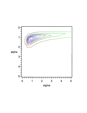
Figure 1: Contour plot of likelihood function (7) on the basis of data in Table 3.

Example 2

Samaniego and Whitaker (1986) presented record data arising from successive failure times of air conditioning units in Boeing aircraft on plan 7914 consists of $n=24$ failure times. The data is given in Table 5.

Table 5: Successive minima, plane 7914.

$i$	1	2	3	4
$R_{i}$	50	44	22	3
$K_{i}$	1	3	2	18

They approximated these data by $Exp(\sigma)$-model and estimated the mean life $\sigma$ as $\hat{\sigma}_{0}=70$. Under $W(\alpha,\sigma)$-model, the MLEs of $\alpha$ and $\sigma$ are obtained as

$$\hat{\alpha}=1.598743046,\ \ \ \hat{\sigma}=51.42746441,$$

respectively. Therefore, $-2\ln\Lambda=1.580279376$ which gives the $p-value=0.2087204561$. This supports exponential assumption by Samaniego and Whitaker (1986). A graph of likelihood function is given in Figure 2.

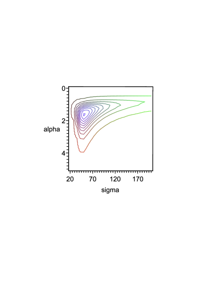
Figure 2: Contour plot of likelihood function (7) on the basis of data in Table 5

Example 3

Samaniego and Whitaker (1988) simulated a random sample with size $n=30$ from $W(\alpha=4,\sigma=1)$-model and record data arising from this sample is presented in Table 6.

Table 6: Simulated record data from $W(\alpha=4,\sigma=1)$.

$i$	1	2	3	4
$R_{i}$	0.879	0.765	0.735	0.220
$K_{i}$	3	2	2	23

Assuming $Exp(\sigma)$-model, MLE of the mean life $\sigma$ is $\hat{\sigma}_{0}=2.67425000$. By assuming $W(\alpha,\sigma)$-model, the MLEs of $\alpha$ and $\sigma$ are obtained as

$$\hat{\alpha}=3.316071956,\ \ \ \hat{\sigma}=0.9728468503,$$

respectively. Therefore, $-2\ln\Lambda=7.911804336$ which gives the $p-value=0.0049113232$. This supports departure from exponential assumption. A graph of likelihood function is given in Figure 3.

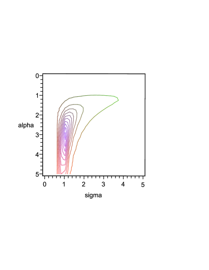
Figure 3: Contour plot of likelihood function (7) on the basis of data in Table 6

6 Concluding Remarks

In this paper, Kolmogorov-Smirnov and Cramer-von Misses type goodness of fit tests as well as a new weighted statistics for record data were proposed. These statistics were used to goodness of fit test for Weibull model. We suggest the following discipline to analyze record data: First step is to test weibull model using the proposed GOF tests in Section 3. Were it accepted, GLR test in Section 4 for the exponentially model. Use the statistical procedures for record data arising from exponential model provided that the exponential model were accepted. See Samaniego and Whitaker (1986), Arnold et. al. (1998), Doostparast (2009), Doostparast and Balakrishnan (2010). If the exponentially was rejected, one can use the results of Hoinkes and Padgett (1994). If the weibull model was rejected, one can use the non-parametric results of Samaniego and Whitaker (1988).

Following Samaniego and Whitaker (1988), one can consider the problem when the available data are arising from $L$ sequence of random variables. More precisely, assume that $L$ independent samples

$$Y_{i1},Y_{i2},\cdots,Y_{i,n_{i}},\ \ \ 1\leq i\leq L,$$

each of size $n_{i}$, are obtained sequentially from $F$. The resulting records are $R_{i1},K_{i1},\cdots$, $R_{im_{i}},K_{im_{i}}$ for $i=1,2,\cdots,L$ where $K_{im_{i}}=n_{i}-\sum_{j=1}^{m_{i}-1}K_{ij}$. Similarly, the NPMLE of the survival function at point $t$ is obtained as

$$\hat{\bar{F}}(t)=\prod_{i:r_{(i)}\leq t}\frac{\sum_{j=i}^{m^{\star}}k_{(j)}-1}{\sum_{j=i}^{m^{\star}}k_{(j)}},$$ (22)

where $m^{\star}=\sum_{i=1}^{L}m_{i}$, $\{r_{(i)},i=1,2,\cdots,m^{\star}\}$ be the order observed record values in the $L$ samples combined and $\{k_{(i)},i=1,2,\cdots,m^{\star}\}$ the induced order statistics for the associated $k_{ij}$. To carry out the impact of $L$ on the power of the GOF tests, one can conduct a simulation study.