Momentum dependence in the dynamically assisted Sauter-Schwinger effect

Abstract

Recently it has been found that the superposition of a strong and slow electric field with a weaker and faster pulse can significantly enhance the probability for non-perturbative electron-positron pair creation out of the vacuum – the dynamically assisted Sauter-Schwinger effect. Via the WKB method, we estimate the momentum dependence of the pair creation probability and compare it to existing numerical results. Besides the theoretical interest, a better understanding of this pair creation mechanism should be helpful for the planned experiments aiming at its detection.

I Introduction

Quantum electrodynamics (QED), the theory of charged particles such as electrons and positrons interacting with the electromagnetic field, offers many interesting phenomena beyond standard perturbation theory (i.e., expansion into powers of the fine-structure constant $\alpha_{\rm QED}$). One prominent example is the Sauter-Schwinger effect Sauter ; Euler ; Schwinger describing the creation of electron-positron pairs out of the QED vacuum by an electric field via tunneling. For a constant electric field $E$, the lowest-order pair creation probability scales as

$$P_{e^{+}e^{-}}\sim\exp\left\{-\pi\,\frac{m^{2}}{qE}\,\frac{c^{3}}{\hbar}\right\}=\exp\left\{-\pi\,\frac{E_{S}}{E}\right\}\,,$$ (1)

where $m$ is the mass and $\pm q$ the charge of the electrons and positrons. Since this expression does not permit a Taylor expansion in $q$, this phenomenon is a non-perturbative effect. Because the characteristic field strength $E_{S}$ (which is also called the critical field) is very large $\sim 10^{18}\rm V/m$, this fundamental QED prediction has not been conclusively experimentally verified yet – in contrast to electron-positron pair creation in the perturbative multi-photon regime, see, e.g., SLAC .

Furthermore, in spite of many efforts, see, e.g., Nikishov+Ritus ; Brezin+Itzykson ; Dumlu ; Keitel ; Hebenstreit ; diverse , our understanding of this non-perturbative effect for non-constant electric fields $E$ is still far from complete. For example, recently it has been found Assisted that the superposition of a strong and slow electric field with a weaker and faster pulse can significantly enhance the pair creation probability, see also Monin+Voloshin ; Catalysis ; Orthaber . In the following, we are going to present an analytic estimate of the momentum dependence of this enhancement mechanism via the WKB approximation (for more details, see also Fey ). These findings should be relevant for the planned experiments with optical lasers or XFEL (or a combination of both), see, e.g., Ringwald , which might facilitate the first conclusive observation of this effect.

II Basic formalism

We consider quantized electrons and positrons in an external (classical) electric field $E$ with no magnetic field present $\mbox{\boldmath$B$}=0$. The field $E$ is supposed to be purely time-dependent $\mbox{\boldmath$E$}=E(t)\mbox{\boldmath$e$}_{x}$ and sub-critical $E\ll E_{S}$. Thus we can neglect the spin of the electrons and positrons and use the Klein-Fock-Gordon equation in temporal gage $\mbox{\boldmath$E$}=\mbox{\boldmath$\dot{A}$}$ where $A$ is the vector potential ($\hbar=c=1$)

$$\left(\frac{\partial^{2}}{\partial t^{2}}-\left[\mbox{\boldmath$\nabla$}-iq\mbox{\boldmath$A$}(t)\right]^{2}+m^{2}\right)\Phi=0\,.$$ (2)

After a spatial Fourier transform, we get momentum

$$\left(\frac{d^{2}}{dt^{2}}+[k_{x}-qA(t)]^{2}+\mbox{\boldmath$k$}_{\perp}^{2}+m^{2}\right)\phi_{\mbox{\boldmath$\scriptstyle k$}}=0\,.$$ (3)

We see that the momentum $\mbox{\boldmath$k$}_{\perp}$ transversal to the electric field can be absorbed by a re-definition of the effective mass $m^{2}\to m_{\rm eff}^{2}=\mbox{\boldmath$k$}_{\perp}^{2}+m^{2}$. Thus, we omit it in the following formulæ for brevity.

The above equation is formally equivalent to a harmonic oscillator with a time-dependent potential

$$\left(\frac{d^{2}}{dt^{2}}+\Omega^{2}(t)\right)\phi(t)=0\,.$$ (4)

If we replace $t$ by $x$, $\phi(t)$ by $\psi(x)$, and $\Omega^{2}(t)$ by $2m[E-V(x)]$, this equation has the same form as a one-dimensional Schrödinger scattering problem with energy $E$ and potential $V(x)$. Therefore, a solution which initially behaves as $\phi_{\mbox{\boldmath$\scriptstyle k$}}^{\rm in}(t)=\exp\{-i\omega_{\mbox{\boldmath$\scriptstyle k$}}t\}$ will finally evolve into a mixture of positive and negative frequencies

$$\phi_{\mbox{\boldmath$\scriptstyle k$}}^{\rm out}(t)=\alpha_{\mbox{\boldmath$\scriptstyle k$}}\exp\{-i\omega_{\mbox{\boldmath$\scriptstyle k$}}t\}+\beta_{\mbox{\boldmath$\scriptstyle k$}}\exp\{+i\omega_{\mbox{\boldmath$\scriptstyle k$}}t\}\,,$$ (5)

where the Bogoliubov coefficients $\alpha_{\mbox{\boldmath$\scriptstyle k$}}$ and $\beta_{\mbox{\boldmath$\scriptstyle k$}}$ are related to the reflection $R$ and transmission $T$ amplitudes in the one-dimensional scattering theory picture via $\alpha_{\mbox{\boldmath$\scriptstyle k$}}=1/T$ and $\beta_{\mbox{\boldmath$\scriptstyle k$}}=R/T$. The probability for electron-positron pair creation is given by $P_{e^{+}e^{-}}=\sum_{\mbox{\boldmath$\scriptstyle k$}}|\beta_{\mbox{\boldmath$\scriptstyle k$}}|^{2}$.

III Riccati equation

For slowly varying and sub-critical electric fields $E(t)$, the Bogoliubov coefficients $\alpha_{\mbox{\boldmath$\scriptstyle k$}}$ and $\beta_{\mbox{\boldmath$\scriptstyle k$}}$ can be derived via the WKB approximation. To this end, let us cast Eq. (4) into a first-order form

$$\frac{d}{dt}\left(\begin{array}[]{c}\phi\\ \dot{\phi}\end{array}\right)=\mbox{\boldmath$\dot{v}$}=\left(\begin{array}[]{cc}0&1\\ -\Omega^{2}(t)&0\end{array}\right)\cdot\left(\begin{array}[]{c}\phi\\ \dot{\phi}\end{array}\right)=\mbox{\boldmath$M$}\cdot\mbox{\boldmath$v$}\,.$$ (12)

Since usual scalar product is not conserved by this evolution equation, it is useful to introduce the inner product

$$(\mbox{\boldmath$v$}|\mbox{\boldmath$v^{\prime}$})=-i(v_{1}^{*}v_{2}^{\prime}-v_{2}^{*}v_{1}^{\prime})\,,$$ (13)

which is just the Wronskian of the original Eq. (4). Thus, the inner product of two solutions $v$ and $v^{\prime}$ is conserved

$$\frac{d}{dt}(\mbox{\boldmath$v$}|\mbox{\boldmath$v^{\prime}$})=0\,.$$ (14)

As the next step, we expand the solution $\mbox{\boldmath$v$}(t)$ of Eq. (12)

$$\mbox{\boldmath$v$}(t)=\alpha(t)e^{i\varphi(t)}\mbox{\boldmath$v$}_{+}(t)+\beta(t)e^{-i\varphi(t)}\mbox{\boldmath$v$}_{-}(t)\,,$$ (15)

into instantaneous eigenvectors $\mbox{\boldmath$v$}_{\pm}(t)$ of the matrix

$$\mbox{\boldmath$M$}\cdot\mbox{\boldmath$v$}_{\pm}(t)=\pm i\Omega(t)\mbox{\boldmath$v$}_{\pm}(t)\,.$$ (16)

With the normalization $\mbox{\boldmath$v$}_{\pm}=(1,\pm i\Omega)^{T}/\sqrt{2\Omega}$, we find $(\mbox{\boldmath$v$}_{+}|\mbox{\boldmath$v$}_{+})=1$, $(\mbox{\boldmath$v$}_{-}|\mbox{\boldmath$v$}_{-})=-1$, and $(\mbox{\boldmath$v$}_{+}|\mbox{\boldmath$v$}_{-})=0$. Finally, $\alpha(t)$ and $\beta(t)$ are the instantaneous Bogoliubov coefficients, where we have separated out the WKB phase

$$\varphi(t)=\int\limits_{-\infty}^{t}dt^{\prime}\,\Omega(t^{\prime})\,.$$ (17)

This uniquely determines the evolution of $\alpha(t)$ and $\beta(t)$ which we can obtain by inserting the expansion (15) into the equation of motion (12) and projecting it with the inner product (13) onto the eigenvectors $\mbox{\boldmath$v$}_{\pm}(t)$

$$\dot{\alpha}(t)=\frac{\dot{\Omega}(t)}{2\Omega(t)}\,e^{-2i\varphi(t)}\beta(t)\,,\;\dot{\beta}(t)=\frac{\dot{\Omega}(t)}{2\Omega(t)}\,e^{2i\varphi(t)}\alpha(t)\,,$$ (18)

where we have used $(\mbox{\boldmath$v$}_{+}|\mbox{\boldmath$\dot{v}$}_{+})=(\mbox{\boldmath$v$}_{-}|\mbox{\boldmath$\dot{v}$}_{-})=0$, as well as $(\mbox{\boldmath$v$}_{-}|\mbox{\boldmath$\dot{v}$}_{+})=\dot{\Omega}/(2\Omega)$ and $(\mbox{\boldmath$v$}_{+}|\mbox{\boldmath$\dot{v}$}_{-})=-\dot{\Omega}/(2\Omega)$. In terms of the reflection coefficient $R(t)=\beta(t)/\alpha(t)$, we get

$$\dot{R}(t)=\frac{\dot{\Omega}(t)}{2\Omega(t)}\left(e^{2i\varphi(t)}-R^{2}(t)e^{-2i\varphi(t)}\right)\,,$$ (19)

which is known as Riccati equation, see also Dumlu ; Riccati .

IV WKB method

The Riccati equation (19) is still exact but unfortunately non-linear. The WKB approximation is based on the assumption that the rate of change of $\Omega(t)$ is much slower than the internal frequency $\Omega(t)$ itself. In our case,

$$\Omega^{2}(t)=[k_{x}-qA(t)]^{2}+m^{2}\,,$$ (20)

this is satisfied if the strength $E$ and the rate of change $\omega$ of the electric field $E(t)$ are small compared to the mass, i.e., for $E\ll E_{S}$ and $\omega\ll m$. In this limit, the phase factors $e^{\pm 2i\varphi}$ are rapidly oscillating and the magnitude of $R$ can be estimated by analytic continuation to the complex plane. In terms of the phase variable $\varphi$, the Riccati equation (19) reads

$$\frac{dR(\varphi)}{d\varphi}=\frac{1}{2}\left(e^{2i\varphi}-R^{2}(\varphi)e^{-2i\varphi}\right)\frac{d\ln\Omega(\varphi)}{d\varphi}\,.$$ (21)

Now analytic continuation to the upper complex half-plane $\varphi\to\Re\varphi+i\Im\varphi=\Re\varphi+i\chi$ shows that $R$ becomes exponentially suppressed $R\sim e^{-2\chi}$. The degree of this suppression depends on the point where the analytic continuation breaks down. Since $e^{\pm 2i\varphi}$ is analytic everywhere, this will be determined by the term $\ln\Omega$. Typically, one can go into the upper complex half-plane until one hits the first zero of $\Omega$ at $t_{*}$, i.e., $\Omega(t_{*})=0$. These points $t_{*}$ in the complex plane are analogous to the classical turning points in WKB. Consequently, we find

$$R(t\uparrow\infty)=R\sim e^{-2\chi_{*}}=\exp\left\{-2\Im\left[\varphi(t_{*})\right]\right\}\,.$$ (22)

So far, this is only an order-of-magnitude estimate. However, it can be shown Davis that this expression becomes exact (under appropriate conditions) in the adiabatic limit (roughly speaking, $m\uparrow\infty$), i.e., that the pre-factor in front of the exponential tends to one.

In case of more than one turning point, the one with the smallest $\chi_{*}$, i.e., closest to real axis (in the complex $\varphi$-plane) dominates. For multiple turning points with similar $\chi_{*}$, there can be interference effects Dumlu ; Hebenstreit .

V Double Sauter pulse

Now we are in the position to apply the above method to the double Sauter pulse studied in Assisted

$$E(t)=\frac{E_{1}}{\cosh^{2}(\omega_{1}t)}+\frac{E_{2}}{\cosh^{2}(\omega_{2}t)}\,.$$ (23)

Note that the Dirac equation in the presence of a single pulse (e.g., $E_{2}=0$) of that type can be solved exactly. This solution has already been used by Sauter Sauter even though with $t$ and $x$ interchanged.

The first term on the r.h.s. describes a strong and slow electric field profile while the second term corresponds to a much weaker and faster pulse with $\omega_{1}\ll\omega_{2}\ll m$ and $E_{2}\ll E_{1}\ll E_{S}$. The Keldysh Keldysh parameters of the two pulses are supposed to be small $\gamma_{1}=m\omega_{1}/(qE_{1})\ll 1$ and large $\gamma_{2}=m\omega_{2}/(qE_{2})\gg 1$, respectively, while the combined Keldysh parameter introduced in Assisted

$$\gamma_{\rm c}=\frac{m\omega_{2}}{qE_{1}}\,,$$ (24)

is of order one. For time scales where the second (fast) pulse contributes, we may approximate the first (slow) pulse by a constant field $E_{1}$ due to $\omega_{1}\ll\omega_{2}$. Thus the vector potential becomes

$$A(t)\approx E_{1}t+\frac{E_{2}}{\omega_{2}}\,\tanh(\omega_{2}t)\,,$$ (25)

and the condition $\Omega(t_{*})=0$ for the turning points reads

$$\omega_{2}t_{*}+\frac{E_{2}}{E_{1}}\,\tanh(\omega_{2}t_{*})=\gamma_{\rm c}\left(i+\frac{k_{x}}{m}\right)\,.$$ (26)

Due to the periodicity of the function $\tanh(\omega_{2}t)$, there are infinitely many solutions. However, we are mainly interested in those close to the real axis – which have the smallest value of $\chi_{*}$. For $E_{1}\gg E_{2}$, we may approximate the two most relevant solutions $t_{*}$ and $t_{*}^{\prime}$ via

$$t_{*}\approx\frac{m}{qE_{1}}\left(i+\frac{k_{x}}{m}\right)\,,\quad t_{*}^{\prime}\approx\frac{i\pi}{2\omega_{2}}\,.$$ (27)

Note that this approximation breaks down when $\gamma_{\rm c}$ approaches $\pi/2$, so we will assume $\gamma_{\rm c}>\pi/2$ in the following, see also Assisted . The first solution $t_{*}$ is basically the same as for the slow pulse alone (i.e., $E_{2}=0$), while the second one $t_{*}^{\prime}$ is obviously tied to the fast pulse.

Again using $E_{1}\gg E_{2}$, we may derive the associated exponents $\chi_{*}$ and $\chi_{*}^{\prime}$. For the normal solution $t_{*}$, we reproduce the usual value given solely by the slow pulse

$$\chi_{*}=\frac{\pi m^{2}}{4qE_{1}}\,.$$ (28)

With $P_{e^{+}e^{-}}\sim|\beta_{\mbox{\boldmath$\scriptstyle k$}}^{2}|\approx|R^{2}|\sim e^{-4\chi_{*}}$, we verify Eq. (1). This result is independent of $k_{x}$ because we have approximated the slow pulse by a constant field. The anomalous solution $t_{*}^{\prime}$, on the other hand, yields

$$\chi_{*}^{\prime}=\frac{m^{2}}{2qE_{1}}\,\Im\left\{f\left(\frac{i\pi}{2\gamma_{\rm c}}-\frac{k_{x}}{m}\right)\right\}\,,$$ (29)

with $f(x)=x\sqrt{1+x^{2}}+{\rm arcsinh}(x)$. In this form, the dependence on $k_{x}$ is perhaps not so obvious. Thus, let us Taylor expand this expression in powers of $k_{x}$

$$\chi_{*}^{\prime} = \frac{m^{2}}{2qE_{1}}\left[\frac{\pi}{2\gamma_{\rm c}}\sqrt{1-\left(\frac{\pi}{2\gamma_{\rm c}}\right)^{2}}+{\rm arcsin}\left(\frac{\pi}{2\gamma_{\rm c}}\right)\right]+$$ (30)

$$+\frac{k_{x}^{2}}{2qE_{1}}\,\frac{\pi}{\sqrt{4\gamma_{\rm c}^{2}-\pi^{2}}}+\,{\cal O}(k_{x}^{4})\,.$$

The momentum-independent result in the first line was already derived in Assisted via the word-line instanton method, but this method did not yield any information about the momentum dependence in the second line.

VI Discussion

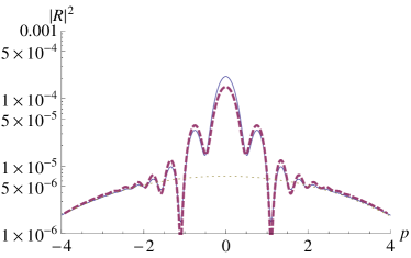
Figure 1: (Color online) Comparison of analytical and numerical results for the (differential) pair creation probability $|R|^{2}$ depending on the momentum $p=k_{x}/m_{\rm eff}$. The solid (blue) curve shows the numerical data from Orthaber (kindly provided by the authors) for $E_{1}=E_{S}/4$, $\omega_{1}=10^{4}\rm eV$, $E_{2}=E_{1}/10$, and $\omega_{2}=5\times 10^{5}\rm eV$. For the same values, the function $|R|^{2}=|c_{*}\exp\{-2\varphi(t_{*})\}+c_{*}^{\prime}\exp\{-2\varphi(t_{*}^{\prime})\}|^{2}$ representing the WKB result is plotted (dashed purple curve), where $t_{*}$ and $t_{*}^{\prime}$ are the (exact) WKB turning points and $\varphi$ is the complex phase in Eq. (17). The pre-factors are chosen as $c_{*}=1.4$ and $c_{*}^{\prime}=0.2$. Finally, the dotted (brown) curve describes the case $E_{2}=0$ of a single pulse (i.e., the background).

For the dynamically assisted Sauter-Schwinger effect Assisted , we estimated the momentum dependence in Eqs. (29) and (30) via the WKB method. The strong and slow pulse alone is represented by the normal turning point $t_{*}$ with $\chi_{*}$ in Eq. (28). It has a broad momentum distribution $(\Delta k_{x})^{2}/m^{2}\sim 1/\gamma_{1}^{2}\gg 1$ which can be explained by the uncertainty $\Delta t\sim 1/\omega_{1}$ of the creation time: Particles that are created earlier have more time to be accelerated by the strong electric field than others which are produced later momentum . The dynamically assisted effect, on the other hand, corresponds to the anomalous turning point $t_{*}^{\prime}$ determined by the weak and fast pulse. Thus, the creation time is far less uncertain $\Delta t\sim 1/\omega_{2}$ and – as one would expect – it has a much narrower width, even though it is probably hard to guess the precise scaling $(\Delta k_{x})^{2}\sim qE\sqrt{4\gamma_{\rm c}^{2}-\pi^{2}}$ beforehand. Consistent with Assisted , this window closes for $\gamma_{\rm c}\downarrow\pi/2$, after which the enhancement disappears. For $\gamma_{\rm c}<\pi/2$, the normal turning point $t_{*}$ dominates $\chi_{*}<\chi_{*}^{\prime}$.

Let us compare our findings with the numerical results in Orthaber obtained via the quantum kinetic approach. In Fig. 1, we plot the numerical data from Fig. 5a of Orthaber as well as $|R|^{2}=|c_{*}\exp\{-2\varphi(t_{*})\}+c_{*}^{\prime}\exp\{-2\varphi(t_{*}^{\prime})\}|^{2}$, where $\varphi$ is the complex phase in Eq. (17). The two WKB turning points $t_{*}$ and $t_{*}^{\prime}$ can be obtained exactly, but our WKB method does not yield the pre-factors $c_{*}$ and $c_{*}^{\prime}$, which can also depend on $p$ in general. Neglecting this $p$-dependence, we may estimate the normal pre-factor $c_{*}$ by comparison to the case of a single pulse (i.e., $E_{2}=0$) which facilitates an analytic solution. The anomalous pre-factor $c_{*}^{\prime}$, on the other hand, was chosen (fitted) to match the numerical results. After that, the agreement between the analytic and the numerical results is surprisingly good – given that the employed values $E_{1}=E_{S}/4$, $\omega_{1}=10^{4}\rm eV$, $E_{2}=E_{1}/10$, and $\omega_{2}=5\times 10^{5}\rm eV$ do not satisfy our underlying assumptions $E_{2}\ll E_{1}\ll E_{S}$ and $\omega_{1}\ll\omega_{2}\ll m$ very well. Note that the difference between $c_{*}$ and $c_{*}^{\prime}$ also indicates that we are not deep in the adiabatic limit ($m\uparrow\infty$). Furthermore, one should be very careful with the order of the various limits in this multiple-scale problem. For example, the adiabatic limit ($m\uparrow\infty$) does not commute with the limit $E_{2}/E_{1}\downarrow 0$ since the dynamically assisted Sauter-Schwinger effect given by $c_{*}^{\prime}$ should vanish for $E_{2}=0$. Finally, the oscillations visible in Fig. 1 (and Fig. 5a of Orthaber ) can be explained nicely by interference effects Dumlu ; Hebenstreit of the two turning points $t_{*}$ and $t_{*}^{\prime}$. The interferences are most pronounced where the two contributions $c_{*}\exp\{-2\varphi(t_{*})\}$ and $c_{*}^{\prime}\exp\{-2\varphi(t_{*}^{\prime})\}$ are equally strong, which happens around $k_{x}\approx\pm m_{\rm eff}$ in this case.

VII Outlook

It might be interesting to generalize the above findings to other pulse profiles such as

$$E(t)=E_{1}f_{1}(\omega_{1}t)+E_{2}f_{2}(\omega_{2}t)\,,$$ (31)

with $f_{1}(0)=f_{2}(0)=1$ as well as $\omega_{1}\ll\omega_{2}\ll m$ and $E_{2}\ll E_{1}\ll E_{S}$. For a broad class of functions, for example $f_{2}(x)=1/(1+x^{2})^{2}$, we expect to obtain qualitatively the same picture as discussed above. Again, the normal turning point $t_{*}$ will have basically the same value as in Eq. (27) and the anomalous turning point $t_{*}^{\prime}$ will be very close to the singularity of $f_{2}$, in our example $t_{*}^{\prime}\approx i/\omega_{2}$. As before, for small values of the combined Keldysh parameter $\gamma_{\rm c}$ in Eq. (24), the contribution of the normal turning point $t_{*}$ dominates – but if $\gamma_{\rm c}$ exceeds a critical value of order one, the anomalous turning point $t_{*}^{\prime}$ becomes stronger than the normal one and we get dynamically assisted pair creation.

For other profiles, such as $f_{2}(x)=\exp\{-x^{2}\}$, however, the anomalous turning point $t_{*}^{\prime}$ logarithmically depends on the ratio $E_{1}/E_{2}$ and thus the mechanism of dynamically assisted pair creation (including the threshold value for $\gamma_{\rm c}$) will also depend on $E_{1}/E_{2}$, in contrast to the case considered above.

- (1) F. Sauter, Z. Phys. 69, 742 (1931); ibid. 73, 547 (1931).
- (2) W. Heisenberg and H. Euler, Z. Phys. 98, 714 (1936).
- (3) J. Schwinger, Phys. Rev. 82, 664 (1951).
- (4) D.L. Burke et al, Phys. Rev. Lett. 79, 1626 (1997).
- (5) A. I. Nikishov and V. I. Ritus, Sov. Phys. JETP 25, 1135 (1967).
- (6) E. Brezin and C. Itzykson, Phys. Rev. D 2, 1191 (1970);
- (7) C.K. Dumlu and G.V. Dunne, Phys. Rev. D 83, 065028 (2011); Phys. Rev. Lett. 104, 250402 (2010); C.K. Dumlu, Phys. Rev. D 82, 045007 (2010); E. Akkermans, G. V. Dunne, arXiv:1109.3489.
- (8) M. Ruf et al, Phys. Rev. Lett. 102, 080402 (2009).
- (9) F. Hebenstreit, R. Alkofer, G.V. Dunne, and H. Gies, Phys. Rev. Lett. 102, 150404 (2009).
- (10) F. V. Bunkin and I. I. Tugov, Sov. Phys. Dokl. 14, 678 (1970); N. B. Narozhnyi and A. I. Nikishov, Sov. J. Nucl. Phys. 11, 596 (1970); V. S. Popov, JETP Lett. 13, 185 (1971); ibid. 18, 255 (1973); W. Becker et al., Adv. Atom. Mol. Opt. Phys. 48, 35 (2002). S. P. Kim and D. N. Page, Phys. Rev. D 65, 105002 (2002); ibid. 75, 045013 (2007); N. B. Narozhny, S. S. Bulanov, V. D. Mur, and V. S. Popov, Phys. Lett. A 330, 1 (2004); JETP Lett. 80, 382 (2004); H. Gies and K. Klingmuller, Phys. Rev. D 72, 065001 (2005). G. V. Dunne and C. Schubert, ibid. 72, 105004 (2005); G. V. Dunne, Eur. Phys. J. D, 55, 327 (2009); L. Labun and J. Rafelski, Phys. Rev. D 84, 033003 (2011); F. Hebenstreit, R. Alkofer and H. Gies, Phys. Rev. Lett. 107, 180403 (2011).
- (11) R. Schützhold, H. Gies, and G. Dunne, Phys. Rev. Lett. 101, 130404 (2008).
- (12) A. Monin and M.B. Voloshin, Phys. Rev. D 81, 025001 (2010).
- (13) G. V. Dunne, H. Gies, R. Schützhold, Phys. Rev. D 80, 111301 (2009).
- (14) M. Orthaber, F. Hebenstreit, R. Alkofer, Phys. Lett. B 698, 80 (2011).
- (15) C. Fey, Dynamisch verstärkter Schwinger-Effekt, BSc-Thesis, Universität Duisburg-Essen (2011).
- (16) For XFELs, see, e.g., A. Ringwald, Phys. Lett. B 510, 107 (2001); and for optical lasers, see, e.g., http://www.extreme-light-infrastructure.eu
- (17) Since Eq. (2) is spatially homogeneous, the canonical momentum is conserved – but the physical momentum is not (as the particles are accelerated by the electric field).
- (18) Strictly speaking, Eq. (19) is the Riccati equation for scalar QED since we started from the Klein-Fock-Gordon equation (2) and thus neglected the spin of the electrons and positrons. Taking their spin into account, the Riccati equation for spinor QED has the same form as Eq. (19) after replacing by another time-dependent function, see, e.g., Dumlu . However, since the exponential dependence and the location of the singularities is the same in both cases, the WKB exponents calculated here remain unchanged, only the pre-factors (including relative phases) may be different.
- (19) J. P. Davis and P. Pechukas, J. Chem. Phys. 64, 3129 (1976); see also S. Massar and R. Parentani, Nucl. Phys. B 513, 375 (1998) and references therein.
- (20) L. V. Keldysh, Sov. Phys. JETP 20, 1307 (1965).