A far-infrared survey of bow shocks and detached shells around AGB stars and red supergiants 

Abstract

Aims. Our goal is to study the different morphologies associated to the interaction of stellar winds of AGB stars and red supergiants with the interstellar medium (ISM) to follow the fate of the circumstellar matter injected into the interstellar medium.

Methods. Far-infrared Herschel/PACS images at 70 and 160 $\mu$m of a sample of 78 Galactic evolved stars are used to study the (dust) emission structures, originating from stellar wind-ISM interaction. In addition, two-fluid hydrodynamical simulations of the coupled gas and dust in wind-ISM interactions are used to compare with the observations.

Results. Four distinct classes of wind-ISM interaction (i.e. “fermata”, “eyes”, “irregular”, and “rings”) are identified and basic parameters affecting the morphology are discussed. We detect bow shocks for $\sim$40% of the sample and detached rings for $\sim$20%. The total dust and gas mass inferred from the observed infrared emission is similar to the stellar mass loss over a period of a few thousand years, while in most cases it is less than the total ISM mass potentialy swept-up by the wind-ISM interaction. De-projected stand-off distances ($R_{0}$) – defined as the distance between the central star and the nearest point of the interaction region – of the detected bow shocks (“fermata” and “eyes”) are derived from the PACS images and compared to previous results, model predictions and the simulations. All observed bow shocks have stand-off distances smaller than 1 pc. Observed and theoretical stand-off distances are used together to independently derive the local ISM density.

Conclusions. Both theoretical (analytical) models and hydrodynamical simulations give stand-off distances for adopted stellar properties that are in good agreement with the measured de-projected stand-off distance of wind-ISM bow shocks. The possible detection of a bow shock – for the distance limited sample – appears to be governed by its physical size as set roughly by the stand-off distance. In particular the star’s peculiar space velocity and the density of the ISM appear decisive in detecting emission from bow shocks or detached rings. In most cases the derived ISM densities concur with those typical of the warm neutral and ionised gas in the Galaxy, though some cases point towards the presence of cold diffuse clouds. Tentatively, the “eyes” class objects are associated to (visual) binaries, while the “rings” generally appear not to occur for M-type stars, only for C or S-type objects that have experienced a thermal pulse.

1 Introduction

The chemical enrichment of the Universe plays an important role in explaining stellar and galaxy evolution. Apart from supernovae, asymptotic giant branch (AGB) stars and supergiants play a crucial role in supplying heavy elements into the interstellar medium (ISM). It has been well established that evolved stars lose material during their AGB and supergiant phase via a dusty wind, and this wind material will eventually be dissipated into the ISM (e.g. Tielens et al. 2005). The presence of extended envelopes around AGB stars and supergiants is a direct result of their stellar mass loss. The properties of these (detached) shells are directly affected by the mass-loss history of low- to intermediate-mass stars and thus contain information on this late stage of stellar evolution.

Both the chemical composition and physical conditions of the stellar-wind material returned to the ISM can be altered by several processes, such as mixing of nucleosynthesis products into the envelope, dust formation (Ferrarotti & Gail 2006), shock-induced chemistry in the inner wind envelope (Duari et al. 1999), as well as photo-dissociation due to interstellar cosmic rays and UV photons penetrating the outer envelope (Willacy & Millar 1997; Decin et al. 2010). There is a marked difference between the dust and gas formed in circumstellar environments and that present in the ISM (e.g. Jones 2001). To reconcile these differences in the composition of circumstellar and interstellar dust additional processes are expected to play an important role. One such mechanism involves processing and alteration of dust in shocks that can occur when the stellar wind material interacts with the local ISM. Shocks are not only important in that they can alter the composition of the dusty wind but they also generate turbulence and acoustic noise, which affect the evolution of the ISM (Cox & Smith 1974; McKee & Ostriker 1977) and are believed to be of importance to the initial phases of star formation (McKee & Cowie 1975; Spitzer 1982).

IRAS observations already hinted at the existence of low temperature circumstellar dust (van der Veen & Habing 1988). Clear observational evidence for detached shells around evolved stars was found by e.g. Olofsson et al. (1988); Stencel et al. (1988); Hawkins (1990). Following these discoveries, infrared observations with IRAS and ISO revealed a growing number of AGB stars with extended and sometimes clearly detached thermal dust emission (e.g. Young et al. 1993b, a; Waters et al. 1994; Izumiura et al. 1996; Hashimoto & Izumiura 1998). At the same time, CO radio line emission revealed a number of objects with detached gas shells (Olofsson 1996, and references therein). A number of detached-shell objects was also imaged in the optical (e.g. González Delgado et al. 2001; Maercker et al. 2010; Olofsson et al. 2010). Interferometric radio maps uncovered their detailed structure, which turned out to be remarkable spherical thick CO-line-emitting, geometrically-thin shells (Lindqvist et al. 1999; Olofsson et al. 2000). These observations showed that possibly short phases of intense mass-loss rate are required to form such large detached (spherical) molecular shells of swept up wind and interstellar material (Rowan-Robinson et al. 1986; Zijlstra & Weinberger 2002; Libert et al. 2007). The enhanced mass-loss rate events could be induced by a thermal pulse (van der Veen & Habing 1988; Vassiliadis & Wood 1993) or, alternatively, the He core-flash at the end of the RGB phase (Dominy 1984).

IRAS also observed for the first time the infrared signatures of bow shocks associated to e.g. ultra-compact H ii regions (van Buren et al. 1990; Mac Low et al. 1991) and runaway OB stars (Noriega-Crespo et al. 1997). Stencel et al. (1988) presented the first IRAS detection of a bow shock around a red supergiant, $\alpha$ Ori. These data were re-processed by Noriega-Crespo et al. (1997) which revealed a detached bow shock at $\sim$6′ as well as a linear bar at 9′. Only recently, infrared space telescopes such as Spitzer and AKARI reveal much more detail on the infrared signatures of bow shocks around evolved stars, such as R Hya (Ueta et al. 2006), $\alpha$ Ori (Ueta et al. 2008), R Cas (Hashimoto & Izumiura 1998; Ueta et al. 2010), and U Hya (Izumiura et al. 2011). The Herschel Space Observatory now reveals these infrared shells and bow shock regions at the best spatial resolution ever. Detached infrared shells around TT Cyg, U Ant, and AQ And are discussed in Kerschbaum et al. (2010) and on more objects in Kerschbaum et al. (2011). Bow shocks are reported for CW Leo (Ladjal et al. 2010), X Her and TX Psc (Jorissen et al. 2011), and $\alpha$ Ori (Decin et al. in preparation). For $o$ Cet the inner part of the stellar wind bubble bounded and formed by the termination shock is seen (Mayer et al. 2011). For some of these infrared bow shocks, counterparts are detected in UV emission ($o$ Cet: Martin et al. 2007; CW Leo: Sahai & Chronopoulos 2010). These observations indicate that the wind material undergoes additional processing in wind-ISM shocks and that such processing is perhaps more common than previously envisioned.

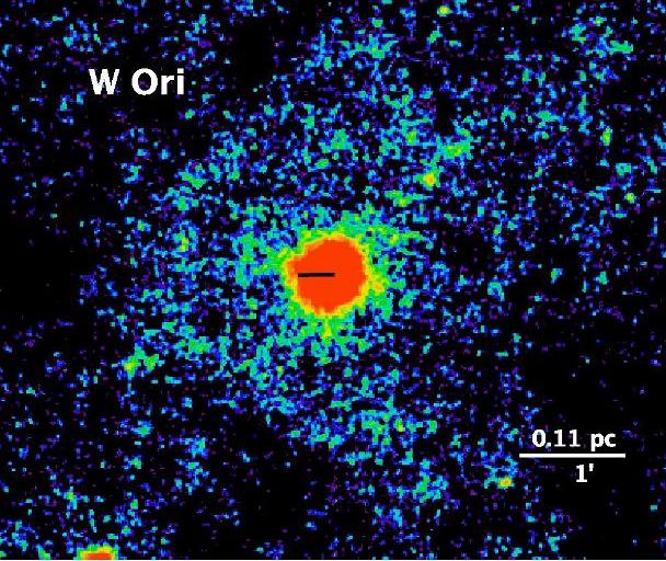
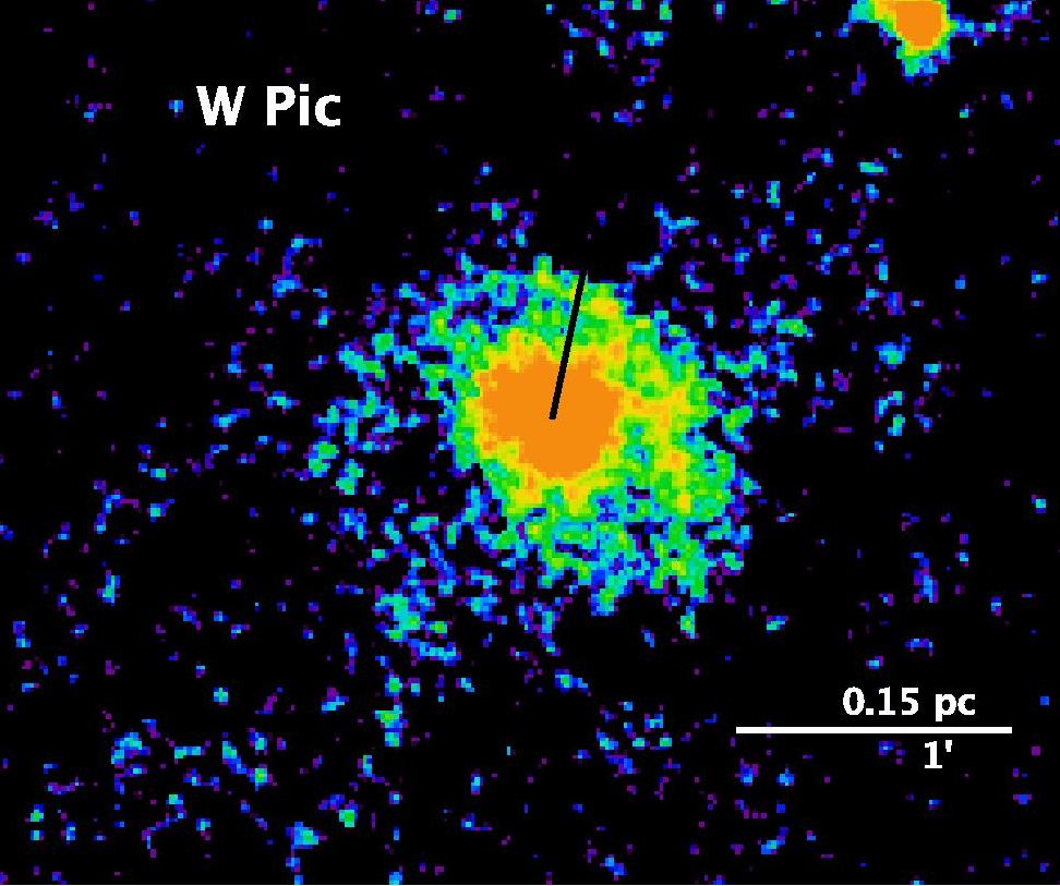
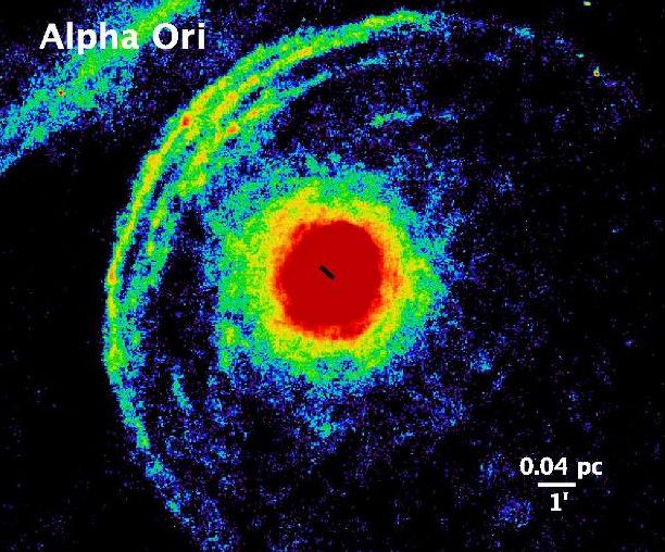
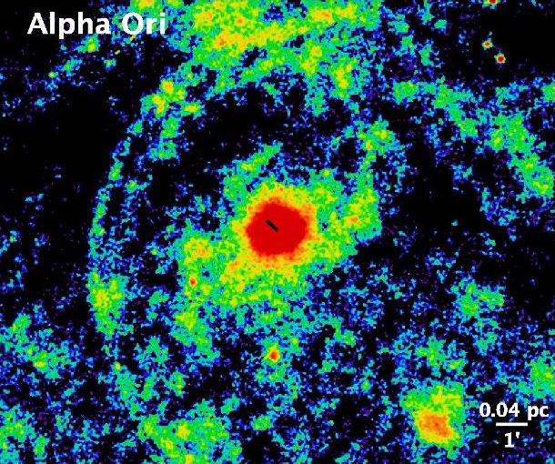
Figure 1: Interaction type “fermata” (Class I). PACS 70 $\mu$m (left) and 160 $\mu$m (right). The white horizontal bar in each panel is 1′ in length, annotated with the corresponding physical size. All panels have north up and east to the left. The black line indicates the direction of the space velocity of the star (adopting a scale such that 1 km s^-1 corresponds to 1″on the image). Note: R Scl also has an inner spherical shell (not visible here). One needs to multiply flux values by $4.25\cdot 10^{4}$ to convert from Jy arcsec^-2 to MJy sr^-2.

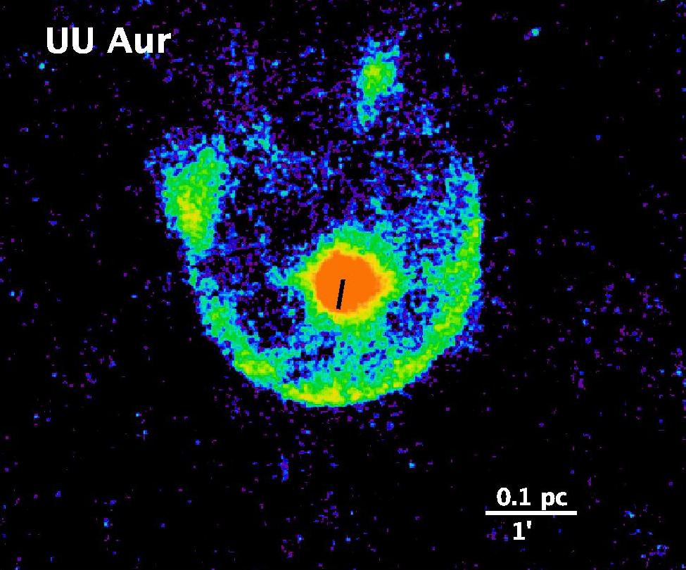
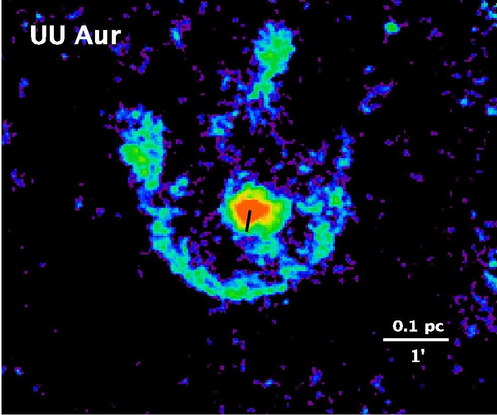
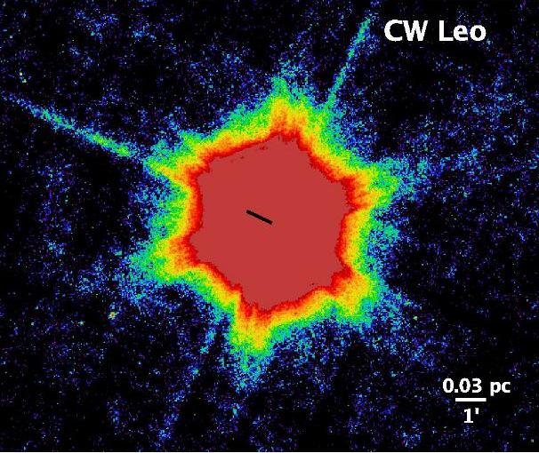
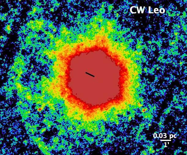
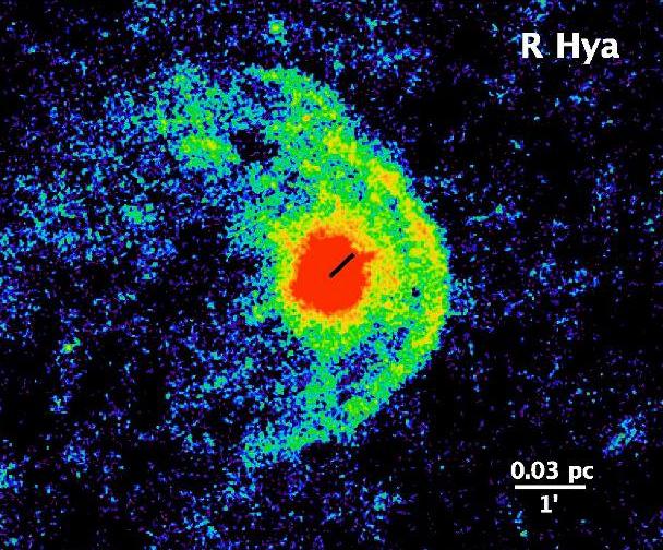
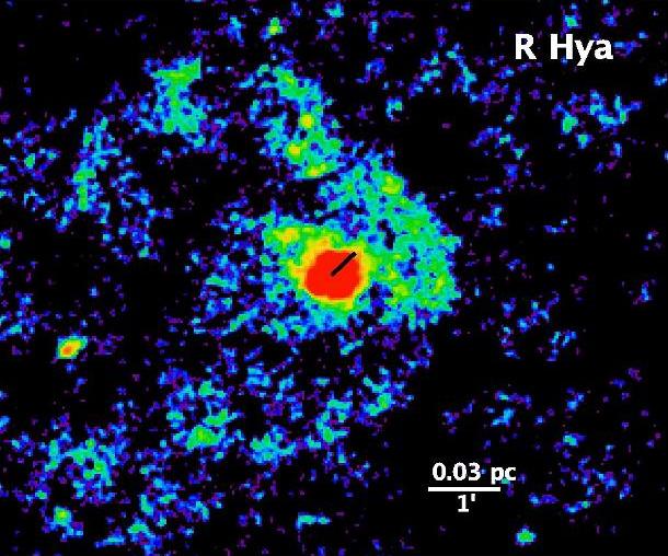
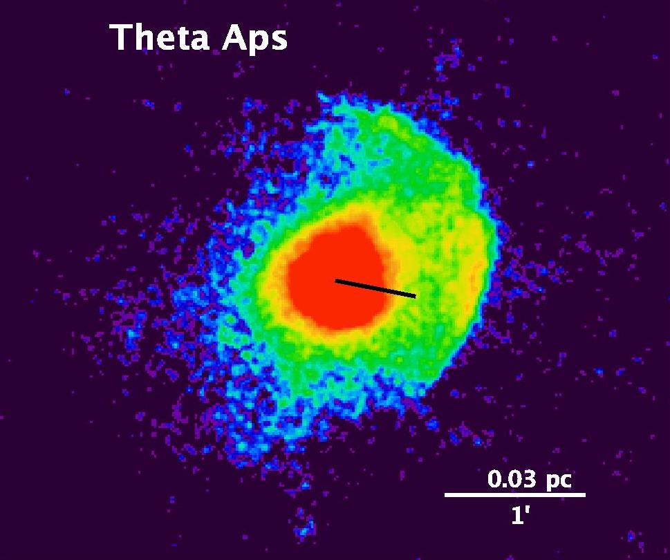
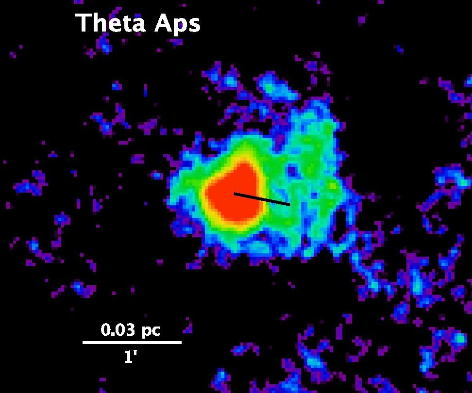
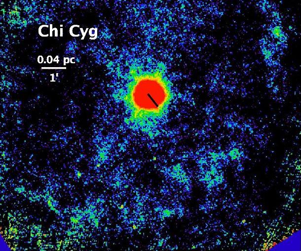
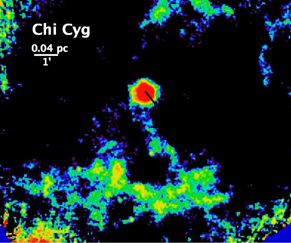
Figure 1: (continued). Interaction type “fermata” (Class I). PACS 70 $\mu$m (left) and 160 $\mu$m (right). For CW Leo see also Ladjal et al. (2010) and for $\alpha$ Ori see Decin et al. (in preparation). The bow shock of $\chi$ Cyg is at several arcminutes to the south (not readily discernible in the image).

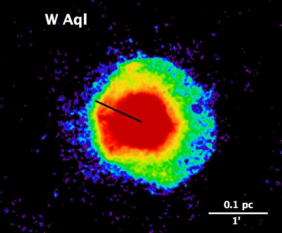
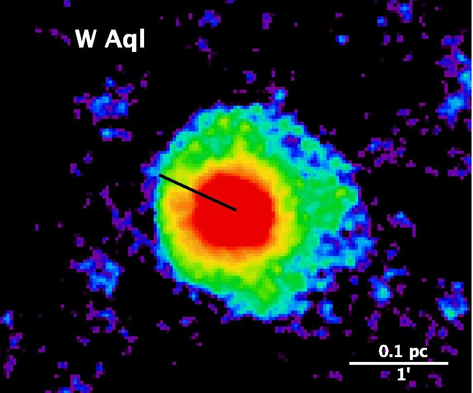
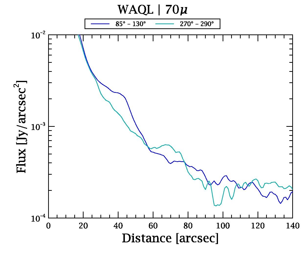
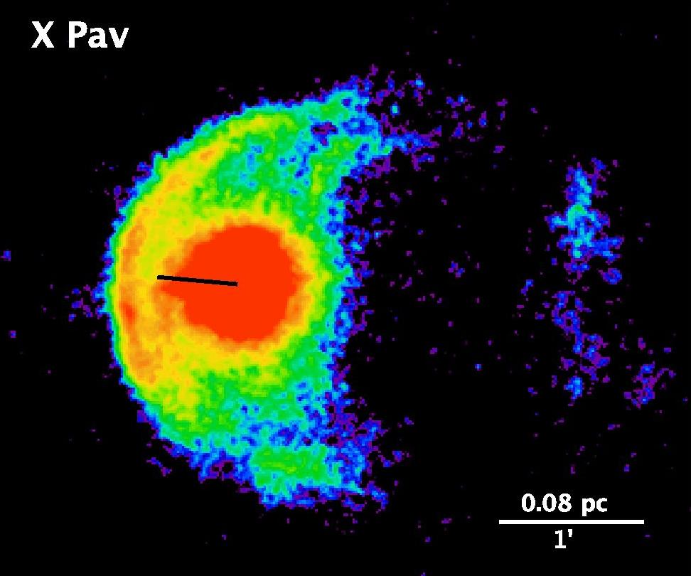
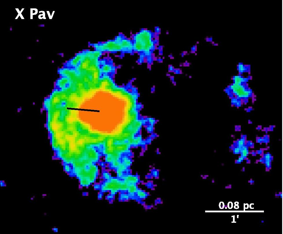
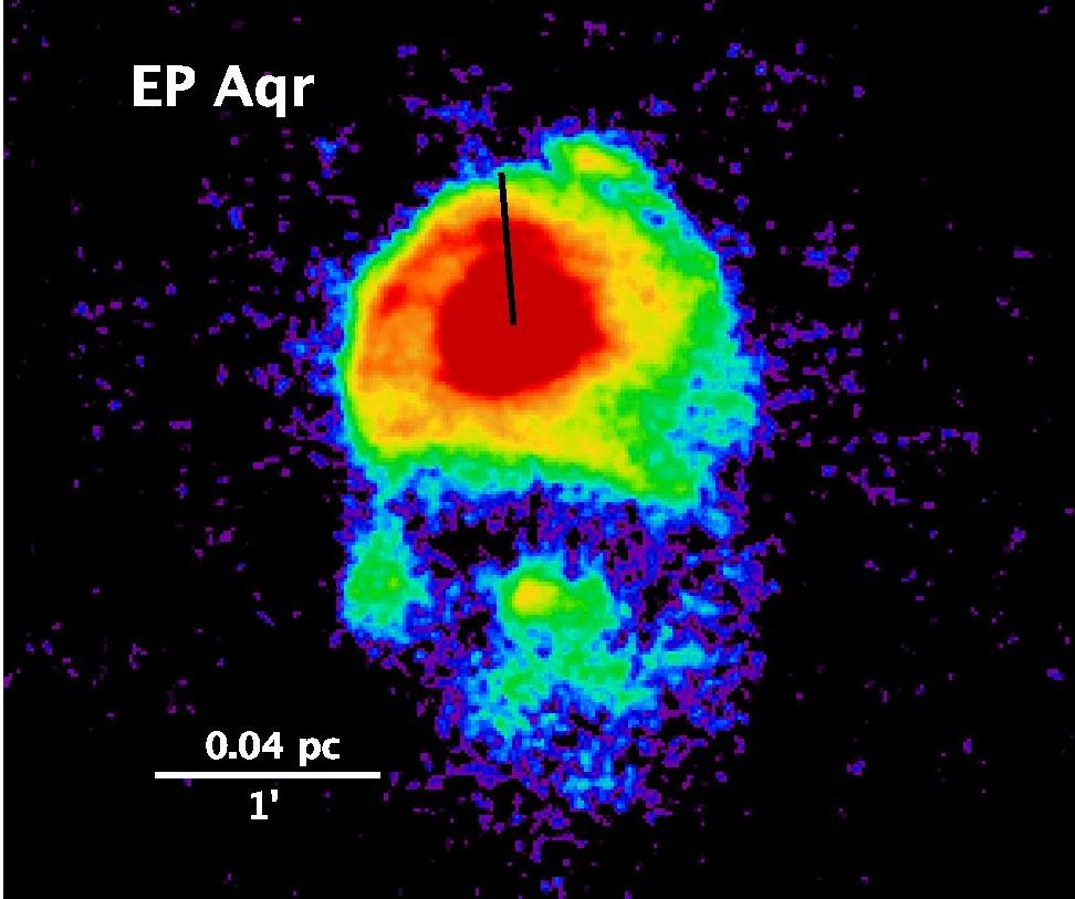
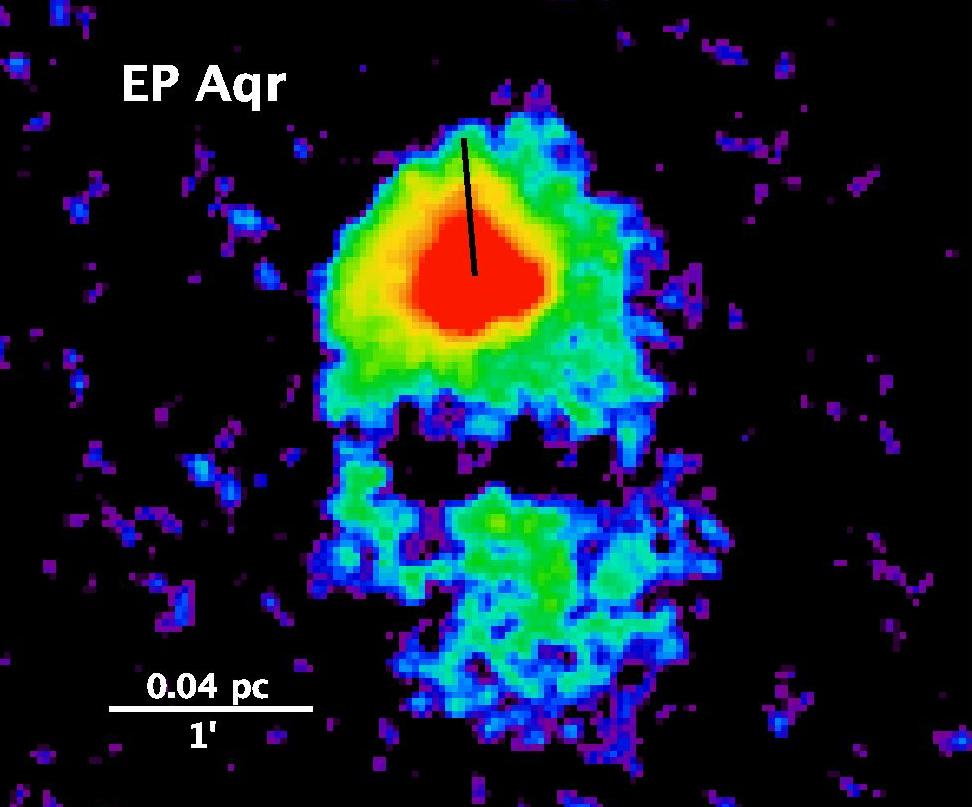
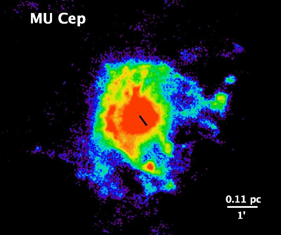
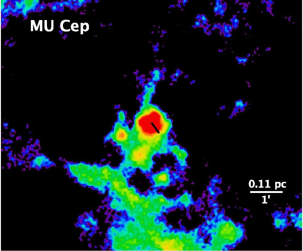
Figure 1: (continued). Interaction type “fermata” (Class I). PACS 70 $\mu$m (left) and 160 $\mu$m (right). Radial profiles (azimuthally averaged over two opening angle ranges: 85-130° and 270-290°) are shown for 70 $\mu$m image of W Aql (bottom right). Note the presence of turbulent instabilities in $\mu$ Cep.

This paper presents the properties – such as morphology, size, and brightness – of detached or spatially extended far-infrared emission associated to bow shock interaction regions and detached shells around a large sample of AGB stars and red supergiants. The paper is structured as follows. First we discuss the observations, the data processing and map-reconstruction scheme, and present the infrared images in Sect. 2. In Sect. 3.1 we introduce a simple morphological classification system differentiating observed shapes, in particular we make a distinction between bow shocks and detached rings. In Sects. 3.2 and 3.3 we present radial profiles as well as infrared flux measurements of the extended emission. In order to make a qualitative and quantitative comparison of the observed bow shocks and detached rings we review first the basic physics and relevant stellar and interstellar parameters underlying the formation of a bow shock or detached shell (Sect. 4). In Sect. 5 we discuss and collect the relevant parameters in order to predict, for example, the size of the bow shock. Next, in Sect. 6, we present hydrodynamical simulations to elaborate on the origin of the observed morphologies, in particular, the features related to (turbulent) instabilities. The observations are compared to the theoretical predictions and the simulations in Sect. 7. Furthermore, the observations are interpreted in the context of stellar mass-loss and ISM properties as well as with respect to the interaction between these two material flows. Then we discuss the requirements to observe wind-ISM interaction, and thus address the frequent occurrence of bow shocks for our entire sample of AGB stars and red supergiants. The main results and conclusions are summarised in Sect. 8.

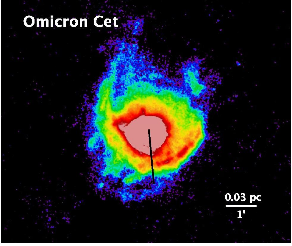
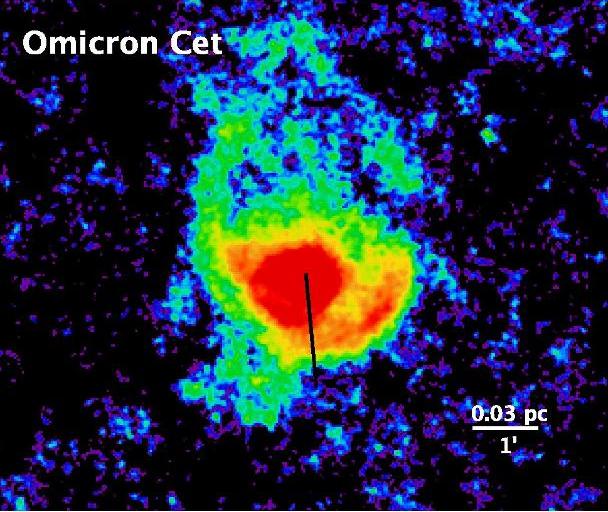
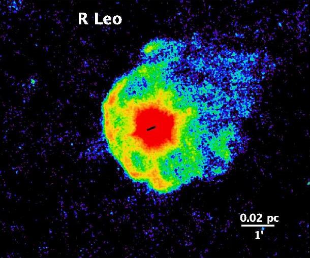
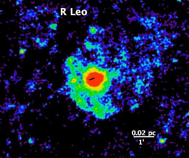
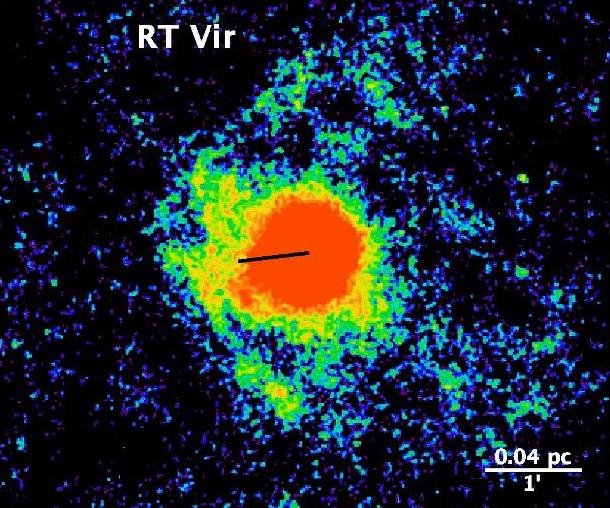
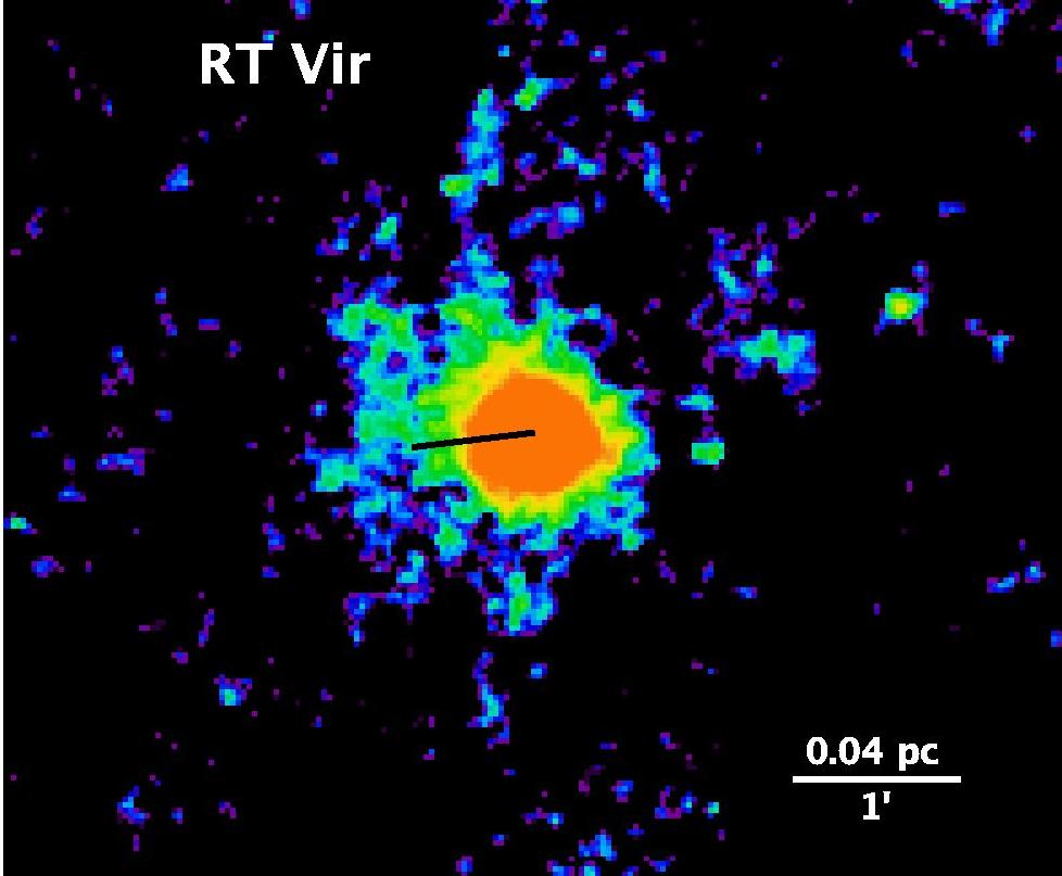
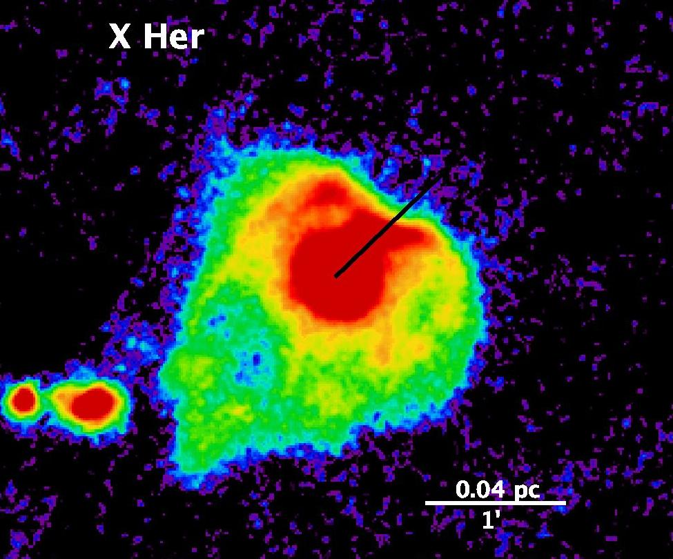
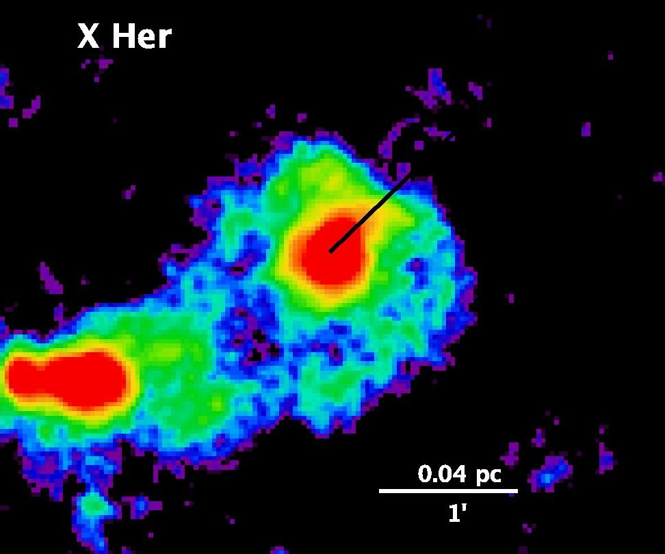
Figure 1: (continued). Interaction type “fermata” (Class I). PACS 70 $\mu$m (left) and 160 $\mu$m (right). $o$ Cet, R Leo, RT Vir, and X Her reveal RT and/or KH instabilities. For $o$ Cet see also Mayer et al. (2011). The sources visible eastward of X Her are background galaxies (see also Jorissen et al. 2011).

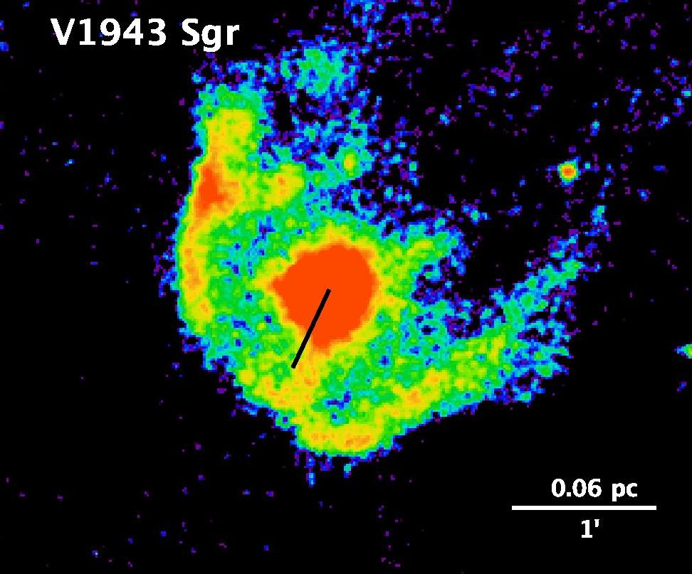
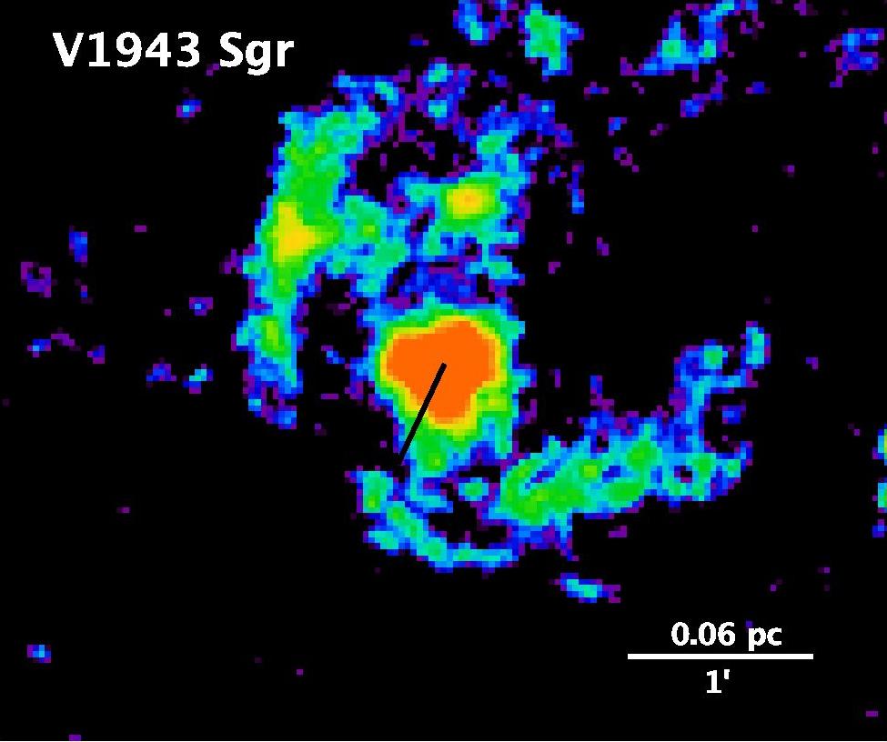
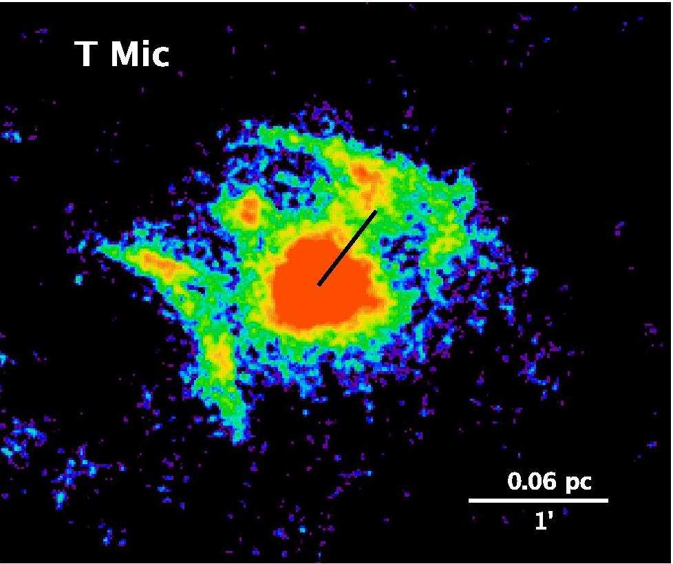
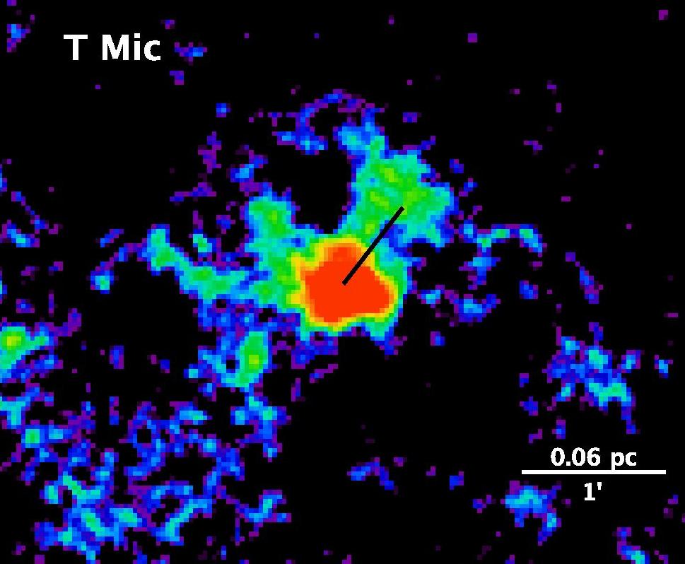
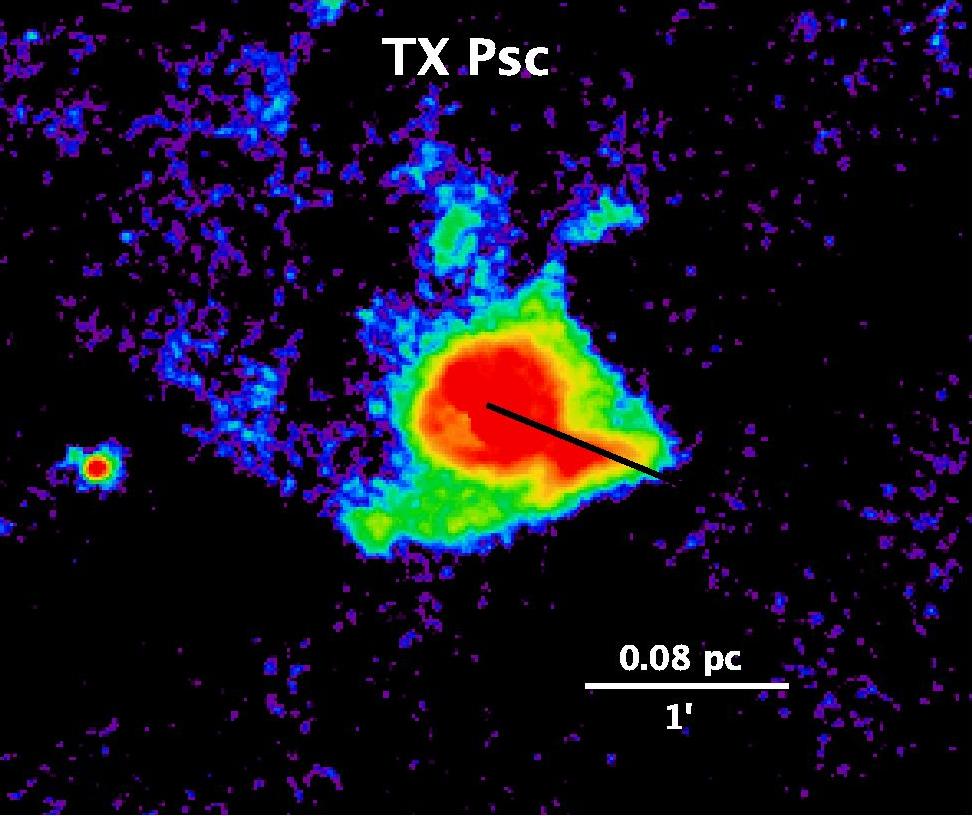
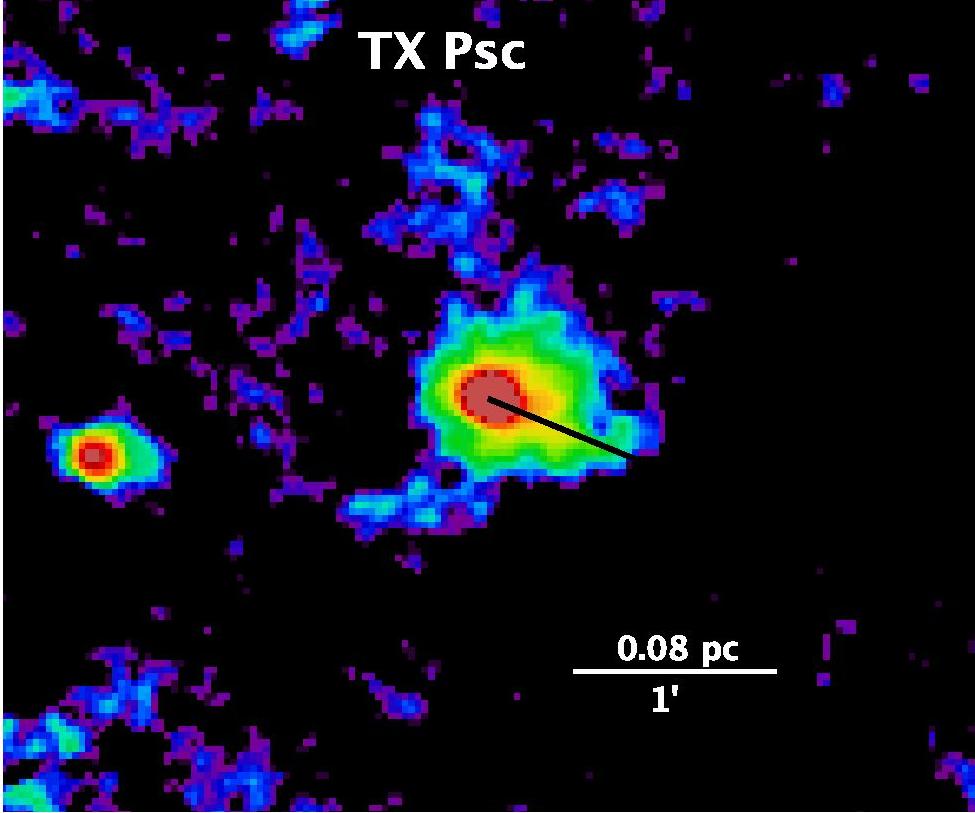
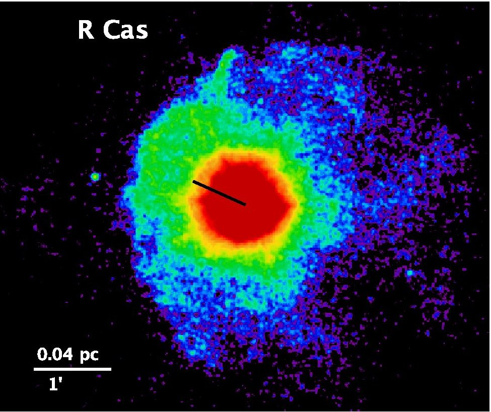
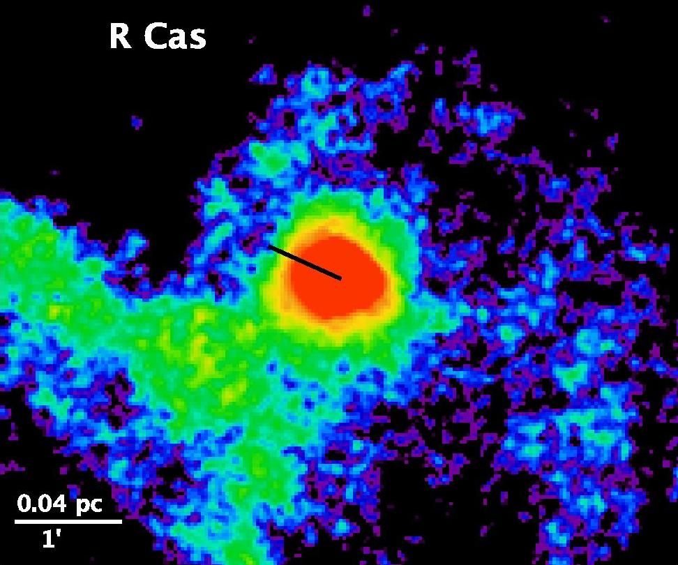
Figure 1: (continued). Interaction type “fermata” (Class I). PACS 70 $\mu$m (left) and 160 $\mu$m (right). V1943 Sgr, T MIrc, TX Psc, and R Cas reveal RT and/or KH instabilities. Note: TX Psc also has an inner spherical shell (not visible here).The sources visible eastward of TX Psc are background galaxies (see also Jorissen et al. 2011).

2 AGB stars and supergiants in the MESS Herschel Key Program

The MESS (Mass-loss of Evolved StarS) program (Groenewegen et al. 2011) is a large far-infrared Herschel (Pilbratt et al. 2010) survey aimed at studying the mass-loss history of evolved stellar objects, from AGB stars to post-AGB, planetary nebulae, luminous blue variables and supernovae. One key goal of the MESS program is to resolve the circumstellar envelopes around a representative sample of evolved stars (from AGB stars to PNe), thereby studying the global evolution of mass-loss and circumstellar envelope structure. The details of the program, the complete target list, data processing approach, and first science results are summarised in Groenewegen et al. (2011).

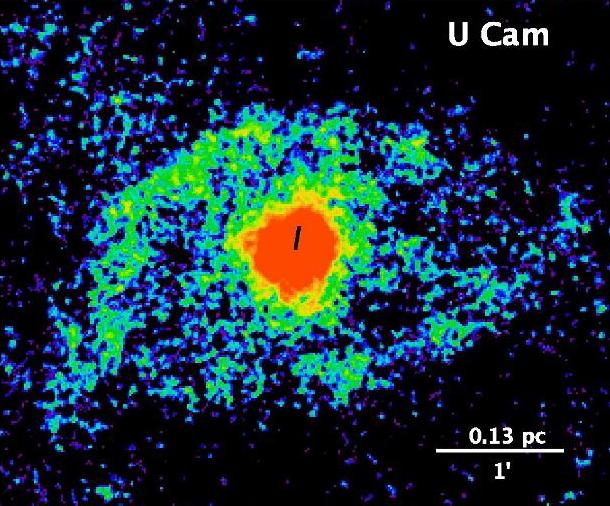
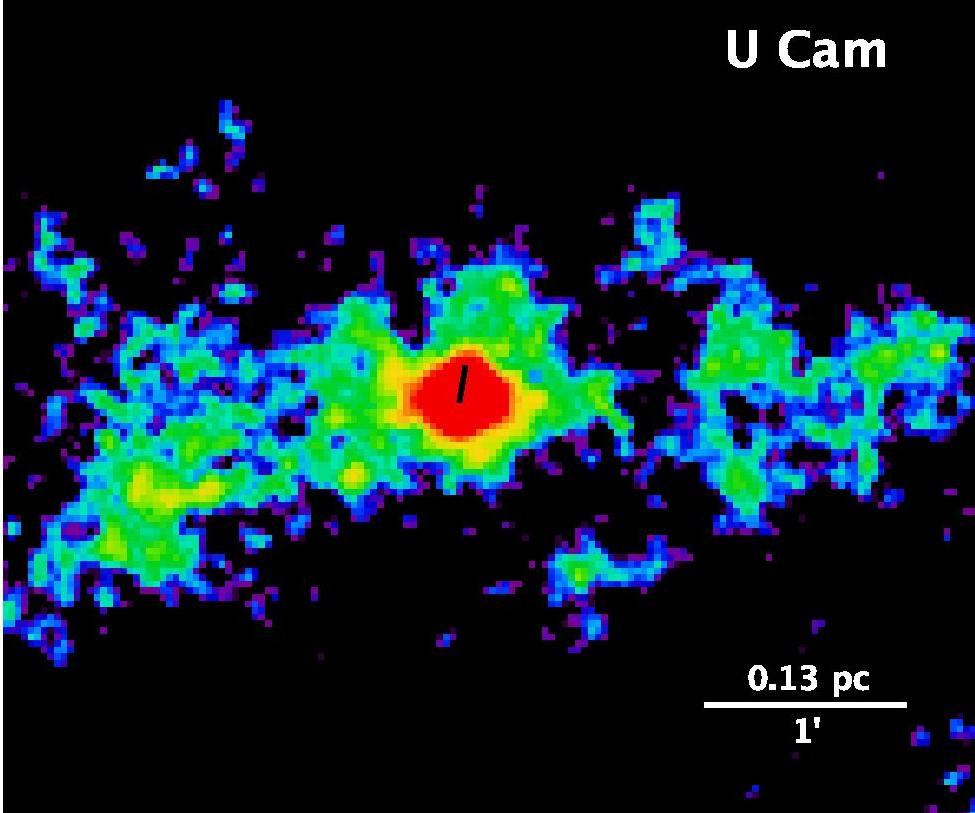
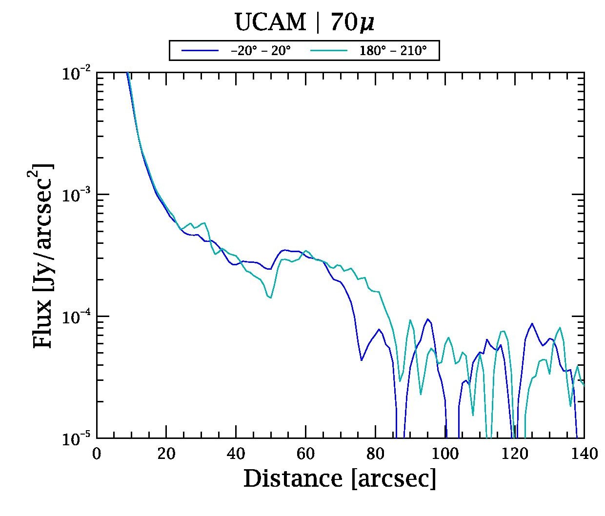
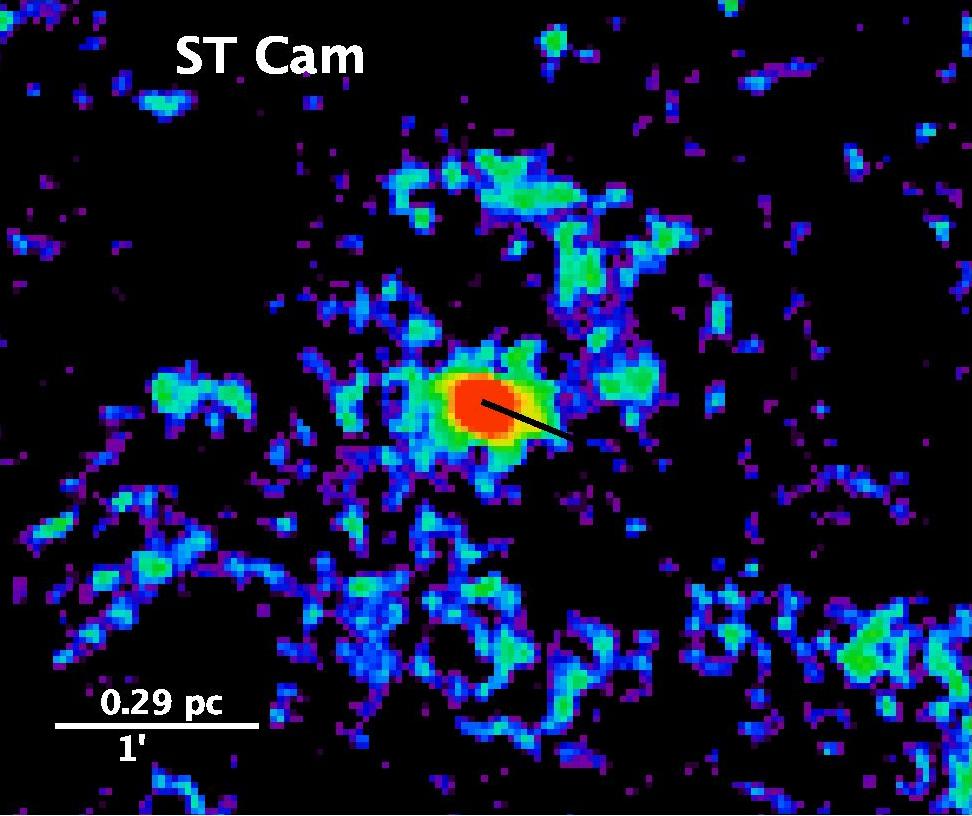
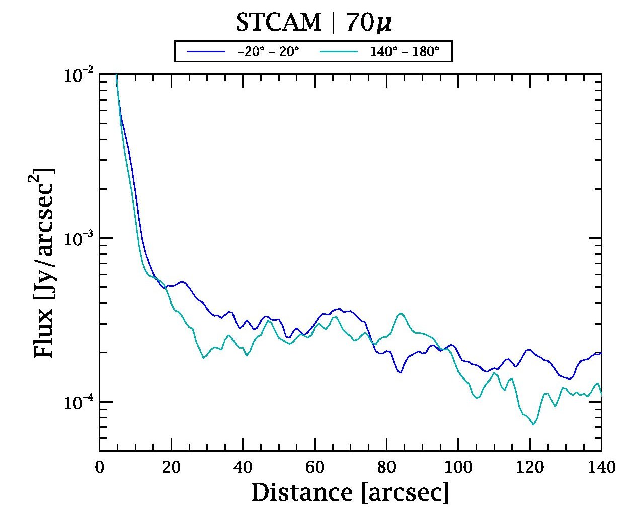
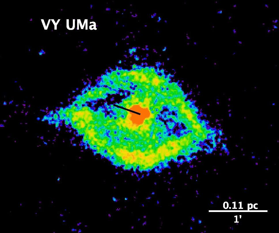
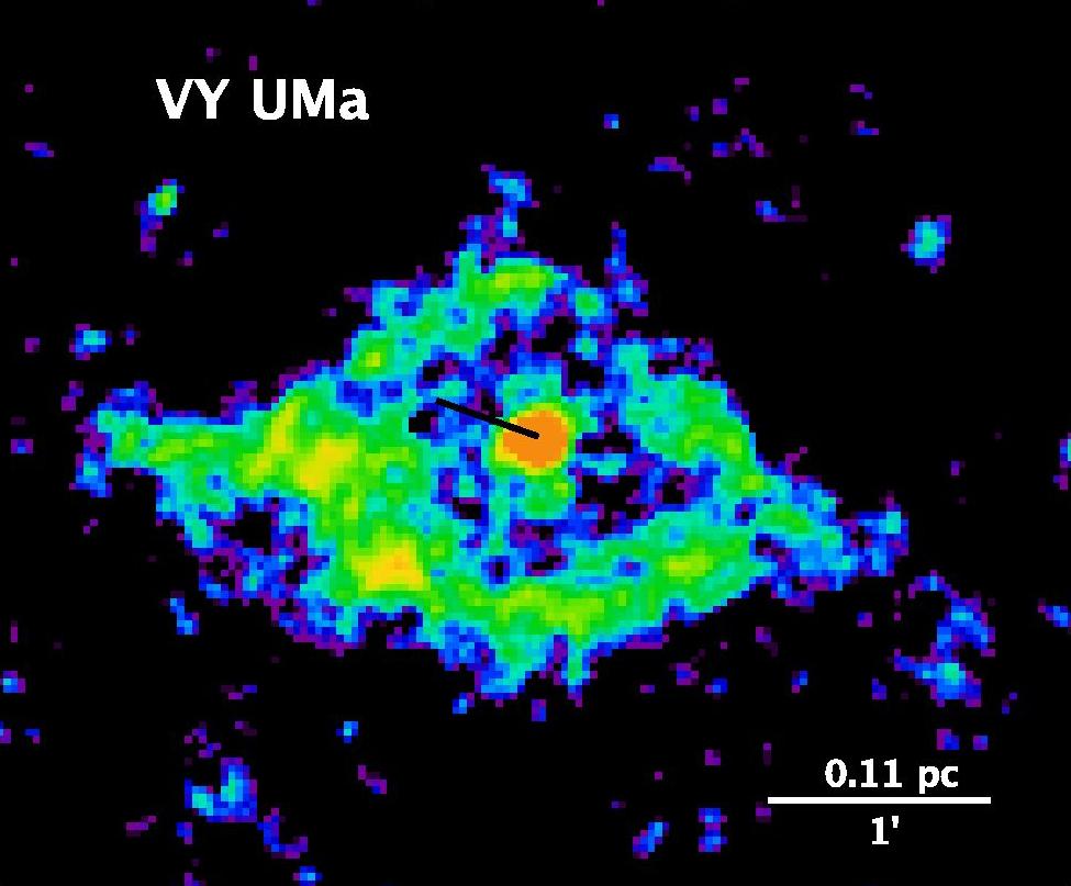
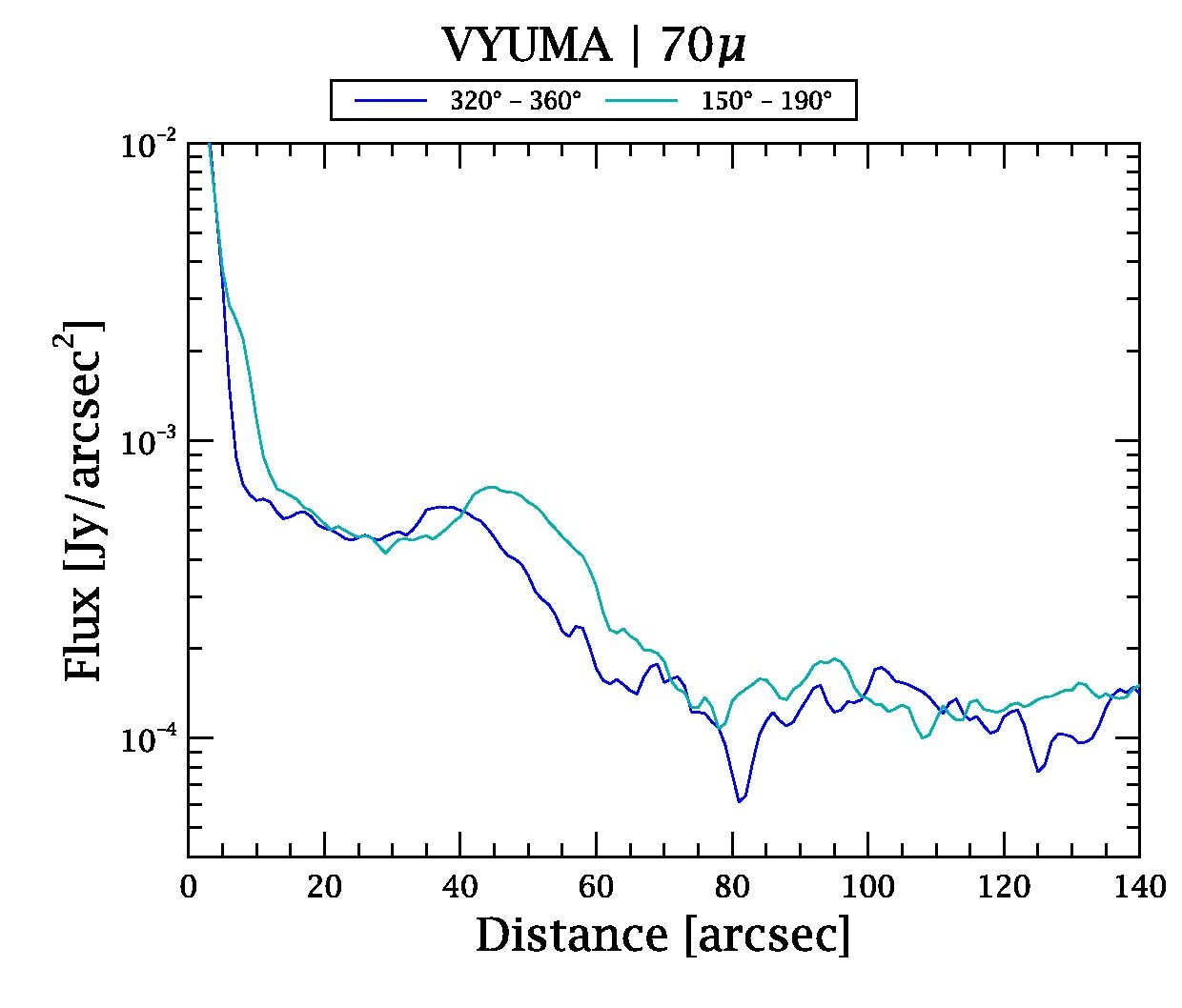
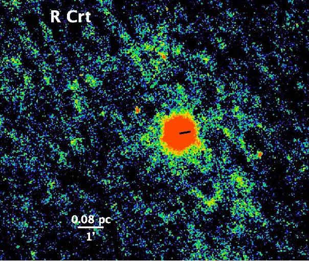
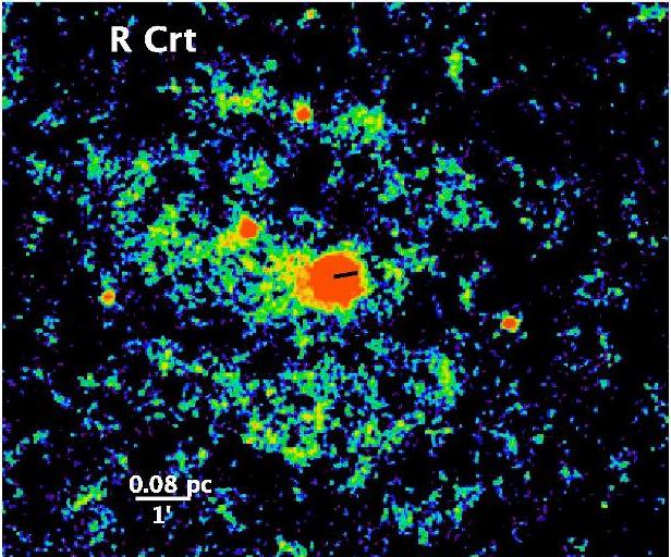
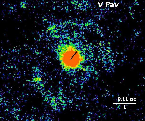
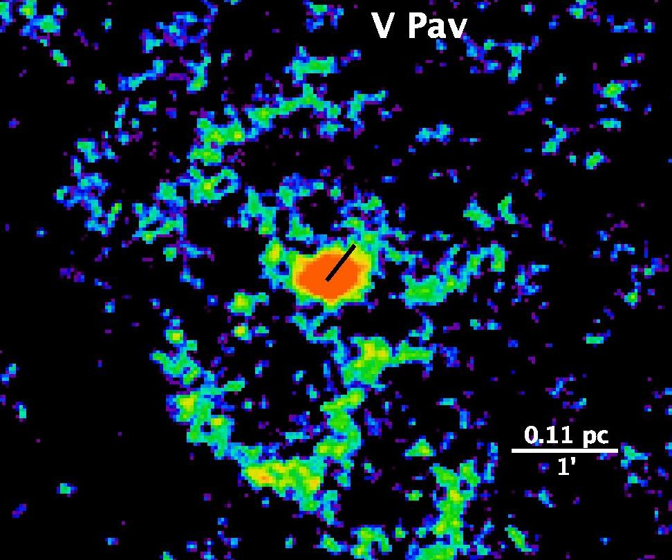
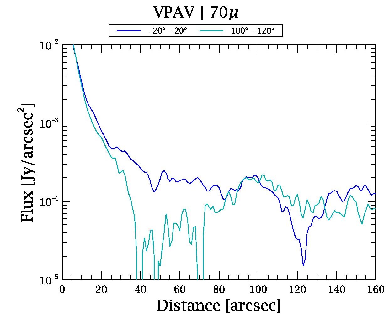
Figure 2: Interaction type “eyes” (Class II). PACS 70 $\mu$m (left) and 160 $\mu$m (middle). Azimuthally averaged radial profiles are shown for 70 and 160 $\mu$m (right). Azimuth opening angles adopted for the radial profile are indicated at the top of each radial profile panel. Note: U Cam also has an inner spherical shell (not visible here).

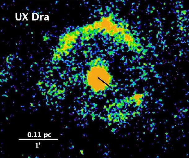
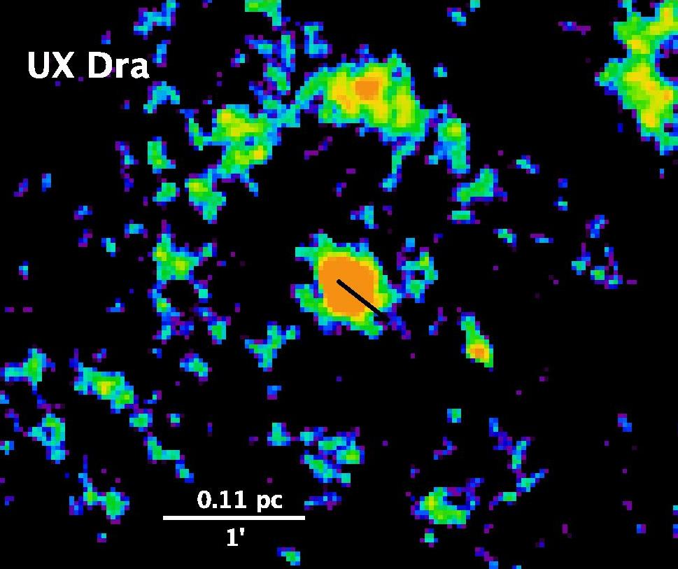
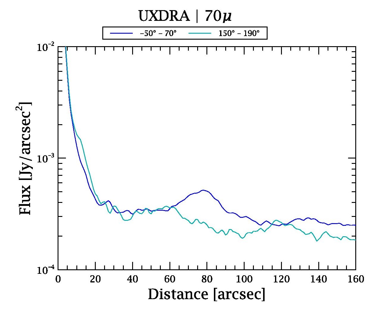
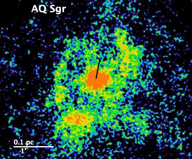
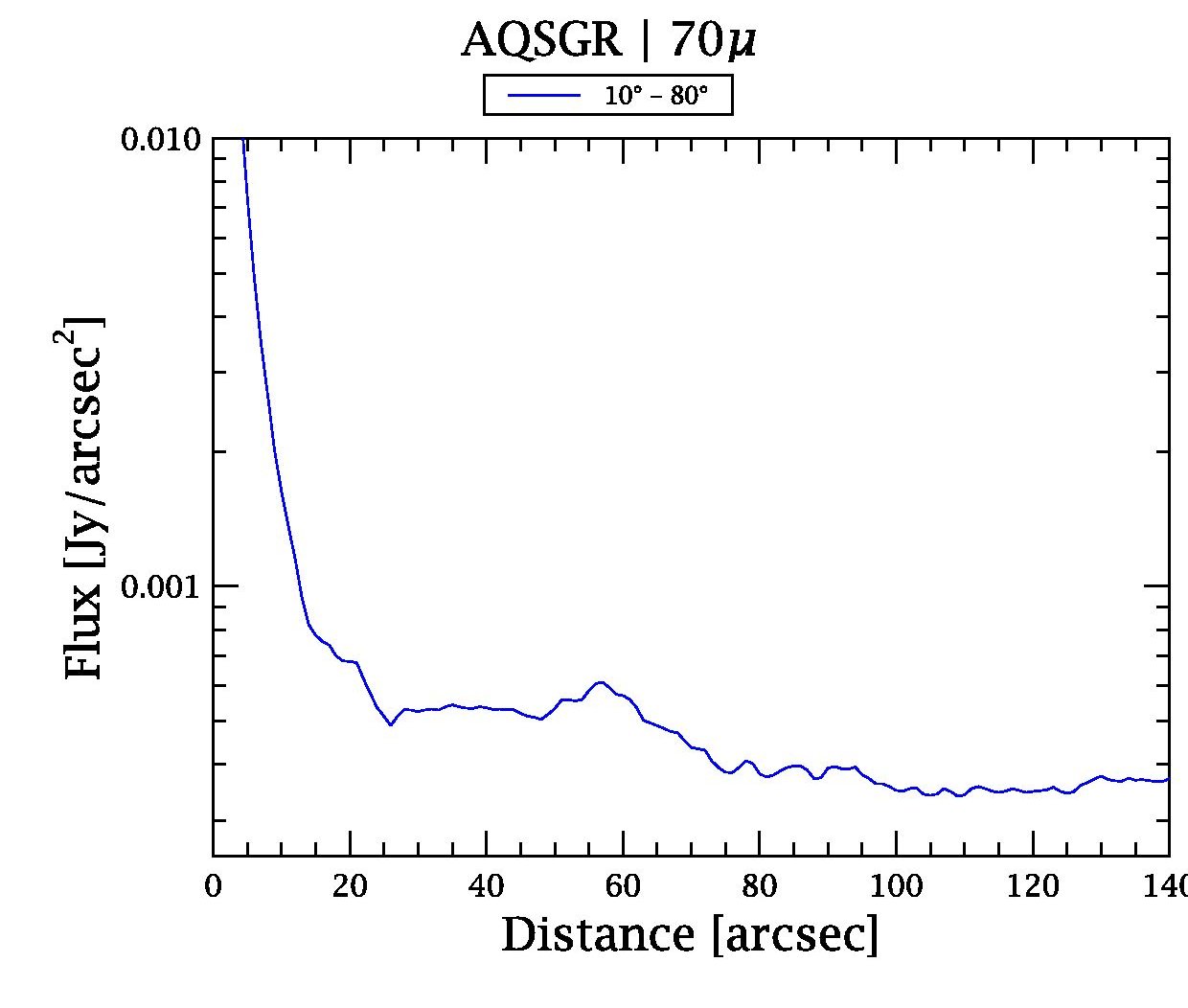
Figure 2: (continued) Interaction type “eyes” (Class II). PACS 70 $\mu$m (left) and 160 $\mu$m (middle). Azimuthally averaged radial profiles are shown for 70 and 160 $\mu$m (right). Azimuth opening angles adopted for the radial profile are indicated at the top of each radial profile panel.

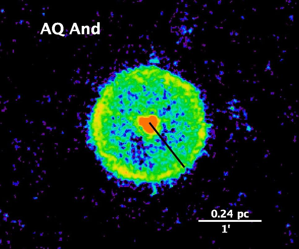
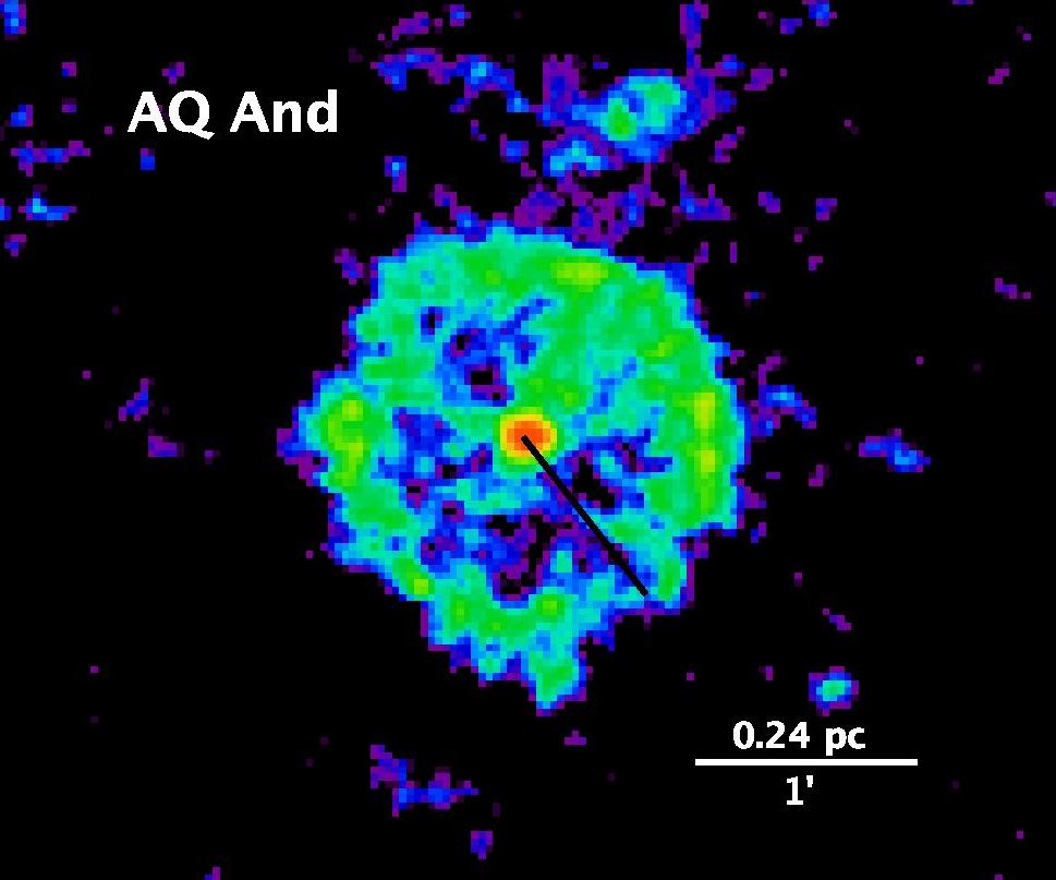
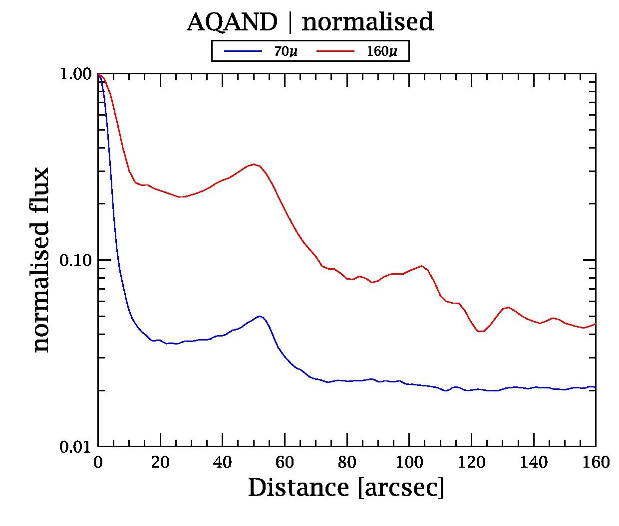
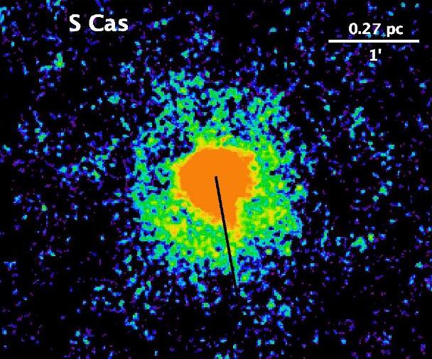
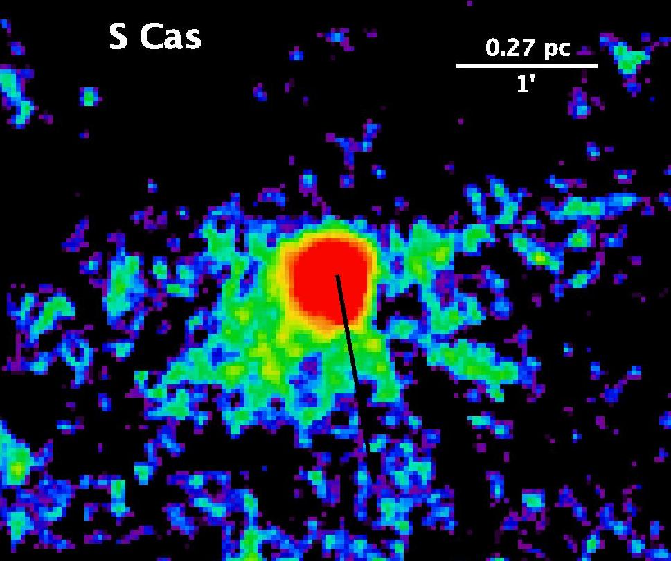
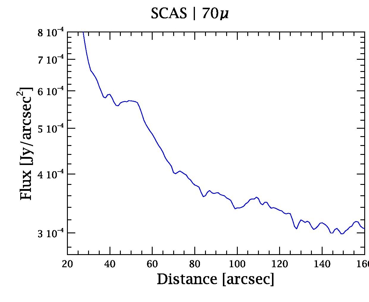
Figure 3: Interaction type “rings” (Class III). PACS 70 $\mu$m (left) and 160 $\mu$m (middle). Azimuthally averaged (360°) radial profiles are shown for 70 and/or 160 $\mu$m (right). The ring towards S Cas is only faintly visible in the current display, but its presence is verified from the radial profiles. For AQ And see also Kerschbaum et al. (2010).

Briefly, infrared scan maps of a large sample of AGB stars and supergiants are obtained with the Photodetector Array Camera and Spectrometer (PACS; Poglitsch et al. 2010) using the “scan map” observing mode with the “medium” (20″ s^-1) scan speed in the blue (70 $\mu$m) and red (160 $\mu$m) filter setting. To create a uniform coverage, avoid striping artefacts, and increase redundancy, two observations at orthogonal scan directions are systematically concatenated. Scan lengths range from 6 to 34′, scan leg steps are 77.5′ or 155′, and repetition factors ranged from 2 to 8.

Data processing was performed applying the standard pipeline steps. In particular, a careful correction of the detector signal drifts is critical to reveal faint extended emission structures with PACS. After deglitching, we applied two different map-making algorithms to assess the quality of the final map, and to verify the faint emission associated to the wind-ISM interaction; these are “PhotProject” with high-pass filter (HIPE v.7.0.) and “Scanamorphos” (Roussel 2011). The maps shown here are those obtained with the latter method as these are less susceptible to the filtering of true extended emission. All frames are projected onto an image with a pixel size of 1″ and 2″ for the blue (70 $\mu$m) and red (160 $\mu$m) bands, respectively. Thus, the final image over-samples the instrumental point-spread functions, which have full-width at half-maxima of 5.6″ and 11.4″ at these wavelengths, respectively.

Aperture photometry of the central point-like sources observed with PACS at 70 and 160 $\mu$m shows that both the “PhotProject” and “Scanamorphos” maps give flux densities that agree within 5%, well within the 15% calibration uncertainties. However, the processing with the updated calibration files in HIPE 7.0 results in 70 and 160 $\mu$m fluxes that are 11% and 15% lower, respectively, compared to the values presented in Groenewegen et al. (2011) using HIPE 4.4.

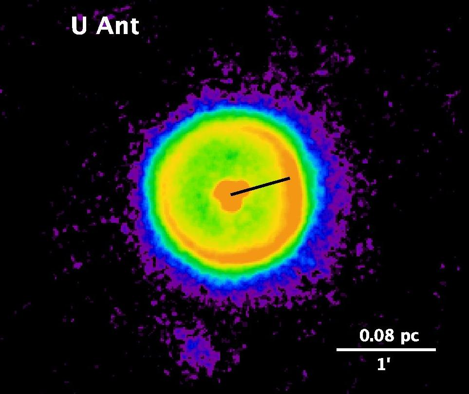
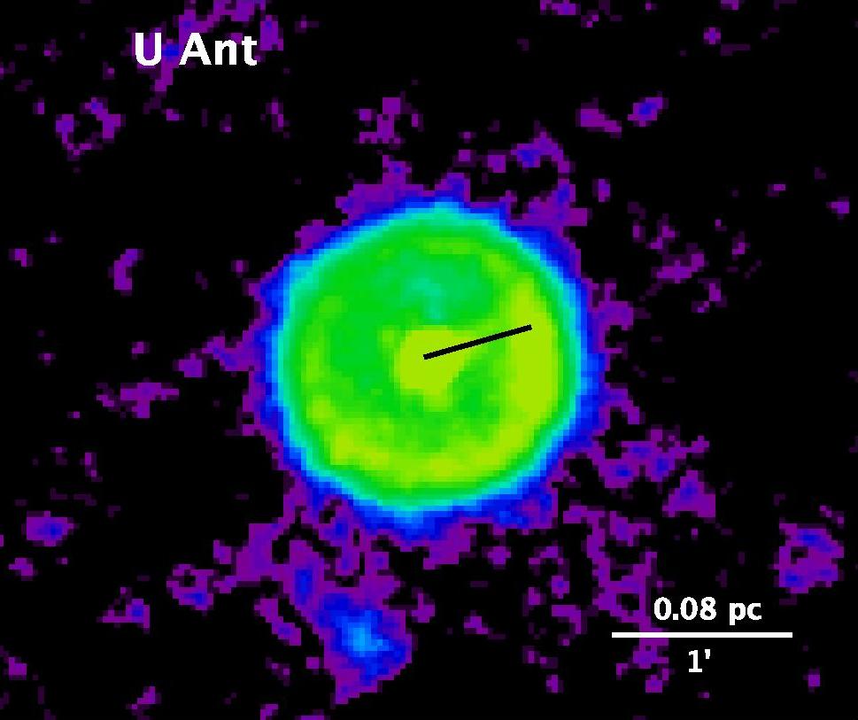
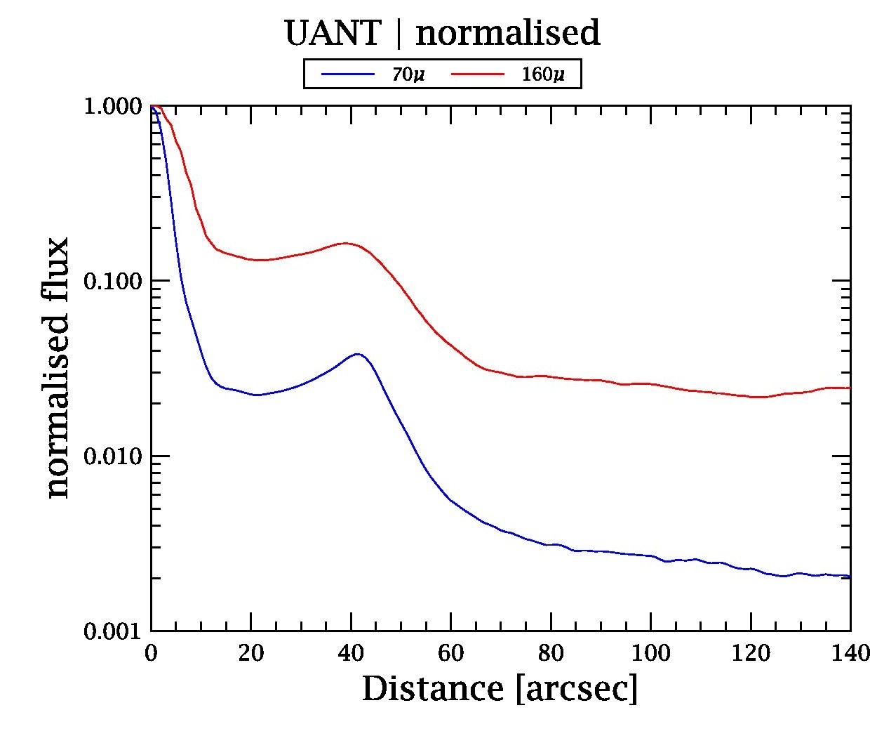
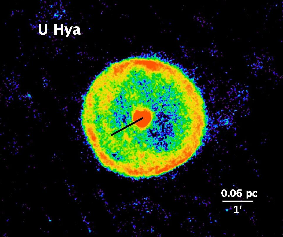
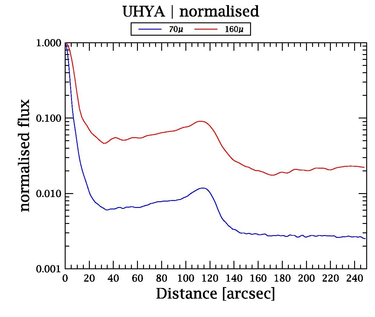
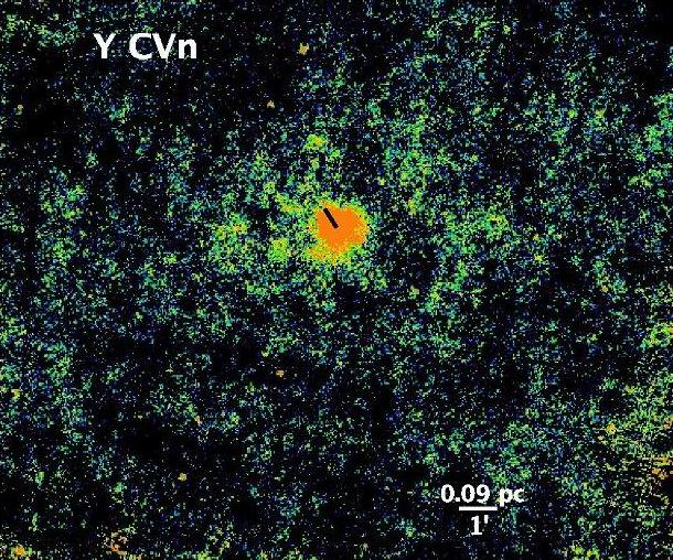
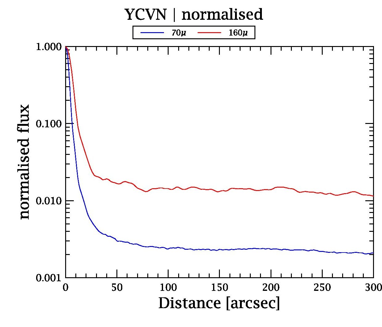
Figure 3: Interaction type “rings” (Class III). PACS 70 $\mu$m (left) and 160 $\mu$m (middle). Azimuthally averaged (360°) radial profiles are shown for 70 and/or 160 $\mu$m (right). For U Ant see also Kerschbaum et al. (2010). The ring towards Y CVn is only faintly visible in the current display, but its presence is verified from the previous detection with IRAS (Izumiura et al. 1996).

Figures 1 to 4 presents the objects in our sample which reveal signs of extended and/or detached dust emission around the central star in either or both the PACS 70 and 160 $\mu$m bands. Colour versions of these figures are available in the electronic edition providing enhanced visibility. The different observed morphologies are divided in several classes (see Sect. 3). Out of 78 AGB stars and supergiants imaged with PACS as part of the MESS survey, 32 stars show clear evidence of wind-ISM interaction, 15 stars show detached rings, and 6 show extended irregular emission (Tables LABEL:tb:properties1 and LABEL:tb:properties1b). The remaining 30 stars do not show evidence for wind-ISM interaction (Table LABEL:tb:properties2). Tables LABEL:tb:properties1 to LABEL:tb:properties2 provide basic properties of the observed AGB stars and supergiants; IRAS identifier (col. 1), Name (col. 2), Distance (col. 3), Mass-loss rate (col. 4), $z$ (col. 5); height above the Galactic plane, $n_{H}$ (col. 6); local ISM density, $\mu$ (col. 7); proper motion, $v_{\star}$ (col. 8); space velocity, P.A. (col. 9); the proper motion position angle measured from north to east, $i$ (col. 10); the inclination angle of the space motion with respect to the plane of the sky, and $v_{w}$ (col. 11) the terminal wind velocity. In addition, we also provide the predicted stand-off distance, $R_{0}$ in arcminutes (col. 12) and parsec (col. 13), as well as, for Tables 1 and 2, the measured stand-off distance $R_{0}$ in arcminutes (col. 14), parsec (col. 15), the position angle $\theta$ (col. 16) and the inferred local ISM density, $n_{H}$ (col. 17). Columns 18 and 19 give information on the spectral type / circumstellar chemistry and binarity, respectively.

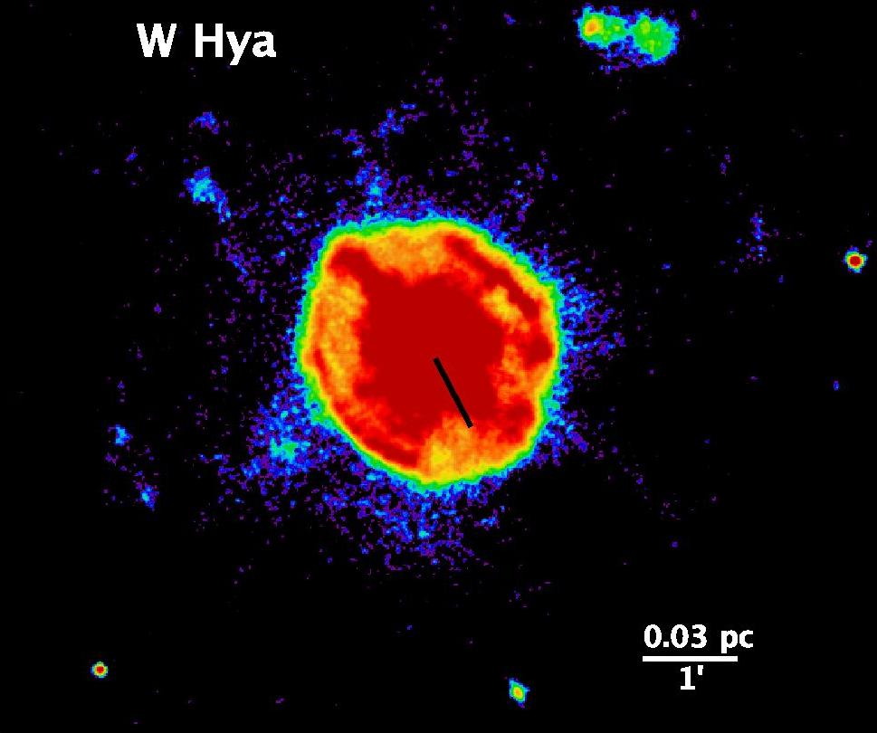
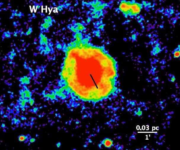
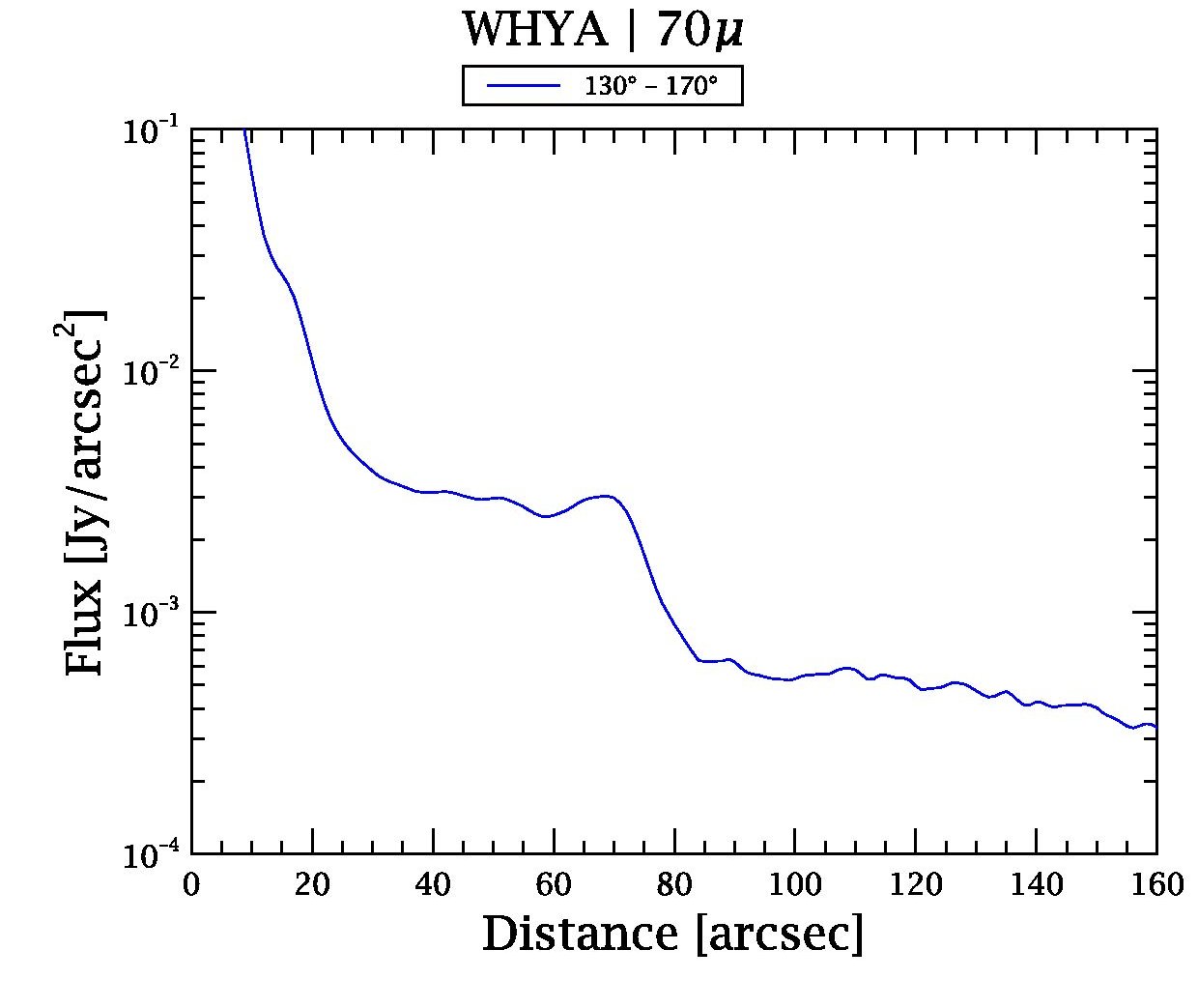
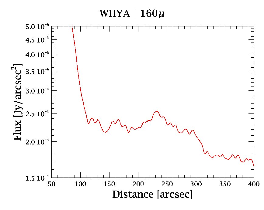
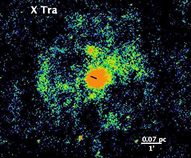
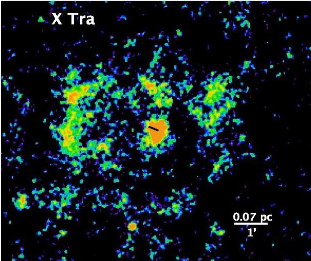
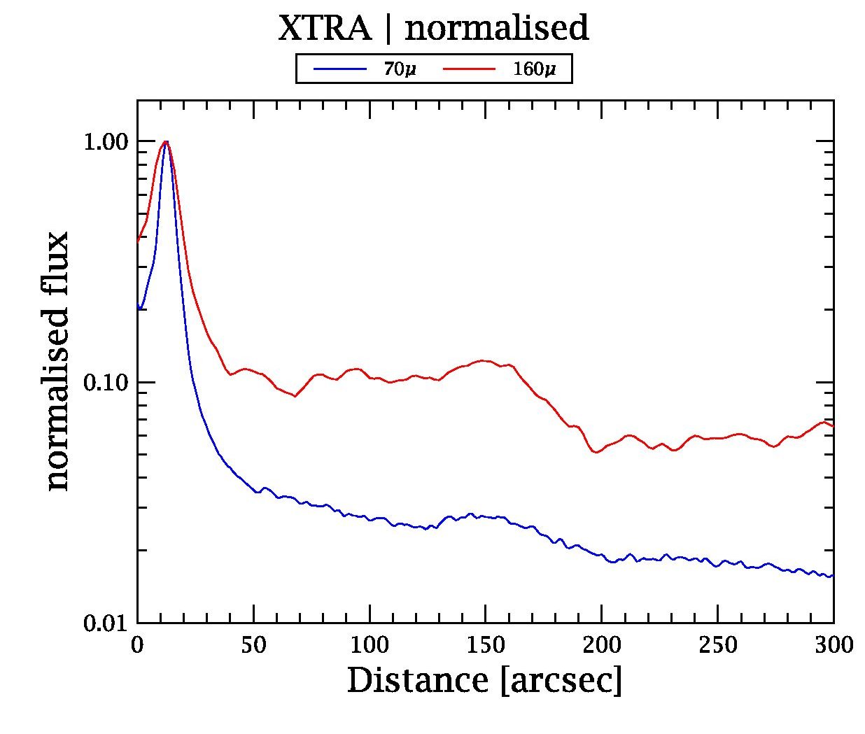
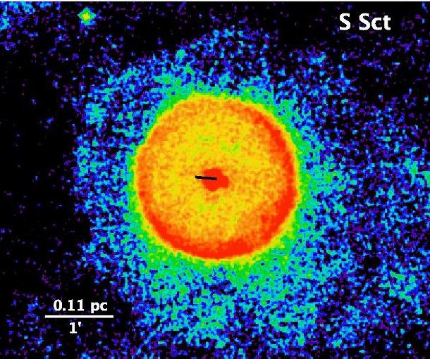
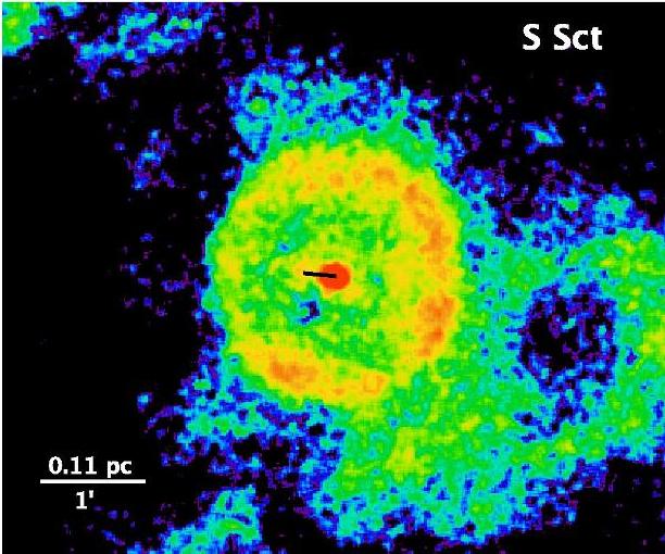
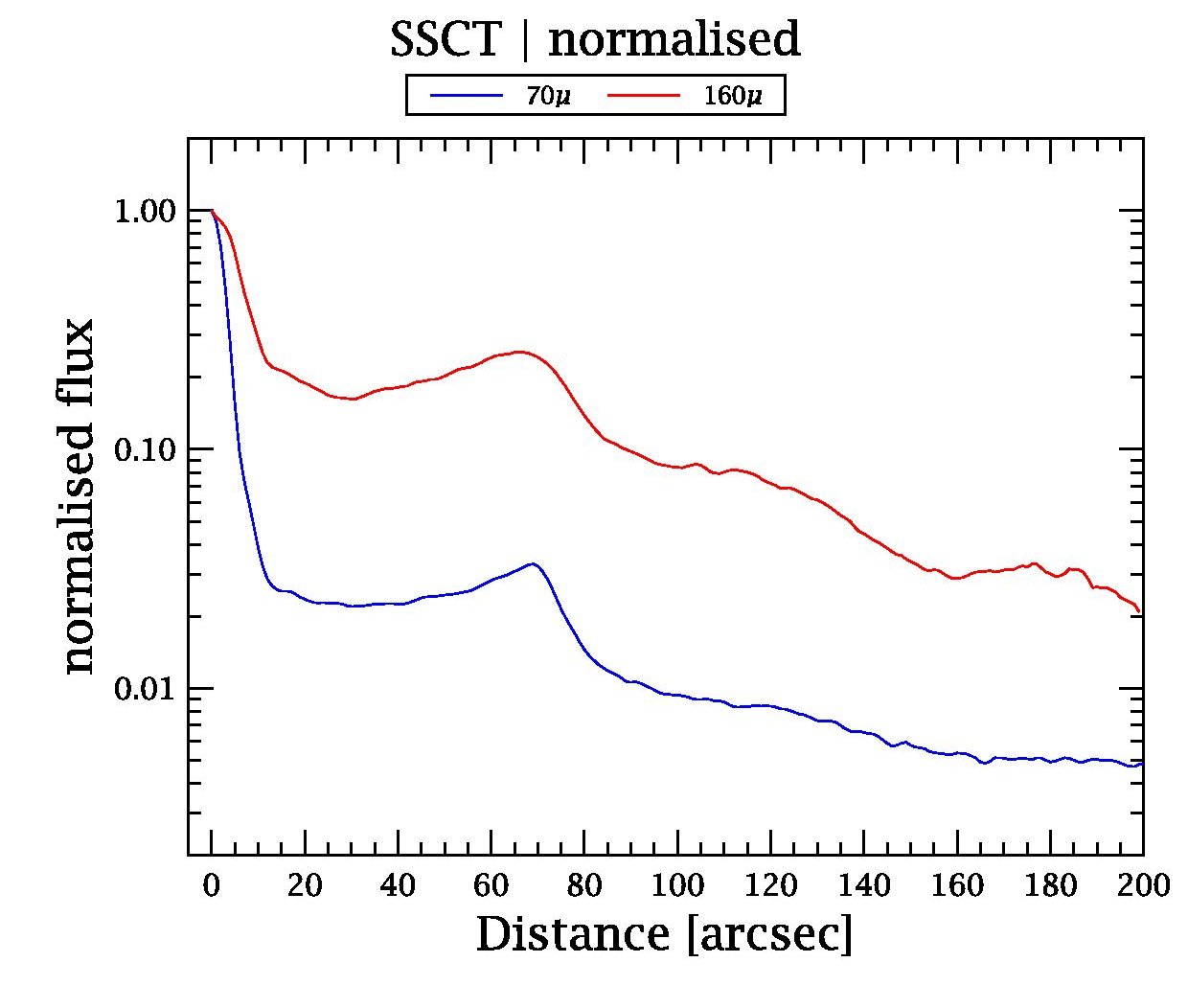
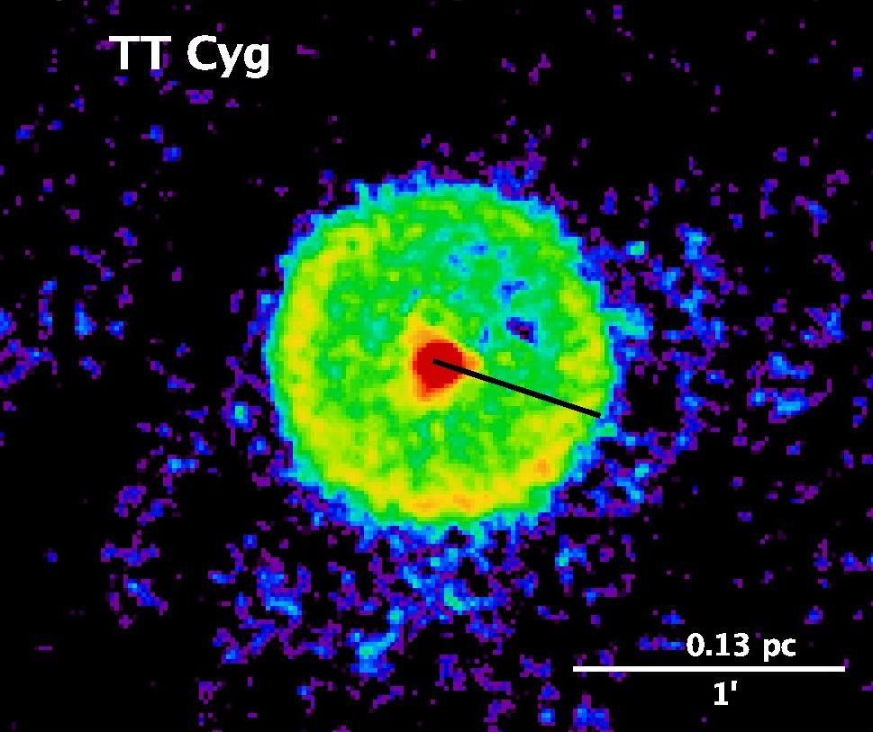
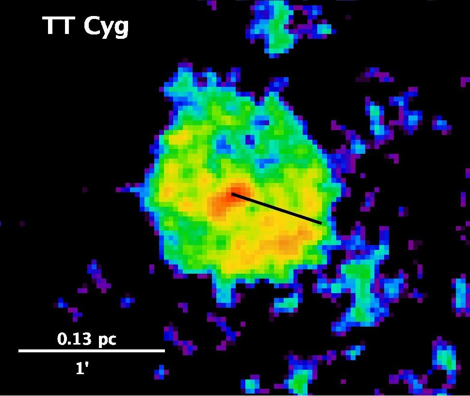
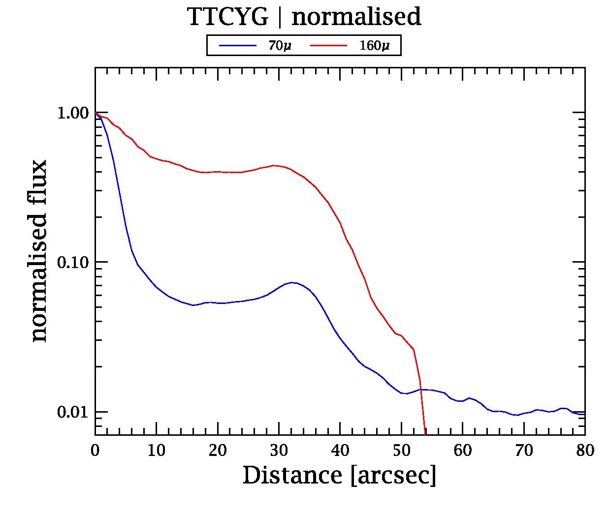
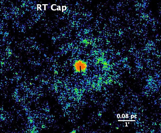
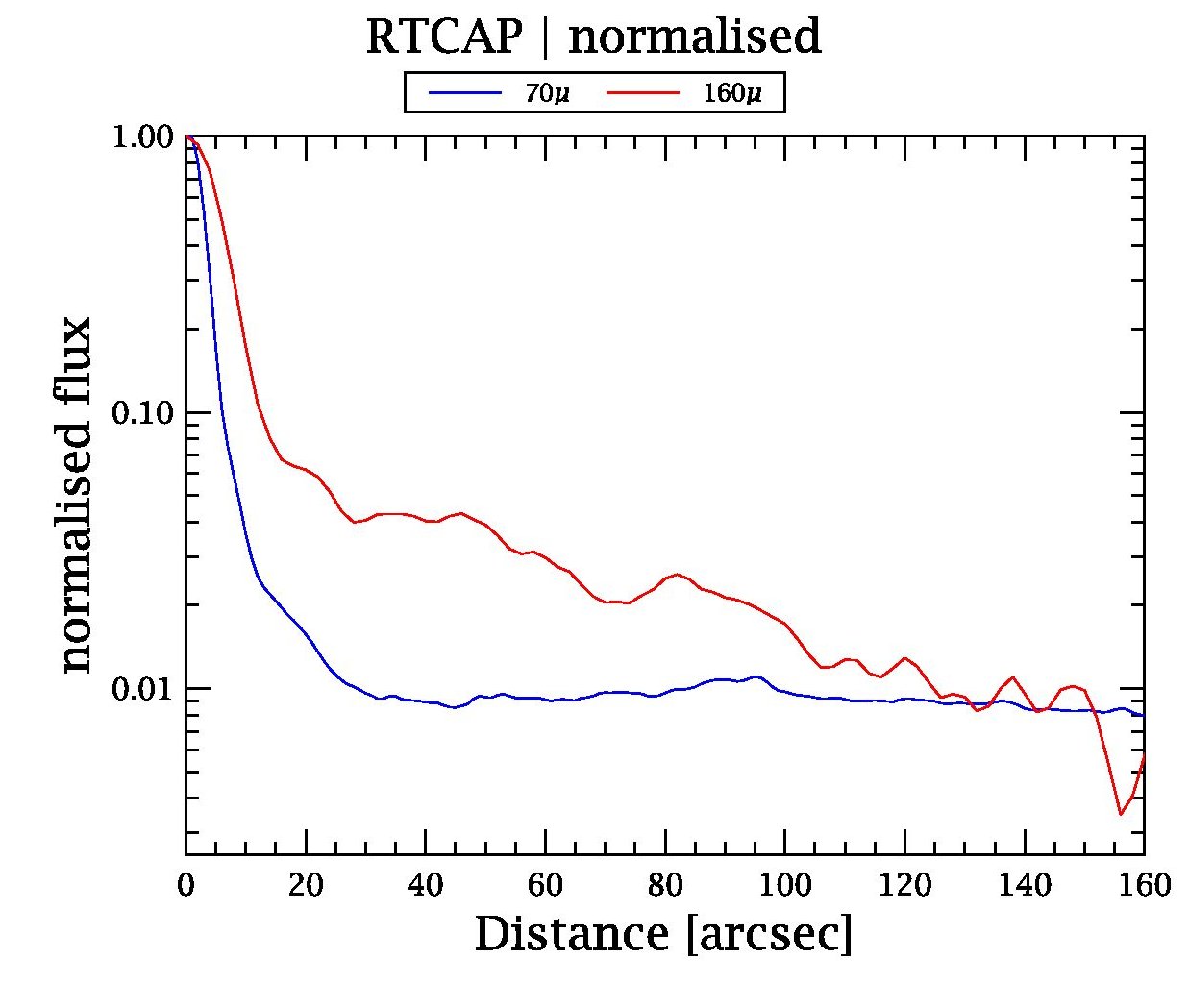
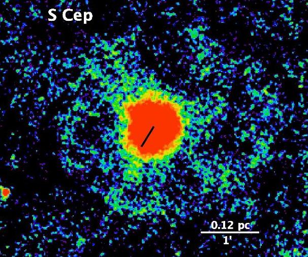
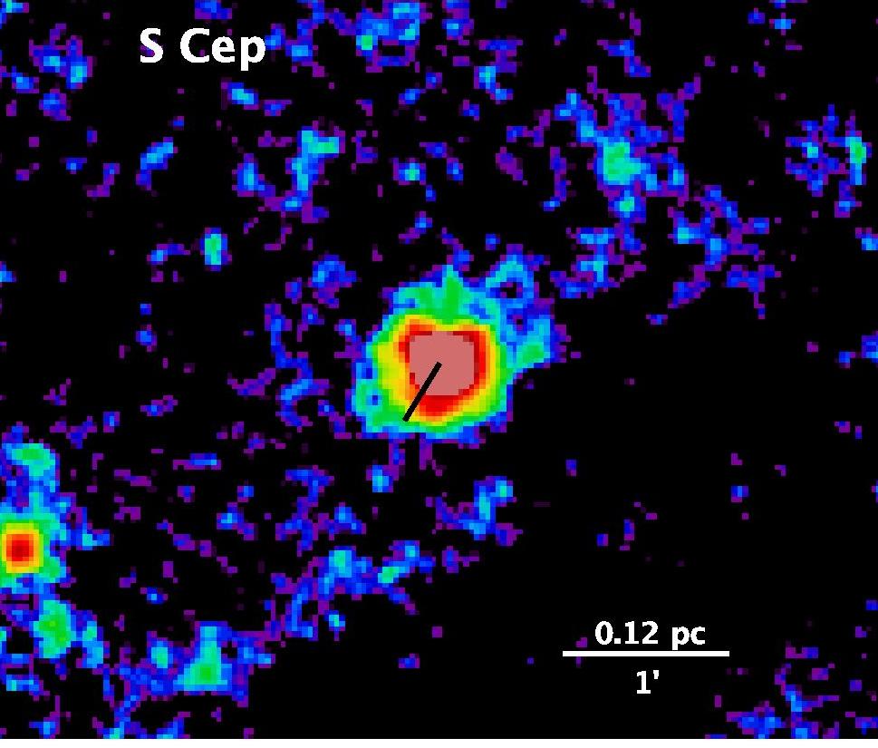
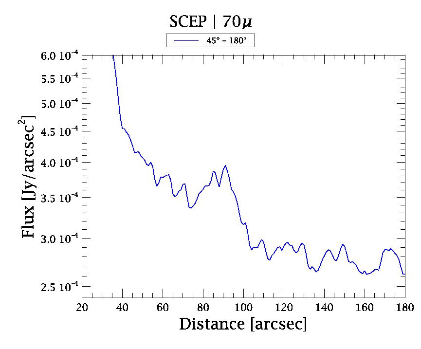
Figure 3: (continued) Interaction type “rings” (Class III). PACS 70 $\mu$m (left) and 160 $\mu$m (middle). Azimuthally averaged (360°) radial profiles are shown for 70 and/or 160 $\mu$m (right). For TT Cyg see also Kerschbaum et al. (2010). The ring around W Hya is incomplete and deviates slightly from sphericity, also a jet-like structure is visible in the north-east direction.

After deconvolution, three stars (R Scl, TX Psc, U Cam) reveal evidence for both a wind-ISM interaction as well as a detached ring. To measure the ring of TX Psc a de-convolved 2D-image was used. Detailed studies of some individual (classes of) objects included in the survey here are being presented in companion papers. The complex multiple wind-ISM interaction shells associated to $\alpha$ Ori are presented, together with complementary observations, in Decin et al. (in preparation). The interaction around X Her and TX Psc is described by Jorissen et al. (2011) and that of $o$ Cet by Mayer et al. (2011). First results on the detached ring-like shells around AQ And, TT Cyg and U Ant were already discussed by Kerschbaum et al. (2010), while CW Leo (IRC+10 216) was discussed previously by Ladjal et al. (2010) and Decin et al. (2011). Also, the objects with both inner shells and large detached bow shock regions will be discussed in more detail in a forthcoming paper. This notwithstanding, these sources are included here to complete the sample of observed AGB stars and red supergiants.

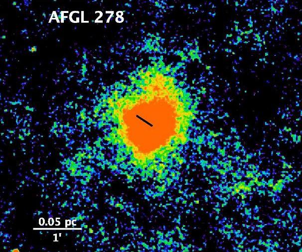
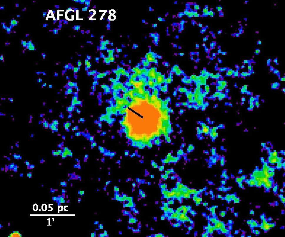
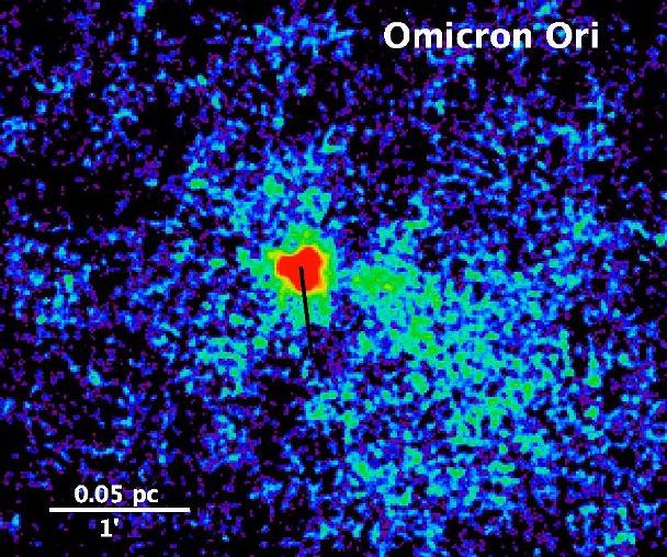
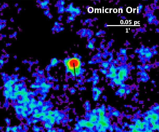
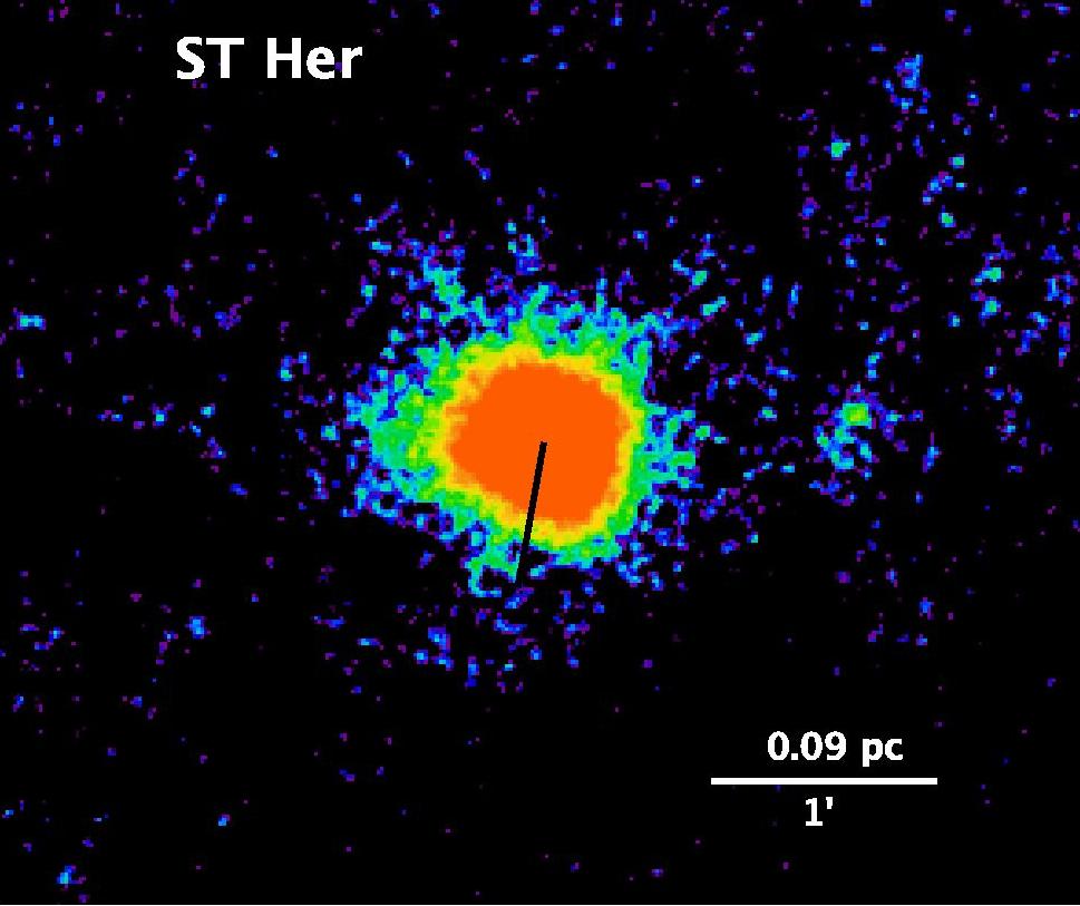
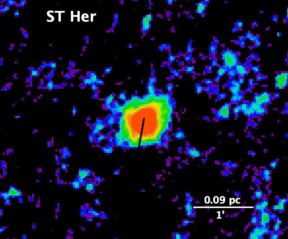
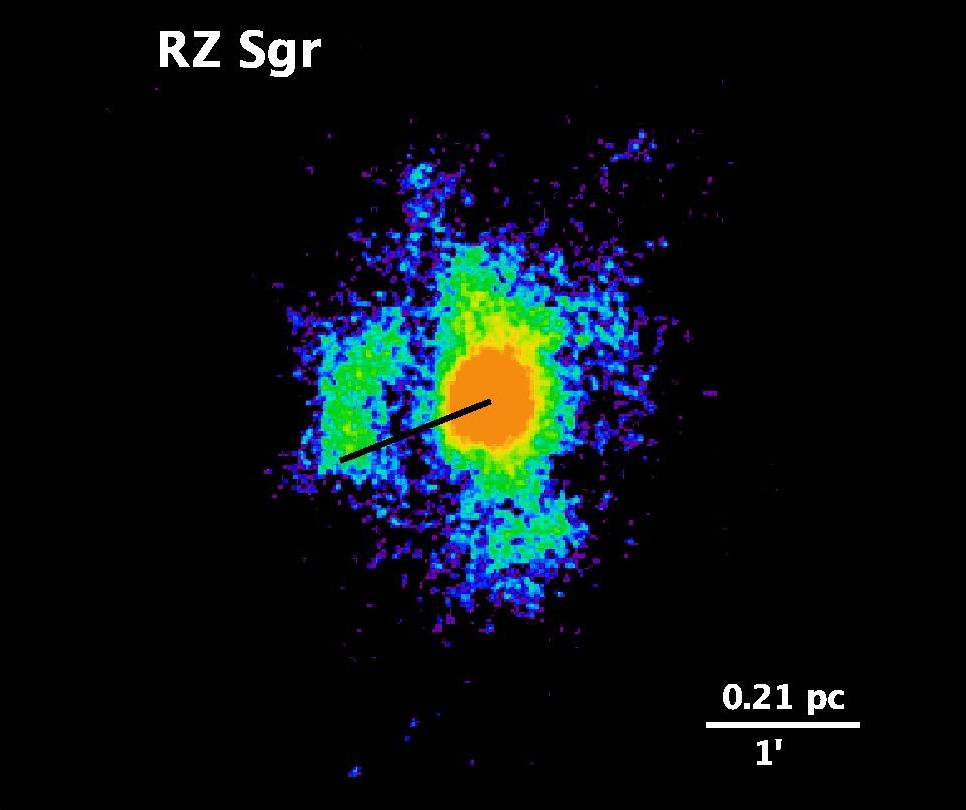
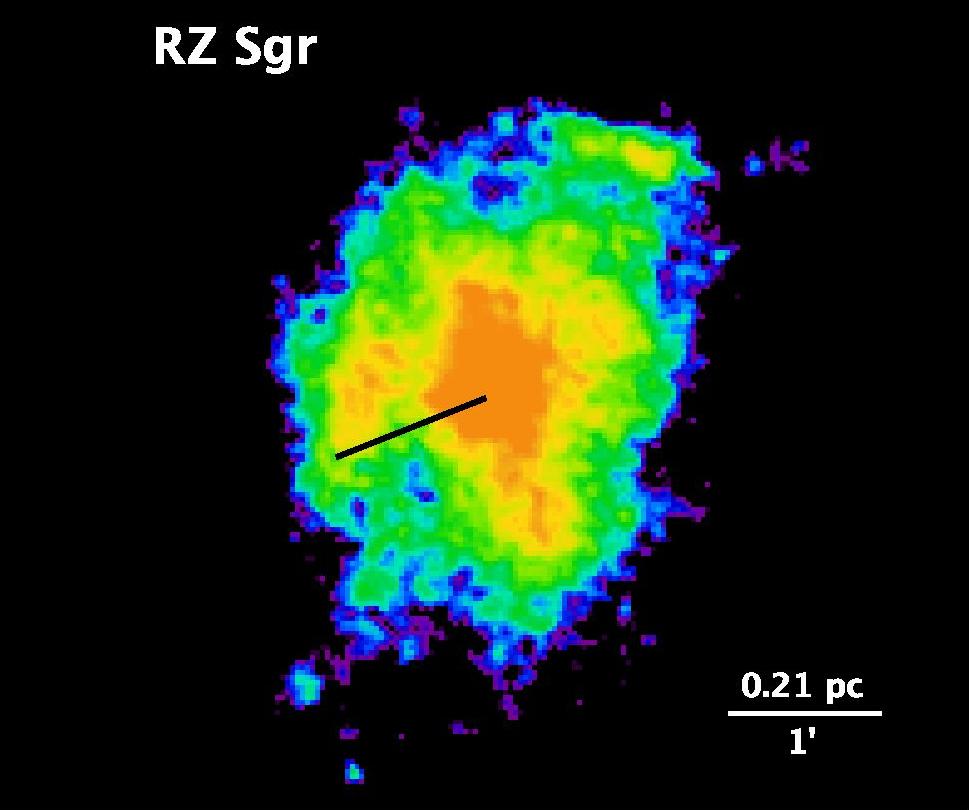
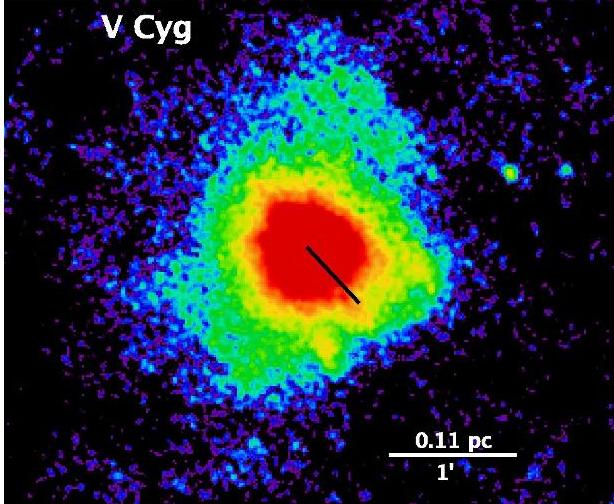
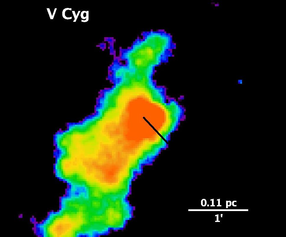
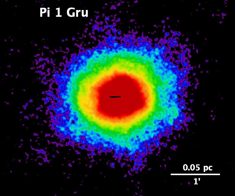
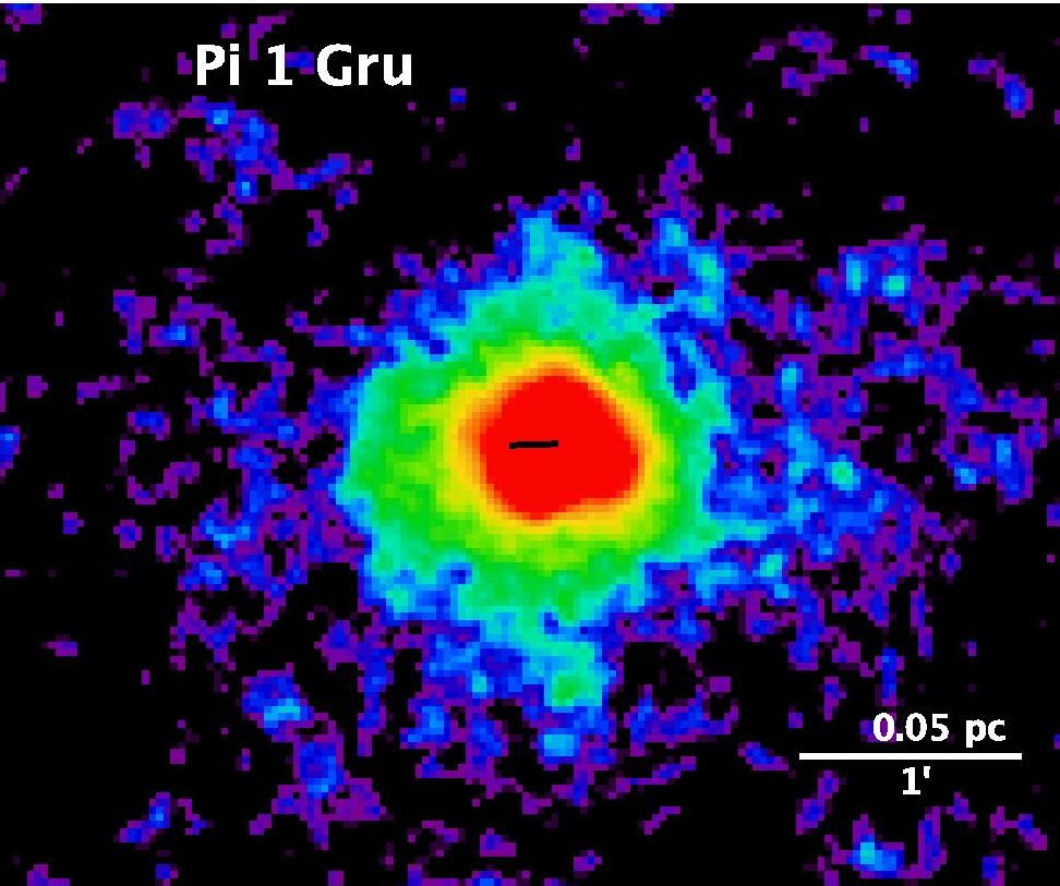
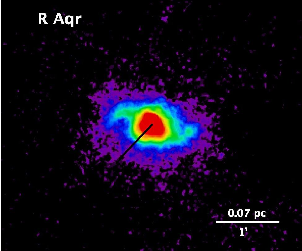
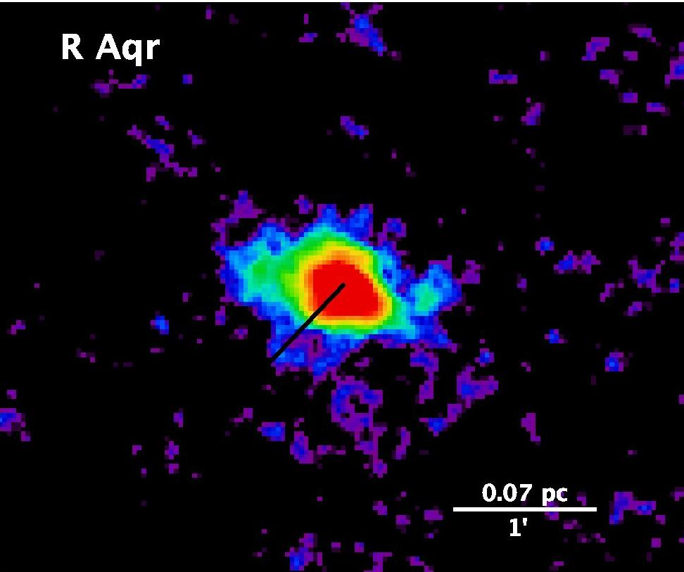
Figure 4: Interaction type “irregular” (Class  IV). PACS 70 $\mu$m (left) and 160 $\mu$m (right). These objects all show some evidence of irregular, diffuse extended emission. However, their morphology is neither a clear (double) arc nor a ring (possibly simply due to observational limitations in sensitivity and/or spatial resolution) and are therefore included in Class IV.

1

Table 1: Key properties of AGB stars and supergiants that show wind-ISM bow shock interaction at 70 $\mu$m and/or 160 $\mu$m. The objects marked with $*$ show a combination of two types of interaction: an inner spherical ring together with an outer extended structure. And, the object with $**$ is either a typical Fermata bow shock or a spherical ring.

IRAS identifier	Name	Distance	$\dot{M}$	$z$	$n_{H}$	$\mu$	$v_{\star}$	P.A.	$i$	$v_{w}$	predicted $R_{0}$			observed $R_{0}$			$n_{H}$	Type	Binary
		(pc)	($10^{-7}M_{\odot}$ yr-1)	(pc)	(cm-3)	(mas yr-1)	(km s-1)	(° N-E)	(°)	(km s-1)	(′)	(pc)		(′)	(pc)	($\theta$)	(cm-3)
I “Fermata”
00248+3518	AQ And ∗	781$\pm$5556, 825	6.57	-360	0.05	13.4	54.1	218	17		1.5	0.37						C
01246-3248	R Scl ∗	3705, 2906	162	-350	0.06	36.7	66.3	208.3	-15	17.02	4.4	0.48		0.88	0.095	225	1.5	C
02168-0312	$o$ Cet	92$\pm$10h, 1105	2.52	-63	1.07	223.3	107.7	185.3	26	8.12	0.7	0.02		1.23	0.033	181	0.4	O - M7IIIe	yes9
03507+1115	NML Tau	2457	321	-113	0.65	–	$>$33.8		-	18.52	$\leq$5.9	$\leq$0.42		$\sim$1.4	0.10		11.6	O - M6me
05028+0106	W Ori∗∗	377$\pm$135h	2.37	-131	0.54	10.5	18.8	91.5	0	8.616	1.4	0.15		0.7	0.077		2.1	C
05418-4628	W Pic	775$\pm$300h 67026, 512	3.015	-246	0.17	12.5	38.2	348	33	7.025 (13.915)	1.2	0.18		0.57	0.085	292	0.8	C
05524+0723	$\alpha$ Ori	153$\pm$19h, 1312	2.12, 313	-5	1.89	38.7	24.3	47.7	8	14.02	7.7	0.29		4.98	0.19	54	4.6	O - M2Iab
06331+3829	UU Aur	341	2.77, 7428	96	0.76	10.4	17.9	170.4	24	11.016	3.3	0.33		1.32	0.131	200	4.9	C	yes1
09448+1139	R Leo	71$\pm$13h, 1005, 822)	0.922	65	1.05	40.4	13.6	112.3	-4	9.02	4.7	0.10		1.25	0.026	117	14.9	O - M8IIIe
09452+1330	CW Leo	1501, 14019, 1202, 11014	162	100	0.74	82.6	53.3	64.5	-29	14.52	4.5	0.16		6.6	0.23	82	0.3	C - C9.5e
10350-1307	U Hya ∗	208$\pm$10h, 1612	(0.921, 2.014),0.492	143	0.48	66.8	71.9	118.5	-26	8.52	0.3	0.02						C
13001+0527	RT Vir	136$\pm$15h	517	141	0.49	61.9	43.9	96.8	24	8.91,(7.817)	2.6	0.10						O - M8III
13269-2301	R Hya	124$\pm$11h, 1305, 1182	1.62	89	0.82	42.9	25.3	313.7	-23	12.52	2.7	0.09		1.55	0.053	284	2.5	O - M7IIIe	yes1
14003-7633	$\theta$ Aps	113$\pm$6h,	1.17	-13	1.75	63.3	34.2	258.8	2	4.516	0.7	0.02		1.25	0.041	297	0.6	O - M6.5III	yes6
16011+4722	X Her	137$\pm$8h	1.511	116	0.62	79.6	91.2	313.9	-53	6.511	0.4	0.01		0.60	0.024	330	0.5	O - M8III
19126-0708	W Aql	6101, 3404	(2515), 1302	-35	1.40	27.6	51.4	65.3	-29	20.02	4.0	0.40		0.8/1.3	0.08/0.13		35	S - S6.6+FV	yes7
19486+3247	$\chi$ Cyg	181$\pm$36h, 1705, 1492	2.42	24	1.58	52.1	37.6	218.3	16	8.52	1.0	0.05		$\sim$6.6	0.29		0.04	S - S6+/1e
20038-2722	V 1943 Sgr	197$\pm$23h	1.317	-77	0.93	34.7	35.2	155.0	-23	5.417	0.6	0.04		1.1	0.06	135	0.3	O - M7III
20075-6005	X Pav	2702	5.22	-133	0.53	21.9	32.6	84.9	-35	11.02	1.9	0.15		0.78	0.061	88	3.2	O - M7III:p
20248-2825	T Mic	211 $\pm$ 45h	0.817	-98	0.75	30.9	39.9	322.2	39	4.817	0.4	0.03						O - M7III
21419+5832	$\mu$ Cep	3908	202	17	1.69	5.1	21.9	216.3	50	35.02	2.8	0.3		0.83	0.094	85	19.3	O - M2Iae
21439-0226	EP Aqr	114 $\pm$ 8h, 1352	3.12, 0.228, 10.029	-70	0.99	31.2	40.2	4.6	-57	11.52	1.8	0.07		0.45	0.018	22	15.8	O - M8IIIvar	yes8
23438+0312	TX Psc ∗	275 $\pm$ 30h	0.9112	-212	0.24	50.2	66.4	247.7	11	10.512	0.3	0.03		0.62	0.050	238	0.2	C - C5-7,2
23558+5106	R Cas	127$\pm$16h, 176${}_{-92}^{+45}$w	4.02, 1228	-8	1.84	63.4	44.0	65.7	35	13.52	1.6	0.06		1.5	0.055	65	2.1	O - M7IIIe	yes1
II “Eyes”
03374+6229	U Cam ∗	4306	107	60	0.66	4.2	9.8	350.4	49	20.621	5.3	0.66		0.95/1.0	0.12/0.13		30	C	yes1,14
04459+6804	ST Cam	4192, 990	4.57	270	0.14	4.9	28.7	247.8	-31	10.525	1.1	0.31		1.1/1.4	0.32/0.40		0.1	C
10416+6740	VY UMa	380$\pm$51h		286	0.12	15.6	28.2	70.5	-1	7.925	1.5	0.16		0.6/0.8	0.07/0.09		0.4	C	yes2
10580-1803	R Crt	261$\pm$65h	6.91, 1.524, 817	173	0.37	15.8	23.8	279.2	28	10.81,17	3.8	0.29		$\sim$2.3	0.18		1.0	O - M7III	yes1
17389-5742	V Pav	370$\pm$73h	3.414	-76	0.89	5.3	24.0	321.7	56	16.025	1.2	0.13		1.6/1.7	0.17/0.18		0.5	C	yes1
19233+7627	UX Dra	386$\pm$43h	1.6${}^{h},r$	176	0.36	13.0	26.7	231.9	34	4.015	0.7	0.08		1.3/0.9	0.15/0.10		0.2	C	yes4
19314-1629	AQ Sgr	333$\pm$74h	2.515	-81	0.85	8.0	29.1	349.4	66	10.015	0.8	0.08		0.95	0.09		0.6	C
(1) Knapp et al. (1998); (2) De Beck et al. (2010); (3) Harper & Brown (2006); (4) Guandalini & Busso (2008); (5) Whitelock et al. (2008); (6) Knapp et al. (2003); (7) this work (Sect. 5); (8) Raga & Cantó (2008); (9) Ryde et al. (2000); (10) Olofsson (1996); (11) González Delgado et al. (2003); (12) Olofsson et al. (1993); (13) Groenewegen & Whitelock 1996; Groenewegen & de Jong 1998); (14) Groenewegen et al. (2002). Updated distances (van Leeuwen 2007) have been taken to re-scale the (gas) mass-loss rates; (15) Ramstedt et al. (2006); (16) Schöier & Olofsson (2001); (17) Olofsson et al. (2002); (18) Harper et al. (2001); (19) Menzies et al. (2006); (20) Vlemmings et al. (2003); (21) Linquist et al. (1999); (22) Olofsson et al. (2000); (23) Lombaert et al. (in prep); (24) via Period-$\dot{M}$ relation; (25) Loup et al. (1993); (26) Bergeat & Chevallier (2005); (27) Choi et al. (2008); (28) Matthews & Reid (2007); (29) Winters et al. (2003).
Binarity: (1) visual binary, Proust et al. (1981); (2) hot companion, Sahai et al. (2008); (3) symbiotic Mira, Willson et al. (1981); Hollis et al. (1997); (4) suspected by Vetesnik (1984), but could be RV Tau variable instead (Polyakova 1998); (5) white dwarf companion; Ake & Johnson (1988); (6) Makarov & Kaplan (2005); (7) composite spectrum; Herbig (1965); (8) composite CO line; Knapp et al. (1998); (9) visual binary, Prieur et al. (2002); proper-motion binary, Makarov & Kaplan (2005); Frankowski et al. (2007); (10) composite spectrum, Feast (1953); orbital motion, Sahai (1992); proper-motion binary, Makarov & Kaplan (2005); Frankowski et al. (2007); (11) eclipsing system, Knapp et al. (1999); hot companion, Sahai et al. (2008); visual binary, Proust et al. (1981); (12) spiral arm indicative of binary, Mauron & Huggins (2006); (13) spiral arm indicative of binary, Castro-Carrizo et al. (2010); (14) The Hipparcos Double Star solution (position angle is 79°, and separation of 0.17″) gives additional evidence for a close companion, and potential a triple system (if the other visual companion is at 208″ (Alain Jorissen; private communication); (15) Pourbaix et al. (2003) found it to be a ’variability-induced mover’ in the Hipparcos catalogue which is a strong indication for a close visual companion.

Table 1: Notes and references

2

Table 2: Key properties of AGB stars and supergiants with detached rings (Class III) or irregular extended (Class IV) emission at 70 $\mu$m and/or 160 $\mu$m. Notes and references as in Table 1. ^∗ These objects show a combination of two types of interaction: an inner spherical ring together with an outer extended structure. ^∗∗ Either typical Fermata bow shock or a spherical ring.

IRAS identifier	Name	Distance	$\dot{M}$	$z$	$n_{H}$	$\mu$	$v_{\star}$	P.A.	$i$	$v_{w}$	predicted $R_{0}$			observed $R_{0}$			$n_{H}$	Type	Binary
		(pc)	($10^{-7}M_{\odot}$ yr-1)	(pc)	(cm-3)	(mas yr-1)	(km s-1)	(° N-E)	(°)	(km s-1)	(′)	(pc)		(′)	(pc)	($\theta$)	(cm-3)
III “Rings”
00248+3518	AQ And ∗	781$\pm$5556, 825	6.57	-360	0.05	13.4	54.1	218.0	17		1.5	0.37		0.87	0.21	–	0.2	C
01159+7220	S Cas	943	2215	176	0.34	19.4	91.0	190.1	-15	22.013	0.7	0.20		0.83	0.23	–	0.25	O - S
01246-3248	R Scl ∗	3705	(8010), 162	-350	0.06	36.7	66.3	208.3	-15	17.02	4.4	0.48		0.23	0.025	–	22.5	C
03374+6229	U Cam	4306	107	60	1.10	4.2	9.8	350.4	49	20.621	5.3	0.66		0.12	0.015	–	30	C	yes1,14
05028+0106	W Ori ∗	377$\pm$135h	2.37	-131	0.51	10.5	18.8	91.5	0	8.616	1.4	0.15		0.7	0.077	–	2.1	C
10329-3918	U Ant	268$\pm$39h, 2606	(7.67), 4010	90	0.82	19.3	36.5	285.8	41	20.52	5.3	0.41		1.5	0.12	–	10.0	C
10350-1307	U Hya ∗	208$\pm$10h, 1612	(0.921, 2.014), 0.49 2	143	0.48	66.8	71.9	118.5	-26	8.52	0.3	0.02		1.9	0.12	–	0.01	C
12427+4542	Y CVn	321$\pm$35h	1.514	319	0.08	17.2	32.7	32.2	40	7.52	1.8	0.17		3.2	0.30	–	0.03	C
13462-2807	W Hya	104$\pm$12h	0.782	72	0.98	43.9	48.2	207.6	58	8.52, (6.517)	0.8	0.03		1.1/3.8	0.033/0.12	–	0.6	O - M7e	yes1
15094-6953	X TrA	360$\pm$57h, 243	1.316	-29	1.49	14.2	16.4	68.2	-7	8.716	1.1	0.08		2.5	0.18	–	0.3	C
18476-0758	S Sct	386$\pm$85h	1.4x	-8	1.85	5.4	17.5	84.9	59	8.02, (17.310)	0.6	0.07						C	yes1
19390+3229	TT Cyg	436, 6106	(1.17), 5010	52	1.19	9.4	38.3	251.8	-52	12.622	2.2	0.28		0.55	0.070	–	19.7	C	yes1
20141-2128	RT Cap ∗∗	291$\pm$52h	(1.016), 9.47	-121	0.60	5.2	21.6	184.5	-69	8.016	2.9	0.25		1.5	0.13	–	2.2	C
21358+7823	S Cep	407$\pm$107h	1516)	150	0.45	3.2	23.1	148.5	-56	22.016	5.4	0.64		1.5	0.18	–	5.8	C
23438+0312	TX Psc ∗	275$\pm$30h	0.9112	-212	0.24	50.2	66.4	247.7	11	10.512	0.3	0.03		0.27	0.022	–	1.0	C - C5-7,2
IV “Irregular”
01556+4511	AFGL 278	174$\pm$24h		-33	1.44	27.1	22.3	56.7	5	8.325	0.6	0.03						O - M7III
04497+1410	$o$ Ori	200$\pm$28h, 163	$<$ 0.413	-36	1.39	41.1	38.8	187.0	-34		1.9	0.09						O - M3 S	yes5
15492+4837	ST Her	293$\pm$51h	1.315	238	0.19	27.2	38.4	169.8	-7	(9.113), 8.515	1.1	0.09						O - M6-7IIIa S
20120-4433	RZ Sgr	7302	(15015), 5.82	-384	0.04	16.2	63.2	111.6	-28	9.02, (11.413)	1.2	0.26		2.	0.43	–	0.02	S - S4,4
20396+4757	V Cyg	4205, 2712, 366	(9.41), 42	39	1.35	19.4	35.6	223.1	25	15.02	0.8	0.09						C - C5,3
22196-4612	$\pi^{1}$ Gru	163$\pm$20h, 1522	8.52	-119	0.61	8.4	11.9	91.8	-68	30.02	17.1	0.81						S - S5+G0V	yes10
23412-1533	R Aqr	25013, 19728	0.6(28)	-220	0.22	27.5	45.0	136.4	-43	16.714	0.5	0.05						O-M7IIIpev	yes3

Table 2: continued.

3

Table 3: AGB stars that show no obvious bow shocks are assigned to Class X pending further notice. Notes and references as in Table 1. Note that Y Lyn, SW Vir, and AFGL 5379 are classified X pending planned observations.

IRAS identifier	Name	distance	$\dot{M}$	$z^{23}$	$n_{H}^{D}$	$\mu$	$v_{\star}$	P.A.	$i$	$v_{w}^{13}$	predicted $R_{0}^{B}$		Type	Binary
		(pc)	($10^{-7}M_{\odot}$ yr-1)	(pc)	(cm-3)	(mas yr-1)	(km s-1)	(° N-E)	(°)	(km s-1)	(′)	(pc)
X “Non-detection”
01037+1219	WX Psc	7401	1902, 7724	-553	0.01		$\geq$9.0			19.82	$\leq$9.5	$\leq$2.0	O-M9
01144+6658	AFGL 190	279014	63814	37	1.38		$\geq$21.0			18.113			C
01304+6211	OH 127.8+0.0	210023	50023	14	1.73		$\geq$55.3			12.523	$\leq$1.1	$\leq$0.7	O
02270-2619	R For	69013	9.024	-625	0.00	6.9	22.6	120.8	-5	16.116	$\leq$0.8	$\leq$0.2	C
03112-5730	TW Hor	322$\pm$38h	1.524, 0.2414	265	0.14	34.3	52.4	58.8	1	7.515	0.5	0.05	C	yes2
04020-1551	V Eri	439$\pm$133h		-290	0.11	16.7	39.8	205.6	-31	1325	0.9	0.12	O M5/M6IV	yes2
04361-6210	R Dor	55$\pm$3h	6.124, 1.317	-20	1.64	146.4	39.4	217.1	10	6.017	4.8	0.08	O M8IIIe	yes1
04566+5606	TX Cam	3802	652,3424	72	0.98		$\geq$10.8			21.22	$\leq$10.7	$\leq$1.2	O-M8.5	yes13
04573-1452	R Lep	413$\pm$174h	1324	-200	0.27	6.5	18.5	116.5	42	17.46	2.9	0.35	C
07209-2540	VY CMa	114027, 562	28002	-35	1.41	12.4	42.9	86.9	36	46.52	31.0	5.1	O-M3/M4III	yes1
09076+3110	RS Cnc	143$\pm$11h, 12228	27-36/ 0.55-0.7413	111	0.66	18.3	14.1	154.4	30	8.06	2.7	0.11	O-M6IIIaeS
10131+3049	RW LMi	32014, 4401	19.2, 592	384	0.04		$\geq$1.6			20.82	$\leq$71.8	$\leq$9.2	C
10491-2059	V Hya	60014	2.824,83.1,6102	399	0.04	7.2	27.9	302.3	-38	302	7.8	1.6	C	yes11
11331-1418	HD100764	290$\pm$83h		218	0.23	17.6	24.3	126.6	1		2.2	0.2	C
12544+6615	RY Dra	431$\pm$110h	2.124	351	0.06	23.6	49.2	116.8	-9	10.015	0.4	0.05	C
14219+2555	RX Boo	190$\pm$23h	3.62,6.224	193	0.29	58.7	52.9	142.9	2	9.02	1.3	0.07	O-M7.5
15194-5115	II Lup	59014, 5002	18124, 392	56	1.15		$\geq$15.0			232	$\leq$6.5	$\leq$0.9	C
15477+3943	V CrB	63013	7.124	506	0.01	15.5	114.2	151.9	-64	8.113	0.02	0.02	C
18050-2213	VX Sgr	262$\pm$187h	6102, 14024	10	1.80	4.1	8.5	28.1	50	24.32	31.6	2.4	O-M4eIa	yes1
18240+2326	AFGL 2155	92014	45.614	265	0.14		$\geq$60.0			16.125			C
18306+3657	T Lyr	719$\pm$254h,65026	9.414, 0.715	232	0.20	8.5	26.8	225.8	17	11.515	0.24	0.05	C
18348-0526	OH 26.5+0.6	13702	972, 35024	30	1.49		$\geq$27.4			17.02	$\leq$1.8	$\leq$0.7	O
20077-0625	IRC-10 529	6202	452, 9024	-201	0.27		$\geq$18.0			16.52	$\leq$5.6	$\leq$1.0	O
21197-6956	Y Pav	403 $\pm$96h	1.615	-234	0.19	2.9	5.8	124.0	-44	8.015	7.3	0.86	C
23166+1655	LL Peg	100014, 9802	14414, 3102	-620	0.00		$\geq$31.0			16.02	$\leq$3.8	$\leq$1.1	C	yes12
23320+4316	LP And	78014, 6302	462, 15015	-171	0.36		$\geq$17.0			14.02	$\leq$3.9	$\leq$0.7	C
	NML Cyg	12202	8702, 35024	-26	1.54		$\geq$2.0			33.02	$\leq$71.5	$\leq$25.4	O-M6IIIe
07245+4605	Y Lyn	253$\pm$61h	5.613/0.3613	123	0.58	11.5	13.9	32.6	-2	5.413	4.1	0.3	O-M6SIb-II	yes15
13114-0232	SW Vir	143$\pm$17h	1.4x, 4t	138	0.50	15.8	14.7	301.5	-49	7.8a, 7.5t	1.4	0.06	O-M7III
17411-3154	AFGL 5379	11902,h	2802, 350x	-13	1.76		$\geq$22.7			25.02	$\leq$5.4	$\leq$1.9	O

Table 3: continued.

3 Observational diagnostics of wind-ISM interaction regions

3.1 Morphological classification of the detached far-infrared emission

From the observations (Figs. 1 to 4) one can immediately recognise different overall shapes of the detected (detached) extended emission. The two most obvious cases are arcs or “fermata” and “rings”. Two additional distinct morphologies are the double opposing arcs or “eye” and the “irregular” emission. The morphological classification is summarised in Table 4 and indicated for all sources in Tables LABEL:tb:properties1 and LABEL:tb:properties1b.

“Fermata” (Class I) interaction is characterised by a relatively smooth elliptical arc spanning an azimuthal opening angle $\geq$120°. This class resembles closest the wind-ISM bow shock shape predicted by theoretical models (Sect. 4). We note that there are different cases within this class reminiscent of the different shapes that occur due to variations in the stellar and interstellar parameters. This will be discussed in detail in Sect. 6. For example, X Pav, EP Aqr and X Her show a peculiar bullet-like shape with back flow emission in the wake of the bow shock. Others show clear signatures of Kelvin-Helmholtz (KH) and/or Rayleigh-Taylor (RT) instabilities (see Sect. 6). Class II (“eyes”) includes objects with two elliptical non-concentric arcs observed at opposing sides of the central source, both have a covering angle of $\leq 180$°. In two cases, VY UMa and U Cam, the two arcs are connected and there is even tentative evidence for a jet structure in the mid plane. Class III consists of spherical structures, i.e. circular “rings”. This category includes typical detached spherical-shell objects, but could also include true rings (i.e. not spheres). From the seven, well-studied CO-detected detached shells around carbon stars (e.g. U Ant, U Cam, TT Cyg, R Scl, S Sct, V644 Sco, DR Ser; Maercker et al. 2010), only the latter two are not included in the MESS survey. All known and observed detached CO shell objects show a spatially resolved dust ring, co-spatial with the gas emission. Larger, and thus presumably older, rings are also detected around Y CVn and AQ And. For these objects no corresponding CO shell has been detected, possibly due to the photo-dissociation of CO by the interstellar radiation field (Libert et al. 2007; Kerschbaum et al. 2010). Sources with diffuse irregular extended emission are classified “irregular” (Class IV). All other targets, for which no evidence of diffuse extended emission has been observed, are assigned to Class X, “non-detection”.

Interestingly, for several objects, such as R Scl, U Cam, TX Psc we detect small detached rings in addition to the classical bow shock region further away from the central source. These objects are subsequently assigned to both Class I and Class III (Tables LABEL:tb:properties1 and LABEL:tb:properties1b). For these objects it may be the case that we observe a young spherical shell (originating from a wind-wind interaction due to a recent thermal pulse) expanding in a relatively low density medium. In this scenario the local environment of the star has been blown out by the earlier wind/mass-loss which swept out ISM material and created a wind-ISM bow shock. At a later stage a thermal pulse produced a density / temperature enhancement traced by the infrared emission. Alternatively, the small inner ring represents a structure delineating the interface between the (back flowing) termination shock and the free expansion zone. For other objects, such as CW Leo and $\alpha$ Ori, the Herschel/PACS observations reveal irregular multiple incomplete shells in the inner regions of the stellar wind envelope (e.g. Decin et al. 2011).

Table 4: Morphological classification.

Class	Description	Shape
I	Fermata
II	Eye - double non-concentric arcs
III	(circular) Ring
IV	Irregular (diffuse)

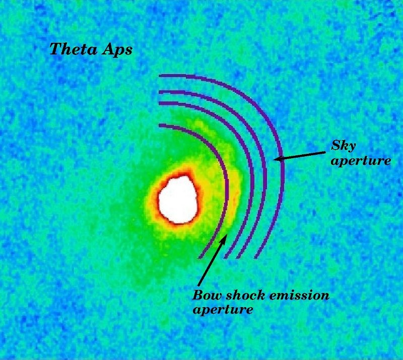
Figure 5: Illustration of the extended flux measurements of the observed bow shock of $\theta$ Aps. Both the elliptical bow shock aperture and the sky aperture are indicated.

3.2 Radial distance of arcs and detached shells

For some objects the extended emission is very faint with a low contrast with respect to the sky background. In order to improve the measurement of the angular distance/size of arcs and shells we have constructed radial profiles for Class II and Class III objects. Table 5 gives the radii of the “eyes” (II) and “rings” (III) as identified in the azimuthally averaged radial profiles shown next to the image panels in Figs. 2 and 3 (adopted azimuth angles are given at the top of each radial profile panel; for the “rings” objects it is alway 360°. For the “eyes” the radii and radial profiles of both arcs are given. For a few cases with very faint extended emission, the assignment is ambiguous. V Pav possibly belongs to Class III instead of Class II as the dust emission faintly traces a full circle. RT Cap is tentatively assigned to Class III but its ring is not complete and rather consists of two distinct arcs. However, the arcs are concentric, which is not the case for true “eye” objects. For S Cep the ring is also not complete but resembles more a full circle with gaps. The detached shell around Y CVn is very faint and barely visible at a radius of $\sim$190″, but in this case the detection is supported by the radial profile and its earlier detection with ISO/ISOPHOT by Izumiura et al. (1996). Tentatively, a faint arc bow shock structure (“fermata”) extending over $\sim$100°  (from position angle $\sim$30° to 130°) is present at 9′ east of the central star. X TrA is also listed in Class III although also here the ring is faint, with only a brighter arc to the east. Further observations are necessary to resolve these ambiguities.

Table 5: Aperture flux of observed bow shocks (Class I and II) and detached rings (Class III). Irregular Class IV is excluded. An elliptical annulus was applied in order to measure flux in the non-spherical arcs. The annuli of the detached rings were nearly spherical. The shape of the elliptical annulus was identified from the image with the most significant detection and then directly applied to the other band. For the fermata the flux is only integrated over a limited azimuthal angle covering the observed emission.

IRAS id	Object	Class	Radius		Dust annulus	Flux (Jy)		$M_{\rm dust+gas}$ ($10^{-4}$ M⊙)		$M_{\rm ISM}$	$M_{\rm ISM}$
			(″)	(pc)	(″)	70 $\mu$m	160 $\mu$m	70 $\mu$m	160 $\mu$m	($10^{-4}$ M⊙)	($10^{-4}$ M⊙)
00248+3518	AQ And	I+III	52	0.21	40-62 (circle)	2.20$\pm$0.01	1.28$\pm$0.01	0.9	1.1	1.1	4.4
01159+7220	S Cas	III	50	0.23	32-64	2.26$\pm$0.01	1.11$\pm$0.02	1.1	1.1	12	54
01246-3248	R Scl	I	54	0.10	51-68 (arc)	1.27$\pm$0.01	0.49$\pm$0.01	0.2	0.2	0.1	0.3
		III	14	0.03
02168-0312	$o$ Cet	I	82	0.04	70-150 (arc)	47.64$\pm$0.03	9.75$\pm$0.05	2.2	1.0	0.5	0.2
03374+6229	U Cam	III	7	0.02
		II	57/62	0.12/0.13	80-140	2.87$\pm$0.02	2.44$\pm$0.05	0.6	1.1	40	1110
03507+1115	NML Tau	I	85	0.10	95-130 (arc)	5.23$\pm$0.02	3.04$\pm$0.03	0.6	0.8	3.5	62
04459+6804	ST Cam	II	67/84	0.14/0.17	84-122	1.28$\pm$0.02	0.61$\pm$0.03	0.3	0.3	3.1	2.2
05028+0106	W Ori	I/III	92	0.17	70-120	1.99$\pm$0.02	0.62$\pm$0.03	0.4	0.3	8.2	32
05418-4628	W Pic	I	34	0.08	62-90	0.92$\pm$0.01	0.25$\pm$0.02	0.2	0.1	2.7	13
05524+0723	$\alpha$ Ori	I	397	0.25	510-660 (arc)	56.68$\pm$0.19	22.64$\pm$0.38	3.8	3.2	201	490
06331+3829	UU Aur	I	82	0.14	100-140 (arc)	5.44$\pm$0.02	2.50$\pm$0.03	0.9	0.9	14	88
09448+1139	R Leo	I	93	0.03	94-134	9.44$\pm$0.02	2.91$\pm$0.03	0.2	0.1	0.1	2.1
09452+1330	CW Leo	I	507	0.29	560-710 (arc)	6.88$\pm$0.08	10.13$\pm$0.11	0.4	1.4	76	31
		I					6.00$\pm$0.13		0.8
10329-3918	U Ant	III	42	0.06	30-55 (circle)	16.32$\pm$0.01	4.68$\pm$0.01	2.2	1.3	0.4	5.3
10350-1307	U Hya	I+III	114	0.12	100-133 (circle)	17.44$\pm$0.03	9.33$\pm$0.03	1.8	2.1	1.7	0.03
10416+6740	VY UMa	II	38/46	0.07/0.09	38-88	3.60$\pm$0.01	2.33$\pm$0.02	0.7	1.0	0.7	2.5
10580-1803	R Crt	II	$\sim$140	0.18	165-270	5.07$\pm$0.07	6.42$\pm$0.11	0.7	1.8	21	58
12427+4542	Y CVn	III	$\sim$190	0.30	150-260	5.14$\pm$0.07	3.79$\pm$0.10	0.8	1.3	7.7	2.9
13001+0527	RT Vir	I			50-140 (circle)	5.15$\pm$0.03	3.30$\pm$0.04	0.4	0.5	0.6
13269-2301	R Hya	I	96	0.05	200-245 (arc)	4.65$\pm$0.02	1.93$\pm$0.03	0.3	0.3	3.8	12
13462-2807	W Hya	III	68,230	0.03, 0.12	70-108 (ellipse)	21.28$\pm$0.02	6.08$\pm$0.03	1.1	0.7	0.2	0.1
14003-7633	$\theta$ Aps	I	76	0.04	118-146 (arc)	2.15$\pm$0.01	0.76$\pm$0.02	0.1	0.1	1.3	0.4
15094-6953	X Tra	III	150	0.18	60-210	9.70$\pm$0.08	6.89$\pm$0.12	1.8	2.7	106	21
16011+4722	X Her	I	45	0.03	40-90 (ellipse)	9.17$\pm$0.01	3.23$\pm$0.02	0.6	0.5	0.2	0.2
17389-5742	V Pav	II	97/100	0.17/0.18	95-140	1.30$\pm$0.03	1.50$\pm$0.04	0.2	0.6	21	12
18476-0758	S Sct	III	70	0.13	30-90 (circle)	14.09$\pm$0.02	8.85$\pm$0.03	2.7	3.7	13
19126+3247	W Aql	II	45/75	0.07/0.12	36-86 (ellipse)	11.10$\pm$0.02	4.25$\pm$0.03	1.9	1.6	5.8	144
19233+7627	UX Dra	II	76/54	0.14/0.10	50-110	2.89$\pm$0.01	1.11$\pm$0.03	0.6	0.5	4.4	2.5
19314-1629	AQ Sgr	I	57	0.09	50-100	3.44$\pm$0.02	2.53$\pm$0.02	0.6	0.9	5.4	3.7
19390+3229	TT Cyg	III	33	0.07	26-43 (circle)	1.74$\pm$0.01	0.86$\pm$0.01	0.4	0.4	1.3	21
20038-2722	V1943 Sgr	I	66	0.06	50-130 (arc)	5.98$\pm$0.03	2.30$\pm$0.03	0.6	0.5	2.6	0.8
20075-6005	X Pav	I	50	0.07	94-122	5.74$\pm$0.01	2.69$\pm$0.02	0.6	0.5	3.1	19
20141-2128	RT Cap	III	92	0.13	62-118	2.21$\pm$0.02	0.91$\pm$0.04	0.3	0.3	4.0	15
20248-2825	T Mic	I			40-100 (ellipse)	5.48$\pm$0.02	0.58$\pm$0.03	0.6	0.1	1.2
21358+7823	S Cep	III	90	0.18	70-130	2.14$\pm$0.03		0.4		11	142
21419+5832	$\mu$ Cep	I	78	0.15	100-150	28.64$\pm$0.04	11.5$\pm$0.12	5.6	4.8	56	637
21439-0226	EP Aqr	I	43	0.03	45-68	4.65$\pm$0.01	1.36$\pm$0.01	0.2	0.1	0.1	1.2
23438+0312	TX Psc	III	16	0.02
		I	38	0.05	12-58 (ellipse)	4.79$\pm$0.01	1.07$\pm$0.02	0.7	0.3	0.2	0.7
23558+5106	R Cas	I	97	0.06	100-160 (arc)	8.35$\pm$0.01	3.52$\pm$0.04	0.5	0.5	2.5	2.9

3.3 Far-infrared dust emission

Cold dust grains emit strongly at mid- to far-infrared wavelengths. Dust emission can, in a simple approximation, be described as a blackbody modified by the grain emissivity; $F_{\nu}\propto B_{\nu}\cdot Q_{\nu}$, with $Q_{\nu}\approx\nu^{\beta}$, where $\beta$ depends on the type of dust considered. For example, $\beta=1.1$ for amorphous carbon in the ISM (Rouleau & Martin 1991) as well as for carbon grains in carbon stars (Jura 1986), while astronomical silicates have $\beta=2$ (Volk & Kwok 1988).

Only for fast shocks ($v_{\rm shock}>50$ km s^-1) high shock temperatures are reached that give rise to UV radiation (e.g. observed for the bow shock of CW Leo) and possibly a strong [O i] 63 $\mu$m line. But, as the grains are only weakly coupled to the gas, due to the low densities, $T_{\rm dust}\ll T_{\rm gas}$. Low velocity shocks on the other hand give primarily rise to dust emission in the infrared. Despite observational efforts with Spitzer and Herschel, no infrared line emission has been detected in AGB star bow shocks yet (Ueta 2011; Decin et al. 2011), and we will assume here that the observed emission is entirely due to thermal dust emission (see also Sect. 4).

In Table 5 we give the aperture flux measured in both PACS bands for the elliptical bow shocks and circular rings. To determine the appropriate aperture we fit the extended dust emission with an ellipse. The inner and outer annulus of the aperture are subsequently derived from the azimuthally averaged radial profile. For detached rings the fitted ellipse is circular and the aperture is taken over the entire annulus. Bow shocks have a nearly elliptical shape, and their aperture flux is determined over a limited azimuthal angular range of the annulus. An illustrative example of a bow shock aperture measurement is shown for $\theta$ Aps in Fig. 5. Table 5 shows that the 70 over 160 $\mu$m flux density ($F_{\nu}$) ratio varies between 1.2 and 3.5, corresponding to a dust temperature of $\sim$30 to 40 K (for $\beta=2$).

The observed infrared flux – for optically thin emission – gives a direct measure of the emitting dust mass, and thus – given a gas-to-dust ratio – the total mass. Assuming specific dust properties one can write (Li 2005):

$$M_{\rm dust}=\frac{d^{2}F_{\lambda}}{\kappa(\lambda)B_{\lambda}(T)}=\frac{d^{2}F_{\nu}}{\kappa(\nu)B_{\nu}(T)}$$ (1)

with $F_{\nu}$ the observed flux (in erg s^-1 cm^-2 Hz^-1), $\lambda$ the wavelength (in cm), $d$ the distance (in cm), $T_{\mathrm{dust}}$ the dust temperature (in K), $B_{\nu}$ the Planck black body curve in frequency units, and and$\kappa_{\nu}$ the dust opacity at the observed wavelengths. We adopt a dust opacity of 60 and 10 cm² g^-1 at 70 and 160 $\mu$m, respectively (from Li & Draine 2001 who give $\kappa(\lambda)=2.9210^{5}(\lambda/\mu\mathrm{m})^{-2}$, i.e. $\beta=2$). For the dust temperature we adopt 35 K (as derived above), which means the dust is slightly heated with respect to the cirrus dust ($T_{\rm dust}\sim$15 to 20 K; Boulanger 2001). The estimated total dust and gas masses (adopting an average gas-to-dust ratio of 200) emitting in the bow shock region or detached shell are summarised in Table 5. The total observed masses range from $\sim 1\times 10^{-5}$ to $\sim 6\times 10^{-4}$ M_⊙. We note that the dust mass inferred from the measured infrared emission is sensitivy to the dust temperature, which is not well constraint by the avaialbe data, the dust emissivity law ($\kappa(\lambda)$), which is uncertain by order of magnitude and strongly dependent on the chemical composition of the dust, as well as the gas-to-dust ratio.

The total mass of the ambient medium that could be swept up by the stellar wind is roughly the volume set by the stand-off distance of the bow shock or the radius of the detached ring, $r$, times the mass volume density: $M_{\rm shell,ISM}=4/3\pi\ r^{3}\ \rho_{\rm ISM}$. In Table 5 we give $M_{\mathrm{ISM}}$ using both the ISM densities, $n_{H}$, derived using eq. 5 as well as using $n_{H}$ inferred from the measured stand-off distance and Eq. 2. For may cases the observed gas & dust mass is less than the potential swept-up ISM mass, but in a few cases the derived masses are similar. The potentially swept-up ISM mass, $M_{\mathrm{ISM}}$ ranges from 10^-5 to 10^-1 M_⊙. In comparison, assuming constant mass-loss rates, the stellar mass loss after 1000 years amounts too $1$ – $50\times 10^{-4}$ M_⊙, again similar to the observed total mass. This consistency is not surprising, since to first order, the total mass accumulated in the bow shock depends on its age (i.e. mass of stellar material piled-up) and the ISM density (mass of swept-up ambient ISM material). However, for bow shocks (spanning a limited azimuthal angle), only a fraction – typically less than half – of the stellar wind and ISM material is entrained into the bow shock region. Furthermore, both ISM and wind material flow from the bow shock apex along the contact discontinuity to be finally shed in the tails. For detached shells, both the ISM and stellar wind mass are presumably preserved, unless either formation or destruction of dust grains and molecules alters the gas-to-dust ratio and its chemical composition (e.g.  photo-destruction of CO by the ISRF or processing of grains in the shock).

4 Interaction between stellar winds and the ISM

Bow shocks are common in astrophysical contexts and can occur where two material flows – of different density, velocity, or viscosity – collide. Examples are bow shocks around compact H ii regions due to stellar winds (van Buren et al. 1990, Mac Low et al. 1991; Raga et al. 1995), but also due to winds in binary systems (Stevens et al. 1992; Parkin & Pittard 2008; Pittard 2009; van Marle et al. 2011a), or movement of an object with a magnetic field through a medium (Baranov et al. 1971, Cordes et al. 1993), between slow and fast winds (Steffen et al. 1998; Steffen & Schönberner 2000), and between stellar winds and the surrounding ISM (Matsuda et al. 1989; Brighenti & D’Ercole 1995; Comeron & Kaper 1998).

In this section we will discuss the formation of bow shocks due to interaction of a stellar wind with a low density medium. First the general case of a star with a stellar wind moving through the ISM is considered. We discuss also the special case of a stationary star with a stellar wind expanding into either an older stellar wind or the interstellar medium.

4.1 The size and shape of a bow shock due to “wind-ISM” interaction

If a supersonic stellar wind and the ambient medium collide, a bow shock interface can be created at a distance from the moving star where the ram pressures and momentum fluxes of the wind and the ISM balance each other. This is called the contact discontinuity. It is a result of interaction between two fluids, but shocks are not necessary. In the absence of shocks, there will be only collisional heating and no H$\alpha$ emission. For shocks to occur the Mach number $M$ of the fluid velocity $v$ ($M=v/v_{\rm sound}$) should be higher than unity. I.e. the relative velocity between the stellar wind and ISM needs to be higher than the speed of sound in the ISM. Note however that the speed of sound in the low density isothermal warm neutral medium (WNM) is very low ($v_{\rm sound}\sim 1$ km s^-1) and thus even a slow AGB wind ($v_{w}\sim 10$ km s^-1) will move supersonically. Because the sound speed (adiabatic case; $\gamma=5/3$) scales with $(P/\rho)^{1/2}$ (or T^1/2)) the sound speed will be lower in the diffuse cold neutral medium (CNM). In the non-adiabatic regime the ram pressure balance is given by $\rho_{w}v_{w}^{2}=\rho_{\rm ISM}v_{\rm ISM}^{2}$. Assuming that the layers mix and that the post-shock cooling is efficient (i.e. instantaneous cooling), the thickness of the dense shell is negligible with respect to the distance from the star. This is, for example, valid for a slow stellar wind interacting with a hot low-density medium (Borkowski et al. 1992). In this approximation the stand-off distance, $R_{0}$, defined as the distance between the star and the apex of the contact discontinuity or bow shock, is given by (e.g. Baranov et al. 1971; Dyson 1975; Raga et al. 1995, Wilkin 1996):

$$R_{0}=\sqrt{\frac{\dot{M}\ v_{w}}{4\pi\ \rho_{\rm ISM}\ v^{2}_{\star}}}$$ (2)

with $\dot{M}$ the rate of mass loss and $v_{w}$ the velocity of the isotropic stellar wind (with respect to the rest-frame of the star), $\rho_{\rm ISM}$ the mass density of the ambient ISM, $v_{\star}$ the relative space velocity of the star with respect to the ISM. The standard bow shock morphology consists of a forward shock separating the unshocked and shocked ISM, a wind termination shock that separates the free-streaming wind from the shocked wind, and between them a contact discontinuity separating the shocked wind from the shocked ISM (see e.g. Weaver et al. 1977 and Lamers & Cassinelli 1999). If the cooling of the shocked stellar wind is inefficient, a thick hot, low-density gas layer will exist between the free-flowing wind and the bow shock. The termination (reverse) shock and the bow shock, delineating the contact discontinuity, both travel away from this contact discontinuity; the bow shock in forward direction and the termination shock in backward direction with respect to the relative motion of the star in a stationary ISM.

As mentioned above, for efficient cooling, the physical thickness of the shocked region remains small and thus the two shock fronts delineating the contact discontinuity are not resolved. In Sect. 6 we present hydrodynamical simulations of wind-ISM interaction which explore the effect of varying the parameters used in Eq. 2 ($\dot{M}$, $v_{\star}$, $n_{\mathrm{H}}$) as well as other parameters such as the dust-to-gas ratio and the temperature of the ISM. These simulations also confirm that, despite the formation of turbulent instabilities and inefficient cooling in some cases, Eq. 2 gives in general a rather accurate prediction for the stand-off distance.

Adopting appropriate values for the mass-loss rate, stellar wind velocity, the star’s velocity, and the ISM density (Sect. 5), we can directly predict the stand-off distance, $R_{0}$ from Eq. 2. This predicted value for $R_{0}$ can then be compared directly to the measured $R_{0}$ obtained by de-projecting the observed minimum distance between the star and the bow shock outline. Vice versa, we can use the measured $R_{0}$ and Eq. 2 to derive $n_{\rm ISM}$. This is important as the local ISM density is difficult to determine observationally (see Sect. 5).

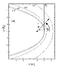
Figure 6: Observable projected outlines of wilkinoids for an $R_{0}$ of 1 and star-ISM motion inclinations of $i=0,25,50,$ and $75\degr$ (with respect to the line of sight). The stellar position is indicated by a star. $A$ is the observed (projected) stand-off distance between the star and the bow shock apex. $B$ is the observed (projected) distance between the star and the bow shock for $\theta=90$ °. $\theta$ for any point $x$ on the projected outline is the angle between the star-apex line and the line connecting the star with the point $x$.

For example, let us apply this to $\alpha$ Ori. The star is at a distance, $d=197$ pc ($z$ = -14 pc), moving at an intermediate velocity of 28.3 km s^-1 through the ISM (Ueta et al. 2008; van Marle et al. 2011b). Its mass-loss rate is $3\times 10^{-6}$ M_⊙ yr^-1 and the stellar wind velocity, $v_{w}=14.5$ km s^-1 (Table LABEL:tb:properties1). From the observed de-projected stand-off distance, $R_{0}$ of 5.0′ or 0.3 pc, the local ISM density is then found to be 4.2 cm^-3. This estimate is a factor of two higher than the density derived from the models of the ISM (Eq. 5, $n_{H}=1.7$ cm^-3). The predicted stand-off distance is close to that obtained from a detailed simulation of $\alpha$ Ori (see e.g. van Marle et al. 2011b and simulation A in Sect. 6).

The 2D-shape of the contact discontinuity (and thus also the termination shock and bow shock) can be solved analytically in the optically thin approximation (Mac Low et al. 1991; Raga et al. 1995, Wilkin 1996):

$$R(\theta)=R_{0}\frac{\sqrt{3(1-\theta\cot\theta)}}{\sin\theta}$$ (3)

with $\theta$ the latitudinal angle from the apex of the bow shock as seen from the position of the central star, and $R_{0}$, the stand-off distance defined in Eq. 2. Alternatively, it can be written as $y(z)=\sqrt{3}R_{0}\sqrt{1-z/R_{0}}$ (e.g. Mac Low et al. 1991; Fig. 6). Eq. 3 is valid only for the case of a relative star-ISM motion in the plane of the sky (i.e. a “side view” of the bow shock or a star-ISM motion inclination of $i=0$° with respect to the plane of the sky). In this case, $R_{0}$ is directly the angular separation, $A$, of the star to the observed bow shock outline (Fig. 6). Similarly, when there is no inclination($i$ = 0°), the angular distance between the star and the surface of the bow shock parabola at an angle of $\theta$ = 90°  (perpendicular to the apex direction from the star) can be defined as $B$, where $B=R(90\degr)=y(0)=R_{0}\sqrt{3}$ (Wilkin 1996 and Fig. 6). In this geometry, $R_{0}$ can also be derived from measuring the angular distance between the star and the bow shock interface at an angle of $\theta$ = 90° with respect to the star-ISM motion direction ($B$; as illustrated in Fig. 6), since $R$(90°) = y(0) = $R_{0}\sqrt{3}$ (Wilkin 1996).

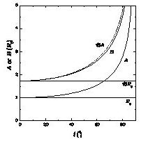
Figure 7: Observable bow shock properties $A$ and $B$ as a function of inclination $i$ for a fixed $R_{0}=1$.

In general the relative star-ISM motion will be inclined with respect to the plane of the sky, thus $i\neq 0$. In order to quantify the effects of an inclined bow shock with respect to the plane of the sky, we simulated the appearance of the three dimensional bow shock surface. This hollow paraboloid wilkinoid surface is defined by rotating the two dimensional shape, i.e. the R($\theta$) curve, around its axis of symmetry (which is defined by the line connecting the star and the bow shock apex). We numerically construct a 3D wilkinoid surface. These points are then projected onto the plane of the sky under a given inclination angle to compute the observable outline of the bow shock in the optically thin approximation. This outline thus traces the loci of tangential line of sight to the bow shock paraboloid at a given inclination angle. Four such constructed wilkinoids with an $R_{0}$ of 1 and star-ISM motion inclinations with respect to the plane of the sky of $i=0,25,50$, and $70$° are shown in Fig. 6 to illustrate the change in shape with increasing inclination angle. These simulations show indeed that for an increasingly higher inclination $i$ (corresponding to a smaller viewing angle with respect to the line-of-sight), the projected size of the bow shock outline becomes increasingly larger, which is qualitatively consistent with earlier bow shock simulations for compact H ii regions (Mac Low et al. 1991). As noted above, in Fig. 6 we also indicate the two observable quantities, $A$ and $B$. $A$ is the projected – minimal – distance between the star and the bow shock outline in the direction of relative motion, which can be measured directly from the observed image. $B$ is the distance perpendicular to $A$, i.e. at $\theta=90$°, from the star to the bow shock outline. It is important to note here that due to the inclination of the bow shock surface with respect to the line-of-sight, a “pseudo” apex of the observable outline appears where the line-of-sight becomes tangent to the rotated 3D-Wilkin paraboloid. The observable $A$ is in fact the distance from the star to this “pseudo”-apex projected onto the plane of the sky (i.e. not to the real apex of the wilkinoid). At high inclination, but less than 90°, both the “pseudo”-apex and true apex of the observable outline would appear – in the model – as two brightness enhancements. We refer the reader to Figs. 5 and 11 in Mac Low et al. (1991) for an excellent illustration of this effect. However, due to superposition of the true apex and the very bright central star the latter will not be detectable for our stars. In addition, the faint “pseudo”-apex will also be difficult to observe. For $i=90$° there is no tangent to the paraboloid, thus only the bow shock apex would theoretically appear as a spherical central peak brightness distribution, where it not for the fact that it will not be visible due to superposition with the very infrared bright central star. For the $i=0$°  (side view) the simulation gives indeed $A=R_{0}$ (i.e. the projected and de-projected stand-off distance are the same) and $B=R_{0}\sqrt{3}$ (also here the true apex is observed).

In Fig. 7 the $A$ and $B$ values, in units of $R_{0}$, are given as a function of the inclination $i$. Measuring both $A$ and $B$ would then, in principle, directly constrain both $R_{0}$ and $i$. Unfortunately, measuring both quantities in the detected bow shocks is often not possible due to irregularities and incompleteness of the bow shock. Also the change of outline with varying $i$ is a small effect, thus making the exact inclination angle and stand-off distance highly degenerate. For inclination angles $i<45$ ° the change in $A$ or $B$ is less than 10% (Fig. 7 and Mac Low et al. 1991). Only at large inclinations (or small viewing angles) does the observed projected distance $A$ to the bow shock outline differ significantly from $R_{0}$, the de-projected stand-off distance. Consequently, using these relations and the kinematical properties of the measured stars and its local ISM, inclination-corrected $R_{0}$ values can be derived by measuring $A$ and/or $B$ together with a calculated or assumed $i$. Thus, first a plausible inclination is derived from the space motion, secondly $A$ is measured from the observed image and thirdly, $R_{0}$ is obtained from the $R_{0}$-$A$ relation in Fig. 7. Ideally the star’s kinematical properties (proper motion and radial motion) would give the heliocentric 3D space motion vector of the star, wile the observed bow structure would – independently – yield the heliocentric 3D orientation of the bow, whose apex’s 3D orientation represents the heliocentric relative space motion of the star, with respect to the ISM. Thus, the difference of the two would yield the heliocentric 3D ISM flow vector. However, in order to circumvent the high degeneracy between $i$ and $R_{0}$ we use the space motion vector inclination angle $i$ to constrain $R_{0}$ from the observed bow shock shape, which thus neglects a potential ISM flow (see Sect. 5.1 for a discussion on the local LSR ISM velocity). Table LABEL:tb:properties1 gives the de-projected $R_{0}$ obtained via wilkinoid fitting as discussed above for the objects which show emission in the shape of an arc or shell, and thus potentially trace the dust emission outline of a bow shock.

4.2 Special cases of “wind-ISM” and “wind-wind” interaction

In the case of a (nearly) stationary star (with respect to the local ISM and compared to the stellar wind velocity), spherical symmetry of the stellar wind-ISM interaction is preserved (e.g. Libert et al. 2007). Nevertheless, there is a relative velocity difference between the stellar wind and the ambient medium. The interaction of a spherical outflow with external matter leads to the formation of a region of compressed material within two spherical boundaries (Weaver et al. 1977). As before, this region consists of a termination shock (where the freely expanding (supersonic) stellar outflow is abruptly slowed down by compressed material), a contact discontinuity (separating the circumstellar and interstellar matter) and the bow shock (external boundary at which the external medium is compressed by the expanding shell). It is thus a special case of a “wind-ISM” interaction scenario described in the previous section. The total mass of the detached shell would consist of both circumstellar and interstellar matter. The latter can be estimated from the total hydrogen mass that would have been present in a sphere of radius equal to the radius of the detached ring (Sect. 3.3).

However, the fact that the “external” material of the stellar wind is interacting with is moving together with the source (thus keeping the spherical symmetry) may also suggest that in fact the “external” matter is not genuine ISM but rather material remaining from an older mass-loss event, perhaps during the RGB phase. The thermal pulse scenario leads to an interaction between a slow and a fast wind, i.e. “wind-wind” interaction. In this case, $v_{\star}$ from Eq. 2 is the relative velocity between the slow and fast wind. In the rest frame of the star, the second wind is computationally equal to a flowing ISM. A detached dust shell is believed to result from an intense – relatively short – episode of enhanced mass-loss rate and wind velocity (e.g. initiated by a He-shell flash), whose wind has a higher outflow velocity and will thus interact with the previous slower wind. The subsequent sharp drop in mass-loss rate and outflow velocity for a few thousand years directly following the thermal pulse or He-flash will lead to a detached dust shell (e.g. Olofsson et al. 1990; Vassiliadis & Wood 1993; Steffen & Schönberner 2000; Mattsson et al. 2007). The (relative) jump in velocity and mass-loss rate from pre-flash to flash-peak is possibly the most critical parameter governing the formation of a detached shell (Mattsson et al. 2007). The latter scenario seems more appropriate for the formation of geometrically thin detached molecular shells with high expansion velocities showing little interaction with the surrounding medium. Indeed, the detection of bow shocks together with a small detached ring gives further support to this hypothesis. Another possibility could be that the ring represents the (inner) termination shock associated to the bow shock located further outwards. Other scenarios, such as constant mass-loss in combination with non-isotropic mass-loss events and clumpy dust formation have also been detected in the form of non-concentric spherical shells (Decin et al. 2011).

5 Stellar, circumstellar and interstellar properties

The relation (Eq. 2) between the stand-off distance of the bow shock region and the star’s mass-loss rate, $\dot{M}$, terminal wind velocity, $v_{w}$, peculiar velocity ($v_{\star}$), and the ISM density ($n_{\mathrm{H}}$) is powerful in its simplicity. For observed bow shocks around stars with known (observed) mass-loss properties and space motion, the local ISM density – which is often the most difficult to determine accurately – can be inferred directly from the measured stand-off distance. On the other hand, for stars with known stellar mass-loss, known space motions and (assumed) ISM densities, the stand-off distance can be predicted. In this section we review the relevant and available stellar properties of the observed AGB stars and supergiants as well as the properties of the local ISM. The interplay between these various physical properties determines the final shapes and sizes of the wind-ISM interaction zone, in particular the contact discontinuity as discussed in the Sect. 4.1. Adopting the stellar, circumstellar and interstellar properties presented in this section for each object in our survey, both the predicted ISM densities for observed bow shocks as well as predicted stand-off distances for all targets in the survey are given in Tables LABEL:tb:properties1 to LABEL:tb:properties2.

5.1 Stellar distance and (relative) space velocity

The parallax, proper motion, and the radial local standard of rest (LSR) velocities give a direct estimate of the distance, $d$, and the absolute peculiar space velocities, $v_{\star}$ (as per Johnson & Soderblom 1987), for the majority of the AGB stars and red supergiants. The LSR velocities have been corrected for the solar motion $v_{\odot}$ [($U,V,W$) = (11.1, 12.24, 7.25) km s^-1] (Schönrich et al. 2010). Parallaxes from re-processed Hipparcos data (van Leeuwen 2007) were taken, when available, if the uncertainties are less than 20%. For several (distant) stars, the parallactic distances derived from Hipparcos data have large uncertainties or have not been obtained at all. For these targets distances can be derived, for example, from the (pulsation) period-luminosity($K$) relation, and observed apparent $K$ magnitudes. A generic Galactic $P$-$K$ relation valid for both oxygen- and carbon-rich (Mira) variables was established by e.g. Whitelock et al. (2000, 2008): $M_{K}=-3.51[{\log}\ P-2.38]-7.25$. Vlemmings et al. (2003) obtained VLBI parallaxes for four Miras that were more consistent with distances derived via the $P$-$K$ relation than those obtained with Hipparcos. Tables LABEL:tb:properties1 to LABEL:tb:properties2 give the derived peculiar velocities and peculiar absolute proper motions with their associated position angles.

Radial (LSR) velocities are taken from CO line surveys where available. Primary sources are De Beck et al. (2010) and Menzies et al. (2006), which have good agreement for sources in common to both studies (typically the differences are less than 3 km s^-1).

At this point we assume that the relative peculiar velocity between the ISM and the star, $v_{\star}$, is determined entirely by the star space velocity with respect to the local standard of rest (LSR) (i.e. the stationary ISM). In other words, we assume that there is no flow of the ISM itself. This could be a simplification for some cases where the ISM may have an appreciable flow velocity as matter is being blown away by super-bubbles (see Ueta et al. 2009a, b for the case of $\alpha$ Ori).

To test this, we estimate the local LSR ISM velocity ($v_{r},v_{l},v_{b}$) from the galactic rotation (Oort 1928, Feast & Whitelock 1997) at the position of the stars and correct $v_{\star}$ to obtain the local $v_{\star-\rm ISM}$. For the majority of the objects the $v_{\star-\rm ISM}$ is within $\pm$20% of $v_{\star}$, thus decreasing/increasing the predicted stand-off distance by the same factor. Only in a few cases this correction gives a significant change in peculiar velocity; for U Cam, V Hya, T Lyr, and $\mu$ Cep this gives relative space velocities that are approximately a factor of 1.5 higher, and for Y Pav a factor of 2 lower.

The average space velocity, $v_{\star}$, for our sample of stars is $\sim$36 km s^-1  (Tables LABEL:tb:properties1 to LABEL:tb:properties2), consistent with the average velocity of $\sim$30 km s^-1 for Galactic AGB stars (Feast & Whitelock 2000).

5.2 Mass-loss rate

The mass-loss rate of evolved stars is important for the enrichment of the ISM. It also directly affects the shape and size of the stellar wind-ISM interaction (Sects. 4 and 6). Mass-loss rates can be estimated directly via modeling of observed CO line profiles (e.g. Knapp et al. 1998; Groenewegen & de Jong 1998; Groenewegen et al. 2002; De Beck et al. 2010). In general the derived (gas) mass-loss rates depend on the line strength, terminal gas expansion velocity ($v_{w}^{2}$), and distance ($d^{2}$). The average gas mass-loss rate from $\sim$300 Galactic carbon stars is $1.1\times 10^{-5}$ M_⊙ yr^-1 (Groenewegen et al. 2002). The latter should probably be reduced by an order of magnitude since new Hipparcos results show that the distances adopted by Groenewegen et al. (2002) are over-estimated by a factor of two to four. Using CO-derived mass-loss rates, an empirical relation has been established between the mass-loss rate and luminosity variability period (e.g. De Beck et al. 2010): log($\dot{M}$) = -7.37 + 3.42 $\times$ 10^-3 P (for P $\leq$ 800 days) and log(Ṁ) = -4.46 (for P $\geq$ 850 days), with $\dot{M}$ in units of M_⊙ yr^-1. However, the scatter on this relation is rather large with a typical uncertainty of a factor of 10 (see De Beck et al. 2010 for details). Similar results are obtained for carbon Mira variables by Groenewegen & de Jong (1998): log($\dot{M}$) = 4.08 log $P$ - 16.54. Adopted mass-loss rates – based on CO observations or luminosity period – are included in Tables LABEL:tb:properties1 to LABEL:tb:properties2. If neither $\dot{M}$ nor period are available, we adopt a generic value of $5\times 10^{-7}$ M_⊙ yr^-1. Uncertainties in $\dot{M}$ arise predominantly from inaccurate distance determinations for distant stars.

5.3 Stellar wind velocities

For the (terminal) wind velocity, $v_{w}$, we adopt the terminal velocity of the CO envelope (e.g. De Beck et al. 2010; Tables LABEL:tb:properties1 to LABEL:tb:properties2 and references therein). Groenewegen et al. (2002) find an average expansion velocity of 18.7$\pm$6.1 km s^-1 for a sample of 330 carbon stars. For a set of 24 oxygen-rich and 13 carbon-rich AGB stars, De Beck et al. (2010) find mean $v_{w}$ values of 14.5 and 15.4 km s^-1, respectively. These values are 4-10 km s^-1 higher than those of Ramstedt et al. (2006) for a set of 77 oxygen-rich and 61 carbon-rich stars. For carbon-rich stars, this average is $\sim$3 km s^-1 lower than the one found by Groenewegen et al. (2002). If no CO terminal velocities are available, we adopt a generic value of $v_{w}=15$ km s^-1, for both oxygen- and carbon-rich stars.

5.4 Local interstellar medium density

The ambient (uniform) mass density of the ISM is defined as $\rho_{\rm ISM}=\mu_{\mathrm{H}}\ m_{\mathrm{H}}\ n_{\mathrm{H}}$, with $\mu_{\mathrm{H}}=1.4$, the mean nucleus number per hydrogen atom for the local medium, $m_{H}$ is the mass of the hydrogen nucleus, and $n_{\mathrm{H}}$ the interstellar hydrogen nucleus density. Although the ISM is far from uniform, there is a general dependence between the interstellar matter (space-averaged) volume density, $n_{\rm ISM}$, and $z$, the distance from the Galactic plane.

The different phases of the ISM have different average densities, scale-heights and filling factors (see e.g. Savage 1995; Boulanger 2001; Ferrière 2001; Wooden et al. 2004; Cox 2005). Dickey & Lockman (1990) used radio observations of H i to derive the structure of the CNM, WNM and WIM (warm ionised medium):.

$$n_{H}(z)=0.39\ e^{-\left(\frac{z}{127\rm pc}\right)^{2}}\ +\ 0.11\ e^{-\left(\frac{z}{318\rm pc}\right)^{2}}\ +\ 0.06\ e^{-\frac{|z|}{403\rm pc}}$$ (4)

Based on UV observations of H i and H₂, Savage et al. (1977) and Diplas & Savage (1994) arrive at a similar result for the WNM as Dickey & Lockman (1990). An alternative relation is given by Loup et al. (1993) which is based on Spitzer (1978) (density $n_{\mathrm{H}}$(z=0) = 2 cm^-3) and Mihalas & Binney (1981) (scale height of 100 pc):

$$n_{H}(z)=2.0\ e^{-\frac{|z|}{100\rm pc}}$$ (5)

These two relations are shown further below in Fig. 11 (Sect. 7). Thus, we obtain some first insights into the local ISM density for our objects (Tables LABEL:tb:properties1 to LABEL:tb:properties2). Evidently, one should be cautious using these relations for specific cases as there is structure in the ISM on all spatial scales, with different phases that have different filling factors. For example, diffuse to molecular clouds ($n_{H}\sim 10-1000$ cm^-3) have an order of magnitude lower filling factor than the low density WNM and WIM surrounding it. Thus, statistically about 10% of the objects in our survey could be moving through a denser medium than inferred from the above relation for the WNM. Generally, these relations do indicate that $n_{\mathrm{H}}$ drops as one moves away from the Galactic plane, leading to – on average – lower volume densities of the ISM. We use Eq. 5 to get a first estimate of the local ISM density for the objects in this survey (Tables LABEL:tb:properties1 to LABEL:tb:properties2). Accurate measurements of the local ISM density for all stars in our sample would be desirable, but are currently – to the best of our knowledge – unavailable. In fact, we will show that for certain cases the observations of bow shocks can potentially be used, via the measurements of the stand-off distances, to derive estimates of the local ISM density.

5.5 Circumstellar chemistry, spectral type and binarity

In addition to the above stellar properties that have a direct impact on the theoretical stand-off distance via Eq. 2, other possibly pertinent information such as spectral types of the central star and dominant circumstellar chemistry (oxygen versus carbon rich), and binarity is also included in Tables LABEL:tb:properties1 to LABEL:tb:properties2. If and how these stellar attributes could affect the occurrence and shaping of bow shocks is discussed further in Sect. 7.

Table 6: Parameters for the moving star simulations.

label	description	$\dot{M}$	$M_{\rm dust}/M_{\rm gas}$	$v_{\star}$	$n_{\rm ISM}$	$T_{\rm ISM}$	physical space	basic grid	$R_{0}$	$R_{s}$
		($\mathrm{M}_{\odot}$ yr-1)	(%)	(km s-1)	(cm-3)	(K)	(pc)		(pc)	(pc)
A	basic model	$10^{-6}$	1	25	2	1	1.5x1	$120\times 80$	0.26 $\pm$ 0.01	0.35
B	high $\dot{M}$	$10^{-5}$	1	25	2	1	2x2	$160\times 160$	0.59 $\pm$ 0.03	0.73
C	low $\dot{M}$	$10^{-7}$	1	25	2	1	2x1	$160\times 80$	0.090 $\pm$ 0.001	0.10
D	low dust	$10^{-6}$	0.1	25	2	1	2x1	$160\times 80$	0.33 $\pm$ 0.03	0.33
E	high $v_{\star}$	$10^{-6}$	1	75	2	1	1.5x1	$120\times 80$	0.11 $\pm$ 0.02	0.13
F	low $n_{\rm ISM}$	$10^{-6}$	1	25	0.2	1	3x2	$240\times 160$	0.76 $\pm$ 0.08	0.92
G	warm ISM	$10^{-6}$	1	25	2	8 000	2x2	$160\times 80$	0.31 $\pm$ 0.06	0.45

6 Hydrodynamical models of interaction between the slow stellar wind of a moving star and the ISM

Hydrodynamical simulations offer the opportunity to explore the effect of varying physical properties of either the stars (e.g. mass-loss rate, wind and (relative) space velocity) and/or the ISM (density, temperature) in a coherent systematic way. For example, Steffen & Schönberner (2000) and Libert et al. (2007) used hydrodynamical simulations to show that a brief episode of increased mass-loss rate could give rise to an expanding, geometrically thin shell. Wareing et al. (2006b) applied numerical simulations of a two-wind model to explain the observed structure around R Hya. Simulations by Wareing et al. (2007a) and Wareing et al. (2007b) indicate that a higher mass-loss rate (for similar ISM density and space velocity) will result in more pronounced Kelvin-Helmholtz instabilities (see their Fig. 1). Wareing et al. (2006a) obtain bullet-shaped emission structures simulating a PN (their Figs. 3 and 5). Villaver et al. (2003) include time-dependent mass-loss in simulations of wind-ISM interaction, leading to time-dependent stand-off distances.

One particular strength of hydrodynamical simulations is that they allow to study the formation, growth and dissipation of fluid instabilities – like Rayleigh-Taylor (RT) and Kelvin-Helmholtz (KH) instabilities – important in wind-ISM shock interactions. RT instabilities occur when a dense, heavy fluid is accelerated by a light fluid. Normally two plane-parallel fluid layers are meta-stable, but a small perturbation can destroy this delicate equilibrium. This manifests itself as so-called inter-penetrating “RT-fingers”. Such instabilities could be quenched by a restoring force such as a magnetic field, thus preventing these instabilities to grow (Chandrasekhar 1961). The KH instability results from a velocity shear between two fluid layers. This flow of one fluid over another will induce a centrifugal force which leads to changes in pressure which amplifies the ripple. Together with a RT instability, the KH instability will form structures in the shape of mushroom caps on the end of the RT fingers. The KH time-dependent turbulent eddies can form a complex structure arising in a steady flow, if they become large enough to influence that large-scale morphology of the shocked gas. Other instabilities that can occur are the non-linear thin shell instability (Vishniac 1994) and the transverse acceleration instability (Dgani et al. 1996) as shown numerically by e.g. Blondin & Koerwer (1998) and Comeron & Kaper (1998).

6.1 Hydrodynamical simulations

Here we present a series of seven simulations of the interaction between the ISM and the circumstellar medium of moving, evolved stars in order to find out how the morphology of the bow shock varies with the various stellar wind and ISM parameters. The different pertinent parameters for the simulations are summarised in Table 6. For our hydrodynamical simulations we use the MPI-AMRVAC code (Keppens et al. 2011). This code solves the conservation equations of hydrodynamics on an adaptive mesh (AMR) grid. We use a 2-D cylindrical grid in the r-z plane. The basic resolution is set at 80 grid points per parsec, but allows four additional levels of refinement, each doubling the effective resolution. This gives us a maximum effective resolution of 1280 grid points per parsec. Since some of the models require a larger physical space we use grids of different sizes for those simulations. In those cases we increase the number of grid points on the basic level to maintain the same resolution. The expanding stellar wind is inserted by filling a small circle with wind material. The motion of the star is handled by giving the ambient medium around the star a velocity in the z-direction. Therefore, we are simulating the wind interaction in the frame-of-reference of the star. Since all models are 2-D and the simulated space lies along the direction of motion of the star, the snapshots (Figs. 8 through 10) show projections for $i=0$.

To the basic conservation equations we have added the effect of optically thin radiative cooling. This is necessary since some of the shocks are strongly radiative, which changes the morphology of the shocked gas. In the case of simulation G, where the ISM has a high temperature, we put a lower limit on the cooling in the ISM, so that in the ISM the temperature does not fall below 8 000 K. More importantly, we have also added a (simplified) dust component (van Marle et al. 2011b). This is done by using a two-fluid approximation, with the dust represented as a gas without internal pressure. For simplicity we only include dust in the wind and neglect the dust component of the ISM. This gives us a set of five partial differential equations (not counting the vector components) for the pressure balance for the gas and dust. For the gas we have conservation of mass, momentum and energy, while for the dust we only have conservation of mass and momentum. The appropriate equations are given in van Marle et al. (2011b). Radiative losses depend on the hydrogen and electron particle densities (derived from $\rho$ assuming full ionization with hydrogen mass and involve a temperature dependent cooling curve $\Lambda(T)$. This cooling curve has been calculated with the CLOUDY code (Ferland et al. 1998) and includes radiative losses through IR radiation from the dust. We also include a drag force linking the gas and dust, which is derived from a combination of Epstein’s drag law for the subsonic regime and Stokes’ drag law for the supersonic regime (Kwok 1975, see also van Marle et al. 2011b). The drag force depends on the dust particle density and radius (0.005 $\mu$m), the velocity difference between gas and dust, as well as the thermal speed of the gas (Kwok 1975). For further details we refer the reader to van Marle et al. (2011b).

Since our equations are purely hydrodynamical, we don’t take into account magnetic fields or the effect of radiation on the dust particles. We also neglect destruction and creation of dust particles. Radiative processes are not included and thus the dust temperature cannot be treated appropriately (currently only collisional heating of dust could be accounted for). Also the gas is purely heated by collisions, and cooled radiatively; photo-ionisation is not included. Introducing radiative cooling by dust will cause the bow shock to become thinner and more unstable.

Adding destruction processes such as collisional heating or UV irradiation could, in principle, be included, but at a high cost in the required computing time. Both mechanisms are not expected to be very efficient as grains are not easily destroyed, because they are very effective radiators (emitting all heat immediately in the infrared) and the shocks discussed here are not very strong, and the radiation field would not be strong enough to destroy grains. Furthermore, dust can also be created in the high density shock regions, thus lowering the effective dust destruction rate. Further details are given in van Marle et al. (2011b).

The input and grid parameters are summarised in Table 6. We start with a basic model (simulation A), which has input parameters based on the observations of $\alpha$-Orionis (Ueta et al. 2008). Using this model as a starting point, we vary individual parameters to investigate the effect on the morphology of the bow shock. Note that for a stationary star, $v_{\star}=0$ km s^-1, the shock between the wind and ISM will drive a spherical shell of wind material sweeping up the ISM material, thus leading to detached shells / rings (not shown).

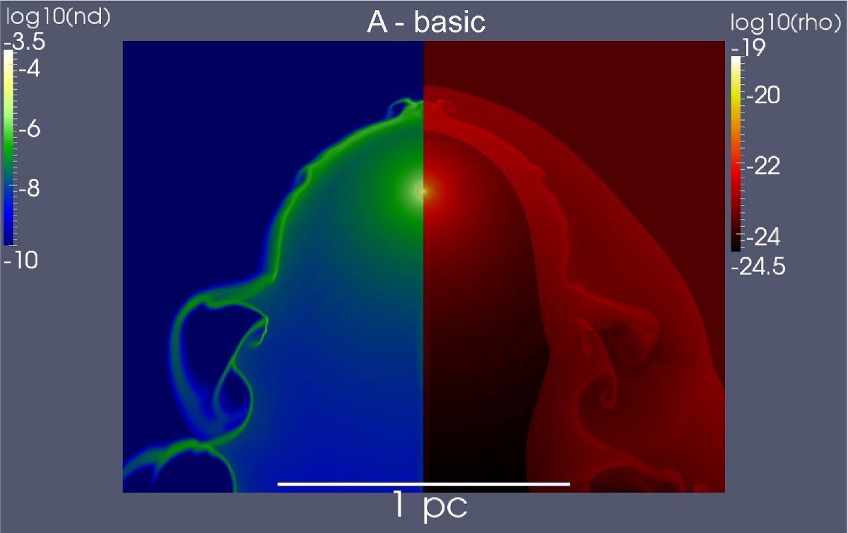
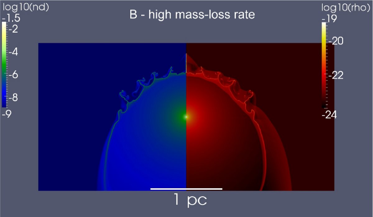
Figure 8: Top panel (A): Gas density in g/cm³ (right) and dust grain particle density in cm^-3 (left) for simulation A after 1.37$\times 10^{5}$ years; basic model. The bow shock is smooth, but at the contact discontinuity both Rayleigh-Taylor and Kelvin-Helmholtz instabilities are visible. Bottom panel (B): Similar to top panel, but for simulation B after 5.0$\times 10^{4}$ years; high $\dot{M}$. The instabilities are now primarily of the Rayleigh-Taylor type. Due to the stronger wind the bow shock lies further from the star.

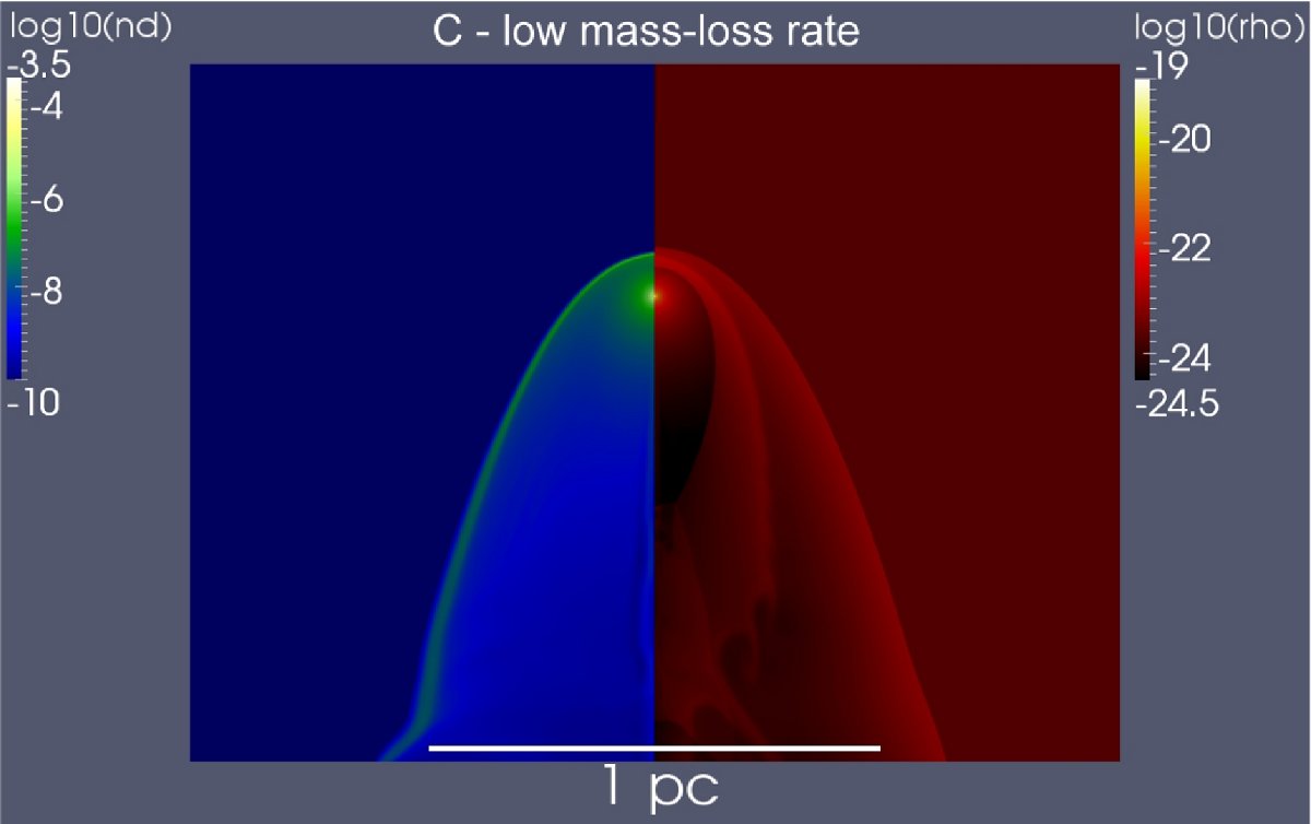
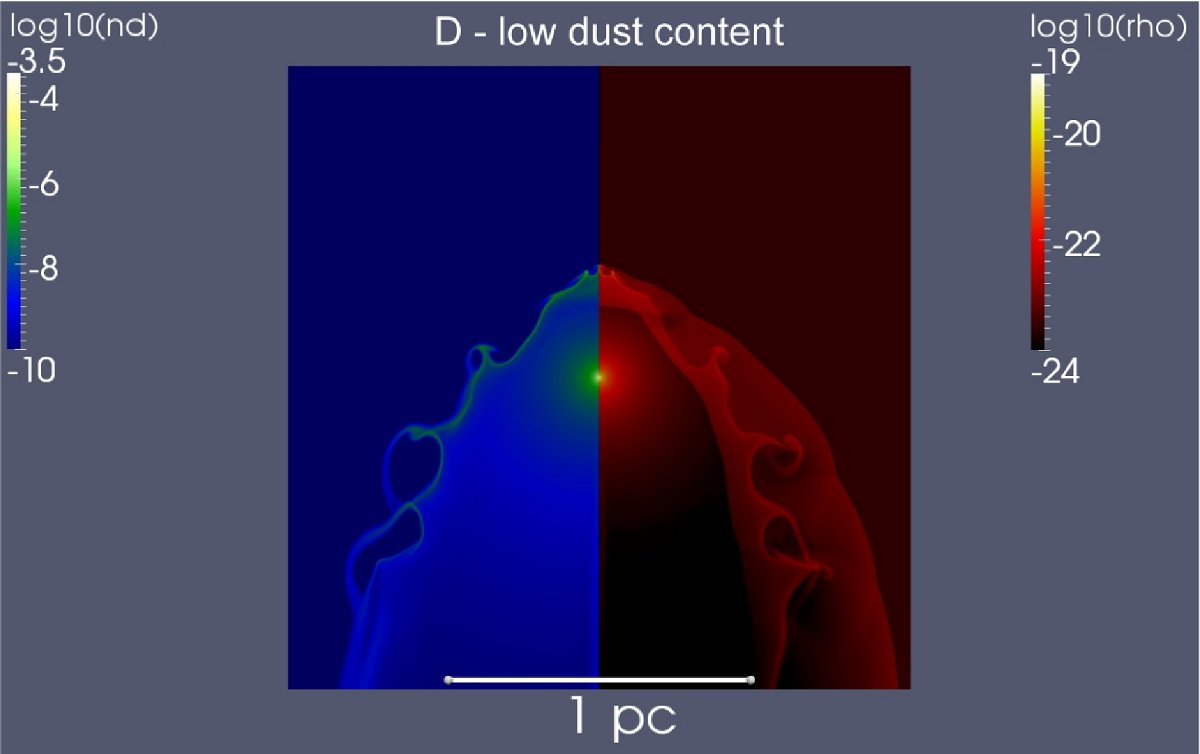
Figure 9: Similar to Fig. 8, but for simulation C after 1.0$\times 10^{5}$ years(top) and simulation D after 5.0$\times 10^{4}$ years (bottom). Top panel (C): Because of the weaker wind the bow shock is very close to the star. The bow shock morphology is completely stable. The shocked gas fills up the cavity behind the star due to low ram pressure of the wind, and thermal pressure of the shocked gas, because the shocks are almost completely adiabatic. Bottom panel (D): The bow shock is more conical than for the simulations with a stronger dust component and shows more instabilities. The instabilities are primarily of the Kelvin-Helmholtz type.

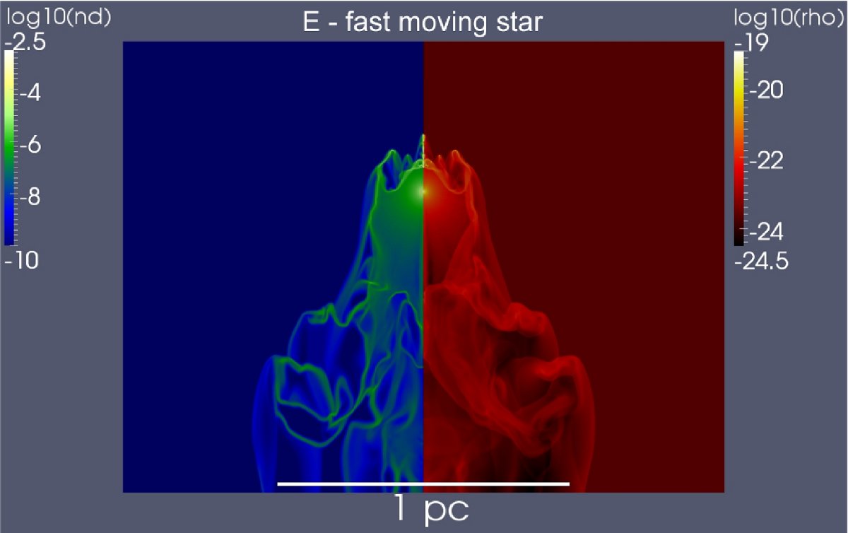
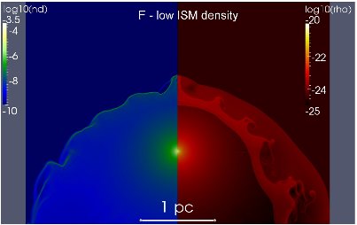
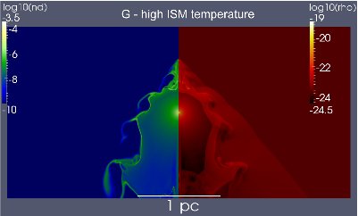
Figure 10: Similar to Fig. 8, but for simulation E after 6.5$\times 10^{4}$ years (top), F after 5.0$\times 10^{4}$ years (middle), and G after 1.0$\times 10^{5}$ years (bottom). Top panel (E): The entire shocked gas region is completely unstable due to a combination of radiative shocks and the high ram-pressure from the stellar motion in the ISM. The high ISM ram pressure brings the bow shock close to the star and the region behind the star is filled up with shocked gas due to the turbulent motion of the bow shock. Middle panel (F): The low density ISM results in a very extended bow shock region. Bottom panel (G): Due to the high ISM temperature, the radiative cooling in the shocked ISM is relatively ineffective. Since the shocked ISM maintains a high thermal pressure, due to the enforced minimum temperature of 8 000 K, the shocked gas fills the void behind the moving star.

6.2 The morphology of the bow shock

As shown in Figs. 8 through 10, the collision between the expanding wind and the moving (in the rest-frame of the star) ISM creates a bow shock. The location and morphology of the shocked gas depend on the exact input parameters. These figures show the gas density and dust particle density in the circumstellar environment after the bow shock has reached its (semi-) permanent equilibrium distance from the star. Typically, this takes between 50 000 and 150 000 years, depending on the parameters of the simulation. Our basic model (Simulation A, Fig. 8) shows a standard bow shock morphology: a forward shock separating the unshocked and shocked ISM, a wind termination shock that separates the free-streaming wind from the shocked wind, and between them a contact discontinuity separating the shocked wind from the shocked ISM, with the temperatures in the shocked wind typically lower than in the shocked ISM due to the higher density of the former. This pattern is repeated in all subsequent models, with the exception of the fast moving star (Simulation E, Fig. 10) and the high ISM temperature cases (simulation G, Fig. 10), both of which show a chaotic bow shock with strong turbulent behaviour.

Behind the star a relatively structureless – empty – region remains. This is only filled by the free-streaming wind of the star. Note that in our simulation the wind velocity is always less than the stellar velocity. Exceptions occur if the shocked gas region has a high thermal pressure, which pushes it into the empty region (Simulation C, Fig. 9 and simulation G, Fig. 10), or if the shocked gas is very turbulent (Simulation E, Fig. 10).

The location of the shock can be approximated by the wind and ISM conditions as described in Eq. 2. In Table 6 we give the location of the contact discontinuity ($R_{0}$) as well as the location of the forward shock of the shocked-gas region ($R_{s}$), where the ISM transition from unshocked to shocked gas is located. In some cases $R_{0}$ has to be approximated since instabilities can make it a time-dependent value. For simulation A (the basic model), the analytical approximation puts the contact discontinuity at 0.42 pc. In our simulation the position of the contact discontinuity deviates from this prediction, lying at about 0.26 pc (while the forward shock lies further ahead at $\sim$0.35 pc). The difference can be explained as a result of radiative energy loss in the shock. The scaling, as described by Eq. 2, appears to be quite accurate. For example, for an order of magnitude decrease in ISM density (simulation F, Fig. 10) or increase/decrease of mass-loss rate (simulation B, Fig. 8), the location of the bow shock moves away/closer with a factor of about $\sqrt{10}$.

The dust grains, which start with the same velocity as the wind, are initially carried along. When the wind reaches the termination shock, the gas slows down abruptly. Because they are not subject to the shock, the dust grains keep moving, but are now subject to drag force due to the difference in velocity with the gas. This causes them to slow down over time. As a result they tend to pile up at the contact discontinuity (van Marle et al. 2011b). Once the grains reach the contact discontinuity, they tend to follow the local instabilities and are eventually carried downstream. Those grains, which crossed the contact discontinuity, will usually go downstream faster, since in most of our simulations the shocked ISM has a higher velocity than the shocked wind. The influence of the grain size on the gas-dust interaction is investigated in van Marle et al. (2011b).

6.3 Instabilities in the bow shock

In most of our simulations, instabilities occur along the contact discontinuity. These instabilities consist of a combination of RT and KH effects (see above). In our case, the (relatively) low-density-shocked ISM exerts a force on the denser shocked wind, which leads to the formation of RT fingers. As a result, the wind material starts to flow into the shocked ISM. Here the wind material is subject to a sheer-force due to the relative motion of the star with respect to the ISM. These instabilities are enhanced by the dust (albeit this is a secondary effect), which tends to continue in a straight line in an attempt to cross from the shocked wind into the shocked ISM, dragging the gas along with it. This is best observed in the case of simulation B (Fig. 8). The velocity difference between the shocked gas layers causes KH instabilities to develop wherever the RT instabilities cause a local displacement of gas. These lead to the characteristic “cyclonic” features (see Figs. 8, 9 and 10). The presence of dust slows down the formation of KH instabilities, since the circular motion of the KH instabilities has difficulty overcoming the inertia of the dust grains. Therefore, they are most visible in simulation D (Fig. 9). Also, the KH instabilities can form more easily if the low density region (the shocked ISM) is extended, so that the instabilities do not hit the forward shock (simulation G, Fig. 10).

In the case of the star with a low mass-loss rate (simulation C, Fig. 9), such instabilities are absent. The low mass-loss rate leads to a reduced density in the shocked wind. As a result, the density difference between the shocked wind and the shocked ISM is small, which reduces the RT effect. Also, due to the low density, the radiative cooling, which scales with the density squared, is less effective (van Marle & Keppens 2011). This is important because radiative cooling tends to favor the formation of small, high density clumps, which in turn can serve as a start of other instabilities. Because the shocks are nearly adiabatic, the shocked-gas region is wide and its thermal pressure pushes material into the area behind the star, rather than leaving it empty.

The fast moving star (simulation E, Fig. 10) has a far more irregularly shaped bow shock. In this case the shocks on both sides are highly radiative, leading to a very compressed shocked gas region. This, combined with the strong ram-pressure from the ISM, causes the entire shell to become unstable, leading to a ragged form which will change considerable over time as local instabilities grow to a size where they dominate the entire structure of the shell. This turbulent motion also causes the gas (and the dust grains) to end up behind the star.

7 Discussion

7.1 Comparison between observed and hydrodynamical bow shock morphology

The simulations presented in Sect. 6 only cover part of the parameter space spanned by all stellar, circumstellar and interstellar properties. In particular, the simulations focus on the effects of increasing the star’s peculiar velocity with respect to the ISM, changing mass-loss rate, increasing the ISM temperature and lowering the ISM density.

One evident issue revealed by the simulation is that the shocked gas region can have considerable spatial extent (this occurs when the shocks are adiabatic - as in most cases presented here - as opposed to radiative). In the approximation of efficient cooling, the shock region will be thin and unresolved; however, the simulations show that this is not necessarily valid for all cases and can lead – depending also on the exact cooling law – to extended interaction zones. Depending on the exact morphology and the temperatures in the shocked gas region, one could – theoretically – be observing either the forward shock, reverse shock or contact discontinuity. However, the current far-infrared observations are most sensitive to cold dust grains. Due to the limited spatial resolution, it is not clear which region is actually represented by the far-infrared emission. It may represent the contact discontinuity (i.e. the entire unresolved shocked region), the bow shock, or the termination shock (Libert et al. 2007). Our simulations in Sect. 6 show that most dust grains pile-up at the contact discontinuity where they tend to follow the local instabilities which carry the grains downstream. Thus, the simulations suggest that the observed far-infrared dust emission primarily traces the contact discontinuity. On the other hand, if grains are destroyed in the shock they will be found in the unshocked stellar wind region and thus far-infrared dust emission would delineate the termination shock (and the contact discontinuity if the shock region is physically thin enough). This might prove useful in explaining the spatial offset between observed UV emission and far-infrared emission in the bow shock of CW Leo (Ladjal et al. 2010). Further work on the destruction and formation of dust grains (c.q. alteration of the dust size distribution) in shocks is warranted. As stipulated above, the simulations do not include radiative transfer and can thus not provide appropriate dust temperatures needed to simulate the infrared emission.

Table 7: Comparison between observed stand-off distances derived from Herschel/PACS maps and previous studies with IRAS, Spitzer & AKARI. The predicted values (this work) are given as a function of $n_{H}$ (cm^-3). The local interstellar ISM density, $n_{H}$, is estimated from the predicted $R_{0}/\sqrt{n_{H}}$ and the observed $R_{0}$ and compared to $n_{H}$ given by Eq. 5.

Object	De-projected $R_{0}$			Ref	$n_{H}$
	this work		literature		(cm-3)
	observed (′)	predicted (′)	(′)		Eq. 2	Eq. 5
$o$ Cet	1.2	0.7/$\sqrt{n_{H}}$	$\sim$3	(1)	0.4	1.1
$\alpha$ Ori	5.0	10.6/$\sqrt{n_{H}}$	$\sim$4	(2)	4.6	1.9
CW Leo	6.6	3.9/$\sqrt{n_{H}}$	5.9	(3)	0.3	0.7
R Hya	1.6	2.4/$\sqrt{n_{H}}$	1.6 $\pm$ 0.1	(4)	2.5	0.8
R Cas	1.5	2.2/$\sqrt{n_{H}}$	1.4 $\pm$ 0.1	(5)	2.1	1.8

References: (1) Raga & Cantó 2008; (2) Ueta et al. 2008, Decin et al. in preparation; (3) Ladjal et al. 2010, Sahai & Chronopoulos 2010; (4) Ueta et al. (2006); (5) Ueta et al. 2010

RT and KH instabilities

The presented PACS infrared observations reveal RT and KH instabilities in astrophysical bow shocks. RT fingers can be seen in the shock region of R Scl. KH “wiggles” or density knots are more common, and can be seen in the bow shock regions of, for example, UU Aur, R Hya, X Pav, EP Aqr, $\mu$ Cep, R Leo, RT Vir, X Her, and V1943 Sgr.

Almost spherical bow shocks spanning a large azimuthal angular range correspond closest to simulations A, B and F, the nominal, high $\dot{M}$ and low $n_{\mathrm{H}}$ cases, respectively. For low $n_{\mathrm{H}}$ (simulation F) the KH instabilities are more pronounced, while the RT instabilities are more evident in the high $\dot{M}$ case. The smooth, spherical bow shocks of $\alpha$ Ori, UU Aur, and X Pav are similar to the morphology of the simulation A (nominal case; Fig. 8). UU Aur and X Pav show back flow emission also seen in the simulation. The “wiggles” in the bow shocks of R Hya and R Leo correspond to those seen in simulation F (Fig. 10) which contradicts the high ISM density derived for R Leo (see Sect. 7.5). Both X Her and V1943 Sgr have high space velocities leading to morphologies much like that seen in simulation E (Fig. 10).

Further comparisons are hampered on the one hand by the (unknown) projection effects in the observations and on the other hand by the, currently, limited parameter space covered with the few simulations at hand. A more extensive, multi-parameter grid of simulations and/or a detailed modeling of individual cases will be required to match observations with simulations to confirm whether or not the latter accurately predict the former.

7.2 Proper motion and inclination

In most cases the proper motion vector (if known) points roughly (within $\sim$20°-30°) in the direction of the observed (Class I) bow shock apex. Exceptions are $\mu$ Cep and $o$ Cet. One possible explanation is that, like $o$ Cet, $\mu$ Cep is also a long-period (tens of years) binary, for which the present-day proper motion is not pointing in the same direction as it was when the bow-shock matter was expelled. This conjecture needs to be further tested by further observation and modeling of these systems and their observed bow shocks.

For the majority of the Class II objects, the proper motion direction is aligned roughly along the symmetry axis (perpendicular to the arc-star-arc line). Only for V Pav the proper motion points to the north-west arc. For Class IV the proper motion direction coincides with the location of extended irregular emission. The proper motion for Class III objects is not consistently aligned with, for example, shell features. In a few cases (TT  Cyg, U Ant) there is some stronger shell emission in the direction of the proper motion, but this is not observed for the other detected rings.

There is no clear indication for a dependency on the inclination angle, $i$. All five classes include sources with a range of inclinations between almost 0° up to 60-70°. Except for VY UMa ($i$=-1°), there are no objects with small inclination angles among the “eyes” (all have $i\geq 28$°), whereas the “fermata”, “rings” and “irregular” all have a more uniform distribution over inclination angles. However, we stress that at this point the sample is too small to derive any further conclusions.

For about one third of the “non-detection” class, the proper motions are not known and thus their space velocities are, at best, lower limits based on radial velocities. This is in part a distance bias. The objects with non-detections are on average further away and consequently their proper motions have been too small to be measured. This means also that the predicted stand-off distances are upper limits.

7.3 Binary interaction, circumstellar chemistry, and magnetic fields?

Binary interaction

There is little evidence for binary interaction in our sample. Even though for several stars in our sample, there is solid evidence for close companions (see Tables LABEL:tb:properties1 to LABEL:tb:properties2), none show suspicious features in their bow shock interfaces. However, many of these appear in the category “irregular”, which could indicate that such wind-wind-ISM interaction is only visible on small spatial scales. It is difficult to arrive at any firm conclusion as the number of binaries in the survey is low. Excluding the optical “visual” binaries, as these are not yet confirmed, out of the 25 objects in the “fermata” class only one is a known binary (Mira) which indeed reveals a peculiar shape of the interaction zone (Mayer et al. 2011). Three others, W Aql, EP Aqr and $\theta$ Aps are solid candidates for binarity. None of the “rings” are binaries. Noteworthy, 3 out of 6 of the “irregulars” are confirmed binaries, and 2 of the 6 “eyes” are potentially binaries. Finally, also 6 out of 30 non-detections are binary systems. Including visual binaries adds 3 binaries to each of the “fermata”, “eyes”, and “non-detection” classes, and 4 binaries to the “rings”. In this case, 5 out of 7 “eyes” show evidence for binarity, whether this means there is a connection between binarity and the “eyes” morphology can not be confirmed nor excluded at this point.

Oxygen-rich versus carbon-rich chemistry

One key property of the AGB stars and red supergiants in our sample is their circumstellar envelope chemistry. This can be either carbon-rich (the dust is predominantly made up of amorphous carbon, graphite and silicon carbide) or oxygen-rich (the dust is composed of silicates and oxides). Although we do not find a strong dependence on the presence versus absence of bow shocks and rings with respect to chemistry, there does appear to be a distinction between the shape of the extended emission found around carbon and oxygen-rich objects. The “fermata” and “irregular” classes include a high fraction, 22 out of 31, of O-rich stars. The “eyes” and “rings”, on the other hand, include only few, 3 out of 22, O-rich stars. It seems that at least the “ring” structure is typical of C-rich chemistry, as already pointed out by Olofsson et al. (2000). A further argument favoring such a link between “ring” structure and C-richness is that all “fermata” stars also displaying a “rings” structure are C-rich stars (they are noted with an asterisk in Table LABEL:tb:properties1, and are also listed in Table LABEL:tb:properties2).

Could the circumstellar envelope structure be related to chemistry through differences in mass loss rates? It has been shown (Knapp 1985) that oxygen-rich stars have a wider range of mass-loss rates than C-rich stars for which the $\dot{M}$ is globally more homogeneous. On average, mass loss rates of C stars are higher than those of MS and S stars (Guandalini 2010). Apart from the fact that the mass-loss rate standard deviation of O-rich stars is indeed found to be somewhat larger than that of C-rich stars, no clear dichotomy emerges between the mass loss rates of O-rich stars and C-rich stars in the present sample.

Furthermore, the higher emissivity (Draine & Lee 1984; Li & Draine 2001) and lower gas-to-dust ratio of 160 for oxygen-rich dust compared to the higher ratio of 400 for carbon-rich dust (see e.g. Knapp 1985; Heras & Hony 2005) will, for O-rich dust, give rise to brighter infrared emission for a given total dust and gas mass. One could then argue that the O-rich stars mass loss is more easily detected even with a patchy structure. This could perhaps explain why O-rich stars are detected preferentially among both “irregulars” and “fermata” classes.

An alternative explanation is that the “Ring” (and possible the “Eyes”) morphology, are explained through (i) the interaction between a fast wind sweeping out matter from a previous slower wind, or (ii) a phase of drastically enhanced mass loss, e.g. caused by a thermal pulse. If this explanation holds, and if one assumes that most thermal pulses events are followed by a third dredge-up (TDUP) episode, then the discriminant character would not be O-rich or C-rich, but instead pre-TDUP or post-TDUP (i.e., thermally-pulsing (TP) AGB) stars). All intrinsic S-type stars, C-type stars and technetium-rich M stars in Tables LABEL:tb:properties1 and LABEL:tb:properties2 are TP-AGB stars. In fact, all “Ring” stars are TP-AGB stars.

Stellar and interstellar magnetic fields

Some wind-ISM models include the effects of an interstellar magnetic field on the shaping of the bow shock region. Heiligman (1980) predicted that the ISM magnetic pressure could deform the outer shells of very large spherical halos of PNe into “lemon” shapes, with the axis of symmetry inclined to the ordered ISM magnetic field direction. Soker & Dgani (1997) and Dgani (1998) elaborated on this scenario predicting different bow shock shapes depending on the relative magnitudes of the star’s space velocity, $v_{\star}$, the wind velocity, $v_{w}$, and the Alvén speed, $v_{A}$. The double arc objects (Class II) such as VY UMa and AQ Sgr could perhaps provide evidence for this scenario, although both are at relatively high latitudes and their symmetry axes are not aligned with the Galactic plane (assuming that at these locations the magnetic field is also parallel to the Galactic plane). It is also possible that the star has its own magnetic field and thus may exhibit axis-symmetric mass loss. Preliminary simulations (private communication A.-J. Van Marle) indicate that double arcs as well as jets (tentatively identified for VY UMa and W Hya) could be formed by a (rotating) star with a magnetic field.

7.4 Detached spherical shells

The observed detached shell objects (Class III) show quite a range of expansion ages calculated out of their measured or assumed expansion velocities, distances and angular sizes. Ranging from the youngest shells like U Cam or R Scl with ages of the order of 1000 years and much older ones like AQ And, Y CVn or UX Dra with ages of a few 10 000 years we see also a significant trend in the detectability in fossil mm-CO. Whereas all objects with shell ages below some 1000 years are prominent in CO, no detached shell older than 10 000 years was successfully detected yet. This could be understood in terms of photo-dissociation by the interstellar radiation field in the older extended shells with sizes of 0.2 pc or more (Kerschbaum et al. 2010). Arimatsu et al. (2011) find that the detached shell of U Ant detected with PACS is not the outermost one found with AKARI. Thus, the shell detected with PACS is either a density enhancement due to a two-wind interaction or it could represent the termination shock, similar to the scenario proposed for Y CVn by Libert et al. (2007).

Another interesting finding with respect to Class III objects are the objects that have both a detached shell and a bow shock interaction region, with R Scl being the showcase object. Seeing the bow shock far out off the detached shell more or less excludes one of the explanations of detached shells, namely their interpretation as being the wind-ISM interface (Libert et al. 2007).

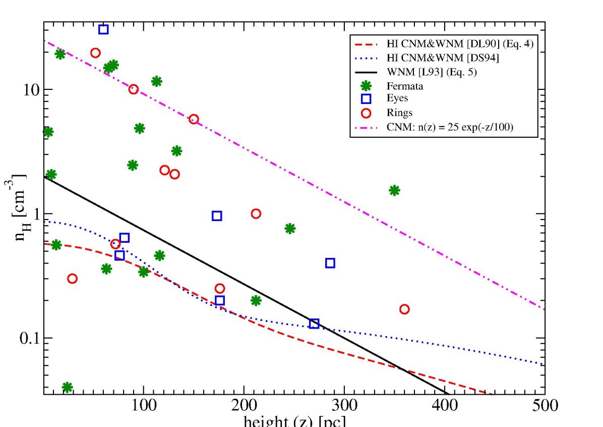
Figure 11: ISM density derived from the observed stand-off distance $R_{0}$ as a function of the height above the Galactic plane, $z$. Different density scaling height models are also shown (e.g. Eqs. 4 and 5). References: [DL90]: Dickey & Lockman (1990); [DS94]: Diplas & Savage (1994); [L93]: Loup et al. (1993).

7.5 Comparison between predicted and observed $R_{0}$: Implications for the ISM density

For a number of objects in our sample, previous studies have reported on the detection of wind-ISM bow shocks with IRAS, Spitzer or AKARI. The measured deprojected angular stand-off distance obtained with PACS agree very well with earlier results (Table 7). The predicted values for $R_{0}$ (as function of $\sqrt{n_{H}}$) give ISM densities that are somewhat higher than those computed from Eq. 5. For $\alpha$ Ori, Ueta et al. (2008) predict $n_{\mathrm{H}}$ = 1.5 – 1.9 cm^-3 which is indeed in line with $n_{\mathrm{H}}$ = 1.9 cm^-3 derived from Eq. 5, but higher than that inferred from the stand-off distance, $n_{\mathrm{H}}$ = 4.6 cm^-3 (Table 7). Ladjal et al. (2010) derive $n_{H}\geq 2$ cm^-3 for CW Leo, which is a factor of 2 higher than derived from both our predicted stand-off distance as well as from Eq. 5 ($n_{\mathrm{H}}$ = 0.5 – 1.0 cm^-3).

Adopting the values for the different parameters given in Tables LABEL:tb:properties1 to LABEL:tb:properties2 yields $R_{0}$ less than 8′ for all objects with detected bow shock interaction. For all detected wind-ISM interaction objects, the predicted stand-off distances range from about 0.02 to 0.9 pc, in line with the observed de-projected values. This gives some credibility in the predicted stand-off distances (from Eq. 2) for the objects in Class X (“non-detections”). These results suggest that additional bow shocks should have been detectable for other stars within 300 pc, in particular for R Dor, Y Lyn, RS Cnc, and possibly HD 100764 and RX Boo. We note that higher sensitivity observations could possibly still reveal the expected extended emission.

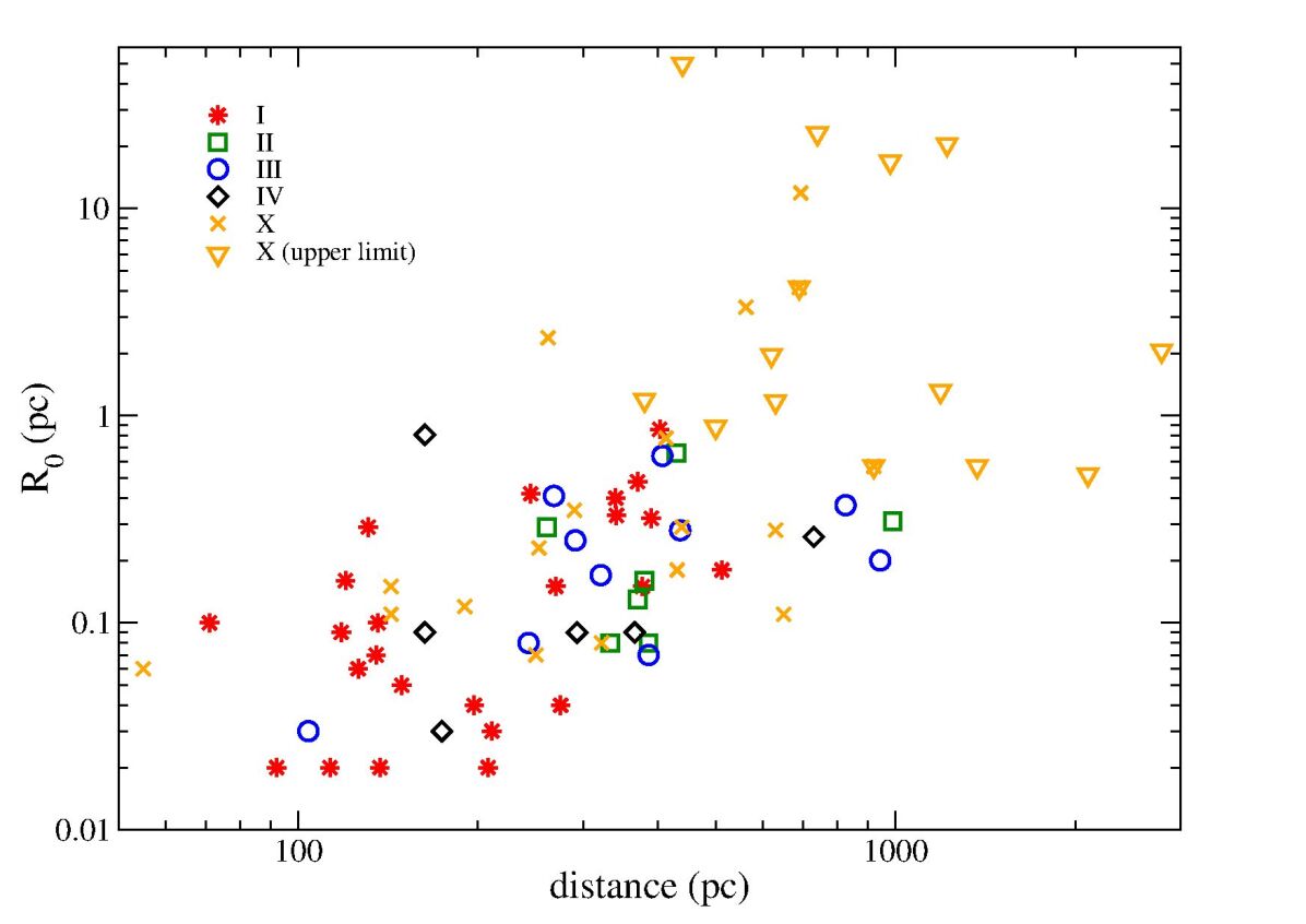
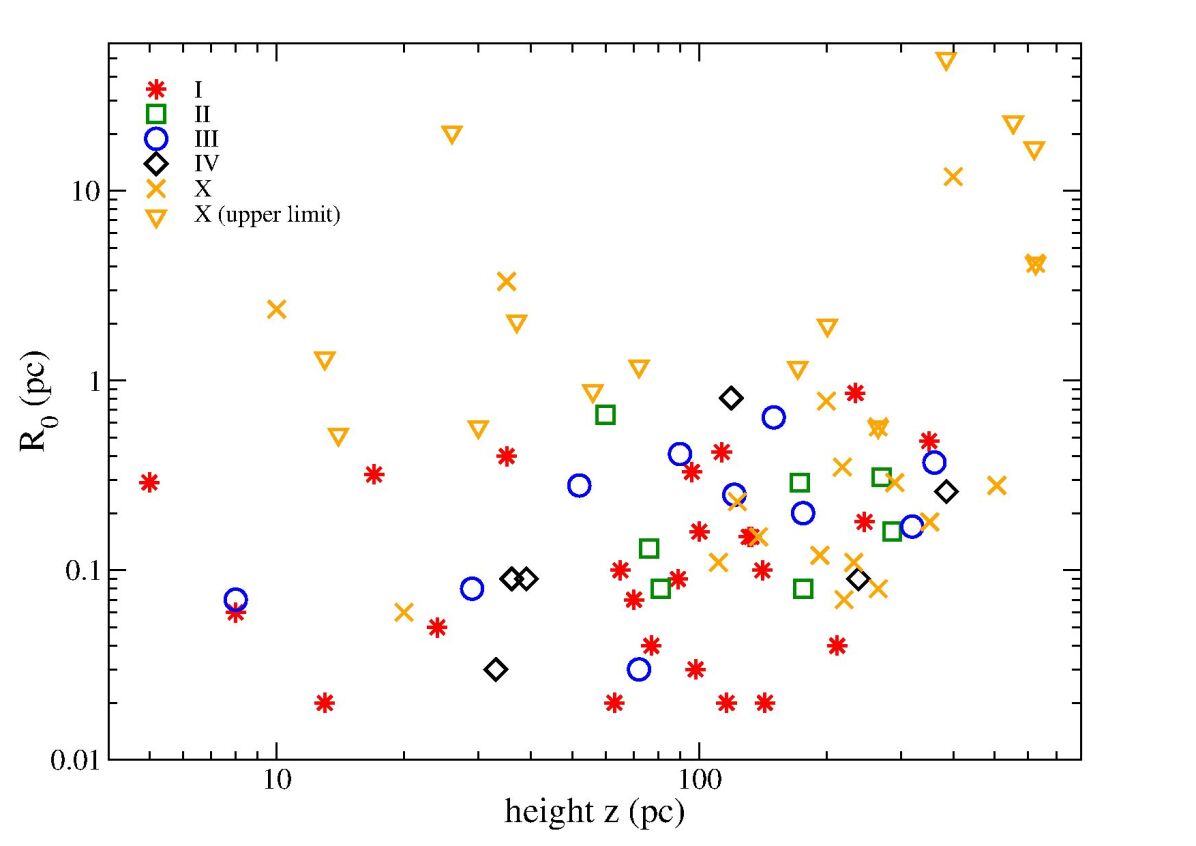
Figure 12: Predicted stand-off distance as a function of distance (top) and as a function of height above the Galactic plane, $z$ (bottom). All in units of parsec. Classes: I (stars), II (squares), III (circles), IV (diamonds), and X (crosses & triangles).

The uncertainty of the predicted stand-off distance depends on the different stellar and ISM parameters. The space velocity, $v_{\star}$ (for nearby stars), as well as the wind velocity, $v_{w}$ are well determined observationally with small ($\sim$10%) uncertainties. The uncertainties in the mass-loss rates can be an order of magnitude, in particular for the targets with inaccurate distance estimates (Sect. 5) which introduces errors of a factor of three in $R_{0}$. Finally, the local ISM density is difficult to derive observationally. Without knowledge of the exact phase of the ISM the star is traversing, estimates of the density could be off by several orders of magnitude (see the discussion on densities, scale heights, and filling factors in Sect. 5). Table LABEL:tb:properties1 lists $n_{\mathrm{H}}$ derived from equating the observed de-projected $R_{0}$ with the theoretical $R_{0}$, taking $n_{\mathrm{H}}$ as the unknown. The comparison of $n_{\mathrm{H}}$ derived from Eq. 5 with that derived from the observed and predicted $R_{0}$ shows that these generally agree within a factor of three (Fig. 11). In a few cases, the derived ISM density is an order of magnitude higher ($n_{H}\approx 5$ to 35 cm^-3) than given by Eqs. 4 and 5. Possibly, for these cases, the star is moving through a diffuse cold medium (CNM) with typical densities $n_{H}\sim 10-100$ cm^-3, an order of magnitude higher than those of the WNM (Sect. 5). Alternatively, this apparent discrepancy could also be resolved if the ISM itself has a peculiar flow velocity of $v_{\star}$-$v_{\rm ISM}$ with respect to the local standard of rest. If the peculiar velocity between the two media is higher, the density required to arrive at the same stand-off distance is lower, since $v_{\star}\propto 1/\sqrt{n_{H}}$. On the other hand, the derived ISM density also scales linearly with the adopted $\dot{M}$, thus an order of magnitude over-estimate of the mass-loss rate leads to the same order of magnitude over-estimates of $n_{\mathrm{H}}$. This may explain the high $n_{\mathrm{H}}$ for some objects with high adopted $\dot{M}$, such as W Aql, but not easily for others, such as R Leo, which have already low values for $\dot{M}$. For R Leo, the turbulent features in the bow shock indicate a higher space velocity which is at odds with the observed $v_{\star}=15$ km s^-1. If indeed the relative star-ISM space velocity for R Leo is higher, the inferred ISM density will be correspondingly lower (now $n_{H}\propto v_{\star}^{-2}$). For example, for a much higher peculiar velocity of 45 km s^-1  (more in line with the bow shock morphology), $n_{H}=1.6$ cm^-3 which is close to $n_{H}=1.1$ cm^-3 given by Eq. 5. In Sect. 5 we roughly estimated the LSR velocity of the local ISM and found that the corrections to $v_{\star}$ are small ($\leq$ 20%) for most objects, with a few exceptions. Only for two cases do these higher relative velocities lead to much smaller values for the ISM density; $n_{\mathrm{H}}$ = 10.1 and 13.5 cm^-3 for $\mu$ Cep and U Cam, respectively. The ISM velocity correction does not alter the high densities obtained for e.g. R Leo, W Aql and EP Aqr. Another explaination could be that this ‘denser’ medium is a remnant of an earlier, slower stellar wind. How and if the (tentative) binarity of both W Aql and EP Aqr plays a role is as of yet not clear.

7.6 Presence versus absence of wind-ISM bow shocks

In the previous sections, we have established different morphological classes of bow shocks and examined the basic physics giving rise to a bow shock and discussed the various parameters affecting their size and shape. In this section we explore different properties of the stellar objects as well as the ISM in order to understand which conditions are required to be able to detect bow shocks and/or detached shells around AGB stars and red supergiants.

For 50 out of 78 (63%) AGB stars and red supergiant, we detect detached extended far-infrared emission suggestive of a bow shock, detached ring or irregular extended emission. Limiting the sample to nearby objects ($d\leq 500$ pc) eliminates many uncertainties and the “detection-rate” improves to 43 out of 56 objects, or 78%. Restricting the distance further to, for example, $d\leq 300$ pc, only marginally improves the detection rate to 28 out of 34 (80%).

To test whether the “detection” and “non-detection” samples have similar or statistically different distributions as a function of $d$, $z$ or $n_{\mathrm{H}}$, $v_{\star}$, $i$, $\dot{M}$, and $R_{0}$, we use the two-sample Kolmogorov-Smirnov ($K$-$S$) test. The results are given in Table 8. In order to eliminate the effect of large uncertainties in the distances, we perform the $K$-$S$ test on a distance limited ($d\leq 500$ pc) sample. The $K$-$S$ probabilities of “detections” versus “non-detections” are particularly low (and thus indicative that the two samples have different distributions) for $n_{\mathrm{H}}$/$z$, $v_{\star}$, and $R_{0}$. The corresponding distribution histograms for the most distinctive parameters, $n_{\mathrm{H}}$, $v_{\star}$, and $R_{0}$, are shown for the different classes (detection/non-detection) in Figs. 13 to 15. This points towards the scenario that the presence of bow shocks is strongly dependent on the stellar velocity (relative to the local medium), the local ISM density and the resulting standoff distance. The latter sets the size of the bow shock region and is apparently determined predominantly by $v_{\star}$ and $n_{\mathrm{H}}$ and not so much by the star’s mass-loss properties (cq. evolutionary phase).

All objects with observed wind-ISM interaction zones (Class I to IV) have $R_{0}$ $\leq$ 1 pc, while many class X sources have $R_{0}$ $\geq$ 1 pc. The distribution of the observed de-projected $R_{0}$ values is very similar to the distribution of predicted $R_{0}$ for sources in Class I to IV. However, a quantitative comparison between the predicted and observed stand-off distances does not reveal a strong correlation.

Irrespective of the absolute distance (and thus apparent angular stand-off distance) it appears that a necessary, but not sufficient, condition for the detection of bow shocks and rings is that their physical size has to be smaller than about 1 pc. This points towards a physical effect (e.g. reduced surface brightness) instead of an observational limit, although it does not explain the absence of bow shock emission around nine of the observed nearby AGB stars (with known $v_{\star}$ and $R_{0}<1$pc) included in Class X.

Concluding, we find that bow shocks are detected and predicted to occur for most nearby objects ($<$ 500 pc) as well as for objects whose stellar and local ISM properties yield relatively small stand-off distances ($<$ 1 pc). For more distant objects the detection is (likely) hampered by lower sensitivity and lower spatial resolution, though we could not find any reasons to suggest that these objects would not have bow shock interaction. Indeed, several distant objects such as AQ And ($\sim$800 pc), S Cas ($\sim$940 pc), RZ Sgr ($\sim$730 pc) reveal evidence for wind-ISM interaction, but these detections might have been fortuitous.

Table 8: Two-sample Kolmogorov-Smirnov test applied to different stellar, circumstellar and interstellar parameters possibly relevant to “detection” and “non-detection” samples (distance $d\leq 500$ pc).

	Kolmogorov probability $p$
	(I,II,IV)	(I,II,IV)	(III)	(I-IV)
	vs. (III)	vs. (X)	vs. (X)	vs. (X)
	n=(34,8)	n=(34,16)	n=(8,16)	n=(42,16)
critical value ($\alpha=0.01$)	0.70	0.56	0.76
$d$ (pc)	0.25	0.18	0.98	0.28
$z$ (pc) / $n_{H}$ (cm-3)	0.99	0.03	0.19	0.02
$v_{\star}$ (km s-1)	0.43	0.02	0.09	0.02
inclination $i$ (°)	0.01	0.52	0.19	0.68
$\dot{M}$(M⊙ yr-1)	0.55	0.48	0.59	0.57
$v_{w}$ (km s-1)	0 78	0.74	0.84	0.78
$R_{0}$ predicted (pc)	0.40	0.07	0.84	0.09
$R_{0}$ predicted (arcmin)	0.94	0.02	0.19	0.02

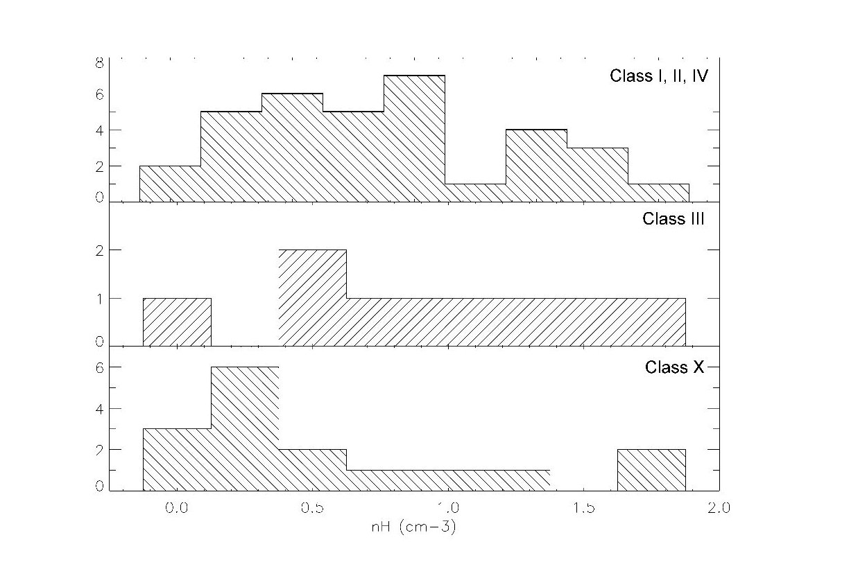
Figure 13: Histogram of the “predicted” ISM density, $n_{\mathrm{H}}$, for the “detected” Class I, II, IV (top panel) and Class III (middle panel) “non-detection” Class X (bottom panel) objects.

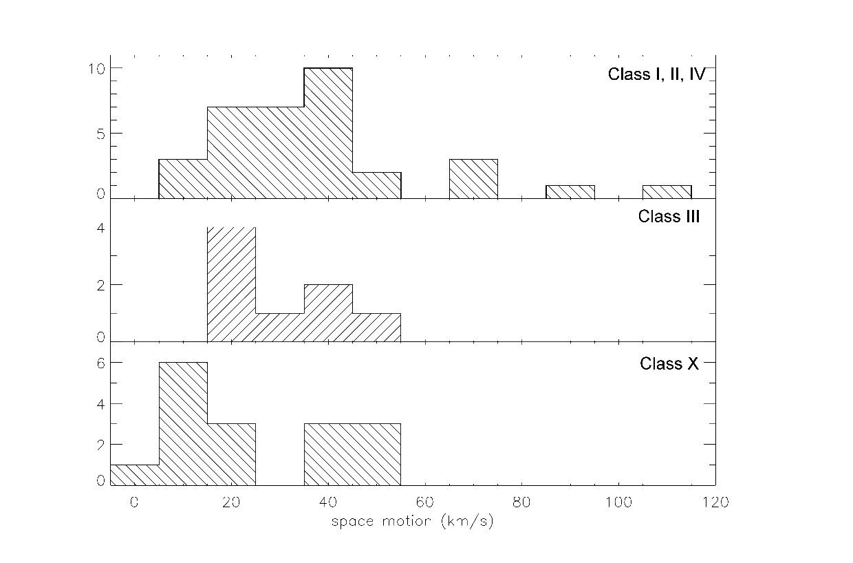
Figure 14: Histogram of the space velocity, $v_{\star}$, for the “detected” Class I, II, IV (top panel) and Class III (middle panel) “non-detection” Class X (bottom panel) objects.

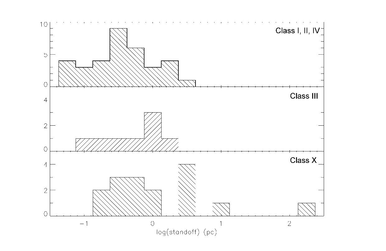
Figure 15: Histogram of the standoff distance, $R_{0}$ (pc), for the “detected” Class I, II, IV (top panel) and Class III (middle panel) “non-detection” Class X (bottom panel) objects.

8 Conclusions

This paper presents a morphological inventory of “wind-ISM” bow shocks and “wind-wind” interactions detected in the far-infrared with Herschel/PACS. Five main classes are identified:

• “Fermata”. These objects are characterised by a large arc or shell-like structure spanning an angle of at least 90°. Several objects in this class show the presence of turbulence, i.e. Rayleigh-Taylor or Kelvin-Helmholtz instabilities. Some objects, such as X Pav, EP Aqr, and X Her, reveal the presence of back flowing material in the wake (behind) the star, leading to a distinct bullet-shape.

• “Eyes”. These are characterised by two arcs on opposing sides of the central object. These arcs are elliptical and non-concentric. In two cases the arcs connect and form a “lemon” shape morphology.

• “Rings”. This class includes the well known detached shell objects, typical of wind-wind interaction and dust pile-up. Younger, smaller rings have a co-spatial counterpart molecular gas ring, while the larger dust shells do not.

• “Irregular”. This class includes all sources which show extended (non-detached), irregular emission at 70 or 160 $\mu$m.

• “Non-detection”. All objects for which no large extended far-infrared emission has been observed (c.q. resolved) in the form of a bow shock or ring with the PACS instrument.

Oxygen rich stars give rise predominantly to “fermata” or “irregular” morphologies. There is tentative evidence that all “ring” stars are thermally-pulsing AGB stars. We identify a few cases for which both a detached (inner) shell is found within the (outer) bow shock, suggesting that the detached shell is not due to the wind-ISM interaction, but suggest rather a wind-wind scenario.

The presence or absence of bow shocks is determined by the stand-off distance which depends on relative values of the stellar parameters ($v_{\star}$, $v_{w}$ and $\dot{M}$) as well as those of the ISM ($n_{\mathrm{H}}$) as given by the theoretical approximation as well as the hydrodynamical simulations. The distribution of stand-off distances for the entire survey sample shows a clear separation between objects with and without detected extended emission. Indeed most of the objects (44) assigned to Classes I to IV have $R_{0}<$ 1.0 pc. No extended bow shock or detached shell emission has been detected for the 15 objects with predicted $R_{0}>1$ pc and/or $d>1000$ pc. Limiting the sample to $d<500$ pc, we derive a $R_{0}<1.0$ pc, and thus predict the presence of bow shocks, for 8 stars in the “non-detection” class: TW Hor, V Eri, R Dor, R Lep, RS Cnc, HD 100764, RY Dra, and RX Boo. Many of these show extended shells at about 1 MJy sr^-1 sensitivity in Spitzer and AKARI maps (private communication: T. Ueta for Spitzer and H. Izumiura for AKARI).

The angular size of the predicted stand-off distances for 6 other objects in Class X are larger than the obtained PACS image maps. In particular, all-sky survey missions, such as AKARI (Murakami et al. 2007) and WISE (Wright et al. 2010) could help in observing extended bow shocks and shells around these objects. Observations of bow shocks and detached shells for distant ($>$1 kpc) AGB stars and red supergiants require thus higher sensitivities to detect extended emission, but not necessarily higher spatial resolution as most have predicted stand-off distances larger than 1′.

The observed infrared emission indicates the presence of moderate amounts of dust ($2\times 10^{-7}$ to $2.5\times 10^{-4}$ M_⊙), implying only up to a few tenths of solar masses of dust and gas in the bow shock interaction region. The observed dust and gas masses are similar to the potentially swept-up ISM material.

This survey represents only a first step in fully characterising and understanding the formation and shaping of bow shocks and detached shells around AGB stars and red supergiants. It is clear that additional simulations trying to represent as closely as possible the different observed morphologies are required in particular to understand the formation of instabilities. Detailed observations of the bow shock spectral energy distribution (dust) and line emission (gas) is needed to quantify the physical conditions and composition of the material in these shocked regions. Potentially, detailed observations of bow shocks around larger samples of AGB stars can be used to independently probe the local ISM density (and possibly the magnetic field) distribution in the Galaxy.