Mechanism for flux guidance by micrometric antidot arrays in superconducting films

Abstract

A study of magnetic flux penetration in a superconducting film patterned with arrays of micron sized antidots (microholes) is reported. Magneto-optical imaging (MOI) of a YBa₂Cu₃O_x film shaped as a long strip with perpendicular antidot arrays revealed both strong guidance of flux, and at the same time large perturbations of the overall flux penetration and flow of current. These results are compared with a numerical flux creep simulation of a thin superconductor with the same antidot pattern. To perform calculations on such a complex geometry, an efficient numerical scheme for handling the boundary conditions of the antidots and the nonlocal electrodynamics was developed. The simulations reproduce essentially all features of the MOI results. In addition, the numerical results give insight into all other key quantities, e.g., the electrical field, which becomes extremely large in the narrow channels connecting the antidots.

I Introduction

The motion of magnetic flux in type-II superconducting films can to a large extent be controlled by introduction of artificial micro- and nano-structures, such as antidots (holes),Baert et al. (1995); Eisenmenger et al. (2001); Pannetier et al. (2003) magnetic dots,Martín et al. (1997); Gheorghe et al. (2008) thickness modulations,Ivanchenko and Mikheenko (1983); He et al. (2009) grain boundaries,Polyanskii et al. (1996); Bartolomé et al. (2007) slits,Baziljevich et al. (1996) or magnetic domain walls in superconductor/ferromagnet hybrids.Goa et al. (2003a); Vlasko-Vlasov et al. (2008) Such structures are key building blocks for successful realization of fluxonics devices like vortex ratchets, pumps and lenses etc.Villegas et al. (2003a); de Souza Silva et al. (2006); Wambaugh et al. (1999) It is known that when antidots are sufficiently small they can become pinning sites for the vortices.Mkrtchyan and Shmidt (1972) This type of pinning is usually noticable only close to the critical temperature $T_{c}$, and can be observed, e.g., as pronounced matching between the vortex density and the underlying lattice of antidots.Moshchalkov et al. (1998); Silhanek et al. (2003) It was also demonstrated that certain patterns can be used to reduce noise due to vortex motion in SQUIDs,Wördenweber and Selders (2002) and quite recently in superconducting microwave resonators.Bothner et al. (2011)

Of technological as well as fundamental interest is also realizations of flux guidance, i.e., how to achieve directed and controlled motion of the magnetic flux. When the pinning by the antidots is strong compared to the intrinsic pinning of the material, guidance is effectuated by the more mobile interstitial vortices.Reichhardt and Olson Reichhardt (2009) Conversely, when the intrinsic pinning is strong, flux moves most easily inside the holes, and arrays of antidots should enhance the flux penetration.Vestgården et al. (2008) It has been shown that by introducing arrays of dotsVillegas et al. (2003b) or antidotsSilhanek et al. (2003); Wördenweber et al. (2004) the vortices can be guided away from the direction given by the Lorentz force of an applied current. Similarly, a periodic arrangement of antidots can cause effective flux drainage of a sample in the descending branch of a magnetic field ramp.Crisan et al. (2005) It was also found that when the antidot lattice breaks the symmetry of the overall sample shape, or when the antidots have nontrivial shapes, the critical current density can become anisotropicPannetier et al. (2003); Gheorghe et al. (2006) and the flux motion can be enhanced in unexpected directions.Tamegai et al. (2010)

Whereas superconducting films containing complex arrangements of antidots can today be readily produced using, e.g., optical lithography, the theoretical modelling of the local and global features of the flux dynamics in such systems is challenging. In essence, this is due to the nonlocal nature of the electrodynamics in two-dimensional samples subjected to a perpendicular magnetic field. In this case the critical-state is strongly modified since at any applied field there will be currents flowing over the whole sample area, including regions in the flux-free Meissner-state.Norris (1969); Brandt and Indenbom (1993); Zeldov et al. (1994) Also numerical simulations of the flux dynamics are a lot more computationally demanding in films compared to bulk.Brandt (1995); Lörincz et al. (2004); Vestgården et al. (2011) Additional complications appear in a film with antidots, as the shielding currents then meet constrictions, and the flow must adapt to the available and often narrow bridges of superconducting material between the antidots. Hence, the current density quickly rises to the critical value, causing major rearrangements of both the current flow and the flux distribution.Vestgården et al. (2008)

Magneto-optical imaging (MOI) is a unique experimental tool for observing the nontrivial redistributions created by patterning of superconducting films. The technique allows direct observation of the flux density over length scales ranging from the entire sample size and down to the size of individual antidots. In spite of large previous efforts, surprisingly few investigations were carried out on films with simple antidot patterns. In this work we present results from MOI experiments together with theoretical modelling of the flux and current behavior in a thin superconducting strip containing only a few linear arrays of antidots. The experiments were performed using a film of YBa₂Cu₃O_x (YBCO) cooled far below $T_{c}$ to be in the regime where flux pinning by the antidots is negligible.

The paper is organized as follows. In Sec. II we outline the current flow modification caused by an antidot array as expected from the critical state model. Section III presents results from our MOI experiments. Section IV describes our method for numerical simulations of the electrodynamics, and the results are presented and discussed in Sec. V. Section VI gives a summary.

II Critical current flow lines

Before presenting the experimental results we consider the predictions of the Bean critical-state model for a type-II superconducting strip with a linear array of equally spaced antidots crossing from one side to the other, see Fig. 1. The antidots have radius $r$ and center-to-center distance $a$. An external magnetic field, $H_{a}$, is applied perpendicular to the strip plane, and we assume the superconductor initially contains no flux and current.

As the field is gradually increased magnetic flux will penetrate from the edge and shielding currents will begin to flow. In areas containing flux, the critical state is formed and the current density has the critical magnitude $j_{c}$, while in the unpenetrated Meissner-state region the currents have a subcritical density. To draw the current stream lines in the critical-state region we use the simple rule following from the Bean critical-state model, namely that the magnitude of the current density is constant, and thus represented by a set of equidistant stream lines with spacing inversely proportional to $j_{c}$. The construction starts by drawing continuous lines that follow the external perimeter of the sample, and when reaching a hole the current must flow around it. This scheme results in the flow pattern shown in the Fig. 1, corresponding to a partly penetrated state. The closure of each streamline takes place in parts of the sample not included in the figure.

The figure shows that the presence of the antidot array deforms the critical current in a large region with a near rhombic shape. A line denoted d-line₁ marks where the direction of the current flow suddenly begins to deviate from being parallel to the edge. Using the principle of current flow continuity one finds that the line makes an angle $\alpha$ with the edge, given by

$$\cos\alpha=\sqrt{r/a}\ .$$ (1)

Evidently, such a line exists on both sides of the array, and the pair defines one half of the rhombic area.

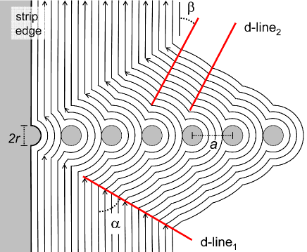
Figure 1: (Color online) Construction of the critical current streamlines near a linear array of equidistant circular antidots. The pattern follows from the Bean critical-state model for a sample with a straight edge. Note that streamlines of the sub-critical currents flowing in the Meissner-state part of the strip are not included.

In addition to the large perturbation of the current flow, the construction also results in a fine structure in the flow pattern. Due to the shape of the antidots the stream lines inside the rhombic area consist of a sequence of circular arcs. As seen from the figure, each antidot creates its own pair of lines along a direction defined by the cusped joints of two arcs. These lines, denoted d-line₂, become straight a short distance from the array, and one finds that the angle, $\beta$, they make with the strip edge is the same for all of them, and given by

$$\cot\beta=2\frac{\sqrt{r(a-r)}}{a-2r}\ .$$ (2)

Related to this construction is a previous analysis of the current flow in the case of having a weak link across the superconducting strip.Polyanskii et al. (1996) It was assumed that inside the weak link the critical current density is uniformly reduced by a factor $j_{b}/j_{c}$. Also that construction resulted in a rhombic area where the current has changed direction, and the angle $\alpha$ was found to be given by $\cos 2\alpha=-(j_{b}/j_{c})$. Indeed, this is equivalent to Eq. (1) with the transparency of the antidot array, $(a-2r)/a$, replaced by the current ratio in the weak link case.

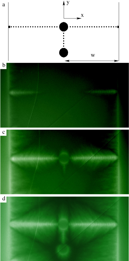
Figure 2: (Color online) Sketch of the antidot arrangement in the superconducting sample, which has an overall shape as a long thin strip in the $xy$-plane (a). The flux distribution, $B_{z}$, in the YBCO film seen by MOI and recorded at applied fields of 2.4 mT, 5.7 mT and 10 mT, respectively (b-d).

III Experiment

A 150 nm thick YBCO film was produced by magnetron sputtering on a r-cut sapphire substrate. The sample was shaped using optical lithography and ion beam etching into a long strip 0.5 mm in width, and with an arrangement of antidots as shown in Fig. 2a. The antidots having radius $r=2~{}\mu$m form a linear array with period $a=10~{}\mu$m. Along the center line there are two larger antidots of radius $20~{}\mu$m, connected with an array of 6 antidots, also of radius $r=2~{}\mu$m. The arrangement was motivated by a possibility to study flux guidance along linear antidot arrays both perpendicular and parallel to the strip edges. The large holes are included to serve as reservoirs for the incoming flux.

Magneto-optical imaging of the sample was performed using a bismuth substituted ferrite garnet film with in-plane magnetization as Faraday rotating sensor.Helseth et al. (2001) Images of the flux distribution were recorded through a polarized light microscope using crossed polarizers. In this way the image brightness represents the magnitude of the flux density. For details of the setup, see Ref. Goa et al., 2003b.

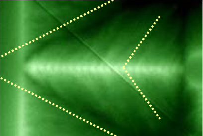
Figure 3: (Color online) Details of Fig. 2 showing the d-line pattern from a row of antidots. The straight d-line₁ and d-line₂ are drawn as a guide to the eye with angles corresponding to Eqs. (1) and (2) calculated for the geometrical characteristics of the antidot array in the YBCO film.

Shown in Fig. 2b-d is the flux distribution, $B_{z}$, in the patterned part of the sample as the applied field is slowly ramped up to $\mu_{0}H_{a}=10$ mT after an initial zero-field-cooling to 50 K. As typical for thin films, the rim of the strip appears bright, thus showing piling up of the field that is expelled by the superconductor. Already at a field of 2.4 mT (panel b) the linear arrays perpendicular to the edges are clearly visible, giving direct evidence that under these conditions the antidots are guiding the flux rather than pinning the vortices. When the field becomes 5.7 mT (panel c) guided flux reaches the large hole in the center of the strip, and interestingly, the flux continues its motion out of the hole being guided by the antidot array oriented parallel to the edges. In panel d, one sees that at 10 mT the parallel guidance has filled also the second large hole with flux well before the strip is fully penetrated.

Comparing the MOI results with the current flow pattern outlined in Fig. 1, note in the image of Fig. 2d that four straight dark lines form a diamond shape where the two transverse antidot arrays make up the long diagonal. These dark lines correspond to discontinuity lines of the type marked as d-line₁ in the critical-state construction. From Eq. (1) and the dimensional characteristics of the present antidot array the angle $\alpha$ should be given by $\cos\alpha=1/\sqrt{5}$, or $\alpha=63^{\circ}$. Shown in Fig. 3 is a close-up view of $B_{z}$ near the antidot array superimposed with a pair of dotted lines tilted by $\alpha=63^{\circ}$, demonstrating an excellent quantitative agreement. Also the fact that the diamond-feature shows up as dark, i.e., has a very low flux density, follows naturally from the construction in Fig. 1 since the sharp clock-wise turning of the current near the d-line₁ provides an additional local shielding.

The fine structure of $B_{z}$ in the region around the antidot arrays is only faintly visible. This is not surprising considering the d-line₂ in Fig. 1, where the turning of the currents at the cusps is gradually reduced away from the antidots. Nevertheless, one can clearly see in Fig. 3 traces of a fishbone-pattern. The angle $\beta$ should according to Eq. (2) be $\beta=37^{\circ}$, and Fig. 3 includes as a guide to the eye a pair of dotted lines having this angle. One finds a quite nice agreement with the streaky features visible in the magneto-optical image on both sides of the antidot array.

Note that also the observed high flux density along the array of antidots can be readily understood from the current flow construction in Fig. 1. As the current flows past the constricted region the stream lines make a very sharp turn in the counter-clockwise direction. This curvature enhances flux density of the same polarity as the one entering from the edge, thus creating an effective flux guidance well beyond the overall flux penetration front in the strip.

Although many features of the MOI results can be understood from the critical-state considerations above, this picture is far from complete. In particular, the entire distribution of currents flowing in the Meissner-state part of the film was neglected. Moreover, the electric field is not considered in the simple analysis, and is also not available from the experiment.

To complete the analysis of the flux guidance, we have developed an efficient numerical scheme allowing to carry out simulations of the electrodynamic response of a thin superconductor with antidots. Below is a description of the scheme followed by a report of the numerical results for a film patterned just like the present YBCO sample.

IV Simulation scheme

The numerical scheme assumes that the superconductor is thin, i.e., it has a thickness $d$ much less than any lateral dimension of the sample. The external field, $H_{a}$, is applied in the perpendicular $z$-direction, and the induced currents will be quantified by the sheet current, $\mathbf{J}$. When $\mathbf{J}$ approaches the critical magnitude $J_{c}=dj_{c}$, the depinning transition is sharp, and gives rise to a highly nonlinear material characteristics conventionally approximated by a power law,

$$\mathbf{E}=\rho\mathbf{J}/d,\quad\rho=\rho_{0}\left(J/J_{c}\right)^{n-1},$$ (3)

where $\mathbf{E}$ is the electric field and $\rho$ is the resistivity with $\rho_{0}$ being a characteristic value. The creep exponent $n$ is usually large, typically in the range $20<n<60$ for YBCO.Zeldov et al. (1990); Sun et al. (1991) The Bean model corresponds to the limit $n\to\infty$.

Rather than working directly with the sheet current, a more convenient quantity is the local magnetization $g=g(\mathbf{r},t)$, defined byBrandt (1995)

$$\frac{\partial g}{\partial y}=J_{x},~{}~{}~{}\frac{\partial g}{\partial x}=-J_{y},$$ (4)

where $\mathbf{r}=(x,y)$. The $g$ incorporates current conservation since it by definition gives $\nabla\cdot\mathbf{J}=0$. The function $g$ is extended to the whole space by setting $g=0$ outside the sample. Inside the antidots $g$ is uniform, but not necessarily zero.

Another basic equation is the Biot-Savart law, which can be expressed as

$$B_{z}/\mu_{0}=H_{a}+\hat{Q}g,$$ (5)

with the operator $\hat{Q}$ given byVestgården et al. (2011)

$$\hat{Q}g(\mathbf{r})={\mathcal{F}}^{-1}\left[\frac{k}{2}\mathcal{F}\left[g(\mathbf{r})\right]\right],$$ (6)

where $\mathcal{F}$ is the 2D spatial Fourier transform, and $k=|\mathbf{k}|$. The inverse relation is

$$\hat{Q}^{-1}\varphi(\mathbf{r})={\mathcal{F}}^{-1}\left[\frac{2}{k}\mathcal{F}\left[\varphi(\mathbf{r})\right]\right],$$ (7)

where $\varphi$ is an auxiliary function.

By taking the time derivative of Eq. (5), we get

$$\dot{g}=\hat{Q}^{-1}\left[\dot{B}_{z}/\mu_{0}-\dot{H}_{a}\right],$$ (8)

which is solved by discrete integration forward in time. This is possible since $\dot{B}_{z}(\mathbf{r},t)$ can be calculated from $g(\mathbf{r},t)$, as described below.

To solve Eq. (8) the space is discretized in such way that $\hat{Q}$ and its inverse can be implemented using Fast Fourier Transforms. We let the superconductor occupy the space $|x|<w$ and $y<|w|$, and by using periodic boundary conditions along $y$, the sample has the shape of a long strip in the $y$-direction. In the $x$-direction we let the strip be surrounded by empty space so that the total area included in the calculations is $|x|<1.5w$, $y<|w|$.

Hence, the $xy$-plane consists of three different parts: the superconductor, the area outside the strip, and the area inside the antidots. In order to solve Eq. (8), we must find $\dot{B}_{z}$ in all three regions, which requires different algorithms.

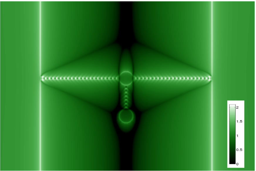
Figure 4: (Color online) Numerical calculation of the distribution of $B_{z}$ in a superconducting thin strip after an applied magnetic field was increased from zero to $H_{a}=1$. The strip contains a pattern of antidots essentially identical to the sample studied experimentally. As in MOI the image brightness represents the magnitude of $B_{z}$ as indicated in the color bar insert.

Starting with the superconductor itself, it obeys the material law, Eq. (3), which when combined with Faraday’s law, $\dot{B}_{z}=-(\nabla\times\mathbf{E})_{z}$, gives

$$\dot{B}_{z}=\nabla\cdot(\rho\nabla g)/d\,.$$ (9)

From $g(\mathbf{r},t)$ the gradient is readily calculated, and since the result allows finding $\mathbf{J}(\mathbf{r},t)$ from Eq. (4), also $\rho(\mathbf{r},t)$ is determined from Eq. (3). The task then is to find $\dot{B}_{z}$ in the non-superconducting parts, so that $\dot{g}=0$ outside the strip and $\dot{g}$ is uniform in the antidots. This cannot be calculated efficiently using direct methods due to the nonlocal relation between $\dot{B}_{z}$ and $\dot{g}$. Instead we use an iterative procedure.

For all iteration steps, $i=1...s$, $\dot{B}_{z}^{(i)}$ is fixed inside the superconductor by Eq. (9). At $i=1$, an initial guess is made for $\dot{B}_{z}^{(i)}$ outside the sample and inside the antidots, and $\dot{g}^{(i)}$ is calculated from Eq. (8). In general, this $\dot{g}^{(i)}$ does not vanish outside the strip and an improvement is obtained by

$$\dot{B}_{z}^{(i+1)}=\dot{B}_{z}^{(i)}-\mu_{0}\hat{Q}\hat{O}\dot{g}^{(i)}+C^{(i)}.$$ (10)

The projection operator $\hat{O}$ is unity outside the strip and zero everywhere else. Also, the output of the operation should be shifted to satisfy $\int d^{2}r\hat{O}g=0$. The constant $C^{(i)}$ is determined by requiring flux conservation,

$$\int d^{2}r\,[\dot{B}_{z}^{(i+1)}-\mu_{0}\dot{H}_{a}]=0.$$ (11)

Correspondingly, ${\dot{B}}_{z}^{(i+1)}$ in each of the antidots is also found by Eq. (10), but where the projection operator $\hat{O}$ now is unity in the antidot and zero everywhere else, and with $C^{(i)}$ calculated using Faraday’s law,

$$\int_{\text{antidot boundary}}\mathbf{dl}\cdot\mathbf{E}=-\int_{\text{antidot area}}d^{2}r\dot{B}_{z}.$$ (12)

Thus, at each iteration $(i)$, we run through all antidots and the outside area, and calculate $\dot{B}_{z}^{(i+1)}$. The procedure is repeated until after $i=s$ iterations $\dot{g}^{(s)}$ becomes sufficiently uniform both outside the strip and within the antidots. Then, $\dot{g}^{(s)}$ is inserted in Eq. (8), which brings us to the next time step, where the whole iterative procedure starts anew.

Several comments can be made regarding the implementation of the simulation scheme. First, the algorithm for finding $\dot{g}$ scales as $O(N\log N)$ with the total number of discrete grid points $N$. This enables simulations of large grids, say $N>10^{6}$. Second, the quality and performance is improved by a good initial value, such as $\dot{B}_{z}^{(1)}(t)=\dot{B}_{z}^{(s)}(t-\Delta t)$. Third, for small antidots there is a large perfomance gain by replacing the full operator $\hat{Q}\hat{O}$ in Eq. (10) by a local operator that only runs over the antidot. Fourth, the results can be made more robust by enforcing $\dot{J}=0$ exactly by hand after each iteration step to prevent accumulations of small unphysical currents inside the antidots with time. Finally, a robust way to satisfy Eq. (12) is to first calculate $\dot{B}_{z}$ from Eq. (9) in the antidot area using the material law as if the antidot was not there, and then choose $C^{(i)}$ so that the total flux in the antidot is the same.

At all times, the simulation scheme provides direct access to the distributions of $g$, $B_{z}$, $\mathbf{J}$, everywhere in the plane $z=0$, as well as access to $\mathbf{E}$ inside the superconductor, through Eq. (3). Note that $\mathbf{E}$ is not calculated inside the antidots or outside the sample.

V Simulation Results

Numerical simulations were carried out for a superconducting strip of width $2w$ where between the two edges there is a linear array of 40 antidots of radius $r=0.01w$ and center-to-center separation $a=4.4r$. Two larger holes of radius $0.08w$ are located on the strip center line, and with another array of 6 antidots in between. The area of calculation, $3w\times 2w$, was discretized on a $1536\times 1024$ equidistant grid. The creep exponent was $n=29$. The simulation was carried out in dimensionless units based on $J_{c}^{\prime}=J_{c}(wd\mu_{0}\dot{H}_{a}/\rho_{0}J_{c})^{1/n}$. The results can be converted to dimensional units by the transformations $J\to JJ_{c}^{\prime}$, $B_{z}\to B_{z}\mu_{0}J_{c}^{\prime}$, $t\to tJ_{c}^{\prime}/\dot{H}_{a}$ and $E\to E\rho_{0}J_{c}^{\prime}/d$.

Shown in Fig. 4 is the result of calculating the distribution of $B_{z}$ at an applied field of $H_{a}=1$ during a field ramp at the rate $\dot{H}_{a}=1$ starting from $H_{a}=0$. The magnetic flux penetrates from the edges where a critical state is established with $J\approx 1$. The antidots are clearly seen, and the flux distribution reproduces all characteristics of the magneto-optical image of Fig. 2. In particular, the simulation reproduces the high $B_{z}$ along the array of antidots, i.e., the flux guidance provided by the patterning. The excellent qualitative agreement with the experimental image on all visible scales gives strong confidence in the correctness of the simulation method.

Also the d-line₁ and d-line₂, which are clearly seen in Fig. 4, are in accordance with both the experiment and the Bean model considerations. Interestingly, the dark lines d-line₁ make an angle $\alpha=66^{\circ}$ with the strip edges, which is slightly larger than expected from the Bean model, where Eq. (1) gives $\alpha=62^{\circ}$ for $a/r=4.4$. This implies that the current flow is enhanced through the bridges between the antidots due to the use of a finite creep exponent, $n$.

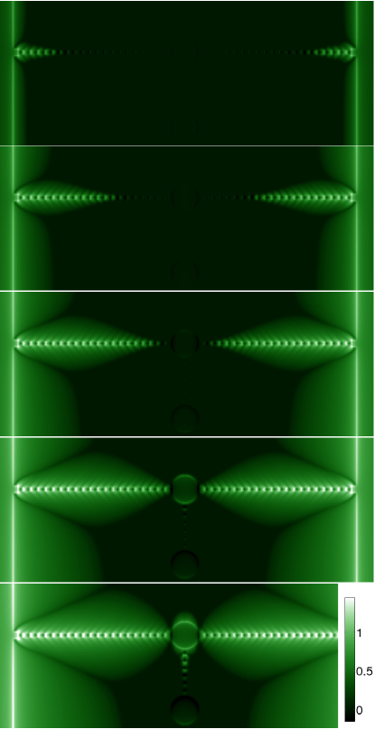
Figure 5: (Color online) Distribution of $B_{z}$ in the patterned superconducting strip at increasing applied fields of $H_{a}=0.1$(upper), $0.2$, $0.3$, 0.4 and $0.5$(lower). The inserted color bar relates the local magnitude of $B_{z}$ and the image brightness.

Figure 5 illustrates how the flux distribution evolves as the applied field is ramped up. The five panels show simulated images from $H_{a}=0.1$ to 0.5. Evidently, the flux penetration is at all stages greatly advanced along the antidot array. In fact, it extends even deeper than expected from the Bean model considerations in Fig. (1). This is due to the currents flowing in the Meissner state part of the film, where they reach the critical value when adapting to the constrictions created by the antidots.

At the field $H_{a}=0.4$, a continuous area with non-zero $B_{z}$ connects the edges and the central large hole, which first at this stage receives sizable amounts of flux. Beyond that stage, we find both experimentally and numerically that one may tune the amount of flux captured in the hole by increasing or decreasing $H_{a}$, and making the hole act as a controllable flux reservoir. Note that at $H_{a}=0.4$ the second large hole is not yet in contact with the flux front, but still faintly visible in the figure due to its perturbation of the Meissner current flow. In the final panel, $H_{a}=0.5$, flux is guided from the first large hole towards the one below following the connecting array of antidots. Here, the flux motion is parallel to the edges. The whole sequence of flux penetration patterns during increasing applied field agrees very well with the experimental results shown in Fig. 2.

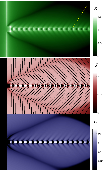
Figure 6: (Color online) Distributions of $B_{z}$, $J$ and $E$ along the left antidot array, at $H_{a}=0.4$. The $J$-map is superimposed with the current stream lines. In the $E$-map, the white spots are the bridges between the antidots, where the flux traffic is extensive. Color bars relating the image brightness and local values are shown.

Figure 7: Profiles of (a) $B_{z}$, (b) $J_{y}$, (c) $|g|$, and (d) $E_{y}$ across the antidots at $H_{a}=0.4$.

Figure 6 presents a close-up view of the antidot array at $H_{a}=0.4$. The upper panel shows the $B_{z}$, where now the fishbone structure is seen. The Bean model result, Eq. (2), predicts for the present array that the d-line₂ forms the angle $\beta=33^{\circ}$ with the edge. A dotted line at this $\beta$ is included as a guide to the eye in the figure, and it demonstrates very good agreement.

The middle panel shows the magnitude of the sheet current $J$ with the current stream lines superimposed. The main features of the current stream lines are in excellent agreement with the Bean model construction of Fig. 1, but the curving of the stream lines is less sharp due to the finite $n$. In particular, the cusps creating the d-line₂ are weak. Note that some current stream lines extend into the flux-free Meissner state region, as expected in films placed in a perpendicular magnetic field.

The lower panel shows the magnitude of the electrical field $E=|\mathbf{E}|$ in the same area. To reveal the overall field distribution the images has been plotted on a logarithmic scale, with $E$-values ranging from $10^{-3}$ to 30. Very large fields, $E>30$, were found in the bridges of superconductor connecting the antidots. Evidently, the antidot array forms a channel with large traffic of magnetic flux. At the same time, the flux motion is much reduced at the d-lines, which show up as dark also in the map of $E$, indicating suppressed traffic of magnetic flux. This is a generic feature of regions with sharply curved current streamlines.Brandt (1995)

A quantitative presentation of the profiles for $B_{z}$, $J$, $g$, and $E$ across the antidots array at $H_{a}=0.4$ is shown in Fig. 7. Clearly, all the quantities are much distorted compared to those of an unpatterned strip.Norris (1969); Brandt and Indenbom (1993); Zeldov et al. (1994) In particular, $B_{z}$ has an oscillating behaviour with minima at the inner, and maxima at the outer, edges of the antidots, where the peak values are comparable to those along the strip edge. The sheet current $J_{y}$ is zero within the antidots and is almost constant in between, with values $J\approx 1.1$. The the local magnetization $g$ has the shape of a step pyramid with flat levels across the antidots. The maximum electric field is very high, $E>50$, compared to a plain strip where $E<1$ at the edge, and it is also higher than for small indentations at a film edge.Schuster et al. (1996); Vestgården et al. (2007) The high $E$-value reflects that all magnetic flux in the diamond-shaped region has passed through channels of width comparable to the antidot diameter. Numerically, the values $E\approx 50$ and $J\approx 1.1$ are consistent, since from Eq. (3), one has $50^{1/n}\approx 1.14$ for $n=29$.

Previous works concerned with the stability of superconducting films have found that high electric field close to the edge implies that the sample is susceptible for avalanches triggered by thermomagnetic instabilities.Mints and Brandt (1996); Denisov et al. (2006) This means that a transverse array of antidots, or small defects, are likely nucleation points for the instabilities. In thin films, the consequences of the instabilities are dramatic, as they often take the form of large dendritic structures as observed in many materials.Durán et al. (1995); Bolz et al. (2003); Rudnev et al. (2005); E.-M. Choi et al. (2005)

Finally, note that the results presented in Section II were based only on current conservation, and will give a quite good description for any sample thickness provided the superconductor behaves according to the critical-state model. Thus, also the general concept of flux guidance as presented in this work should be essentially independent of thickness. On the other hand, the simulation formalism, which gives a more precise description, was derived under the assumption that the thickness is much smaller than the size of any lateral structure in the sample. Therefore, we expect that the presented simulation results will hold only as long as the antidot diameter is considerably larger than the film thickness, as was the case in the present experiments.

VI Summary

Magnetic flux guidance by linear arrays of antidots in type-II superconducting films has been considered experimentally and theoretically. Experimentally we have used MOI to show strong flux guidance in a YBCO film shaped as a long strip and patterned with antidots arranged in linear arrays. It was also shown that an antidot array along the center line can promote flux motion parallel to the strip edge. The flux penetration patterns have revealed that the antidot arrays perturb the overall flow of current considerably. In particular, we find that lines where the current flow abruptly changes direction, the d-lines, agree very well with current stream line patterns constructed from the Bean critical-state model. Further insight into the flux penetration process was achieved by numerical simulations of the electrodynamic response of the superconductor subjected to an increasing perpendicular magnetic field.

In order to perform simulations of superconducting films with complicated antidot patterns it was necessary to develop a efficient method for imposing boundary conditions, both for the sample boundaries and the antidots. The simulation of an ascending field ramp produced a flux distribution with the same qualitative and quantitative characteristics as found in the experiment. In addition, the simulations give a deeper insight into the dynamical process of flux guidance by providing information of all electrodynamic quantities at all stages of the process. It was shown that the electric field becomes very large in a thin channel connecting the antidots, in particular close to the edges. Also, maps of the electric field show that flux motion is much suppressed elsewhere near the antidots. This means that magnetic flux is guided into the film via a main route along the antidot array.