Blind topological measurement-based quantum computation

Blind quantum computation is a novel secure quantum computing protocol which enables Alice, who does not have sufficient quantum technology at her disposal, to delegate her quantum computation to Bob, who has a fully-fledged quantum computer in such a way that Bob cannot learn anything about Alice’s input, output, and algorithm. A recent proof-of-principle experiment demonstrating blind quantum computation in an optical system has raised new challenges regarding the scalability of blind quantum computation in realistic noisy conditions. Here we show that fault-tolerant blind quantum computation is possible in a topologically-protected manner using the Raussendorf-Harrington-Goyal scheme. The error threshold of our scheme is $4.3\times 10^{-3}$, which is comparable that ($7.5\times 10^{-3}$) of non-blind topological quantum computation. Since the error per gate of the order $10^{-3}$ was already achieved in some experimental systems, our result implies that secure cloud quantum computation is within reach.

In classical computing, the problem of ensuring the communication between a server and a client in secure is highly non-trivial. For example, Abadi, Feigenbaum and Killian showed that no NP-hard function can be computed with encrypted data if unconditional security is required, unless the polynomial hierarchy collapses at the third level Abadi . Even restricting the security condition to be only computational, the question of the possibility of the fully-homomorphic encryption has been a long-standing open question for 30 years Gentry , and still no practical method has been found. Unconditionally secure fully-homomorphic encryption is still an open problem.

On the other hand, in the quantum world, the situation is drastically different. Broadbent, Fitzsimons and Kashefi proposed a quantum protocol blindcluster , so-called blind quantum computation blindcluster ; Barz ; TVE ; Vedran ; blind_bell ; FK12 , which uses measurement-based quantum computation (MBQC) cluster . In their protocol, Alice has a classical computer and a quantum device that emits randomly-rotated qubits. She does not have any quantum memory. On the other hand, Bob has a fully-fledged quantum technology. Alice and Bob share a classical channel and a quantum channel. Their protocol runs as follows. First, Alice sends Bob many randomly-rotated qubits, and Bob creates a graph state by applying C$Z$ gates among these qubits. Second, Alice instructs Bob how to measure a qubit of the graph state. Third, Bob measures the qubit according to Alice’s instruction, and he returns the measurement result to Alice. They repeat this classical two-way communication (i.e., the second and third steps) until the computation is finished. It was shown blindcluster that if Bob is honest, Alice can obtain the correct answer of her desired quantum computation (correctness), and that whatever evil Bob does, he cannot learn anything about Alice’s input, output, and algorithm (blindness). Recently, this protocol has been experimentally demonstrated in an optical system Barz .

Secure delegated computation is already in the practical phase for classical computing, including smart phones, encrypted data retrieval Song , and wireless sensor networks wireless . When scalable quantum computers are realized, the need for delegated secure computation must be emphasized, since home-based quantum computers are arguably much more difficult to build than their classical counterparts. In order to implement blind quantum computation in a scalable manner, it is crucial to protect quantum computation from environmental noise. In this paper, we show that a fault-tolerant blind quantum computation is possible in a topologically protected manner. We also calculate the error threshold, $4.3\times 10^{-3}$, for erroneous preparation of the initial states, erroneous C$Z$ gates, and erroneous local measurements. This is the first time that a concrete fault-tolerant scheme is proposed for blind quantum computation, and that the error threshold is explicitly calculated. Furthermore, this threshold is not so different from that, $7.5\times 10^{-3}$, of non-blind topological quantum computation Raussendorf_PRL ; Raussendorf_NJP . In other words, blind quantum computation is possible with almost the same error threshold as that of the non-blind version. Since the error threshold of the order $10^{-3}$ was already achieved in some experimental systems ion , our result means that secure cloud quantum computation is within our reach. We further show that our protocol is also fault-tolerant against the detectable qubit loss, such as a photon loss and an escape from the qubit energy level.

I Results

I.1 Topologically-protected MBQC

The topologically-protected measurement-based quantum computation (TMBQC) Raussendorf_PRL ; Raussendorf_NJP ; topo_experiment is one of the most promising models of quantum computation. In this model, we first prepare the graph state on the three-dimensional cubic lattice $\mathcal{L}$ whose elementary cell is given in Fig. 1 (a). We call this lattice ${\mathcal{L}}$ the Raussendorf-Harrington-Goyal (RHG) lattice. We next measure each qubit of this lattice in $X$, $Z$, $T\equiv(X+Y)/\sqrt{2}$, or $Y$ basis. These four types of measurements are sufficient for the universal TMBQC as is shown in Refs. Raussendorf_PRL ; Raussendorf_NJP . (More precisely, measurements in $X$ basis and $Z$ basis can simulate the topological braidings of defects in the surface code Kitaev which can implement the fault-tolerant Clifford gates, and measurements in $T$ basis and $Y$ basis can simulate the preparations of magic states magic which can implement the non-Clifford gates. These magic states are distilled magic by topologically protected fault-tolerant Clifford gates which are simulated by $X$ and $Z$ basis measurements.) A small-size TMBQC has recently been experimentally demonstrated in an optical system topo_experiment .

I.2 Blind TMBQC

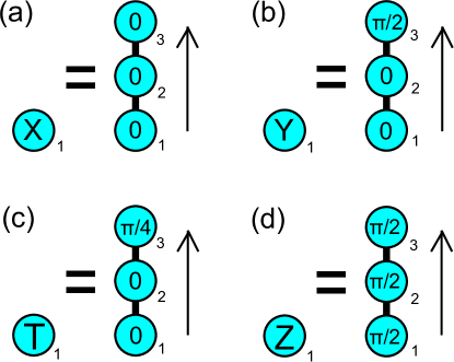
Figure 2: How the decorated lattice works. If we prepare the three-qubit cluster state and measure each qubit in the numerical order in the $\{|0\rangle\pm e^{i\phi_{j}}|1\rangle\}$ basis with $(\phi_{1},\phi_{2},\phi_{3})=(0,0,0)$, $(0,0,\pi/2)$, $(0,0,\pi/4)$, and $(\pi/2,\pi/2,\pi/2)$, we can simulate single-qubit measurements in $X$, $Y$, $T$, and $Z$ basis, respectively. Each corresponds to (a), (b), (c), and (d).

Can we use TMBQC for the blind quantum computation? Obviously, if Bob knows in which basis ($X$, $Z$, $T$, or $Y$) he is doing the measurement on each qubit, he can know Alice’s algorithm. However, if Alice can have Bob do measurements in such a way that Bob cannot know in which basis ($X$, $Z$, $T$, or $Y$) he is doing the measurement on each qubit, he cannot know Alice’s algorithm. How can Alice do that? In fact, such a blind quantum computation is possible if we consider the three-dimensional lattice ${\mathcal{L}}^{\prime}$ whose elementary cell is given in Fig. 1 (b) where two extra qubits are added to each qubit of Fig. 1 (a). We call this lattice ${\mathcal{L}}^{\prime}$ the decorated RHG lattice. The intuitive explanation of our idea is as follows: First, it was shown blindcluster that Alice can have Bob do the measurement in $\{|0\rangle\pm e^{i\phi}|1\rangle\}$ basis for any $\phi\in\{\frac{k\pi}{4}~{}|~{}k=0,1,...,7\}$ on any qubit of a graph state which Bob has in such a way that Bob cannot learn anything about $\phi$. Second, it is easy to confirm that a single-qubit measurement in $X$, $Y$, $T$, or $Z$ basis can be simulated on the linear three-qubit cluster state with only $\{|0\rangle\pm e^{i\phi}|1\rangle\}$ basis measurements (Fig. 2). By combining these two facts, we notice that if we decorate the RHG lattice as is shown in Fig. 1 (b), Bob can simulate the measurement in $X$, $Y$, $T$, and $Z$ basis only with $\{|0\rangle\pm e^{i\phi}|1\rangle\}$ basis measurements, and he cannot know which type of measurements ($X$, $Y$, $T$, or $Z$) he is simulating.

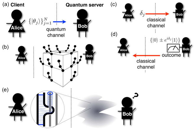
Figure 3: Topological blind protocol. (a) Alice sends Bob randomly rotated qubits. (b) Bob creates the decorated RHG lattice. (c) Alice sends Bob a classical message. (d) Bob does the measurement and returns the result to Alice. (e) Alice can hide her topological quantum computation from Bob.

More precisely, our protocol runs as follows (Fig. 3):

Step 1. Alice sends $N$ randomly-rotated single-qubit states $\{|\theta_{j}\rangle\}_{j=1}^{N}$ to Bob through the quantum channel, where

$$|\theta_{j}\rangle\equiv|0\rangle+e^{i\theta_{j}}|1\rangle,$$

and $\theta_{j}\in\{\frac{k\pi}{4}|k=0,1,...,7\}$ $(j=1,2,...,N)$ are random numbers. $N$ is the total number of qubits used in the decorated RHG lattice ${\mathcal{L}}^{\prime}$. Alice remembers all random numbers $\Theta\equiv\{\theta_{j}\}_{j=1}^{N}$, and they are kept secret to Bob.

Step 2. Now Bob has $\{|\theta_{j}\rangle\}_{j=1}^{N}$. He places $|\theta_{j}\rangle$ on the $j$th vertex of the decorated RHG lattice ${\mathcal{L}}^{\prime}$ for all $j$ ($j=1,...,N$). He then applies the C$Z$ gate on each red edge of the decorated RHG lattice ${\mathcal{L}}^{\prime}$. Let us denote thus created $N$-qubit state by $|\mathcal{C}_{\Theta}\rangle$. Since

$$|{\mathcal{C}}_{\Theta}\rangle = \Big{(}\bigotimes_{k,l}CZ_{k,l}\Big{)}\Big{(}\bigotimes_{j=1}^{N}e^{-iZ\theta_{j}/2}\Big{)}|+\rangle^{\otimes N}$$

$$= \Big{(}\bigotimes_{j=1}^{N}e^{-iZ\theta_{j}/2}\Big{)}\Big{(}\bigotimes_{k,l}CZ_{k,l}\Big{)}|+\rangle^{\otimes N},$$

$|{\mathcal{C}}_{\Theta}\rangle$ is nothing but a rotated graph state on the decorated RHG lattice ${\mathcal{L}}^{\prime}$. Here $CZ_{k,l}$ is the C$Z$ gate between $k$th and $l$th qubits.

Step 3. If Alice wants Bob to measure $j$th qubit of $|{\mathcal{C}}_{\Theta}\rangle$ in $\{|0\rangle\pm e^{i\phi_{j}}|1\rangle\}$ basis, she calculates

$$\delta_{j}\equiv\phi^{\prime}_{j}+\theta_{j}+r_{j}\pi~{}~{}(\mbox{mod}~{}2\pi)$$

on her classical computer. Here, $r_{j}\in\{0,1\}$ is a random number, $\phi^{\prime}_{j}\equiv(-1)^{s_{j}^{X}}\phi_{j}+\pi^{s_{j}^{Z}}$ (mod $2\pi$), and $s_{j}^{X},s_{j}^{Z}\in\{0,1\}$ are determined by the previous measurement results (this is the usual feed-forwarding in the one-way model cluster ). Then Alice sends $\delta_{j}$ to Bob through the classical channel.

Step 4. Bob measures $j$th qubit in the $\{|0\rangle\pm e^{i\delta_{j}}|1\rangle\}$ basis, and returns the result of the measurement to Alice through the classical channel.

Step 5. They repeat steps 3 and 4 with increasing $j$ until they finish the computation. Note that Alice does the classical processing for the error correction by using Bob’s measurement results.

I.3 Correctness

Let us show that this protocol is correct. In other words, Alice and Bob can simulate the original TMBQC Raussendorf_PRL ; Raussendorf_NJP on the decorated RHG lattice ${\mathcal{L}}^{\prime}$ with only $\{|0\rangle\pm e^{i\phi}|1\rangle\}$ basis measurements if Bob is honest. Let us consider three qubits labeled with 1, 2, and 3, in Fig. 1 (b). Let us assume that Bob measures these three qubits in the numerical order (i.e., from the bottom one to the top one) in the

$$\{|0\rangle\pm e^{i\delta_{j}}|1\rangle\}=\Big{\{}e^{-i\theta_{j}Z/2}Z^{s^{Z}_{j}}X^{s^{X}_{j}}\big{(}|0\rangle\pm e^{i\phi_{j}}|1\rangle\big{)}\Big{\}}$$

basis ($j=1,2,3$) with $(\phi_{1},\phi_{2},\phi_{3})=(0,0,0)$. By a straightforward calculation, it is easy to show that such a sequence of measurements on the three qubits is equivalent to the measurement in $X$ basis on the qubit labeled with 1 in Fig. 1 (a) (also Fig. 2 (a)). (Note that $\theta_{j}$ in Bob’s measurement basis is canceled since $j$th qubit is pre-rotated by $\theta_{j}$ by Alice. Furthermore, $r_{j}\pi$ causes just the flip of the measurement result. Therefore, Bob effectively does $\{|0\rangle\pm e^{i\phi_{j}}|1\rangle\}$ basis measurement although he is doing $\{|0\rangle\pm e^{i\delta_{j}}|1\rangle\}$ basis measurement.) In other words, our lattice ${\mathcal{L}}^{\prime}$ can simulate $X$ basis measurements on ${\mathcal{L}}$. In a similar way, if Bob does measurements on the three qubits labeled with 1, 2, and 3 in Fig. 1 (b) in other angles, $(\phi_{1},\phi_{2},\phi_{3})=(0,0,\pi/2)$, $(0,0,\pi/4)$, and $(\pi/2,\pi/2,\pi/2)$, they are equivalent to the $Y$, $T$, and $Z$ basis measurements on the qubit labeled with 1 in Fig. 1 (a), respectively (Fig. 2 (b), (c), and (d)). In this way, our lattice ${\mathcal{L}}^{\prime}$ can simulate $X$, $Z$, $T$, and $Y$ basis measurements on ${\mathcal{L}}$. In short, we have shown that $|{\mathcal{C}}_{\Theta}\rangle$ on the decorated RHG lattice ${\mathcal{L}}^{\prime}$ can simulate the original TMBQC Raussendorf_PRL ; Raussendorf_NJP on the RHG lattice ${\mathcal{L}}$ solely with $\{|0\rangle\pm e^{i\phi}|1\rangle\}$ basis measurements.

I.4 Blindness

How about the blindness? In our protocol, what Alice sends to Bob are randomly rotated single-qubit states $\{|\theta_{j}\rangle\}_{j=1}^{N}$ and measurement angles $\{\delta_{j}\}_{j=1}^{N}$. Without loss of generality, we can assume that the preparation of the input is included in the algorithm. Therefore, what Alice wants to hide are the algorithm and the output. We can show that the conditional probability distribution of Alice’s computational angles, given all the classical information Bob can obtain during the protocol, and given the measurement results of any POVMs which Bob may perform on his system at any stage of the protocol, is equal to the a priori probability distribution of Alice’s computational angles. We can also show that the final classical output is one-time padded to Bob. (For a proof, see Methods.)

I.5 Threshold

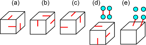
Figure 4: The stepwise creation of the resource state. $|\mathcal{C}_{\Theta}\rangle$ is created from (a) to (e).

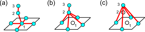
Figure 5: The measuring pattern. Three qubits are measured in the numerical order from (a) to (c).

Finally, let us calculate the fault-tolerant threshold. As in Refs. Raussendorf_PRL ; Raussendorf_NJP , we assume that errors occur during the preparation of initial states $\{|\theta_{j}\rangle\}_{j=1}^{N}$, the applications of C$Z$ gates, and the local measurements. The erroneous preparation of an initial state is modeled by the perfect preparation followed by the partially depolarizing noise with the probability $p_{P}$: $(1-p_{P})[I]+\frac{p_{P}}{3}([X]+[Y]+[Z])$, where $[\bullet]$ indicates the super operator. The erroneous local measurement is modeled by the perfect local measurement preceded by the partially depolarizing noise with the probability $p_{M}$. The erroneous C$Z$ gate is modeled by the perfect C$Z$ gate followed by the two-qubit partially depolarizing noise with the probability $p_{2}$: $(1-p_{2})[I\otimes I]+\frac{p_{2}}{15}([I\otimes X]+...+[Z\otimes Z])$. Because of the rotational symmetry of the depolarizing noise, we can replace $[A]$ with $[e^{-i\theta_{j}Z/2}Ae^{i\theta_{j}Z/2}]$ when it acts on the $j$th qubit, and $[A\otimes B]$ with $[(e^{-i\theta_{j}Z/2}Ae^{i\theta_{j}Z/2})\otimes(e^{-i\theta_{k}Z/2}Be^{i\theta_{k}Z/2})]$ when it acts on the $j$th and $k$th qubits. Here, $A,B=I,X,Y$ or, $Z$. These replacements just correspond to the rotation of the local reference frame of each qubit. Then, if the measurement basis on the $j$th qubit ($j=1,...,N$) is rotated by $e^{-i\theta_{j}Z/2}$, the factor $\bigotimes_{j=1}^{N}e^{-i\theta_{j}Z/2}$ is canceled. Therefore, when we calculate the fault-tolerant threshold of our protocol, we can assume that all $\theta_{j}=0$ without loss of generality. As in Ref. Raussendorf_Ann , we assume that $|\mathcal{C}_{\Theta}\rangle$ is created in the stepwise manner (Fig. 4). In our case, however, the additional fifth step is introduced as is shown in Fig. 4 (e). First, let us calculate the single-qubit $Z$ error probability $\lambda_{j}$ $(j=1,2,3)$ on each of the three qubits labeled with $1,2,3$ in Fig. 1 (b) after creating $|\mathcal{C}_{\Theta}\rangle$. By a straightforward calculation, we obtain $\lambda_{1}=32p_{2}/15+8p_{2}/15+2p_{P}/3$, $\lambda_{2}=16p_{2}/15+2p_{P}/3$, and $\lambda_{3}=8p_{2}/15+2p_{P}/3$ up to the first order of $p_{P}$ and $p_{2}$. Once an erroneous $|\mathcal{C}_{\Theta}\rangle$ is created, we start local measurements. As is shown in Fig. 5, the three qubits are sequentially measured in numerical order. Such a sequential measurement propagates all pre-existing errors on qubits labeled with 1 and 2 to the qubit labeled with 3. By a straightforward calculation, the accumulated error probability on the qubit labeled with 3 by such a propagation is $\lambda_{total}\equiv\lambda_{1}+\lambda_{3}+2\times 2p_{M}/3$ for $(\phi_{1},\phi_{2},\phi_{3})=(0,0,0)$. (We have only to consider the measurement pattern which corresponds to the effective $X$ measurement on the qubit labeled with 1 in Fig. 1 (a), because we are now interested in the topological error-correction of the bulk qubits.) The value $\lambda_{total}$ corresponds to the quantity $q_{1}$, which was studied in Ref. Raussendorf_Ann , of the qubit labeled with 1 in Fig. 1 (a). The correlated two-qubit error probability Raussendorf_Ann $q_{2}=4p_{2}/15+O(p_{2}^{2})$ in our protocol is the same as that in Ref. Raussendorf_Ann . If we assume $p_{P}=p_{M}=p_{2}=p$, we obtain the bulk topological error threshold as $p=4.3\times 10^{-3}$ from Fig. 10 of Ref. Raussendorf_Ann where the threshold curve of $(q_{1},q_{2})$ is numerically calculated by using the minimum-weight-perfect-matching algorithm.

The primal defects are created by measuring the edge qubits inside the defect region in the $Z$ basis. At the boundary of the defect region (surface of the defects), these measurements introduce additional $Z$ errors on the face qubits (i.e., dual qubits), which has an effect of decreasing the threshold value. At the same time, the existence of the defects changes the boundary condition of the bulk region; at the surface of the primal defects, the dual lattice has a smooth boundary. Thus, there is excess syndrome available at the defect surface, which has an effect of increasing the threshold value. In Ref. Raussendorf_Ann , they have performed numerical simulation for lattices of size $L\times L\times 2L$, where half of the lattice belongs to the bulk region $V$ and the other half to the defect region $D$. In their calculations, the error probability of the dual qubits of the surface of the defect is doubled to investigate the surface effect. Their numerical result indicates that while the surface effect due to the smooth boundary (i.e., increasing the threshold value) is noticeable, the intersection point of fidelity curves is slowly converging to the threshold value of the bulk region in the increasing number of the lattice size. This indicates that the $Z$ basis measurements for the defect creations do not lower the threshold for TMBQC. In the present case, the error probability of $Z$ basis measurement is increased by $\lambda_{Z}=2(2p_{M}/3)+2(2p_{P}/3)+p_{2}$ due to the additional qubits for the blind $Z$ basis measurement. However, when $p_{M}=p_{P}=p_{2}=4.3\times 10^{-3}$, the error probability $\lambda_{Z}=1.6\times 10^{-2}$ is still smaller than the situation that has been considered in Ref. Raussendorf_Ann . Thus the defect creations do not lower the threshold in the blind setup again, and hence the threshold value is determined by that for the bulk region.

Topological error correction breaks down near the singular qubits, and it results in an effective error on the singular qubits Raussendorf_PRL ; Raussendorf_NJP . This effective error is local because singular qubits are well separated from each other. Magic state distillation magic can tolerate a rather large amount of noise, and therefore the overall threshold is determined by that for the bulk topological region Raussendorf_PRL ; Raussendorf_NJP . In fact, the recursion relations of the distillations of $Y$ and $(X+Y)/\sqrt{2}\equiv T$ basis states are given by $\epsilon^{Y}_{l+1}=7(\epsilon^{Y}_{l})^{3}+\epsilon_{top}^{Y}$ and $\epsilon^{T}_{l+1}=35(\epsilon^{T}_{l})^{3}+\epsilon_{top}^{T}$, where $\epsilon_{top}^{Y}$ and $\epsilon_{top}^{T}$ indicate the probability of errors introduced by the Clifford gates for the magic state distillation Raussendorf_NJP . In order to optimize their overheads, the scale factor and defect thickness at each distillation level are chosen so that $\epsilon_{l}^{Y,T}$ and $\epsilon_{top}^{Y,T}$ are balanced. Since $\epsilon_{top}^{Y}$ and $\epsilon_{top}^{T}$ can be reduced rapidly by increasing the scale factor and the thickness of the defect, the threshold values for the magic state distillation can be determined as $\epsilon^{Y}=0.38$ and $\epsilon^{T}=0.17$ for $Y$- and $T$-state distillations, respectively. In the present decorated case, the error probability of the injected magic state is at most $\epsilon=4p_{2}+2p_{2}+3(2p_{M}/3)+3(2p_{P}/3)$, where the first, second, third, and forth terms indicate four C$Z$ gates for generating RHG lattice, two C$Z$ gates for the decoration, three measurements, and three state preparations. With $p_{M}=p_{P}=p_{2}=4.3\times 10^{-3}$, $\epsilon=10p_{2}=0.043$ which is sufficiently smaller than the threshold values for the magic state distillations.

In the above arguments, we have assumed $p_{P}=p_{M}=p_{2}$ for simplicity. However, $p_{P}$ might be much larger than $p_{M}$ and $p_{2}$, since Alice’s quantum technology is assumed to be much weaker than that of Bob, and the randomly-rotated qubits are sent from Alice to Bob through a probably noisy quantum channel. (In addition, Alice cannot distill her qubits, since she cannot use any two-qubit gate.) Hence let us consider another representative scenario, $p_{P}=10p$, $p_{M}=p_{2}=p$. Interestingly, the direct calculation shows that the error threshold is $p=1.6\times 10^{-3}$ (i.e., still of the order of $10^{-3}$). This suggests the nice robustness on Alice’s side in the topological fault-tolerant protocol. (Note that this result is reasonable because the preparation error behaves as an independent error, and independent errors are known to be easy to correct. In fact, if there is no correlated error, TMBQC can tolerates the independent error up to 2.9%.)

II Discussion

In addition to the probabilistic depolarizing noise, which we have considered, there are many possibilities of errors. For example, quantum computation can suffer from the detectable qubit loss, such as photon loss, atoms or ions escaping from traps, or, more generally, the leakage of a qubit out of the computational basis in a multilevel system. In Ref. Barrett_loss , the threshold of the TMBQC for the qubit loss was studied. Here let us briefly explain that we can obtain a similar threshold for the qubit loss in our blind protocol. As in Ref. Barrett_loss , let us assume that losses are independent and identically distributed events with the probability $p_{loss}$. If one of the three qubits labeled with 1, 2, and 3 in Fig. 1 (b) is lost, then we just consider the entire three-qubit chain is lost. Then, we can use the result of Ref. Barrett_loss , and our threshold for the qubit loss is obtained by replacing their $p_{loss}$ with $3p_{loss}$. Note that if we also use the post-selected scheme of Ref. Barrett_loss , then the overhead is $\simeq(1-3p_{loss})^{d^{3}}$, which is still independent of the size of the algorithm and hence ensuring scalability. Another possible error, the non-determinism of C$Z$ gates, was considered in Refs. Fujii ; Li for TMBQC. For example, in Ref. Fujii , the three-dimensional resource state is created by fusing the “puffer ball” states. If the one-dimensional chain of two qubits is added to the root qubit of each puffer ball state, $|\mathcal{C}_{\Theta}\rangle$ can be created by a similar fusion strategy, and the threshold can also be calculated in a similar way.

Although the simulation of fault-tolerant quantum circuits in the blind MBQC on the brickwork state was mentioned in Ref. blindcluster , it is only the existence proof. Neither a concrete scheme nor an explicit calculation of the threshold was given. Furthermore, on the two-dimensional brickwork state, we should use the fault-tolerant scheme of the one-dimensional nearest-neighbour circuit model architecture. For the circuit model, the threshold of this scheme is of the order of $10^{-5}$ Stephens1 ; Stephens2 . If we implement this scheme on MBQC, the threshold should be $\sim 10^{-6}$ due to the extra qubits Dawson1 ; Dawson2 . As is mentioned in Ref. blindcluster , the threshold should be increased if the three-dimensional brickwork state is considered. However, the explicit calculation of the threshold for the scheme of Ref. Gottesman is not known and should be smaller than that of TMBQC.

In the protocol, Alice performs the decoding operation (error correction) by using the classical data from Bob Raussendorf_PRL ; Raussendorf_NJP . We have calculated the threshold value for the present blind protocol by following the result in Ref. Raussendorf_Ann , where the minimum-weight-perfect-matching algorithm is used for the decoding problem. Although the minimum-weight-perfect-matching is an efficient algorithm in the sense that it scales polynomially, it might cost large classical computational resources when the lattice size is large. However, more efficient classical algorithms for the decoding problem have also been developed Fowler3 ; Poulin1 ; Poulin2 , one of which Fowler3 achieves the decoding of the lattice of 4 million qubits within a few seconds by using a today’s typical classical computer, while the resultant threshold $0.9\%$ is higher than that $0.75\%$ in Ref. Raussendorf_Ann . In this sense, Alice’s classical processing does not present any problem here.

III Methods

III.1 Definition of the blindness

Here we show the blindness of our protocol. Intuitively, a protocol is blind if Bob, given all the classical and quantum information during the protocol, cannot learn anything about Alice’s computational angles, input and output blindcluster ; TVE ; Vedran . A formal definition we adopt here is as follows. (See also Refs. blindcluster ; TVE ; Vedran .)

A protocol is blind if: (B1) the conditional probability distribution of Alice’s computational angles, given all the classical information Bob can obtain during the protocol, and given the measurement results of any POVMs which Bob may perform on his system at any stage of the protocol, is equal to the a priori probability distribution of Alice’s computational angles; and (B2) the final classical output is one-time padded to Bob.

III.2 Our protocol satisfies B1

Let us define $\Delta\equiv(\Delta_{1},...,\Delta_{N})$, $\Phi\equiv(\Phi_{1},...,\Phi_{N})$, $\Theta\equiv(\Theta_{1},...,\Theta_{N})$, $R\equiv(R_{1},...,R_{N})$, where $\Delta_{j},\Theta_{j},\Phi_{j}\in{\mathcal{A}}\equiv\{\frac{k\pi}{4}|k=0,1,...,7\}$ and $R_{j}\in\{0,1\}$ are random variables, corresponding to the angles sent by Alice to Bob, random prerotations, Alice’s secret computational angles, and the hidden binary parameters, respectively. From the construction of the protocol, the relation $\Delta_{j}=\Phi_{j}+\Theta_{j}+R_{j}\pi$ $(\mbox{mod}~{}2\pi)$ is satisfied. Let $\{\Pi_{j}\}_{j=1}^{m}$ be a POVM which Bob may perform on his $\{|\theta_{j}\rangle\}_{j=1}^{N}$. Let $O\in\{1,...,m\}$ be the random variable corresponding to the result of the POVM. Bob’s knowledge about Alice’s computational angles is given by the conditional probability distribution of $\Phi=(\phi_{1},...,\phi_{N})$ given $O=j$ and $\Delta=(\delta_{1},...,\delta_{N})$: $P(\Phi=(\phi_{1},...,\phi_{N})|O=j,\Delta=(\delta_{1},...,\delta_{N}))$.

From Bayes’ theorem, we have

$$P\Big{(}\Phi=(\phi_{1},...,\phi_{N})\Big{|}O=j,\Delta=(\delta_{1},...,\delta_{N})\Big{)}$$

$$= \frac{P\Big{(}O=j\Big{|}\Phi=(\phi_{1},...,\phi_{N}),\Delta=(\delta_{1},...,\delta_{N})\Big{)}P\Big{(}\Phi=(\phi_{1},...,\phi_{N}),\Delta=(\delta_{1},...,\delta_{N})\Big{)}}{P\Big{(}O=j,\Delta=(\delta_{1},...,\delta_{N})\Big{)}}$$

$$= \frac{P\Big{(}O=j\Big{|}\Phi=(\phi_{1},...,\phi_{N}),\Delta=(\delta_{1},...,\delta_{N})\Big{)}P\Big{(}\Phi=(\phi_{1},...,\phi_{N})\Big{)}P\Big{(}\Delta=(\delta_{1},...,\delta_{N})\Big{)}}{P\Big{(}O=j\Big{|}\Delta=(\delta_{1},...,\delta_{N})\Big{)}P\Big{(}\Delta=(\delta_{1},...,\delta_{N})\Big{)}}$$

$$= P\Big{(}\Phi=(\phi_{1},...,\phi_{N})\Big{)}\frac{\mbox{Tr}\Big{[}\Pi_{j}\bigotimes_{i=1}^{N}\frac{1}{2}\sum_{r_{i}=0}^{1}|\delta_{i}-\phi_{i}-r_{i}\pi\rangle\langle\delta_{i}-\phi_{i}-r_{i}\pi|\Big{]}}{\mbox{Tr}\Big{[}\Pi_{j}\bigotimes_{i=1}^{N}\frac{1}{8}\frac{1}{2}\sum_{\phi_{i}\in{\mathcal{A}}}\sum_{r_{i}=0}^{1}|\delta_{i}-\phi_{i}-r_{i}\pi\rangle\langle\delta_{i}-\phi_{i}-r_{i}\pi|\Big{]}}$$

$$= P\Big{(}\Phi=(\phi_{1},...,\phi_{N})\Big{)}.$$

III.3 Our protocol satisfies B2

It is easy to confirm that when Bob measures the qubit labeled with 3 in Fig. 1 (b), the state is one-time padded with $Z^{s_{1}}X^{s_{2}}$, where $s_{1}$ ($s_{2}$) is the measurement result of the qubit labeled with 1 (2) in Fig. 1 (b). The values of $s_{1}$ and $s_{2}$ are unknown to Bob, since $\{r_{j}\}_{j=1}^{N}$ are unknown to Bob. We can show that $\{r_{j}\}_{j=1}^{N}$ are unknown to Bob as follows.

$$P\Big{(}R=(r_{1},...,r_{N})\Big{|}O=j,\Delta=(\delta_{1},...,\delta_{N})\Big{)}$$

$$= \frac{P\Big{(}O=j\Big{|}R=(r_{1},...,r_{N}),\Delta=(\delta_{1},...,\delta_{N})\Big{)}P\Big{(}R=(r_{1},...,r_{N}),\Delta=(\delta_{1},...,\delta_{N})\Big{)}}{P\Big{(}O=j,\Delta=(\delta_{1},...,\delta_{N})\Big{)}}$$

$$= \frac{P\Big{(}O=j\Big{|}R=(r_{1},...,r_{N}),\Delta=(\delta_{1},...,\delta_{N})\Big{)}P\Big{(}R=(r_{1},...,r_{N})\Big{)}P\Big{(}\Delta=(\delta_{1},...,\delta_{N})\Big{)}}{P\Big{(}O=j\Big{|}\Delta=(\delta_{1},...,\delta_{N})\Big{)}P\Big{(}\Delta=(\delta_{1},...,\delta_{N})\Big{)}}$$

$$= P\Big{(}R=(r_{1},...,r_{N})\Big{)}\frac{\mbox{Tr}\Big{[}\Pi_{j}\bigotimes_{i=1}^{N}\frac{1}{8}\sum_{\phi_{i}\in{\mathcal{A}}}|\delta_{i}-\phi_{i}-r_{i}\pi\rangle\langle\delta_{i}-\phi_{i}-r_{i}\pi|\Big{]}}{\mbox{Tr}\Big{[}\Pi_{j}\bigotimes_{i=1}^{N}\frac{1}{8}\frac{1}{2}\sum_{\phi_{i}\in{\mathcal{A}}}\sum_{r_{i}=0}^{1}|\delta_{i}-\phi_{i}-r_{i}\pi\rangle\langle\delta_{i}-\phi_{i}-r_{i}\pi|\Big{]}}$$

$$= P\Big{(}R=(r_{1},...,r_{N})\Big{)}$$

$$= \frac{1}{2^{N}}.$$

Acknowledgement We acknowledge supports from JSPS, ANR (StatQuant, JC07 07205763), and MEXT(Grant-in-Aid for Scientific Research on Innovative Areas 20104003).

Author contributions Both authors contributed equally to this work.

Author information Correspondence and requests for materials should be addressed to T.M. (morimae@gmail.com). The authors declare no competing financial interests.

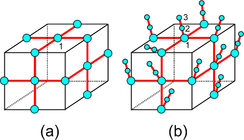
Figure 1: Elementary cells. (a): The elementary cell of the RHG lattice $\mathcal{L}$. (b): The elementary cell of the decorated RHG lattice ${\mathcal{L}}^{\prime}$.

References

-
(1)
Abadi, M., Feigenbaum, J.,
&Kilian, J. On hiding information from an oracle, J. of Comput. and System Sci. 39, 21-50 (1989). - (2) Gentry, C. Fully homomorphic encryption using ideal lattices, in Proc. of the 41st annual ACM Sympo. on Theor. of Comput. 169-178 (2009).
-
(3)
Broadbent, A., Fitzsimons, J.,
&Kashefi, E. Universal blind quantum computation, in Proc. of the 50th Annual IEEE Sympo. on Found. of Comput. Sci. (FOCS 2009) 517-527 (2009). -
(4)
Barz, S., Kashefi, E., Broadbent, A., Fitzsimons, J.,
Zeilinger, A.,
&Walther, P. Experimental demonstration of blind quantum computing, Science 335, 303-308 (2012). -
(5)
Morimae, T., Dunjko, V.,
&Kashefi, E. Ground state blind quantum computation on AKLT state, Preprint at arXiv:1009.3486 (2010). -
(6)
Dunjko, V., Kashefi, E.,
&Leverrier, A. Universal blind quantum computing with coherent states, Phys. Rev. Lett. 108, 200502 (2012). -
(7)
Morimae, T.
&Fujii, K. Blind quantum computation for Alice who does only measurements, Preprint at arXiv:1201.3966 (2012). -
(8)
Fitzsimons, J.
&Kashefi, E. Unconditionally verifiable blind computation, Preprint at arXiv:1203.5217 (2012). -
(9)
Raussendorf R.
&Briegel, H. J. A one-way quantum computer, Phys. Rev. Lett. 86, 5188 (2001). -
(10)
Song, D., Wagner, D.,
&Perrig, A. Practical Techniques for Searches on Encrypted Data, in IEEE Sympo. on Research in Security and Privacy (2000). -
(11)
Castelluccia, C., Mykletun, E.,
&Tsudik, G. Efficient aggregation of encrypted data in wireless sensor networks, in ACM/IEEE Mobile and Ubiquitous Systems: Networking and Services (Mobiquitous’05), pp.109-117 (2005). -
(12)
Raussendorf, R.
&Harrington, J. Fault-tolerant quantum computation with high threshold in two dimensions, Phys. Rev. Lett. 98, 190504 (2007). -
(13)
Raussendorf, R., Harrington, J.,
&Goyal, K. Topological fault-tolerance in cluster state quantum computation, New J. of Phys. 9, 199 (2007). -
(14)
Benhelm, J., Kirchmair, G., Roos, C. F.,
&Blatt, R. Towards fault-tolerant quantum computing with trapped ions, Nature Phys. 4, 463-466 (2008). -
(15)
Yao, X. C., Wang, T. X., Chen, H. Z., Gao, W. B., Fowler, A. G.,
Raussendorf, R., Chen, Z. B., Liu, N. L., Lu, C. Y., Deng, Y. J.,
Chen, Y. A.,
&Pan, J. W. Experimental demonstration of topological error correction, Nature 482, 489-494 (2012). - (16) Kitaev, A. Fault-tolerant quantum computation by anyons, Ann. Phys. 303, 2-30 (2003).
-
(17)
Bravyi, S.
&Kitaev, A. Universal quantum computation with ideal Clifford gates and noisy ancillas, Phys. Rev. A 71, 022316 (2005). -
(18)
Raussendorf, R., Harrington, J.,
&Goyal, K. A fault-tolerant one-way quantum computer, Ann. Phys. 321, 2242-2270 (2006). -
(19)
Barrett, S. D.
&Stace, T. M. Fault tolerant quantum computation with very high threshold for loss errors, Phys. Rev. Lett. 105, 200502 (2010). -
(20)
Fujii, K.
&Tokunaga, Y. Fault-tolerant topological one-way quantum computation with probabilistic two-qubit gates, Phys. Rev. Lett. 105, 250503 (2010). -
(21)
Li, Y., Barrett, S. D., Stace, T. M.,
&Benjamin, S. C. Fault tolerant quantum computation with nondeterministic gates, Phys. Rev. Lett. 105, 250502 (2010). -
(22)
Stephens, A. M., Fowler, A. G.,
&Hollenberg, L. C. L. Universal fault tolerant quantum computation on bilinear nearest neighbor arrays, Quant. Inf. Comput. 8, 330-344 (2008). -
(23)
Stephens, A. M.
&Evans, Z. W. E. Accuracy threshold for concatenated error detection in one dimension, Phys. Rev. A 80, 022313 (2009). -
(24)
Dawson, C. M., Haselgrove, H. L.,
&Nielsen, M. A. Noise thresholds for optical cluster-state quantum computation, Phys. Rev. A 73, 052306 (2006). -
(25)
Dawson, C. M., Haselgrove, H. L.,
&Nielsen, M. A. Noise thresholds for optical quantum computers, Phys. Rev. Lett. 96, 020501 (2006). - (26) Gottesman, D. Fault-tolerant quantum computation with local gates, J. Mod. Opt. 47, 333-345 (2000).
-
(27)
Fowler, A. G., Whiteside, A. C.,
&Hollenberg, L. C. L. Towards practical classical processing for the surface code, Phys. Rev. Lett. 108, 180501 (2012). -
(28)
Duclos-Cianci, G.,
&Poulin, D. Fast decoders for topological quantum codes, Phys. Rev. Lett. 104, 050504 (2010). -
(29)
Duclos-Cianci, G.,
&Poulin, D. A renormalization group decoding algorithm for topological quantum codes, Preprint at arXiv:1006.1362 (2010).