Complete experimental characterization of a superconducting multiphoton nanodetector

Abstract

We present a complete method to characterize multiphoton detectors with a small overall detection efficiency. We do this by separating the nonlinear action of the multiphoton detection event from linear losses in the detector. Such a characterization is a necessary step for quantum information protocols with single and multiphoton detectors and can provide quantitative information to understand the underlying physics of a given detector. This characterization is applied to a superconducting multiphoton nanodetector, consisting of an NbN nanowire with a bowtie-shaped subwavelength constriction. Depending on the bias current, this detector has regimes with single and multiphoton sensitivity. We present the first full experimental characterization of such a detector.

1) Leiden University, Niels Bohrweg 2, 2333 CA Leiden, the Netherlands
2) COBRA Research Institute, Eindhoven University of Technology, P.O. Box 513, 5600 MB Eindhoven, the Netherlands
3) Istituto di Fotonica e Nanotecnologie (IFN), CNR, via Cineto Romano 42, 00156 Roma, Italy

renema@physics.leidenuniv.nl

(270.5290) Photon Statistics (040.0400) Detectors (270.4180) Multi-photon Processes

1 Introduction

Multiphoton detection is a vital tool for optical quantum computing [1]. Such multiphoton detection can take many forms, two important examples of which are photon-number resolved detection, where the detector is able to distinguish precisely the number of photons, and threshold detection, where the detector is merely able to distinguish between the cases ’N photons or more’ and ’fewer than N photons’ [2].

The common factor in all multiphoton detectors is that they are based on a nonlinear mechanism such that the response of the detector depends in some nontrivial way on the number of photons impinging on the detector. There is typically also a finite probability that a photon impinging on the detector does not participate in the detection process at all. Such losses can be modeled as attenuation of the input state impinging on an ideal (i.e. 100% efficient) detector [2].

A well-established tool to characterize any quantum detector is detector tomography, for which the mathematical framework is that of Positive Operator Valued Measures (POVM) [2, 3, 4]. In this characterization technique, the goal is to find the probability that the detector clicks, given that N photons are incident on the detector. These probabilities can be determined by illuminating the detector with a set of coherent states, and measuring the probability that the detector clicks as function of the input power. The power of detector tomography is that it allows us to characterize the detector using only coherent states as a probe. To do this, it takes into account the distribution of photon numbers in a coherent state and gives the probability of the detector responding to N photons.

Without introducting further assumptions, detector tomography is not immediately applicable in the situation where there is a large and unknown loss component in the detector. In this regime, the outcome would be heavily influenced by the probabilities dictated by the linear losses. To characterize the mulitphoton behaviour of the nonlinear detection mechanism, the range of test states would have to be large (of the order $\eta_{sde}^{-1}$, where $\eta_{sde}$ is the system detection efficiency) which would result in an overwhelming number of free parameters leading to a strongly overdetermined system.

In this work, we present a method to separate the nonlinear detection mechanism from the linear loss. We apply this method to the case of an NbN nanodetector, where we obtain the first full experimental characterization of such a detector.

This characterization gives the complete statistics of the response of the detector to any incoming state, which is of interest when a detector is used in a quantum communication or quantum information experiment. In addition, since this characterization is model-independent, it can be used to investigate the physics of the detection mechanism. This latter application is especially important in detectors where the detection mechanism is not fully understood, as is the case for an NbN nanodetector [5].

2 NbN Nanodetectors

NbN Nanodetectors consist of a bow-tie shaped constriction in an NbN nanowire [6]. The width of this constriction can be as small as 50 nm. This detector functions on the same detection principle as the well-known NbN meanders [7]. A detection event happens when one or more photons induce a break in the superconductivity and cause the formation of a resistive bridge across the detector [5], causing a voltage pulse which is detected by the readout electronics. In the nanodetector, since the bias current density is only high around the constriction, this detector has subwavelength resolution [6]. Furthermore, it is possible to lower the bias current to such a value that multiple photons are required to provide a perturbation that is strong enough to break the superconductivity. Operation in this regime results in a subwavelength multiphoton detector. Such a detector may allow for subwavelength mapping of optical fields and high-resolution near-field multiphoton microscopy.

The operation of the NbN nanodetector differs from that of an ideal N-photon threshold detector, as was already observed in the first paper announcing the construction of such a device [6]. In order for these detectors to be used in e.g. subwavelength mapping of N-photon optical fields, it is vital that their response to different photon numbers is well understood [8].

A complete characterization of the detector may also be of fundamental interest for the study of the more well-known NbN nanowire meander detectors [7]. Due to the well-localized sensitive area of the detector, the multiphoton regime is more apparent and more easily understood in a nanodetector as compared to an NbN meander, where two impinging photons are most likely absorbed in different areas of the detector. Furthermore, it has been suggested that unintended constrictions form an important limitation on the performance of an NbN meander [9]. In these respects, NbN nanodetectors may serve as models for the response of NbN meanders.

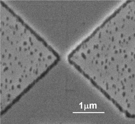
Figure 1: SEM image of the NbN nanodetector. The smooth gray area is the NbN, with the constriction in the middle. From this image, the width of the constriction was estimated to be 150 nm.

3 Experimental setup

The NbN nanodetector used in this experiment was manufactured on an NbN film deposited by DC magnetron sputtering on a GaAs substrate [10]. A nanodetector was patterned out of the NbN film by means of Electron Beam Lithography (EBL) and Reactive Ion Etching technique (RIE). The width of the constriction was estimated to be 150 nm (see figure 1). The detector was cooled in a VeriCold cryocooler with a final Joule-Thompson stage to 1.17 K. The detector critical current was measured to be 29 $\mu$A.

We illuminate the sample with a Fianium supercontinuum laser with a repetition rate of 20 MHz and a pulse width of 6 ps, which was filtered to have a center wavelength of 1500 nm, with a spectral width of 10 nm. The detector was illuminated through a single-mode lensed fiber producing a nominal spot size of 3 $\mu$m at 1500 nm. The readout electronics consist of a bias-tee (Minicircuits ZNBT-60-1W+), an amplifier chain and a pulse counter.

Each experiment consists of a large series (¿20) of experimental runs, each at constant light power, where the current through the detector is swept by means of voltage biassing, resulting in steps of 0.2 $\mu$A, up to the critical current. Power stability during each run was monitored by a power meter which receives a pick-off beam from a beam splitter in the fiber leading to the experiment. Finally, the 2-dimensional set of count rates $C(I_{b},N)$ is rearranged and normalized by the repetition rate of the laser to yield the detection probability per pulse $R(N)$ at fixed bias current $I_{b}$.

For each experiment, the power was varied so as to obtain the complete detector response curve from detection probability $R=10^{-6}$ to $R=1$. This required varying the input power over 5 orders of magnitude, typically from 20 pW to 5 $\mu$W input power into the cryostat. At a repetition rate of 20 MHz the largest input power corresponds to $N=2*10^{6}$ incident photons per pulse. Since the detection efficiency of our detector is low (order $10^{-4}$), it was not necessary to introduce further attenuation, as is usually done in detector tomography experiments [2].

4 Effective Photon Detector Characterization

To understand the optical response of the NbN nanodetector, our starting point is detector tomography, which has been developed in [3, 2, 11] in the framework of the POVM formalism. This technique provides an assumption-free method to characterize the response of an unknown detector system using a set of coherent states as inputs. We limit ourselves to the case where there are only two possible responses: click or no click. The idea is to translate the response of the detector from the basis in which it can be measured (the coherent state basis) into the basis in which we want to know it, which is the Fock (number) state basis [3] . For an input state described by a density matrix $\rho$, the probability $R$ to observe a click is:

$$R_{click} = Tr(\Pi_{click}\rho)$$ (1)

$$\Pi_{click} = \sum_{i=0}p_{i}|i><i|,$$ (2)

where $\Pi_{click}$ is the POVM operator of having a click, and $p_{i}$ is the probability of a click occuring given a Fock state with i photons as input.

Keeping in mind that for coherent states, the probability distribution of photon numbers is completely determined by the mean photon number of the state, we can write:

$$R_{click}(N)=\sum_{i=0}p_{i}c_{i}(N),$$ (3)

where $c_{i}=e^{-N}\frac{N^{i}}{i!}$ is the weight of the ith basis state in the probe coherent state and N is the mean photon number. By measuring the click probability R as a function of the input mean photon number N of the coherent state, we can use $c_{i}(N)$ to reconstruct the set of probabilities $p_{i}$, either by a maximum likelyhood algorithm [2] or a simple curve fit [12]. Since we are dealing with a detector that saturates, i.e. that always clicks at high input power, the problem is simplified by reasoning from the case that the detector doesn’t click [13]. Since there are only two possible outcomes, this gives:

$$R_{click}(N) = 1-R_{no\>click}(N)$$ (4)

$$= 1-e^{-N}\sum_{i=0}(1-p_{i})\frac{N^{i}}{i!},$$ (5)

where N is the mean photon number. The case $p_{0}=0,$ $p_{i>0}=1$ is applicable to any one-photon threshold detector, such as an APD with unity detection efficiency [2].

In this paper, we introduce an extension of detector tomography designed for use in situations where there is a large linear loss, as is the case with NbN nanodetectors. The goal of this model, which we call Effective Photon Detector Characterization (EPDC), is to separate linear losses from the nonlinear action of the detector, which is of physical interest. To account for this loss, we introduce a linear loss parameter $\eta$ that describes the probability of for each photon to participate in the nonlinear process. Since coherent states remain coherent under attenuation, the EPDC function then becomes:

$$R_{click,EPDC}(N)=1-e^{-\eta N}\sum_{i=0}(1-p_{i})\frac{(\eta N)^{i}}{i!},$$ (6)

where $\{p_{i}\}$ and $\eta$ are the free parameters. Since the POVM description is complete [3, 13] and we have added a parameter, we have now created a function that is overdetermined by one parameter. However, we can choose a solution based on physical grounds. Since we know our detector has threshold-like behaviour, it is reasonable to assume that for some large number of photons $i_{max}$ the probability $p_{i_{max}}$ with which the detector will click is arbitrarily close to 1. Furthermore, once we have found such an $i_{max}$, we can assume that $p_{j>i_{max}}=1$ for all $j>i_{max}$, since otherwise we would have the unphysical case that adding photons makes it less likely that the detector clicks. We can then create a series of candidate solutions by fitting Eq. 6 to our measured count rates as a function of input photon number, truncating the sum at various values $i_{max}$. This gives a series of candidate solutions parameterized by $\{\eta,\>p_{0}...p_{i_{max}}\}$. The solution we pick is the one that fits our data and has the minimum $i_{max}$, since this is the one that requires the fewest parameters to explain our data.

The big advantage of this approach is that we describe all the linear loss with a single parameter, thereby separating the linear losses from the nonlinear action of the detector, and drastically reducing the number of fit parameters. Typically, the nonlinear action of the detector, quantified by the $p_{i}$ is the quantity of interest for multiphoton detection. This approach is particularly relevant for detectors with a large linear loss component, since if this loss is not taken into account separately it would dominate the characterization of the detector.

5 Result

The points in Fig. 2 show the measued count rate points as a function of input power from our NbN nanodetector at three different bias currents. The lines represent the fits, with the colour indicating the value of $i_{max}$ (see legend). For each fit the reduced $\chi^{2}$ are shown in the bar diagrams in the insets of the figure. We take the fit that explains the data with the smallest number of parameters as the most physically realistic solution. This choice is indicated by the arrows in the bar diagrams. By repeating this algorithm over a range of bias currents, we can completely characterize how the response of the detector to a given number of photons varies with the bias current.

In figure 3, the results from the Effective Photon Detector Characterisation are shown as a function of bias current. At each bias current, the obtained $p_{i}$ and $\eta$ describe the operation of the detector, independent of power. We therefore conclude that we have obtained a complete description of the detector behaviour.

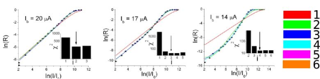
Figure 2: Measurement of the NbN nanodetector count rate as function of input power at Ib = 20 $\mu$A, Ib = 17 $\mu$A and Ib = 14 $\mu$A, fitted with the EPDC model (Eq. 1). The black squares represents the data points with error bars, the other lines represent fits, with the number of free parameters represented by the color of the line (see legend). Note that many of these lines overlap with each other and with the data. Insert: reduced $\chi^{2}$ of the fits as a function of number of parameters. For $I_{b}=14\mu A$ we have omitted the case $i=1$, where $\chi_{reduced}^{2}>10^{4}$. The arrows indicate the best fit. Note that in all three cases there are multiple fits which have similar reduced $\chi^{2}$, we reject the ones with superfluous free parameters for physical reasons.

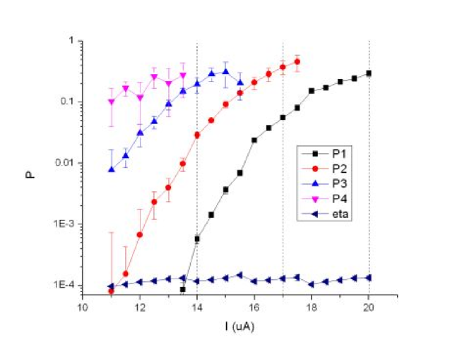
Figure 3: EPDC parameters and linear detection efficiency as function of bias current. This figure was obtained by repeatedly applying the method outlined in Section IV at various bias currents. The three dashed lines indicate the bias currents from Figure 3.

6 Discussion

The $p_{i}$ obtained from the fit represent the nonlinear action of our detection system, which is the physical property of interest. Since there are no other nonlinear elements in the detection system, we can unambiguously attribute the behaviour of the $p_{i}$ to the NbN nanodetector. It should be noted that result presented here is consistent with earlier results on these detectors [6], e.g. we reproduce the finding that the transitions between the various detection regimes (where the detector behaves approximately as an N-photon detector) are equally spaced in the current domain.

From Eq. 3, we can see that the response of the detector is given by terms of the form $p_{i}c_{i}(N)$, where $c_{i}(N)$ is the probability of having N photons. From this we can see that each $p_{i}$will be most dominant in the range of powers where the probability of having the corresponding number of photons is highest. For example, at 17 $\mu$A the detector has $p_{1}$= 0.06 and $p_{2}$= 0.37, meaning that at low powers ($\eta N<0.16$), where the one-photon contribution from the state is dominant, the detector will respond mostly to single photons, but at higher powers ($\eta N>0.16$) the response will be dominated by the two-photon events. This quantifies the change of detection regimes reported in measurements of count rate as a function of power [6].

The fitted linear detection efficiency $\eta$ fluctuates between $(9.6\pm 0.2)*10^{-5}$ and $(14.7\pm 0.6)*10^{-5}$. Normalizing to the estimated effective area of the detector of 100 nm by 150 nm and the beam size, we obtain an intrinsic detection efficiency of 8%. While it should be noted that this is only a rough estimate, it is higher than the value of 1% reported in [6], we attribute to the lower temperature of the experiment, at which NbN detectors are known to be more efficient [5].

It should be noted that since we combine all linear losses into a single parameter, we are unable to distinguish losses after the absorption event from those before the absoption event, provided they are linear. It is known for NbN meanders that not every absorbed photon causes a detection event [9]. However, since our measured linear loss does not depend on the bias current, it is reasonable to attribute it to optical loss and not to losses inside the detector. With the caveat that there may be a constant linear loss inside the detector, we can therefore conclude that the set of $p_{i}$ completely describes the behaviour of the detector.

7 Conclusion

We have introduced an extension of detector tomography which is applicable in the presence of a large linear loss. This detector characterization is of interest when using a quantum detector in a quantum optics or quantum communication experiment, since it gives a full prediction of the response of the detector to any incoming state. Furthermore, we have completely characterized the response of a superconducting nanodetector, over several operating regimes of the detector. This represents the first complete characterization of this type of detector, which is necessary for the use of this detector as a multiphoton subwavelength detector.

A second application of this characterization method is that it provides quantitative information about the response of the detector. Such quantitative characterization can also be used to test theoretical predictions of the response of the detector as a function of bias current [14], enabling further insight into the physics of the detection event in NbN photodetectors.

The idea of our formalism is to separate this linear loss from the nonlinear action of the detector. For the detector under study in this paper, this formalism completely describes the response of the detector. In contrast to earlier methods [15, 16] that assume a priori knowledge of the underlying detector physics, detector characterization based on the POVM formalism can be applied to any detector system without making assumptions about the operating principle of the detector [3, 4]. Therefore, the strength of the characterization applied here is that we can extract model-independent parameters that can be used to gain insight in the physics of photon detection with NbN detectors.

Finally, we comment on the applicability of our algorithm to other detectors: Effective Photon Detector Characterization shares the feature with detector tomography that it is as assumption-free as possible; making it possible to characterize a detector without any prior knowledge or model of the operational mechanism of the detector. The EPDC method has the added requirement that the detector saturates (i.e. always produces the same outcome) at some high input photon number. To our knowledge, this behaviour is generic to all quantum detectors constructed to date [17, 18, 16, 19]. It therefore does not represent an practical limitation.

8 Note

This work is part of the research programme of the Foundation for Fundamental Research on Matter (FOM), which is financially supported by the Netherlands Organisation for Scientific Research (NWO). JR would like to thank S. Jahanmiri Nejad for experimental advice.

References

- [1] E. Knill, R. Laflamme, and G. J. Milburn, “A scheme for efficient quantum computation with linear optics.” Nature 409, 46–52 (2001).
- [2] a. Feito, J. S. Lundeen, H. Coldenstrodt-Ronge, J. Eisert, M. B. Plenio, and I. a. Walmsley, “Measuring measurement: theory and practice,” New Journal of Physics 11, 093038 (2009).
- [3] J. S. Lundeen, a. Feito, H. Coldenstrodt-Ronge, K. L. Pregnell, C. Silberhorn, T. C. Ralph, J. Eisert, M. B. Plenio, and I. a. Walmsley, “Tomography of quantum detectors,” Nature Physics 5, 27–30 (2008).
- [4] M. K. Akhlaghi, A. H. Majedi, and J. S. Lundeen, “Nonlinearity in Single Photon Detection : Modeling and Quantum Tomography,” .
- [5] M. Hofherr, D. Rall, K. Ilin, M. Siegel, A. Semenov, H.-W. Hübers, and N. a. Gippius, “Intrinsic detection efficiency of superconducting nanowire single-photon detectors with different thicknesses,” Journal of Applied Physics 108, 014507 (2010).
- [6] D. Bitauld, F. Marsili, A. Gaggero, F. Mattioli, R. Leoni, S. J. Nejad, F. Lévy, and A. Fiore, “Nanoscale optical detector with single-photon and multiphoton sensitivity.” Nano letters 10, 2977–81 (2010).
- [7] G. N. Goltsman, O. Okunev, G. Chulkova, A. Lipatov, A. Semenov, K. Smirnov, B. Voronov, A. Dzardanov, C. Williams, and R. Sobolewski, “Picosecond superconducting single-photon optical detector,” Applied Physics Letters 79, 705 (2001).
- [8] I. Afek, O. Ambar, and Y. Silberberg, “High-NOON states by mixing quantum and classical light.” Science (New York, N.Y.) 328, 879–81 (2010).
- [9] A. J. Kerman, E. a. Dauler, J. K. W. Yang, K. M. Rosfjord, V. Anant, K. K. Berggren, G. N. Goltsman, and B. M. Voronov, “Constriction-limited detection efficiency of superconducting nanowire single-photon detectors,” Applied Physics Letters 90, 101110 (2007).
- [10] a. Gaggero, S. J. Nejad, F. Marsili, F. Mattioli, R. Leoni, D. Bitauld, D. Sahin, G. J. Hamhuis, R. Noetzel, R. Sanjines, and a. Fiore, “Nanowire superconducting single-photon detectors on GaAs for integrated quantum photonic applications,” Applied Physics Letters 97, 151108 (2010).
- [11] J. S. Lundeen, K. L. Pregnell, A. Feito, B. J. Smith, W. Mauerer, C. Silberhorn, J. Eisert, M. B. Plenio, and I. A. Walmsley, “A proposed testbed for detector tomography,” Physics pp. 1–9.
- [12] G. Brida, L. Ciavarella, I. P. Degiovanni, M. Genovese, L. Lolli, G. Mingolla, F. Piacentini, M. Rajteri, E. Taralli, and M. G. A. Paris, “Full quantum characterization of superconducting photon counters,” (2011).
- [13] T. Amri, “Quantum Behavior of Measurement Apparatus,” 8552, 1–20 (2010).
- [14] a. Semenov, a. Engel, H.-W. Hübers, K. Il’in, and M. Siegel, “Spectral cut-off in the efficiency of the resistive state formation caused by absorption of a single-photon in current-carrying superconducting nano-strips,” The European Physical Journal B 47, 495–501 (2005).
- [15] M. K. Akhlaghi and A. H. Majedi, “Semiempirical Modeling of Dark Count Rate and Quantum Efficiency of Superconducting Nanowire Single-Photon Detectors,” 19, 361–366 (2009).
- [16] A. Divochiy, F. Marsili, D. Bitauld, A. Gaggero, R. Leoni, F. Mattioli, A. Korneev, V. Seleznev, N. Kaurova, O. Minaeva, G. Gol’tsman, K. G. Lagoudakis, M. Benkhaoul, F. Lévy, and A. Fiore, “Superconducting nanowire photon-number-resolving detector at telecommunication wavelengths,” Nature Photonics 2, 302–306 (2008).
- [17] O. Haderka, M. Hamar, and J. Perina, “Experimental multi-photon-resolving detector using a single avalanche photodiode,” The European Physical Journal D Atomic Molecular and Optical Physics 28, 11 (2003).
- [18] P. P. Rohde, J. G. Webb, E. H. Huntington, and T. C. Ralph, “Photon number projection using non-number-resolving detectors,” New Journal of Physics 9, 233–233 (2007).
- [19] E. A. Dauler, A. J. Kerman, B. S. Robinson, J. K. W. Yang, B. Voronov, G. Gol’tsman, S. A. Hamilton, and K. K. Berggren, “Photon-number-resolution with sub-30-ps timing using multi-element superconducting nanowire single photon detectors,” Journal of Modern Optics 56, 13 (2008).