Causal modeling and inference for electricity markets

Abstract

How does dynamic price information flow among Northern European electricity spot prices and prices of major electricity generation fuel sources? We use time series models combined with new advances in causal inference to answer these questions. Applying our methods to weekly Nordic and German electricity prices, and oil, gas and coal prices, with German wind power and Nordic water reservoir levels as exogenous variables, we estimate a causal model for the price dynamics, both for contemporaneous and lagged relationships. In contemporaneous time, Nordic and German electricity prices are interlinked through gas prices. In the long run, electricity prices and British gas prices adjust themselves to establish the equlibrium price level, since oil, coal, continental gas and EUR/USD are found to be weakly exogenous.

1 Introduction

There is an ongoing debate on the convergence of and price dynamics in energy markets, and electricity markets in particular. For the US market, Park et al. (2006) use advances in causal flow modelling and find that the dynamic relationships between electricity markets not only are governed by transmission lines, but also by different market structure and regulation. Using similar techniques, the same authors indicate that the Canadian and US natural gas market is a single highly integrated market (Park et al., 2008). Mjelde and Bessler (2009) go one step further, and investigate how weekly dynamic price information flows among major US electricity generation fuel sources: natural gas, uranium, coal and crude oil. They find that peak electricity prices move natural gas prices, which in turn influence crude oil prices.

To our knowledge, price dynamics among Northern European electricity markets and their major fuel sources has not been closely looked into before. Zachmann (2008) rejects the hypothesis of full market integration of Northern European electricity markets. We will focus on the Nordic and German electricity markets (Weron, 2006). The Nordic electricity market (Nord Pool) is dominated by highly flexible hydro power (54% in 2007 (Fridolfsson and Tangerås, 2009)), and even though congestion within the Nord Pool area is not uncommon (Marckhoff and Wimschulte, 2009), we will consider the common Nordic system spot price here. The German EEX market, being the largest market in Europe, is on the other hand dominated by coal (47%) and nuclear power (23%) (Brunekreeft and Twelemann, 2005). Gas (17%), hydro and an increasing wind power production complement the picture. The EEX market is generally assumed to be less mature than the Nordic market (Weron, 2006; Weigt and von Hirschhausen, 2008; Müsgens, 2006; Fridolfsson and Tangerås, 2009).

We investigate the price dynamics between electricity prices and major fuel sources (oil, gas, coal) by estimating a causal model for the price dynamics, where Nordic water reservoir levels and German electricity production from wind mills are treated as exogenous variables. Mjelde and Bessler (2009) estimate a vector error correction model (VECM) for logarithmic prices. A directed acyclic graph (DAG) (Spirtes et al., 2000) representing instantaneous causal influences is then found from the resulting contemporaneous correlation matrix, using the greedy equivalence search (GES) algorithm of Chickering (2003).

Most causal DAG learning algorithms, including the GES algorithm, are based on the assumption that variables are jointly normally distributed. These methods share a fundamental problem: Several DAGs usually correspond to same joint distribution, so one only obtains an equivalence class of DAGs that are indistinguishable from data. While some directions of causal influences (edges in the DAG) may be the same for all DAGs in the equivalence class, usually many or most directions are left undetermined.

In the present paper, we rely on the assumption of non-normality, using the linear non-Gaussian acyclic model (LiNGAM) recently developed by Shimizu et al. (2006a, b). This allows us to identify one single DAG. Because of this, we are also able to coherently integrate both contemporaneous and time-lagged causal relationships into the same DAG analysis. For our data, the GES algorithm is only able to identify undirected contemporaneous associations. The LiNGAM approach, on the other hand, provides instantaneous and time-lagged directed causal influences.

2 Methods

The three basic building blocks of our data analysis are the vector autoregression (VAR) model, the vector error correction model (VECM) and the linear non-Gaussian acyclic model (LiNGAM) (Shimizu et al., 2006a, b). We will now describe each in turn, before we combine them to estimate both instantaneous and lagged causal effects.

2.1 Vector autoregression model

The vector autoregression model (Hamilton, 1994) is a standard tool of econometrics and multivariate time series analysis. Let the endogenous variables $\boldsymbol{x}_{t}$ and the exogenous variables $\boldsymbol{z}_{t}$ be observed random vectors depending on (time) $t=1,2,\ldots$. The basic idea of the VAR model is that the endogenous variables depend linearly on their $k$ previous values, as well as the current value of the exogenous variables, i.e.

$$\boldsymbol{x}_{t}=\boldsymbol{\mu}+\sum_{\tau=1}^{k}\boldsymbol{M}_{\tau}\boldsymbol{x}_{t-\tau}+\boldsymbol{\gamma}\boldsymbol{z}_{t}+\boldsymbol{e}_{t},$$ (1)

where $\boldsymbol{M}_{\tau}$ and $\boldsymbol{\gamma}$ are coefficient matrices of size $n\times n$ and $n\times d$, respectively, where $n$ is the number of endogenous variables and $d$ is the number of exogenous variables. Further, $\boldsymbol{\mu}$ is a constant vector and $\boldsymbol{e}_{t}$ is a vector of residuals (innovations).

All variables must have the same order of integration. If all variables are stationary, $I(0)$, we have the standard case of a VAR model. If all variables are non-stationary, $I(d)$, $d>1$, there are two possibilities. First, if the variables are not cointegrated, the variables must be differenced $d$ times in order to obtain a VAR. Second, if the variables are cointegrated, we may use a vector error correction model (VECM).

2.2 Vector error correction model

We here consider the case where the variables $\boldsymbol{x}_{t}$ are $I(1)$, so that they are differenced one time in order to achieve stationarity. The vector error correction model (VECM) can be derived from the VAR model in (1),

$$\Delta\boldsymbol{x}_{t}=\boldsymbol{\mu}+\boldsymbol{\Pi}\boldsymbol{x}_{t-1}+\sum_{\tau=1}^{k-1}\boldsymbol{\Gamma}_{\tau}\Delta\boldsymbol{x}_{t-\tau}+\boldsymbol{\gamma}\boldsymbol{z}_{t}+\boldsymbol{e}_{t},$$ (2)

where $\Delta$ is the difference operator ($\Delta\boldsymbol{x}_{t}=\boldsymbol{x}_{t}-\boldsymbol{x}_{t-1}$), and $\boldsymbol{\Gamma}_{\tau}$ is an $n\times n$ matrix relating changes in $\boldsymbol{x}_{t}$ for lagged $\tau$ periods to current changes in $\boldsymbol{x}_{t}$.

The matrix $\boldsymbol{\Pi}$ is called an error correction term, which compensates for the long-run information lost through differencing (Juselius, 2006). $\boldsymbol{\Pi}=\boldsymbol{\alpha}\boldsymbol{\beta}^{\prime}$, where $\boldsymbol{\alpha}$ and $\boldsymbol{\beta}$ are of dimensions $n\times r$, where the rank $r$ is the number of cointegration relationships. The $r$ linearly independent columns of $\boldsymbol{\beta}$ are the cointegrated vectors, each representing one long-run relationship between the series, and $\boldsymbol{\beta}^{\prime}\boldsymbol{x}_{t-1}$ is then stationary.

If $r=0$, the matrix $\boldsymbol{\Pi}$ does not exist, and we have a VAR in difference, not a VECM. If we have full rank, $r=n$, it does not make sense to specify the model as a VECM, as the stationary $\Delta\boldsymbol{x}_{t}$ in (2) will be equal to a non-stationary $\boldsymbol{\Pi}\boldsymbol{x}_{t-1}$ plus some lagged stationary variables and so on, which is inconsistent (Juselius, 2006).

Comparing (1) with (2) gives

$$\boldsymbol{\Pi}=\boldsymbol{\alpha}\boldsymbol{\beta}^{\prime}=-(\boldsymbol{I}-\sum_{\tau=1}^{k}\boldsymbol{M}_{\tau}),$$ (3)

and

$$\boldsymbol{\Gamma}_{\tau}=-\sum_{i=\tau+1}^{k}\boldsymbol{M}_{i}.$$ (4)

2.3 Linear non-Gaussian acyclic causal model

In general, a linear causal model on the zero-mean (centered) random variables $y_{i}$, $i=1,\ldots,m$, can be defined by

$$y_{i}=\sum_{k(i)<k(j)}\beta_{ij}y_{j}+\varepsilon_{i},$$ (5)

where the $\varepsilon_{i}$s are random noise terms and $k$ is a permutation over $\{1,\ldots,m\}$. We interpret $k$ as a causal ordering of the variables, where later variables cannot cause earlier variables. Equation (5) can be represented as a directed acyclic graph (DAG) with vertices corresponding to $y_{i}$ and edges corresponding to a nonzero $\beta_{ij}$. Estimating causal DAGs from observational data has received considerable interest in recent years (Pearl, 2000; Spirtes et al., 2000). For continuous $y_{i}$, standard methods assume that the noise terms $\varepsilon_{i}$ are jointly normally distributed, and use the estimated covariance matrix to infer the DAG.

Several methods for inferring DAGs from Gaussian observational data have been proposed. To enable comparison of our results and those of Park et al. (2008), we employ the Greedy Equivalence Search (GES) algorithm of Chickering (2003), as implemented in the software Tetrad IV (2004). The GES algorithm uses a score to evaluate how well a suggested DAG fits the data. Starting with an empty DAG, a greedy search over equivalence classes (defined below) is done. The search concludes when local maximum of the score is reached.

A general problem with the normality-based methods such as the GES algorithm is that, even with an infinite amount of data, one cannot identify a unique causal model (DAG), only a so-called Markov equivalence class consisting of several different DAGs corresponding to the same joint distribution. This is easily seen in the case of two variables $y_{1}$ and $y_{2}$, where there is clearly no way of distinguishing between the models $y_{1}\rightarrow y_{2}$ and $y_{1}\leftarrow y_{2}$ based on the covariance structure alone, and $\{y_{1}\rightarrow y_{2},y_{1}\leftarrow y_{2}\}$ is a Markov equivalence class. With three variables, the Markov equivalence classes are $\{y_{1}\rightarrow y_{2}\rightarrow y_{3},y_{1}\leftarrow y_{2}\leftarrow y_{3},y_{1}\leftarrow y_{2}\rightarrow y_{3}\}$ and $\{y_{1}\rightarrow y_{2}\leftarrow y_{3}\}$. For an extensive discussion of this problem, see Shimizu et al. (2006b).

In contrast, when assuming that the noise terms are independent and non-Gaussian, a unique causal structure is in fact identifiable. Equation (5) is then known as the LiNGAM (Shimizu et al., 2006a). Writing (5) in matrix form:

$$\boldsymbol{y}=\boldsymbol{B}\boldsymbol{y}+\boldsymbol{\varepsilon}$$ (6)

where $\boldsymbol{y}=(y_{1},\ldots,y_{m})^{\prime}$, $\boldsymbol{\varepsilon}=(\varepsilon_{1},\ldots,\varepsilon_{m})$ and $\boldsymbol{B}$ is the (permutable to lower triangular) matrix of coefficients $\beta_{ij}$. The independence of the elements of $\boldsymbol{\varepsilon}$ implies that there are ”no unobserved confounders” in the sense of Pearl (2000), so a causal interpretation is valid (cf. Shimizu et al. (2006a), Section 2). Letting $\boldsymbol{A}=(\boldsymbol{I}-\boldsymbol{B})^{-1}$, we can rewrite (6) as

$$\boldsymbol{y}=\boldsymbol{A}\boldsymbol{\varepsilon}.$$ (7)

Since the variables in $\boldsymbol{\varepsilon}$ are independent and non-Gaussian, (7) defines the Independent Component Analysis (ICA) model (Comon, 1994; Hyvärinen and Oja, 2000).

In ICA, the goal is to estimate both the so-called mixing matrix $\boldsymbol{A}$ and the independent components $\boldsymbol{\varepsilon}$. Essentially, in ICA we aim to find $\boldsymbol{A}$ and $\boldsymbol{\varepsilon}$ such that the entries of $\boldsymbol{\varepsilon}$ are as statistically independent as possible. By an argument based on the central limit theorem, this problem can also be posed as finding components which are as non-Gaussian as possible. Non-Gaussianity can be measured using the concept of entropy. The entropy of a random vector $\boldsymbol{y}$ with density $f$ is defined as $H(\boldsymbol{y})=-\int\!f(\boldsymbol{y})\log f(\boldsymbol{y})\mathrm{d}\boldsymbol{y}$. Among random variables with a given variance, Gaussian variables have the highest possible entropy. Therefore, we can measure non-Gaussianity based on negentropy $J$, which is defined by $J(\boldsymbol{y})=H(\boldsymbol{y}_{g})-H(\boldsymbol{y})$, where $\boldsymbol{y}_{g}$ is a Gaussian random vector having the same covariance matrix as $\boldsymbol{y}$. Clearly, $J(\boldsymbol{y})$ is zero for Gaussian $\boldsymbol{y}$ and positive for non-Gaussian $\boldsymbol{y}$. The iterative fixed-point algorithm fastICA (Hyvärinen, 1999) estimates $\boldsymbol{A}$ efficiently and robustly based on approximations to negentropy.

It can be seen from (7) that both $\boldsymbol{A}$ and $\boldsymbol{\varepsilon}$ can only be estimated up to a scaling constant and a permutation. However, both the scaling and the permutation can be found in the application of ICA to LiNGAM, as shown by Shimizu et al. (2006a). After estimating $\boldsymbol{A}$, the coefficient matrix $\boldsymbol{B}$ is immediately available as $\boldsymbol{I}-\boldsymbol{A}^{-1}$.

2.4 Combining instantaneous and lagged effects

Our interest is here in the following model:

$$\boldsymbol{x}_{t}=\boldsymbol{\mu}+\sum_{\tau=0}^{k}\boldsymbol{B}_{\tau}\boldsymbol{x}_{t-\tau}+\boldsymbol{\gamma}\boldsymbol{z}_{t}+\boldsymbol{\varepsilon}_{t}.$$ (8)

The difference between (8) and the VAR model defined in (1) is the inclusion of instantaneous causal effects $\boldsymbol{B}_{0}$, where the matrix $\boldsymbol{B}_{0}$ corresponds to a DAG (i.e., can be permuted to strict lower triangularity) as in Section 2.3. $\boldsymbol{B}_{1},\boldsymbol{B}_{2},\ldots$ contain autoregressive effects, and their corresponding graphs may be cyclic.

To estimate the model in (8), we customise the method described by Hyvärinen et al. (2008):

1. Estimate a VECM model for the data, see (2). We here obtain the coefficient matrices $\widehat{\boldsymbol{\Pi}}$ and $\widehat{\boldsymbol{\Gamma}}_{1},\ldots,\widehat{\boldsymbol{\Gamma}}_{k-1}$, together with $\widehat{\boldsymbol{\mu}}$ and $\widehat{\boldsymbol{\gamma}}$.

2. Translate the estimated VECM coefficients into a VAR representation, see (3) and (4). We then obtain the coefficient matrices $\widehat{\boldsymbol{M}}_{1},\ldots,\widehat{\boldsymbol{M}}_{k}$ in (1).

3. Compute the residuals $\widehat{\boldsymbol{e}}_{t}$,

   $$\widehat{\boldsymbol{e}}_{t}=\boldsymbol{x}_{t}-\widehat{\boldsymbol{\mu}}-\widehat{\boldsymbol{\gamma}}\boldsymbol{z}_{t}-\sum_{\tau=1}^{k}\widehat{\boldsymbol{M}}_{\tau}\boldsymbol{x}_{t-\tau}.$$ (9)

4. Perform the LiNGAM analysis on the residuals to find an estimate of the instantaneous effect matrix $\boldsymbol{B}_{0}$. This matrix is a solution to the model

   $$\widehat{\boldsymbol{e}}_{t}=\boldsymbol{B}_{0}\widehat{\boldsymbol{e}}_{t}+\tilde{\boldsymbol{\varepsilon}}_{t}.$$ (10)

   See Section 2.3 for details.

5. Compute the matrices of lagged causal effects, $\boldsymbol{B}_{\tau}$, $\tau>0$, which are given as

   $$\widehat{\boldsymbol{B}}_{\tau}=(\boldsymbol{I}-\boldsymbol{B}_{0})\widehat{\boldsymbol{M}}_{\tau}.$$ (11)

How do we find (11)? Equation (8) gives

$$(\boldsymbol{I}-\boldsymbol{B}_{0})\boldsymbol{x}_{t}=\boldsymbol{\mu}+\sum_{\tau=1}^{k}\boldsymbol{B}_{\tau}\boldsymbol{x}_{t-\tau}+\boldsymbol{\gamma}\boldsymbol{z}_{t}+\boldsymbol{\varepsilon}_{t}.$$

This gives

$$\begin{split}\boldsymbol{x}_{t}=&\ (\boldsymbol{I}-\boldsymbol{B}_{0})^{-1}\boldsymbol{\mu}+\sum_{\tau=1}^{k}(\boldsymbol{I}-\boldsymbol{B}_{0})^{-1}\boldsymbol{B}_{\tau}\boldsymbol{x}_{t-\tau}\\ &+(\boldsymbol{I}-\boldsymbol{B}_{0})^{-1}\boldsymbol{\gamma}\boldsymbol{z}_{t}+(\boldsymbol{I}-\boldsymbol{B}_{0})^{-1}\boldsymbol{\varepsilon}_{t}.\end{split}$$ (12)

Comparing (12) with (1), we find that $(\boldsymbol{I}-\boldsymbol{B}_{0})^{-1}\boldsymbol{B}_{\tau}=\boldsymbol{M}_{\tau}$ for $\tau\geq 1$. Also, we see that $(\boldsymbol{I}-\boldsymbol{B}_{0})^{-1}\boldsymbol{\varepsilon}_{t}=\boldsymbol{e}_{t}$, which gives rise to (10).

2.5 Time-lagged causal flow and Granger causality

One may ask whether a time-lagged causal flow is different from Granger causality. Granger causality is the ability to reduce the prediction error (Hamilton, 1994). Based on the VAR representation (1), a variable $i$ Granger causes the variable $j$ if at least one of the coefficients of $\boldsymbol{M}_{\tau}$ from $\boldsymbol{x}_{t-\tau}^{(i)}$, $\tau\geq 1$, to $\boldsymbol{x}_{t-\tau}^{(j)}$ is significantly non-zero, since this reduces the prediction error in $\boldsymbol{x}_{t}^{(j)}$. Hyvärinen et al. (2008) proposed a combined definition of Granger causality: If at least one of the coefficients $\boldsymbol{B}_{\tau}(j,i)$, $\tau\geq 0$, is significantly non-zero, variable $i$ causes $j$. See Hyvärinen et al. (2008) and Zhang and Hyvärinen (2009) for a more thorough discussion.

3 Data

We focus on the Nordic and German electricity markets, their major fuel sources (gas, coal, oil) and physical variables known to partly explain Nordic and German electricity prices; German wind power production and Nordic water reservoir levels. The data consist of 365 weekly observations of each variable from 2002–2008. Ideally, we should have used data further back. However, firstly, the wind data were not available until 2002. Secondly, six years is a long time in quite rapidly evolving and increasingly integrated European gas and electricity markets (Zachmann, 2008; Bunn and Gianfreda, 2010; Ruperez Micola and Bunn, 2007). The markets were less mature further back, but if wind data had been available, we could have included 2001 data as well.

All price series are given in or converted to EUR. Transforming all prices to a common currency (Hovanov et al., 2004) could induce dependencies related to exchange rate fluctuations and not energy price fluctuations. For that reason, and since exchange rates may also influence commodity prices (Chen and Chen, 2007; Akram, 2009; Zhang et al., 2008), we include the EUR/USD exchange rate as well.

All price series are given as averages over the week, since the producers try to maximise the accumulated income and buyers are likewise minimising their accumulated expenses. Had we instead considered, say, the hourly price at hour 24 each Sunday, our results would not necessarily say much about price information flow between the weekly price levels.

An overview of the data is given in Table 1, and they are displayed in Figure 1–3.

We have included two gas prices here: Zeebrügge and NBP, representing continental Europe and the United Kingdom, respectively. A few other gas markets are more relevant for the German electricity market than the Zeebrügge gas market, but the historic data period is then not long enough. The Zeebrügge and NBP gas markets are connected through the Bacton–Zeebrügge interconnector (Ruperez Micola and Bunn, 2007). We expect the Zeebrügge gas market to be more important than the NBP market for the electricity price formation, since it is closer to the German (and Nordic) market.

We will treat German wind and Nordic reservoir levels as exogenous variables in (2), which to some extent is debatable. The electricity market does not influence the wind itself, but may have contributed to the long term increase in wind power mills. Similarly, the electricity market does not influence the inflow into water reservoirs, but the water reservoirs are ideally used when prices are high. Still, we find it most correct to treat these two variables as exogenous.

All time series, except reservoir levels, were log-transformed. Since the reservoir levels are bounded by 0 and 100%, they were logit-transformed. Next, all transformed variables except the oil price, were seasonally adjusted by subtracting a seasonal term

$$\lambda_{t}=\beta^{(0)}+\sum_{j=1}^{2}{\beta^{(1)}_{j}\sin\left(\frac{2\pi jt}{52}\right)+\beta^{(2)}_{j}\cos\left(\frac{2\pi jt}{52}\right),}$$

which was estimated by least squares regression. This was done in order to have variables that represent deviations from a normal level.

Data	Description	Resolution
Nordic el. price	Nord Pool system	Weekly, average spot price
German el. price	European Energy Exchange (EEX)	Weekly, average spot price
Oil price	Brent crude, International	Weekly, average spot price
	Petroleum Exchange (IPE)
Gas price 1	National balancing point	Weekly, average spot price
	(NBP), UK
Gas price 2	Zeebrügge, Belgium	Weekly, average spot price
Coal price	CIF ARA, Northwest Europe	Weekly, average physical price
EUR/USD	Exchange rate	Weekly, average rate
Water Nordic	Reservoir levels, Norway+Sweden	Values for each Monday
Wind Germany	Electricity production, wind plants	Weekly, average production

Table 1: Data overview. The data range from the first week of 2002 to the last week of 2008, in total 365 weekly values for each of the variables. Since German wind production is not publicly available, the German wind production data were calculated by Point Carbon (http://www.pointcarbon.com).

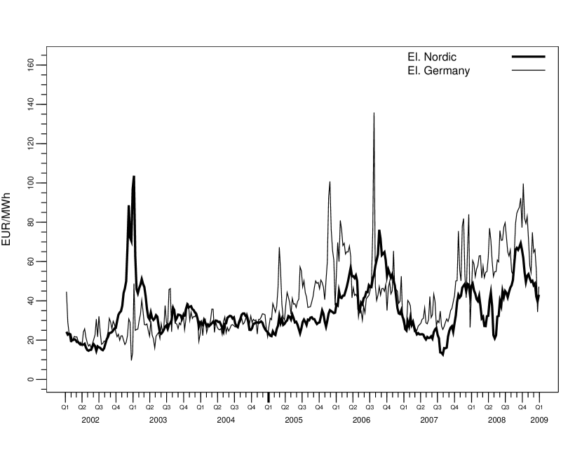
Figure 1: Weekly electricity spot prices, Nordic and German.

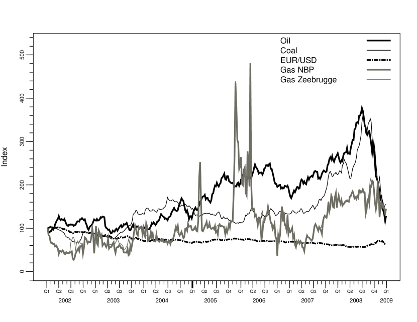
Figure 2: Weekly oil, coal and gas prices, and the EUR/USD exchange rate. All price series are given in Euro and indexed to 100 at Week 1 January 2002.

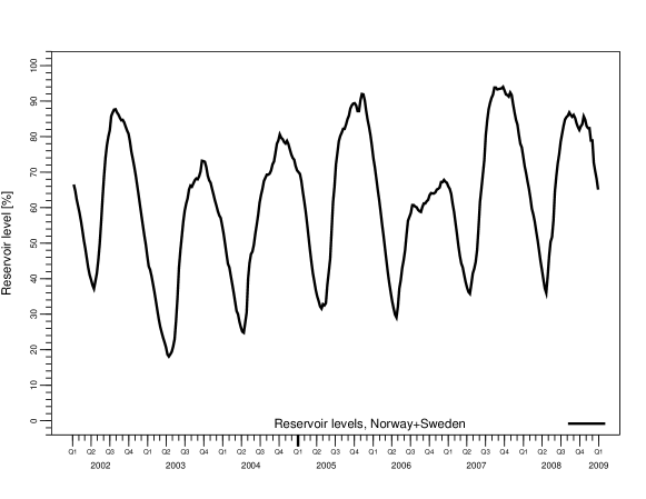
(a) Water reservoir levels, Nordic (Norway+Sweden).

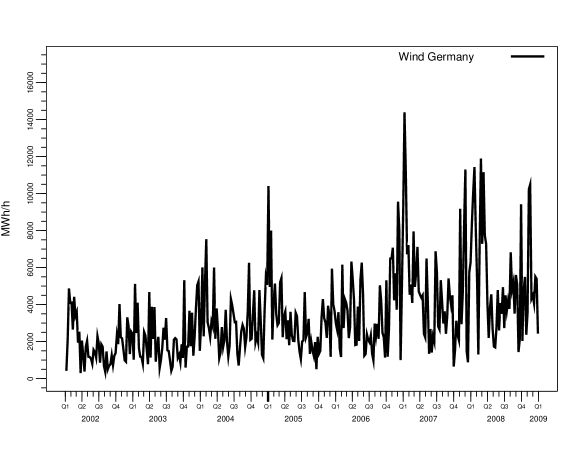
(b) Electricity production from wind plants in Germany.

Figure 3: Weekly values of exogenous variables.

4 Results

4.1 Time series analysis

Using the criteria of Akaike, Schwarz and Hannan and Quinn (Claeskens and Hjort, 2008), the optimal lag order of the unrestricted VAR with the two exogenous variables (1) was found to be two (Table 2), even though Akaike’s criterion was almost as good for three lags. Phillip-Perron unit root tests indicate that there is no evidence for stationarity of the series Oil, EURUSD and Coal. The same tests performed on the first differences indicate that these are stationary. Table 3 shows the test statistics and the p-values for each of the series.

	Lag order
Model selection criterion	1	2	3	4	5
Akaike	-38.96	-39.55	-39.54	-39.51	-39.38
Hannan and Quinn	-38.65	-39.03	-38.81	-38.57	-38.23
Schwarz	-38.19	-38.25	-37.71	-37.14	-36.48

Table 2: Akaike, Schwarz and Hannan and Quinn model selection criteria for the optimal lag order of the VAR with a constant.

	Original data		First differences
	statistic	p-value	statistic	p-value
ElNordic	-3.6685	0.0050	-14.5090	0.0000
ElGermany	-4.5652	0.0002	-26.8163	0.0000
Oil	-1.5193	0.5229	-15.2474	0.0000
EURUSD	-2.1031	0.2437	-14.9070	0.0000
Coal	-1.3370	0.6132	-10.8962	0.0000
GasNBP	-3.1755	0.0223	-23.8243	0.0000
GasZEE	-3.0617	0.0304	-23.2813	0.0000

Table 3: Stationarity test using the Phillip-Perron unit root test: Test statistics for both the original time series (on log scale) and the first differences of the time series (on log scale), when testing for stationarity. The null hypothesis is that the series has a unit root, i.e. that they are non-stationary.

We have also used another test of stationarity, the KPSS test (Kwiatkowski et al., 1992), where the null hypothesis is that each of the series is stationary. All time series, except for ElNordic, are rejected at a $1\%$ significance level. ElNordic is rejected at a $5\%$ significance level. The KPSS test on first differences indicate that all time series are level-stationary when differenced.

We use the trace test to determine the number of cointegrating vectors, and the Schwarz criterion for determining whether the constant is within or outside the cointegration space. The trace test indicates that there are three cointegrated vectors at a $1\%$ significance level, and the Schwarz criterion indicates that the constant is inside the cointegrating space. Table LABEL:tab:coint-const shows the test statistics and the critical values for different ranks when the constant is within the cointegration space. Table 5 shows the Schwarz criterion for the constant within and outside the cointegration space, when the cointegration rank is three. Since the cointegration tests can be sensitive to the lag structure of the VAR (Kasa, 1992), we have repeated the trace test for up to five lags in the VAR. In any case, and regardless of whether the constant is within or outside the cointegration space, we conclude that the number of cointegrating vectors is three.

Table 4: Trace test of cointegration, when the constant is within the cointegration space.

Rank	Trace test	Critical values
(r)	statistic	$10\%$	5%	1%
$r\leq 6$	3.72	7.52	9.24	12.97
$r\leq 5$	13.92	17.85	19.96	24.60
$r\leq 4$	29.39	32.00	34.91	41.07
$r\leq 3$	59.77	49.65	53.12	60.16
$r\leq 2$	102.23	71.86	76.07	84.45
$r\leq 1$	172.97	97.18	102.14	111.01
$r=0$	280.18	126.58	131.70	143.09

	Schwarz loss
Constant within	-3487.45
Constant outside	-3482.29

Table 5: The Schwarz loss when the constant is inside and outside the cointegration space, for the case of three cointegrated vectors.

A cointegrating vector is a stationary linear combination of possibly non-stationary vector time-series components. This combination might consist of only one of the series, which then must be stationary. It is interesting to test if this is the case, especially since the Phillip-Perron test suggests that several of the series are stationary. Table 6 shows the p-values of this test applied to each of the series, whose null hypothesis is that the series is by itself one of the cointegrating vectors. We see that all series are rejected, indicating that none of the cointegrating vectors consist of only one of the series.

	P-value
ElNordic	0.0005
ElGermany	0.0000
Oil	0.0000
EURUSD	0.0000
Coal	0.0000
GasNBP	0.0002
GasZEE	0.0001

Table 6: Test of whether a series by itself is one of the cointegrating vectors.

After fitting a VEC model with rank three to our data, see (2), we perform a normality test on the residuals. We use the Jarque-Bera test which tests for normality in both the univariate and multivariate case. The test rejects the null hypothesis of normality for each univariate series and for the multivariate case as well. In addition, an investigation of the residuals showed no significant auto-correlation between the residuals. Thus, the assumption of independent and non-Gaussian residuals is not unreasonable, and LiNGAM can be used.

A weak exogeneity test is performed, which tests the null hypothesis that each of the series does not respond to disturbances or shocks in the cointegration space, i.e. that the series is unresponsive to the deviations from the long-run relationships. This test is performed on $\boldsymbol{\alpha}$, more specifically, for one particular series, we test whether the corresponding row in $\boldsymbol{\alpha}$ (and hence in $\boldsymbol{\Pi}$) is zero.

Further, an exclusion test is performed, which tests the null hypothesis that a particular series is not in the cointegration space. This test is performed on $\boldsymbol{\beta}$, also here testing for a zero row. For more details on tests on $\boldsymbol{\alpha}$ and $\boldsymbol{\beta}$, see e.g. Juselius (2006).

Table 7 shows the p-values for both the weak exogeneity test and the exclusion test. We see that ElNordic, ElGermany and GasNBP are rejected at a $3\%$ or lower significance level in the weak exogeneity test, meaning that the long-run relationships in the data are important for these series, whereas for the other series there is not evidence for this. In the exclusion test, ElNordic, ElGermany, EURUSD, GasNBP and GasZEE are rejected. Hence, there is strong evidence that these series are included in the long-run relationships. An exclusion test is also performed on the constant term, which results in a rejection of the null hypothesis at a $2\%$ significance level. This agrees with the Schwarz conclusion in Table 5.

	Weak exogeneity	Exclusion
ElNordic	0.0065	0.0001
ElGermany	0.0000	0.0000
Oil	0.3722	0.1458
EURUSD	0.8023	0.0019
Coal	0.5012	0.1388
GasNBP	0.0298	0.0000
GasZEE	0.1866	0.0000

Table 7: The p-values for the weak exogeneity test and the exclusion test, whose null hypothesis is that a particular series does not respond to shocks in the cointegration space, and that a particular series is not in the cointegration space, respectively.

Figure 4 displays the impulse responses for all series, i.e. the responses of each series to a shock in each series. Each column shows the up to ten week responses of all series caused by an impulse (a one-time-only shock) in one of the series (the column headers show the impulses, whereas the row headers show the responses). The responses are normalised so that they can be compared with each other.

In order to get the impulse responses, the causal ordering among variables is needed. For Figure 4, we have followed the standard approach and used Bernanke ordering (Bernanke, 1986). The innovations are written as a function of more fundamental, internally orthogonal sources of variation, $\boldsymbol{\nu}_{t}$, given by $\boldsymbol{e}_{t}=\widetilde{\boldsymbol{A}}^{-1}\boldsymbol{\nu}_{t}$, where $\widetilde{\boldsymbol{A}}$ is a matrix representing how the innovations $\boldsymbol{e}_{t}$ are caused by orthogonal variation in each variable. Alternatively, we could here have used our LiNGAM based ordering.

As seen on the diagonal, all series respond positively to their own shocks, and except for EURUSD, these responses are also strong. ElGermany responds quickly and strongly to shocks in ElNordic, whereas there is not much impulse response the other way around. GasNBP and GasZEE have a slowly increasing response to a shock in ElNordic, whereas they respond much quicker to a shock in ElGermany.

ElNordic is mostly affected by impulses in GasNBP and GasZEE, and also here, these responses are slowly increasing over time. Besides being affected by impulses in ElNordic, ElGermany is also affected by impulses in GasNBP and GasZEE. The response caused by a shock in GasNBP is much quicker for ElGermany than for ElNordic. Further, GasZEE is more affected by a shock in GasNBP than the other way around.

Finally, we see that Oil, EURUSD and Coal are neither causing any significant responses in the other series, nor responding to shocks in any of the other series.

Figure 4: Impulse response plot: Each column shows the up to ten week responses in all series to a one-time-only shock in the series listed in the column header.

4.2 Learning contemporaneous and time-lagged causal DAGs

In the following we investigate the instantaneous causal ($\boldsymbol{B}_{0}$) and lagged ($\boldsymbol{B}_{1}$ and $\boldsymbol{B}_{2}$) effects.

The time series were standardised before the following DAG analysis, enabling direct comparison of the strengths of causal effects. $\boldsymbol{B}_{0}$, $\boldsymbol{B}_{1}$ and $\boldsymbol{B}_{2}$ were then estimated as described in Section 2.4. Insignificant edges of $\boldsymbol{B}_{0}$ were removed using the resampling method described in Section 6.3 of Shimizu et al. (2006a). As seen in (11) in Section 2.4, the time-lagged effects $\boldsymbol{B}_{\tau},\tau=1,2$, depend on both $\boldsymbol{B}_{0}$ and the matrix $\boldsymbol{M}_{\tau}$ of pure autoregressive effects. Therefore, the resampling method used for $\boldsymbol{B}_{0}$ is not available for the time-lagged effects, and it is not clear from Equation (11) how we could assess significance e.g. using p-values. However, since the data are standardised, we may simply use a cutoff in effect size as our significance threshold. We have chosen to remove all effects from $\boldsymbol{B}_{1}$ and $\boldsymbol{B}_{2}$ that are smaller in absolute value than the $70\%$ absolute value quantile of all the elements in $\boldsymbol{B}_{1}$.

To illustrate the advantages of the use of the LiNGAM methodology, we show instantaneous effects estimated using the GES algorithm, as implemented in Tetrad IV (2004). The results are shown in the partially directed acyclic graph (PDAG) in Figure 5. The PDAG shows the entire equivalence class as a single graph. Having a directed edge in the PDAG means that this edge has the same orientation for all DAGs in the equivalence class. Undirected edges in the PDAG have different orientations for different members of the Markov equivalence class. Note that the PDAG in Figure 5 is completely undirected, so no directions of causal influences can be determined in this case. Figure 5 shows an association between the coal price and the EURUSD. No price information seems to flow to or from the oil price, while the Nordic and German electricity prices seem to be connected through the two gas prices.

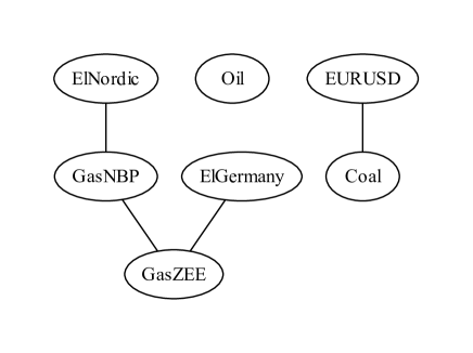
Figure 5: The instantaneous causal effects obtained using the GES algorithm in Tetrad IV (2004).

Figure 6 shows the graphical representation of $\boldsymbol{B}_{0}$, estimated using LiNGAM, as described in Section 2.4. Most of these instantaneous effects are intuitively reasonable. The main difference between the DAG $\boldsymbol{B}_{0}$ and the PDAG obtained using the GES algorithm in Figure 5 is that the latter lacks directions of the edges. Again, information does not flow to/from the oil price. As expected, the arrow goes from EURUSD to coal prices. Information flows from GasZEE to GasNBP, ElNordic and ElGermany. This is partly surprising, but we should keep in mind that the Nordic reservoir levels and German wind have already been accounted for in the model, and it might be that, contemporaneously, GasZEE plays an important role.

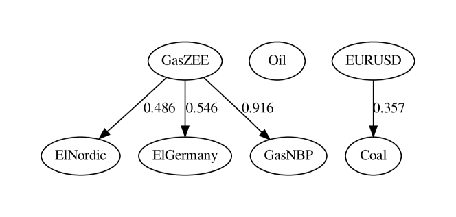
Figure 6: $\boldsymbol{B}_{0}$: The instantaneous causal effects.

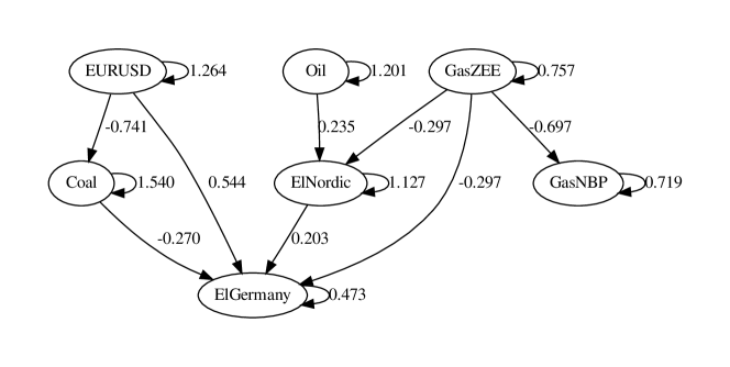
Figure 7: $\boldsymbol{B}_{1}$: The causal effects with lag one. The smallest effects have been removed.

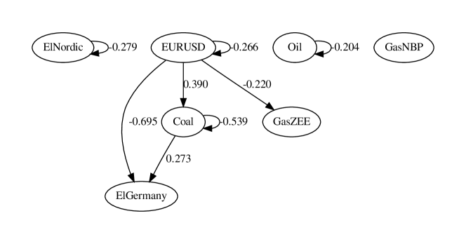
Figure 8: $\boldsymbol{B}_{2}$: The causal effects with lag two. The smallest effects have been removed.

Figure 7 and 8 show the graphical representations of $\boldsymbol{B}_{1}$ and $\boldsymbol{B}_{2}$, respectively. Note that these graphs are directed, but cyclic, so they are not DAGs. This is natural for time-lagged relationships. We see that all variables influence themselves at time lag one, and that ElNordic, EURUSD, Coal and Oil even influence themselves at time lag two.

At lag one ($\boldsymbol{B}_{1}$), ElGermany is (mainly) influenced directly and indirectly by EURUSD and GasZEE, indirectly by Oil, and directly by Coal and ElNordic. GasNBP is influenced by GasZEE (and GasNBP itself), but influences nothing else. Note, however, that some of the effects are quite small, except for the EURUSD $\rightarrow$ Coal, EURUSD $\rightarrow$ ElGermany and GasZEE $\rightarrow$ GasNBP relationships. At lag two ($\boldsymbol{B}_{2}$), there are fewer strong effects, except that EURUSD seems to play an important role.

5 Discussion

Using time series models combined with new advances in causal inference, we have studied how dynamic price information flows among Northern European electricity spot prices and prices of major electricity generation fuel sources. Applying our methods to weekly Nordic and German electricity prices, and oil, gas and coal prices, as well as German wind power and Nordic water reservoir levels, we have estimated a causal model for the price dynamics, both for contemporaneous and lagged relationships.

We find that the oil price, coal price and EUR/USD exchange rate are non-stationary, while Nordic and German electricity prices, as well as British and Zeebrügge gas prices are stationary. Our results can be compared with the results from Mjelde and Bessler (2009), who study the US market, even though we have treated Nordic water reservoir levels and German wind power as exogenous variables. There are a few noteworthy similarities and differences. Mjelde and Bessler include both peak, and off-peak prices, while we consider base prices. Note, however, that the peak/off-peak difference in the Nordic electricity market is less pronounced due to the very flexible hydro power. Contrary to Mjelde and Bessler, we find only positive innovation shock responses, for example from natural gas to coal, where there is a negative response in the US study. We both find a strong connection between gas and electricity prices. In contemporaneous time, we find a causal link from (Zeebrügge) gas prices to the electricity markets, while the US study gives the opposite conclusion. We find that coal and EURUSD together stand alone in contemporaneous time. In the US study, where the exchange rate is not included in the analysis (since all prices are in USD), coal stands alone in contemporaneous time. We find that even oil stands alone in contemporaneous time, which could be explained by the difference in European and US gas markets (Hobæk Haff et al., 2008), even though they may converge due to the increase in liquefied natural gas trade (Neumann, 2009). As with Mjelde and Bessler (2009), we find that all price series are cointegrated with a few cointegrating vectors (three in our case). At longer horizons, electricity prices and British gas prices adjust themselves to establish the equilibrium price level, since oil, coal, continental gas and EUR/USD are found to be weakly exogenous. In our analysis, however, and contrary to the US study, the exclusion test casts some doubt on whether the oil and coal prices are part of the cointegrating space.

Generally, the British gas prices are not important for the electricity markets when the Zeebrügge gas price is included, which is expected, since the Zeebrügge gas market is closer to the electricity generation and grid. The fact that coal prices do not play an important role in contemporaneous time in our analysis, while gas does, could first of all be because we have employed the more liquid CIF ARA price, while local producers may pay a different price, which may also partly be the case for the Zeebrügge gas prices. Second, the coal price has a low volatility compared to the gas and electricity prices, and naturally reacts more slowly to peak demand, since the coal prices’ influence is affected by transportation time and costs. Third, there has been speculation that the oil and gas markets in Europe are decoupling (see e.g. Panagiotidis and Rutledge (2007)), which could also partly explain why the oil and gas prices play different roles in this Northern European commodity price game.

In our view, there are two main methodological advantages of our approach, as compared to previous work (Mjelde and Bessler, 2009; Park et al., 2006, 2008). First, we are able to identify one unique contemporaneous graph, as opposed to a Markov equivalence class (which might be large). Second, we are able to properly and coherently deal with both instantaneous and time-lagged effects in the same analysis. Park et al. (2006) (p. 97) state that “in contrast to the directed graph analysis, forecast error variance decomposition and impulse response functions allow for analysis of dynamic information flows over time”, i.e. in their view, DAGs are only applicable for analysing instantaneous effects. We have shown that DAGs are in fact useful for combining time-lagged and instantaneous effects.

Implicit in our premise of statistically independent errors/residuals is the assumption of having no unobserved confounders: Any unmeasured common cause of any two of our variables would skew our results and create a dependence. It is possible to include latent variables in the LiNGAM model (Hoyer et al., 2008), but we have seen this as out of the scope of our paper, due to the added complications of dealing with time series data.

Our approach is a first attempt at a causal model for the price dynamics, and can be improved in many ways. Future work could include non-linear causal discovery (Hoyer et al., 2009), incorporating possible effects of stochastic volatility and investigating the price dynamics on a finer time scale, for example with daily instead of weekly price series.

Acknowledgements

This work is funded by Statistics for Innovation, (sfi)², one of the 14 Norwegian Centres for Research-based Innovation. We thank Norsk Hydro for supplying the data, and in particular Rønnaug Sægrov Mysterud for useful discussions. We are grateful to Arnoldo Frigessi for helpful comments. We appreciate Patrik O. Hoyer’s help with the LiNGAM methodology and software.

References

- Akram (2009) Akram, Q. F., 2009. Commodity prices, interest rates and the dollar. Energy Economics 31 (6, Sp. Iss. SI), 838–851.
- Bernanke (1986) Bernanke, B. S., 1986. Alternative explanations of the money-income correlation. In: Carnegie-Rochester Conference on Public Policy 25. pp. 49–99.
- Brunekreeft and Twelemann (2005) Brunekreeft, G., Twelemann, S., 2005. Regulation, competition and investment in the German electricity market: RegTP or REGTP. Energy Journal, 99–126.
- Bunn and Gianfreda (2010) Bunn, D. W., Gianfreda, A., MAR 2010. Integration and shock transmissions across European electricity forward markets. Energy Economics 32 (2), 278–291.
- Chen and Chen (2007) Chen, S.-S., Chen, H.-C., 2007. Oil prices and real exchange rates. Energy Economics 29 (3), 390–404.
- Chickering (2003) Chickering, D. M., 2003. Optimal structure identification with greedy search. Journal of Machine Learning Research 3 (3), 507–554.
- Claeskens and Hjort (2008) Claeskens, G., Hjort, N. L., 2008. Model Selection and Model Averaging. Cambridge University Press.
- Comon (1994) Comon, P., 1994. Independent component analysis – a new concept? Signal Processing 36, 287–314.
- Fridolfsson and Tangerås (2009) Fridolfsson, S. O., Tangerås, T. P., 2009. Market power in the Nordic electricity wholesale market: A survey of the empirical evidence. Energy Policy 37 (9), 3681–3692.
- Hamilton (1994) Hamilton, J. D., 1994. Time Series Analysis. Princeton University Press.
- Hobæk Haff et al. (2008) Hobæk Haff, I., Lindqvist, O., Løland, A., 2008. Risk Premium in the UK Natural Gas Forward Market. Energy Economics, 2420–2440.
- Hovanov et al. (2004) Hovanov, N., Kolari, J., Sokolov, M., JUN 2004. Computing currency invariant indices with an application to minimum variance currency baskets. Journal of Economic Dynamics & Control 28 (8), 1481–1504.
- Hoyer et al. (2009) Hoyer, P. O., Janzing, D., Mooij, J., Peters, J., Schölkopf, B., 2009. Nonlinear causal discovery with additive noise models. In: Advances in Neural Information Processing Systems 21. Proceedings of the 2008 Conference. pp. 689–696.
- Hoyer et al. (2008) Hoyer, P. O., Shimizu, S., Kerminen, A. J., Palviainen, M., 2008. Estimation of causal effects using linear non-Gaussian causal models with hidden variables. International Journal of Approximate Reasoning 49, 362–378.
- Hyvärinen (1999) Hyvärinen, A., 1999. Fast and robust fixed-point algorithms for independent component analysis. IEEE Transactions on Neural Networks 10 (3), 626–634.
- Hyvärinen and Oja (2000) Hyvärinen, A., Oja, E., 2000. Independent component analysis: algorithms and applications. Neural networks 13 (4-5), 411–430.
- Hyvärinen et al. (2008) Hyvärinen, A., Shimizu, S., Hoyer, P., 2008. Causal modelling combining instantaneous and lagged effects: an identifiable model based on non-Gaussianity. In: Proceedings of the 25th international conference on Machine learning. ACM New York, NY, USA, pp. 424–431.
- Juselius (2006) Juselius, K., 2006. The Cointegrated VAR model. Oxford University Press.
- Kasa (1992) Kasa, K., FEB 1992. Common stochastic trends in international stock markets. Journal of Monetary Economics 29 (1), 95–124.
- Kwiatkowski et al. (1992) Kwiatkowski, D., Phillips, P. C. B., Schmidt, P., Shin, Y., 1992. Testing the Null Hypothesis of Stationarity against the Alternative of a Unit Root. Journal of Econometrics 54, 159–178.
- Marckhoff and Wimschulte (2009) Marckhoff, J., Wimschulte, J., 2009. Locational price spreads and the pricing of contracts for difference: Evidence from the Nordic market. Energy Economics 31 (2), 257–268.
- Mjelde and Bessler (2009) Mjelde, J. W., Bessler, D. A., 2009. Market integration among electricity markets and their major fuel source markets. Energy Economics 31 (3), 482–491.
- Müsgens (2006) Müsgens, F., 2006. Quantifying market power in the German wholesale electricity market using a dynamic multi-regional dispatch model. Journal of Industrial Economics 54 (4), 471–498.
- Neumann (2009) Neumann, A., 2009. Linking Natural Gas Markets – Is LNG Doing its Job? Energy Journal Sp. Iss. SI, 187–199.
- Panagiotidis and Rutledge (2007) Panagiotidis, T., Rutledge, E., 2007. Oil and gas markets in the UK: Evidence from a cointegrating approach. Energy Economics 29 (2), 329–347.
- Park et al. (2006) Park, H., Mjelde, J., Bessler, D., 2006. Price dynamics among US electricity spot markets. Energy Economics 28 (1), 81–101.
- Park et al. (2008) Park, H., Mjelde, J., Bessler, D., 2008. Price interactions and discovery among natural gas spot markets in North America. Energy Policy 36 (1), 290–302.
- Pearl (2000) Pearl, J., 2000. Causality: Models, Reasoning and Inference. Cambridge University Press.
- Ruperez Micola and Bunn (2007) Ruperez Micola, A., Bunn, D. W., 2007. Two markets and a weak link. Energy Economics 29 (1), 79–93.
- Shimizu et al. (2006a) Shimizu, S., Hoyer, P., Hyvärinen, A., Kerminen, A., 2006a. A linear non-Gaussian acyclic model for causal discovery. The Journal of Machine Learning Research 7, 2003–2030.
- Shimizu et al. (2006b) Shimizu, S., Hyvärinen, A., Hoyer, P., Kano, Y., 2006b. Finding a causal ordering via independent component analysis. Computational Statistics and Data Analysis 50 (11), 3278–3293.
- Spirtes et al. (2000) Spirtes, P., Glymour, C., Scheines, R., 2000. Causation, Prediction, and Search. The MIT Press, Cambridge, MA.
-
Tetrad IV (2004)
Tetrad IV, 2004. Tetrad IV manual.
URL http://www.phil.cmu.edu/projects/tetrad/tetrad4.html - Weigt and von Hirschhausen (2008) Weigt, H., von Hirschhausen, C., 2008. Price formation and market power in the German wholesale electricity market in 2006. Energy Policy 36 (11), 4227–4234.
- Weron (2006) Weron, R., 2006. Modelling and Forecasting Electricity Loads and Prices, A Statistical Approach. John Wiley & Sons Ltd.
- Working (1960) Working, H., 1960. Note on the correlation of first differences of averages in a random chain. Econometrica 28 (4), 916–918.
- Zachmann (2008) Zachmann, G., 2008. Electricity wholesale market prices in Europe: Convergence? Energy Economics 30 (4), 1659–1671.
- Zhang and Hyvärinen (2009) Zhang, K., Hyvärinen, A., 2009. Causality Discovery with Additive Disturbances: An Information-Theoretical Perspective. In: Buntine, W and Grobelnik, M and Mladenic, D and ShaweTaylor, J (Ed.), Machine learning and knowledge discovery in databases, pt II. Vol. 5782 of Lecture Notes in Artificial Intelligence. Springer, pp. 570–585.
- Zhang et al. (2008) Zhang, Y.-J., Fan, Y., Tsai, H.-T., Wei, Y.-M., 2008. Spillover effect of US dollar exchange rate on oil prices. Journal of Policy Modeling 30 (6), 973–991.