Length-dependent translocation of polymers through nanochannels

Abstract

We consider the flow-driven translocation of single polymer chains through nanochannels. Using analytical calculations based on the de Gennes blob model and mesoscopic numerical simulations, we estimate the threshold flux for the translocation of chains of different number of monomers. The translocation of the chains is controlled by the competition between entropic and hydrodynamic effects, which set a critical penetration length for the chain before it can translocate through the channel. We demonstrate that the polymers show two different translocation regimes depending on how their length under confinement compares to the critical penetration length. For polymer chains longer than the threshold, the translocation process is insensitive to the number of monomers in the chain as predicted in Sakaue et al., Euro. Phys. Lett., 72 83 (2005). However, for chains shorter than the critical length we show that the translocation process is strongly dependent on the length of the chain. We discuss the possible relevance of our results to biological transport.

I Introduction

The passage of polymer chains through nanochannels is an ubiquitous process in nature. Biopolymers, such as DNA and RNA, have to cross a multitude of barriers to perform different biological functions, for example, in translocating through cellular membrane pores or when ejecting from viral capsids Alberts et al. (1994). Considerable interest has arisen in the details of the translocation process due to a vast array of practical applications that include the potential sequencing of DNA chains Branton et al. (2008), the sorting of biopolymers using smart entropic traps Han and Craighead (2000) or in sieving processes van Rijn et al. (1998) in the pharmaceutical and food industries.

The translocation of a polymer chain through a nanochannel can be described as a three-stage process: the chain must first find the pore, then enter it and finally move through it. It is the second stage, of a polymer entering a long nanochannel, that we concentrate on here. Recent theoretical progress Sakaue et al. (2005); Sakaue and Raphäel (2006); Markesteijn et al. (2009) has shown that the entry of a polymer chain into a narrow channel driven by a fluid flow can be regarded as a tunnelling phenomenon, in which the entropic cost of squeezing the chain into the pore is opposed by the energy gain provided by the driving hydrodynamic force. The outcome of such competition is a free energy barrier, which the polymer has to surpass in order that translocation takes place.

According to the de Gennes blob model for confined chains Sakaue et al. (2005), the barrier is overcome once the chain has been pushed a distance $y^{*}$ into the channel, at which point, the hydrodynamic force wins over the entropic pressure. Therefore, the strength and position of the the free energy barrier can be controlled by varying the driving volumetric flux, $J$. Increasing $J$ has the effect of shifting the position of the barrier closer to the channel entrance, up to a critical flux, $J_{c}$, at which the barrier height becomes comparable to the thermal energy and translocation takes place. This gives the scaling relation

$$J_{c}\sim\frac{k_{B}T}{\eta},$$ (1)

where $k_{B}$ is Boltzmann’s constant, and $T$ and $\eta$ are the temperature and the viscosity of the fluid medium.

Remarkably, the threshold flux given by eq. (1) is independent of the degree of polymerisation of the chain, $N$. Physically, this occurs because the free energy barrier is overcome when a major portion of the chain is still outside the pore. This behaviour thus belongs to a long-chain regime, where the polymer always reaches the position of the barrier before being completely brought into the channel. Conversely, there is a short-chain regime, in which the whole chain is pushed inside the pore without reaching $y^{*}$. In this case, the barrier still arises from the competition of the entropic pressure and the hydrodynamic force as before, but with the crucial difference that its magnitude and position are determined by the length of the confined chain. The practical consequence is that the translocation process becomes $N$-dependent, a feature of potential interest, for example, in sorting chains according to their number of monomers.

In this paper we shall focus on the existence of two regimes of translocation between long and short chains, and will examine the effect of the size of the chain on the threshold flux in each regime. Applying the energy barrier approach of Ref. Sakaue et al. (2005) we obtain a different scaling relation for the threshold translocation flux for long and short chains and test our predictions against numerical simulations.

The numerical modelling of polymer-solvent dynamics has made considerable progress during the last few years. In particular, coarse-grained models for the fluid that offer a physical coupling with polymer chains have been developed Ahlrichs and Dünweg (1999); Usta et al. (2005), leading to a reliable representation of the dynamics of the system whilst retaining an efficient numerical performance. Given that the large-$N$ limit relevant to the blob model is difficult to access directly, we shall adopt a coarse-grained representation introduced by Dünweg et al. Ahlrichs and Dünweg (1999) and described by Usta et al. Usta et al. (2005), which is based on a lattice-Boltzmann model for the fluid coupled to a bead-spring representation of the polymer chain through an effective Stokes drag. This approach has been used to study the lateral migration of chains in channel flows under external forces and pressure gradients Usta et al. (2006, 2007). More recently, Markesteijn et al. Markesteijn et al. (2009) used the same model to study the forced translocation of long chains into narrow pores in the limit where the bead-spring model is expected to give the blob-model behaviour. As expected, they confirmed the scaling of eq. (1) showing that the coarse-grained model is indeed able to capture the main mechanisms at play in the translocation process.

The rest of this paper is organised as follows: in Section II we present scaling arguments for the position and height of the energy barrier, and for the threshold translocation flux in the long-chain and short-chain regimes. In Section III we describe the lattice-Boltzmann algorithm and the bead-spring model for the polymer chain, and list the set of parameters used to carry out the numerical simulations. Our numerical results are presented in Section IV. After describing the simulation setup in Section IV.1, in Section IV.2 we study the translocation process for long chains, demonstrating the presence of the energy barrier. We then focus on the cross-over to the short-chain regime in Section IV.3, and on the short-chain translocation process which gives rise to a length-dependent threshold flux, in Section IV.4. Finally, in Section V we present the discussion and conclusions of this work.

II Entry of a polymer chain into a nanopore: blob model

In this section we present scaling arguments to predict the threshold flux allowing the translocation of linear polymer chains through a narrow channel. As we have anticipated above, we will examine two regimes for the translocation corresponding to long and short chains.

II.1 Confined chains in equilibrium

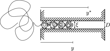
Figure 1: Schematic representation of a long blob-like polymer chain under confinement. The chain is confined up to a distance $y$, adopting a configuration of $M$ stacked blobs of size $\xi$. For a linear chain, the size of a blob scales as $\xi\sim D$. When subject to a driving flux, $J$, the competition between the hydrodynamic drag and the entropic pressure sets a barrier to translocation, located at $y^{*}$. Once it has reached the position of the barrier the polymer is able to translocate.

We start by reviewing the scaling argument of Sakaue et al. Sakaue et al. (2005) for long, blob-like linear chains. Consider a linear polymer chain of ideal radius $R_{0}\simeq aN^{1/2}$, composed of $N$ monomers of size $a$. In equilibrium, the Flory radius of the free chain is $R\simeq aN^{3/5}$.

The size of the chain changes when it is confined in a channel of width $D<R$. As depicted in Fig. 1, the chain stretches due to the effect of confinement. For a completely confined polymer, the equilibrium length of chain, $L$, follows from the minimisation of the Flory energy

$$\frac{F}{k_{B}T}\simeq\frac{L^{2}}{R_{0}^{2}}+\frac{N^{2}a^{3}}{LD^{2}},$$ (2)

and reads,

$$L\simeq D\left(\frac{a}{D}\right)^{5/3}N\simeq D\left(\frac{R}{D}\right)^{5/3}.$$ (3)

In the de Gennes’ blob picture de Gennes (1979), the confined chain accommodates itself into $M$ blobs of uniform size $\xi$. The number of blobs then obeys the relation $M=LD^{2}/\xi^{3}.$ Within each blob the effect of confinement is unimportant. Hence, the size of the blob scales as $\xi\simeq aP^{3/5}$, where $P$ is the number of monomers in each blob. Assuming that the blobs are stacked forming a mesh, one can write, for the volume fraction,

$$\phi=\frac{Na^{3}}{LD^{2}}=\frac{Pa^{3}}{\xi^{3}},$$

from which it follows that for a linear chain, the size of the blob is comparable to the pore size, i.e.,

$$\xi\simeq D.$$ (4)

II.2 Long-chain translocation

We now consider a partly confined chain in the presence of a driving flow. For a weak driving flux, the conformation of the chain outside the channel is close to equilibrium. Hence, the translocation process is controlled by the forces acting on the confined part of the chain. This corresponds to the inside approach in the terminology of Sakaue et al. Sakaue and Raphäel (2006) and is valid as long as the length of the pore, $L_{p}$, is larger than its thickness, $D$ .

The confinement of the chain has an entropic penalty of the order of $k_{B}T$ per blob de Gennes (1979). Thus, for a chain composed of $M$ blobs which penetrates a distance $y$ into the channel, as shown in Fig. 1, there is an energy cost

$$F_{S}\simeq k_{B}T\frac{yD^{2}}{\xi^{3}}=Ak_{B}T\left(\frac{y}{D}\right),$$ (5)

where we have used eq. (4), and introduced the numerical prefactor $A$ to drop the $\simeq$ symbol. As expected, the entropic cost increases with $y$, given that a larger number of monomers are pushed into the channel.

Countering the entropic cost is the fluid flow, which tends to drag the chain further into the channel. The hydrodynamic drag per blob scales as $\eta u\xi$, where $u=J/D^{2}$ is the typical velocity in the translocation direction inside the channel. For $M$ blobs, the change in free energy corresponds to the work done by the fluid to displace the chain up to a distance equal to $y$,

$$F_{H}\simeq-\eta u\int_{0}^{y}M(y^{\prime})\xi(y^{\prime})\mathrm{d}y^{\prime}=-\frac{B\eta J}{2}\left(\frac{y}{D}\right)^{2},$$ (6)

which also increases with the penetration length, both because the dragging fluid has a larger number of blobs on which to act, and because each blob has moved further into the channel. As before, we introduce a proportionality constant, $B$.

Adding the contributions given by eqs. (5) and  (6), it is possible to write the free energy change due to confinement under flow,

$$\frac{\Delta F}{k_{B}T}(y)=F_{S}+F_{H}=Ak_{B}T\left(\frac{y}{D}\right)-\frac{B\eta J}{2}\left(\frac{y}{D}\right)^{2}.$$ (7)

The competition between the entropic and hydrodynamic terms gives an energy barrier, $\Delta F^{*}$, located at $y=y^{*}$. Differentiation of eq. (7) gives the position of the barrier,

$$y^{*}=\left(\frac{A}{B}\right)\frac{k_{B}T}{\eta J}D,$$ (8)

which can be substituted back into eq. (7) to obtain its magnitude,

$$\frac{\Delta F^{*}}{k_{B}T}=\frac{A}{2}\left(\frac{y^{*}}{D}\right)=\frac{C}{2}\frac{k_{B}T}{\eta J},$$ (9)

where $C\equiv(A/B)^{2}B.$

In order that translocation proceeds, the chain must overcome this barrier. To calculate the threshold flux we consider the probability of translocation of the chain,

$$P=\kappa_{D}\tau_{m}\exp{\left(-\frac{\Delta F^{*}}{k_{B}T}\right)},$$ (10)

where $\kappa_{D}\simeq k_{B}T/\eta D^{3}$ is a characteristic frequency and $\tau_{m}$ is the observation time of the process. We define the threshold flux by

$$P(J_{c})=P_{c},$$ (11)

where $P_{c}$ is an arbitrary threshold probability. Inverting eq. (11) leads directly to the scaling relation (1),

$$J_{c}\sim\frac{k_{B}T}{\eta}.$$

As we had anticipated, $J_{c}$ does not depend on $N$. This is because the polymer reaches the position of the barrier, $y^{*}$, before it is completely confined in the channel, i.e., the translocation is triggered when $N^{*}<N$ monomers have been pushed into the channel. To obtain the critical number of monomers, $N^{*}$, it suffices to replace $L$ by $y^{*}$ in eq. (3), from which

$$N^{*}\simeq\frac{y^{*}}{D}\left(\frac{D}{a}\right)^{5/3}\simeq\left(\frac{A}{B}\right)\left(\frac{D}{a}\right)^{5/3}\frac{k_{B}T}{\eta J},$$ (12)

where we have used eq. (8). We note that in Ref. Sakaue et al. (2005) the scaling for the threshold flux was obtained by setting $\Delta F^{*}\simeq k_{B}T$ in eq. (9). This corresponds to a free energy barrier whose height is overcome by pushing only one blob into the pore, with a corresponding number of monomers $N_{D}\equiv N^{*}(y^{*}=D)\simeq(D/a)^{5/3}$.

II.3 Short-chain translocation

The short-chain regime corresponds to the limit $L<y^{*}$, or equivalently, to $N<N^{*}$, where the chain is completely confined before overcoming the energy barrier given by eq. (9). From eqs. (8) and (12), for a given chain length, this corresponds to weak fluxes and/or wide pores. Instead of being located at $y^{*}$, the energy barrier corresponds to a penetration $y=L$, given that there is no extra cost for pushing the chain into the channel any further than its own length. In terms of the number of beads, the free energy barrier obeys $\Delta F^{*}=\Delta F(L(N))$, and follows from eq. (7),

$$\frac{\Delta F^{*}}{k_{B}T}=A\left(\frac{a}{D}\right)^{5/3}\left(1-\frac{1}{2}\frac{N}{N^{*}}\right)N,$$ (13)

where we have used eqs. (3) and (12) to write the dependence on $N$ and $N^{*}$ explicitly. According to this result, for a given constant value of the flux, the barrier can be reached more easily by decreasing the number of beads. Conversely, increasing $N$ has the effect of increasing the strength of the barrier, up to $N=N^{*}$, where one crosses over to the long-chain regime, and eq. (13) reduces to eq. (9) as expected.

The threshold flux can be calculated from the probability of translocation, which follows after combining eqs. (10) and (13). Using the criterion given by eq. (11), we obtain

$$\frac{\eta J_{c}}{k_{B}T} =2\left(\frac{A}{B}\right)\left(\frac{D}{a}\right)^{10/3}$$ (14)

$$\times\left(\frac{\left(\frac{a}{D}\right)^{5/3}N+\frac{\log(P_{c})}{A}-\frac{\log(\kappa_{D}\tau_{m})}{A}}{N^{2}}\right).$$

The scaling (14) should be valid in the range $N_{D}<N<N^{*}$, which corresponds to $D<R$ and $L<y^{*}$. In this range, the threshold flux increases monotonically with the number of monomers. This behaviour can be traced back to the $N$-dependent terms in eq. (13), where the linear term, corresponding to the entropic cost, grows faster than the hydrodynamic gain, provided that $N/N^{*}<1$.

III Numerical method

To further study the cross-over from long- to short-chain translocation discussed in Section II, we use the numerical method introduced in Ref. Usta et al. (2005). This is a hybrid scheme that couples a lattice-Boltzmann fluid Ladd (1994); Ladd and Verberg (2001) to a bead-spring model for the polymer chain. Our work is based on the original implementation of the code, susp3d, which was kindly provided by the developers. Here we present the main features of the numerical method. For a more detailed description, the reader is referred to the original papers Ladd (1994); Ladd and Verberg (2001); Usta et al. (2005).

III.1 Lattice Boltzmann Method

In the lattice-Boltzmann algorithm the fluid dynamics follows from the evolution of the particle velocity distribution function ${f_{i}}$, which is defined for a discretised velocity set $\{\vec{c}_{i}\}$. For a given velocity vector, $f_{i}$ is proportional to the average number of particles moving in the direction of $\vec{c}_{i}$.

The dynamics of $f_{i}$ is given by the lattice-Boltzmann equation,

$$f_{i}(\vec{r}+\vec{c}_{i}\Delta t,t+\Delta t)-f_{i}(\vec{r},t)=\Delta_{i}(\vec{r},t)+F^{\rm ext}_{i},$$ (15)

which is defined over a lattice composed of nodes that are joined by the link vectors $\vec{c}_{i}\Delta t$, where $\Delta t$ is the time step of the algorithm. Here we use the D3Q19 model, which consists of a cubic lattice with a set of nineteen velocity vectors in three dimensions. The lattice spacing, $\Delta x$, is uniform along the lattice axes. The model has three possible magnitudes of the velocity vectors, $\{|\vec{c}_{i}|\}=(0,1,\sqrt{2})\Delta x/\Delta t$. Accordingly, the $f_{i}$ have a corresponding weight $a_{c_{i}}$ that satisfies the condition $\sum_{i}a_{c_{i}}=1$. A suitable choice of the weights for the lattice model used here is $a_{0}=1/3$, $a_{1}=1/18$ and $a_{\sqrt{2}}=1/36$.

The dynamics expressed by eq. (15) is composed of two steps. First, the distribution function undergoes a collision step, where fluid particles exchange momentum according to the collision operator, $\Delta_{i}$, and are driven by the term $F^{\rm ext}_{i}$, which plays the role of a body force. Following this collision stage, the $f_{i}$ are propagated to neighbouring sites in a streaming step, corresponding to the left-hand side of the equation.

The mapping between the lattice-Boltzmann scheme and the hydrodynamic equations follows from the definition of the hydrodynamic variables as moments of the $f_{i}$. The local density of mass, $\rho$, momentum $\rho\vec{v}$, and the momentum flux, $\Pi$, are given by

$$\sum_{i}f_{i}=\rho,\quad\sum_{i}f_{i}\vec{c}_{i}=\rho\vec{v},\quad{\rm and}\quad\sum_{i}f_{i}\vec{c}_{i}\vec{c}_{i}=\Pi,$$ (16)

respectively.

In the absence of external forces, the system relaxes towards equilibrium through the collision stage in eq. (15). For the lattice-Boltzmann model used in this paper, this is done by defining the post-collision distribution function, $f_{i}^{*}=f_{i}+\Delta_{i}$, which can be expressed as an expansion in the fluid velocity:

$$f_{i}^{*}=a_{c_{i}}\left(\rho+\frac{\rho\vec{v}\cdot\vec{c}_{i}}{c_{s}^{2}}+\frac{(\rho\vec{v}\vec{v}+\Pi^{\rm neq,*}):(\vec{c}_{i}\vec{c}_{i}-c_{s}^{2}\mathbf{1})}{2c_{s}^{4}}\right),$$ (17)

where $c_{s}=3^{-1/2}\Delta x/\Delta t$ is the speed of sound in the model. Similarly, the forcing term, $F_{i}^{\rm ext}$, can be expanded in powers of the fluid velocity (cf. Ref. Ladd and Verberg (2001)).

The post-collisional momentum flux tensor, $\Pi^{\rm neq,*}$, describes the relaxation towards the equilibrium momentum flux tensor, $\Pi^{\rm eq}$, according to

$$\Pi^{\rm neq,*}=(1+\lambda)\bar{\Pi}^{\rm neq}+\frac{1}{3}(1+\lambda_{\nu})(\Pi^{\rm neq}:\mathbf{1})\mathbf{1},$$ (18)

where $\Pi^{\rm neq}=\Pi-\Pi^{\rm eq}$, $\Pi^{\rm eq}=\rho c_{s}^{2}+\rho\vec{v}\vec{v}$, and the bar indicates the traceless part of $\Pi^{\rm neq}$.

The parameters $\lambda$ and $\lambda_{\nu}$ characterise the relaxation timescales of the lattice-Boltzmann fluid. By performing a Chapman-Enskog expansion of eq. (15), corresponding to the limit of long length and timescales compared to the lattice spacing and the relaxation timescale of the fluid, the lattice-Boltzmann scheme leads to the continuity equation for the fluid density and the Navier-Stokes equations with second order corrections in the velocity for the fluid momentum. In this limit the parameters $\lambda$ and $\lambda_{\nu}$ map to the shear and bulk viscosities of the fluid,

$$\eta=-\rho c_{s}^{2}\Delta t\left(\frac{1}{\lambda}+\frac{1}{2}\right),$$ (19)

and

$$\eta_{\nu}=-\frac{2\rho c_{s}^{2}}{3}\Delta t\left(\frac{1}{\lambda}+\frac{1}{2}\right),$$ (20)

respectively.

Solid boundaries in the simulation box are implemented using the well-known bounce-back rules Ladd and Verberg (2001). These correspond to a reflection of any distribution function propagating to a solid node back to the fluid node it came from at the streaming stage in eq. (15). As a consequence, a stick condition for the velocity is recovered approximately halfway between the fluid node and the solid node.

III.2 Polymer chain

The linear polymer is modelled by a chain composed of $N$ beads joined by freely rotating bonds. The bonds behave like Hookean springs, with an elastic potential

$$U_{\rm el}(r)=k(r-a)^{2},$$ (21)

where $r$ is the separation between adjacent beads, $a$ is the equilibrium length of the bond and $k$ is the elastic constant of the spring.

The short-range excluded-volume interactions are modelled by a truncated DLVO potential,

$$U_{\rm DLVO}=U_{0}\frac{\exp(-\kappa_{\rm DH}r)}{r},$$ (22)

where $\kappa_{\rm DH}$ is the Debye-Hückel screening length and $U_{0}$ is an amplitude.

The position vector of the $i$-th polymer bead, $\vec{x}_{i}$, evolves in time according to

$$m\ddot{\vec{x}}_{i}=-\sum_{j\neq i}\vec{\nabla}_{ij}U+\vec{F}_{i},$$ (23)

where the summation term includes the excluded-volume interactions with all beads and the elastic interactions with neighbouring beads. The term $\vec{F}_{i}$ contains the viscous hydrodynamic force that couples the bead to the lattice-Boltzmann fluid,

$$\vec{F}_{i}=-\xi_{0}(\vec{x}_{i}-\vec{v}(\vec{x}_{i}))+\vec{F}_{i}^{\rm r}.$$ (24)

This expression includes the Stokes drag, $\xi_{0}=6\pi\eta r_{\rm H},$ with $r_{H}$ being the hydrodynamic radius of the beads, and a random force $F_{i}^{\rm r}$ that satisfies the fluctuation-dissipation relation,

$$\langle\vec{F}_{i}^{\rm r}(t)\vec{F}_{i}^{\rm r}(t^{\prime})\rangle=2k_{B}T\xi_{0}\delta(t-t^{\prime})\bf 1.$$ (25)

While the polymer beads move in continuous space, the lattice-Boltzmann fluid is only defined at the lattice nodes. In order to calculate the coupling force, $\vec{F}_{i}$, the model uses a linear interpolation scheme to estimate the fluid velocity, $\vec{v}$, at the position of the bead, $\vec{x}_{i}$. The discretisation of the lattice gives an effective hydrodynamic radius, $r_{\rm H}^{\rm eff},$ which differs from the input hydrodynamic radius, $r_{\rm H}$. Here we follow the same procedure as in Ref. Usta et al. (2005), and choose $r_{\rm H}$ in order to obtain the desired value of $r_{\rm H}^{\rm eff}$. Once the hydrodynamic force has been exerted on the monomer, momentum conservation is enforced by exerting a force of equal magnitude back onto the fluid.

III.3 Parameter Values

Our objetive is to carry out numerical simulations of polymer chains in the limit where the bead-spring model gives the blob-model behaviour presented in Section II. Such regime has been validated when the monomer size matches the blob size, $a\simeq\xi$, for linear chains, where $\xi\simeq D$ Markesteijn et al. (2009). Therefore, the bead-spring model should give the blob-limit behaviour for $a\simeq D$. On the other hand, the hydrodynamic radius of the beads, $r_{\rm H}^{\rm eff}$, is limited to small values, corresponding to the point-particle coupling between the chain and the lattice-Boltzmann fluid Ahlrichs and Dünweg (1999). With these conditions in mind, we fix the bead diameter to $2r_{\rm H}^{\rm eff}=\Delta x/2$, while $a=\Delta x$ and $D=2\Delta x$.

The remaining model parameters are chosen as follows: we work at a fixed temperature, $k_{B}T=0.1$. To prevent chain crossings the spring constant is taken as $k=300k_{B}T/\Delta x^{2}$. Parameter values for the excluded-volume potential are fixed to $U_{0}=k_{B}T\Delta x$ and $\kappa_{\rm DH}=80/\Delta x$, which ensure that inter-monomer repulsions are larger than $k_{B}T$ at distances comparable to $r_{\rm H}^{\rm eff}$. To match the hydrodynamic diameter to the effective bead diameter, we fix $r_{\rm H}=0.32\Delta x$ following the calibration procedure presented in Ref. Usta et al. (2005).

In order to resolve the hydrodynamics correctly, one needs to ensure that the distribution function relaxes on a faster timescale than the diffusive timescale of the polymer chain. This condition can be satisfied by setting the parameters in the collision operator in eq. (15) to $\lambda=-1$ and $\lambda_{\nu}=-1$. We set the fluid density to $\rho=36$, and the timestep and lattice spacing in the lattice-Boltzmann fluid to $\Delta t=1$ and $\Delta x=1$. Using these values, the dynamic viscosity in simulation units is $\eta=6$.

IV Numerical Results

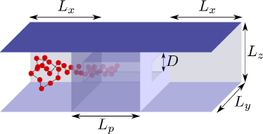
Figure 2: Schematic representation of the simulation box.

IV.1 System Geometry and Initial Conditions

The geometry of the system is depicted in Fig. 2. We consider two identical rectangular ducts of dimensions $L_{x}=108$, $L_{y}=14$ and $L_{z}=10$, separated by a square pore of width $D=2$ and length $L_{p}=24$. Solid walls are imposed in the $y$ and $z$ directions, while periodic boundary conditions are enforced in the $x$ direction.

For small Reynolds numbers, one expects that the volumetric flux, $J$, caused by applying a uniform body force to the fluid, $f$, obeys Darcy’s Law:

$$J=\frac{kS}{\eta}f,$$ (26)

where $S$ and $k$ are the local cross-sectional area and permeability of the medium and $\eta$ is the dynamic viscosity of the fluid.

In order to verify the validity of eq. (26), we measure the local flux for different applied forcings. The results, illustrated in Fig. 3, show a linear dependence of $J$ on $f$ as expected. A linear fit to the data gives $kS\simeq 238.$ For a given forcing, we find that the flux does not vary significantly whether it is measured inside or outside the pore thus confirming that, for the range of forcings considered here, the lattice-Boltzmann fluid behaves as an incompressible liquid.

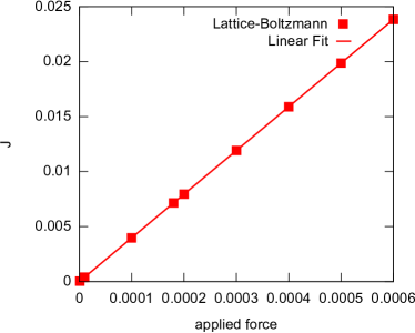
Figure 3: Volumetric flux, $J$, as a function of the body force, showing that Darcy’s law holds.

Given that we are interested in the scaling of the critical flux, we use values of the forcing that give a ratio between hydrodynamic and thermal effects in the range $0<\eta J/k_{B}T<1.5.$

We initially tether the polymer chain at a position $y=y_{0}$ inside the channel as depicted in the inset of Fig. 4, and let the system equilibrate for 5$\times$10⁴ time steps. The equilibration period allows the relaxation of the chain. Evidence for this is presented in the same figure, which shows the number of beads inside the pore, $N_{y_{0}}$, as a function of $y_{0}$ for $N=128$. For a confined chain in equilibrium, we have, from eq. (3), $N_{y_{0}}\simeq(y_{0}/D)(D/a)^{5/3}$. Our results show that the number of beads increases linearly with the tethering position, as expected.

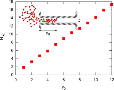
Figure 4: Number of beads in the confined part of the chain as a function of the initial tethering position. Inset: schematic representation of the tethered chain.

IV.2 Energy Barrier

In order to confirm that the polymer translocation is controlled by surpassing an energy barrier, we first perform simulations of long polymer chains subject to a fixed driving flux while varying the initial tethering position, $y_{0}$. We consider different values of $y_{0}$ in the range $0<y_{0}<L_{p}$, and set the number of monomers to $N=128$, thereby ensuring that the major part of the chain lies outside the pore.

Simulations are carried out by letting the chain equilibrate as before. Once the chain has equilibrated, it is released from its tethering point and the body force is applied uniformly to the fluid. The chain then is either carried down the pore by the underlying fluid flow and eventually translocates to the opposite duct, or is ejected from the pore back into the original chamber. Simulations are run for $5\times 10^{5}$ timesteps, which is a sufficiently long timescale to identify successful or failed translocation events.

Fig. 5 shows the probability of translocation of the chain as a function of $y_{0}$ for three different values of the imposed flux. We observe a clear transition from non-translocating ($P=0$) to translocating ($P=1$) chains as $y_{0}$ is increased. This confirms the presence of an energy barrier, which is progressively approached as the chain is pushed further into the channel. The probability curves are shifted to the left as one increases the imposed flux, $J$. This indicates a shift of the position of the barrier, $y^{*}$, closer to the pore entrance caused by a higher driving hydrodynamic force.

As a criterion we define the position of the barrier as $P(y^{*})\approx 1$, and plot the measured values of $y^{*}$ as a function of $k_{B}T/\eta J$ in the inset of Fig.  5. As expected from eq. (8), we observe a linear growth. A fit of the data shown in the figure to the function $y^{*}(x)=(A/B)Dx$ gives an estimate of the numerical prefactor in eq. (8), $A/B\simeq 4.4$.

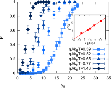
Figure 5: Probability of translocation as a function of $y_{0}$. Inset: linear growth of the position of the energy barrier with $k_{B}T/\eta J$.

The imposed flux sets the position and height of the energy barrier. Given that we fix the chain to a prescribed position inside the channel, the height of the barrier is reduced by an amount determined by $y_{0}$. This can be easily included in the analytical model by replacing $y$ by $y-y_{0}$ in eq. (5) and performing the integration in eq. (6) from $y^{\prime}=y_{0}$ to $y^{\prime}=y$. The resulting free energy barrier reads

$$\frac{\Delta F^{*}}{k_{B}T}=\frac{A}{2}\left(\frac{y^{*}}{D}\right)\left(1+g\left(\frac{y_{0}}{y^{*}}\right)\right).$$ (27)

where $g(x)\equiv-2x+x^{2}.$ From this expression and eq. (10) we can calculate the probability of translocation. This predicts $\log P\sim\Delta F^{*}/k_{B}T$ as observed in Fig. 6. As expected, all data points collapse onto the same curve, which is linear in the free energy. A fit to the data gives an estimate for the numerical prefactor in eq. (27), $A\simeq 1.8$, which together with the measured value of $A/B$, gives the amplitude of the hydrodynamic contribution to the free energy in eq. (6), $B\simeq 0.41$.

The inset in Fig. 6 shows how the theoretical prediction accurately captures the main features of the translocation process. The probability of translocation increases to unity as $y_{0}/y^{*}\rightarrow 1$. The spread of the curves is dictated by the $\sim k_{B}T/\eta J$ prefactor in eq. (27), increasing the likelihood of translocation at a given $y_{0}/y^{*}$ for larger fluxes, or lower temperatures.

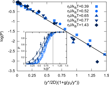
Figure 6: Logarithm of the translocation probability as a function of the free energy barrier magnitude. Symbols correspond to numerical simulations. The solid line is a linear fit to the data. Inset: translocation probability as a function of $y_{0}/y^{*}$. Numerical results (symbols) show a good agreement with the theoretical prediction (solid lines).

IV.3 Cross-over from long to short chains

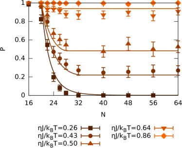
Figure 7: Probability of translocation as a function of the number of beads in the chain at different values of the imposed flux. Simulation results correspond to symbols, while the theoretical model is indicated by the solid lines where we set $N_{y_{0}}=20$ and $A=1.8$.

So far we have discussed the translocation of long chains, which can reach the position of the barrier while a significant amount of monomers remain outside the pore. The threshold flux is thus controlled only by the number of monomers that it takes to reach the barrier, $N^{*}$, and not by the total number of monomers in the chain, $N$.

This picture breaks down for shorter chains, where our theory predicts that the scaling of the critical flux becomes dependent on $N$. In order to explore this effect, we have carried out simulations at a fixed initial tethering position, $y_{0}$, and driving flux, while decreasing the total number of beads in the chain, $N$. We fix the initial tethering position to $y_{0}=L_{p}/2=12,$ for which the number of beads inside the pore after equilibration is $N_{y_{0}}\simeq 18$. We carry out the simulations in the range $16<N<64$, where we expect to observe the cross-over.

Figure 7 shows the probability of translocation as a function of $N$ for five different values of the driving flux. The probability always increases with the applied flux as expected. For large $N$ the probability is insensitive to the chain length, over a range that persists to smaller $N$ as the flux increases. For smaller $N$ the probability of translocation increases strongly with decreasing $N$ until it saturates at $N\simeq 20$ to $P\rightarrow 1$, where all polymer chains translocate even under the weakest flow.

This behaviour is in agreement with our theoretical model. For large $N$, the critical number of beads to overcome the barrier follows from eq. (12), and obeys $N^{*}\sim(D/a)^{5/3}(k_{B}T/\eta J).$ Therefore, the cross-over to the short-chain regime ($N<N^{*}$) is observed at larger chain lengths as $J$ is decreased. From eq. (12) we also have $N^{*}\sim y^{*}$, from which it is possible to estimate the critical number of beads corresponding to each driving flux by interpolating the data shown in Fig. 5. Once each value of $N^{*}$ is known, we can determine the energy barrier as a function of $N$ from eq. (13). In order to include the effect of $y_{0}$, we follow the same procedure as that used to obtain eq. (27). This gives

$$\frac{\Delta F^{*}}{k_{B}T}=A\left(\frac{a}{D}\right)^{5/3}\left[N\left(1-\frac{1}{2}\frac{N}{N^{*}}\right)+\frac{1}{2}N^{*}g\left(\frac{N_{y_{0}}}{N^{*}}\right)\right].$$ (28)

Using this expression for the free energy barrier an estimate for the probability of translocation follows from eq. (10). The observed saturation length $N\simeq 20$ is indeed in good agreement with our estimate $N_{y_{0}}\simeq 18$, at which the free energy barrier given by eq. (28) vanishes. As shown in Fig. 7, we obtain a good agreement between the theory and simulations.

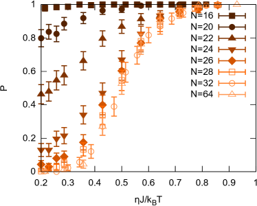
Figure 8: Probability of translocation as a function of the imposed flux for different number of monomers in the chain.

IV.4 Critical flux for small chains

We now turn our attention to the dependence of the critical flux, $J_{c}$, on the number of monomers in the short-chain regime. To find the threshold flux, we carry out simulations of the translocation process at a fixed number of beads while increasing the flux. We fix $y_{0}=12$ as before, and consider the range $0<\eta J/k_{B}T<1,$ for which the probability curves cross over from complete rejection of the chains to complete translocation.

Figure 8 shows the resulting probability curves. For $N>32$ the $N$-independence of the long-chain regime is recovered, as curves fall on top of each other. Our results in the long-chain regime are consistent with recent experimental studies of polymer translocation in nanochannels carried out by Béguin et at. Béguin et al. (2011). In their experiments they measure the rejection coefficient of chain translocation, which is related to the probability of translocation by ${\mathcal{R}}\sim 1-P$. Their experiments give the same smooth transition from rejection to translocation of the chains in the range $0<\eta J/k_{B}T<1$, very close to our simulation results. For $N<32$ the probability curves shift upwards and become increasingly plateau-like as the number of monomers is decreased, indicating the cross-over to the short-chain regime.

In order to quantify the cross-over from the short- to the long-chain regime, we use the criterion given by eq. (11) to interpolate $J_{c}$ from each of the curves shown in Fig. 8. The threshold flux is shown in Fig. 9 as a function of $N$ for six different values of the threshold probability. As expected, the overall behaviour does not depend on the particular choice of $P_{c}$. The threshold flux saturates for large $N$, corresponding to the long-chain regime, and shows a marked decrease as $N\rightarrow N_{y_{0}}$, where the chain becomes completely confined inside the channel.

Using eqs. (10), (11) and (28), we can estimate the threshold flux as a function of the number of monomers in the chain,

$$\frac{\eta J_{c}}{k_{B}T} \simeq 2\frac{A}{B}\left(\frac{D}{a}\right)^{10/3}$$ (29)

$$\times\left(\frac{\left(\frac{a}{D}\right)^{5/3}(N-N_{y_{0}})+\frac{\log(P_{c})}{A}-\frac{\log(\kappa_{D}\tau_{m})}{A}}{N^{2}-N_{y_{0}}^{2}}\right).$$

Both prefactors, $A$ and $B$, depend on the intrinsic properties of the chain and not on the particular translocation regime. We therefore set them to the values that we have measured previously.

Figure 9 shows the resulting comparison between theory and simulation. Remarkably, we find a good quantitative agreement by using no new fit parameters in our theoretical prediction.

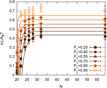
Figure 9: Threshold flux as a function of the number of monomers in the chain. $P_{c}$ is the choice of threshold probability. Simulation results: symbols. Theoretical prediction: solid lines.

V Summary and Discussion

The results presented in this paper show that the translocation of polymer chains through narrow pores exhibits two different regimes depending on the length of the chain. As previously proposed in Ref. Sakaue et al. (2005), our numerical results show that the translocation process is controlled by overcoming a free energy barrier characterised by a critical penetration of the polymer inside the pore, $y^{*}$. For long chains, this length scale always outruns the polymer length under confinement, $L$. Thus, the translocation process is controlled by $y^{*}$, regardless of the number of monomers in the chain, $N$. Conversely, for small chains, where the confined length of the polymer is smaller than $y^{*}$, we have shown that the translocation process is controlled by $L$, and the process becomes $N$-dependent. A qualitatively similar conclusion should apply to the passage of the chains through two dimensional narrow slits Sakaue (2006).

For even smaller chains, where $L$ is comparable to the size of the pore, $D$, and for very small fluxes ($\eta J/k_{B}T\simeq 10^{-1}$), we have observed a reduction of the probability of translocation of the chains. This is caused by the effect of diffusion of the chain inside the pore, which can favour the ejection of small chains at very low forcings. However, this regime falls out of the free energy barrier picture presented in this paper, and we therefore leave it for future exploration.

An application of the dependence of the translocation probability of short chains on $N$ is the potential sorting of the chains according to their number of monomers. In the short-chain regime the polymer must be completely pushed in before translocating through the pore. Given that only a small number of blobs can be pushed into the pore by fluctuations, one expects that only very short chains translocate by virtue of thermal effects in this regime. For longer chains, but still in the short-chain regime, the translocation must be assisted, for example, by a molecular motor that is able to push the chain deeper into the pore.

In an aqueous solution at room temperature, the critical flux in the long chain regime follows the scaling of eq. (1) and is of order $J_{c}\sim 10^{-18}~{}{\rm m^{3}~{}s^{-1}}$. For a micrometre sized channel the corresponding velocity, $v_{c}\simeq J_{c}/D^{2}$, is of order $10^{-6}~{}{\rm m~{}s^{-1}}$. Such a small value suggests that chains can easily translocate through microfluidic chambers at normal operation velocities, which are typically of centimetres to metres per second. However, recent experimental measurements of cytoplasmic streaming in micrometre cell channels van de Meent et al. (2009) show that the streaming velocities are in the range of $10~{}{\rm\mu m~{}s^{-1}}.$ For weaker fluxes than $J_{c}$, one enters the short-chain translocation regime. Therefore, it is feasible that the translocation regime proposed in this paper might be at play in biological systems as a regulator of selective translocation.

Here we have considered polymers in a good solvent using the DLVO potential to implement short-ranged excluded-volume interactions with the wall. Understanding the details of electrostatic effects, with regards both to the interaction with the wall and the interactions between segments, and how they are affected by the salt concentration, is an important issue for future work, relevant, in particular, to the dynamics of DNA in practical applications.

Finally, we comment on the feasibility of an experimental confirmation of our prediction. Béguin et at. Béguin et al. (2011) have recently performed an experimental study of the flow-driven translocation of hydrosoluble polymers into nanopores. In their experiments, they consider chains whose radius of gyration is $R\approx 84$ nm, and which are forced across pores $23-35$ nm in radius and $6.5~{}\mu$m in length. Their results for the rejection coefficient, $\mathcal{R}=1-\exp{\left(\Delta F^{*}/k_{B}T\right)},$ show a good agreement with the long-chain limit of the de Gennes model, where they use a similar expression to eq. (9). According to our prediction, the short chain regime would be observable for chains whose length under confinement is smaller than the position of the barrier. This traduces into a cross-over radius of gyration $R^{*}\simeq D(k_{B}T/\eta J)^{3/5}$. Taking $D=70~{}$nm and $\eta J/k_{B}T\approx 0.8$, which correspond to experimental conditions reported in ref. Béguin et al. (2011), we estimate $R^{*}\approx 80~{}$nm, which is close to the radius of gyration of the polymers used in the experiments. This supports the feasibility of future experimental work to verify the theoretical predictions presented in this paper.

VI Acknowledgements

We kindly thank Berk Usta and Tony Ladd for providing us with a copy of the numerical code. RL-A wishes to thank A. Chauduri for useful discussions. RL-A and JMY acknowledge support from EPSRC Grant EP/D050952/1.

References

- Alberts et al. (1994) B. Alberts, D. Bray, J. Lewis, M. Raff, K. Roberts and J. Watson, Molecular Biology of the Cell, Garland Publishing, New York, 1994.
- Branton et al. (2008) D. Branton, D. W. Deamer, A. Marziali, H. Bayley, S. A. Benner, T. Butler, M. Di Ventra, S. Garaj, A. Hibbs, X. Huang, S. B. Jovanovich, P. S. Krstic, S. Lindsay, X. S. Ling, C. H. Mastrangelo, A. Meller, J. S. Oliver, Y. V. Pershin, J. M. Ramsey, R. Riehn, G. V. Soni, V. Tabard-Cossa, M. Wanunu, M. Wiggin and J. A. Schloss, Nat. Biotechnol., 2008, 26, 1146–53.
- Han and Craighead (2000) J. Han and H. G. Craighead, Science, 2000, 288, 1026–1029.
- van Rijn et al. (1998) C. J. M. van Rijn, G. J. Veldhuis and S. Kuiper, Nanotechnology, 1998, 9, 343.
- Sakaue et al. (2005) T. Sakaue, E. Raphäel, P.-G. de Gennes and F. Brochard-Wyart, Eur. Phys. Lett., 2005, 72, 83.
- Sakaue and Raphäel (2006) T. Sakaue and E. Raphäel, Macromol., 2006, 39, 2621.
- Markesteijn et al. (2009) A. P. Markesteijn, O. B. Usta, I. Ali, A. C. Balazs and J. M. Yeomans, Soft Matter, 2009, 5, 4575.
- Ahlrichs and Dünweg (1999) P. Ahlrichs and B. Dünweg, J. Chem. Phys., 1999, 111, 8225.
- Usta et al. (2005) O. B. Usta, A. J. C. Ladd and J. E. Butler, J. Chem. Phys., 2005, 122, 094902.
- Usta et al. (2006) O. B. Usta, E. Butler and A. J. C. Ladd, Phys. Fluids, 2006, 18, 031703.
- Usta et al. (2007) O. B. Usta, E. Butler and A. J. C. Ladd, Phys. Rev. Lett., 2007, 98, 098301.
- de Gennes (1979) P.-G. de Gennes, Scaling Concepts in Polymer Physics, Cornell University Press, Ithaca, 1979.
- Ladd (1994) A. J. C. Ladd, Journal of Fluid Mechanics, 1994, 271, 285–309.
- Ladd and Verberg (2001) A. C. J. Ladd and R. Verberg, J. Stat. Phys., 2001, 104, 1191–1251.
- Béguin et al. (2011) L. Béguin, B. Grassi, F. Brochard-Wyart, M. Rakib and H. Duval, Soft Matter, 2011, 7, 96.
- Sakaue (2006) T. Sakaue, Euro. Phys. J. E, 2006, 19, 477–487.
- van de Meent et al. (2009) J.-W. van de Meent, A. J. Sederman, L. F. Gladden and R. E. Goldstein, J. Fluid. Mech., 2009, 642 1, 5–14.