Consistent estimation of a mean planar curve modulo similarities

Abstract

We consider the problem of estimating a mean planar curve from a set of $J$ random planar curves observed on a $k$-points deterministic design. We study the consistency of a smoothed Procrustean mean curve when the observations obey a deformable model including some nuisance parameters such as random translations, rotations and scaling. The main contribution of the paper is to analyze the influence of the dimension $k$ of the data and of the number $J$ of observed configurations on the convergence of the smoothed Procrustean estimator to the mean curve of the model. Some numerical experiments illustrate these results.

Keywords : Shape spaces; Perturbation models; Consistency; Procrustes Means; Nonparametric inference; High-dimensional data; Linear smoothing.

AMS classifications: Primary 62G08; secondary 62H11.

Acknowledgements

The authors acknowledge the support of the French Agence Nationale de la Recherche (ANR) under reference ANR-JCJC-SIMI1 DEMOS.

1 Introduction

In this paper, we are interested in the statistical treatment of random planar curves observed through rigid deformations of the plane. In many fields of interest, such data appear as, for instance, contours extracted from digital images or level sets of a real function defined on the plane. In handwriting recognition problems one typically compares curves that describe letters, digits or signatures and the acquisition process often create some ambiguity of location, size and orientation. Our aim is then to study an estimation procedure for a mean curve from a sample of $J$ noisy and discretized planar curves observed through translation, rotations and scaling. The group generated by this set of transformations is usually called similarity group of the plane and in the sequel, an element of this group will be called a deformation.

1.1 A deformable model coming from statistical shape analysis

Deformable model

In many practical cases of interest, data are collected through a computer device such as a digital camera or an image scanner. In order to take this into account in our model, we assume that observations at hand are discretized versions of continuous planar curves. Each observation $\mathbf{Y}$ is then given by a set of $k$ points of the plane called a configuration. It can be written as a $k\times 2$ real matrix

$$\mathbf{Y}=\begin{pmatrix}Y_{1}\\ \vdots\\ Y_{k}\end{pmatrix}\in\mathbb{R}^{k\times 2},$$

where $Y^{\vphantom{(1)}}_{\ell}=\big{(}Y^{(1)}_{\ell},Y_{\ell}^{(2)}\big{)}\in\mathbb{R}^{2}$ with $\ell=1,\ldots,k$. A degenerated configuration is a configuration composed of $k$ times the same point $b=(b^{(1)},b^{(2)})\in\mathbb{R}^{2}$. In tensorial notation, such a configuration is written $\mathds{1}_{k}\otimes b\in\mathbb{R}^{k\times 2}$ where $\mathds{1}_{k}$ denotes the (column) vector of $\mathbb{R}^{k}$ with all entries equal to one and $\otimes$ denotes the tensor product. From now on, we assume that the observations satisfy the following functional regression model for $j=1,\ldots,J$,

$$\mathbf{Y}_{j}=e^{a_{j}^{*}}(\boldsymbol{f}\vphantom{f}+\boldsymbol{\zeta}_{j})R_{\alpha_{j}^{*}}+\mathds{1}_{k}\otimes b_{j}^{*},\quad\mbox{ with }R_{\alpha_{j}^{*}}=\begin{pmatrix}\cos(\alpha_{j}^{*})&-\sin(\alpha_{j}^{*})\\ \sin(\alpha_{j}^{*})&\cos(\alpha_{j}^{*})\end{pmatrix},$$ (1.1)

where the unknown mean pattern $\boldsymbol{f}\vphantom{f}\in\mathbb{R}^{k\times 2}$ has been obtained by sampling on an equi-spaced design a planar curve $f=(f^{(1)},f^{(2)}):[0,1]\longrightarrow\mathbb{R}^{2}$ satisfying $f(0)=f(1)$. It means that we have

$$\boldsymbol{f}\vphantom{f}=\big{(}f(\tfrac{\ell}{k})\big{)}_{\ell=1}^{k}:=\big{(}f^{(1)}(\tfrac{\ell}{k}),f^{(2)}(\tfrac{\ell}{k})\big{)}_{\ell=1}^{k}\in\mathbb{R}^{k\times 2}.$$

The error terms $\boldsymbol{\zeta}_{j}\in\mathbb{R}^{k\times 2},\ j=1,\ldots,J$ are independent copies of a random perturbation $\boldsymbol{\zeta}$ in $\mathbb{R}^{k\times 2}$ with zero expectation. For $j=1,\ldots,J$, the scaling, rotation and translation parameters $(a_{j}^{*},\alpha_{j}^{*},b_{j}^{*})\in\mathbb{R}\times[-\pi,\pi[\times\mathbb{R}^{2}$ are independent and identically distributed (i.i.d) random variables independent of the random perturbations $\boldsymbol{\zeta}_{j}$.

Model (1.1) is a deformable model in the sens of [Bigot & Charlier, 2011] and our aim is to estimate the underlying mean curve $f:[0,1]\longrightarrow\mathbb{R}^{2}$ from $\mathbf{Y}_{1},\ldots,\mathbf{Y}_{J}\in\mathbb{R}^{k\times 2}$. More precisely, we study the influence on the estimation procedure of the number $J$ of configurations at hand and the number $k$ of discretization points composing the configurations $\mathbf{Y}_{j}$’s. Note that the model (1.1) has been introduced by Goodall in [Goodall, 1991] but with a fixed number $k$ of points in each configuration and non-random nuisance parameters $(a^{*}_{j},\alpha^{*}_{j},b^{*}_{j})$’s. This framework has been highly popular in the statistical shape community, see [Kent & Mardia, 1997, Le, 1998, Lele, 1993]. Note that the configuration $\boldsymbol{f}\vphantom{f}$ was called a population mean in [Goodall, 1991] or a perturbation mean in [Huckemann, 2011].

Shape of a configuration.

Since the seminal work of Kendall [Kendall, 1984], one considers that the shape of a configuration $\mathbf{Y}\in\mathbb{R}^{k\times 2}$ is “what remains when translations, rotations and scaling are filtered out”. More precisely, two configurations $\mathbf{Y}_{1},\mathbf{Y}_{2}\in\mathbb{R}^{k\times 2}$ are said to have the same shape if there exists a vector $(a,\alpha,b)\in\mathbb{R}\times[-\pi,\pi[\times\mathbb{R}^{2}$ such that

$$\mathbf{Y}_{2}=e^{a}\mathbf{Y}_{1}R_{\alpha}+\mathds{1}_{k}\otimes b,\quad\mbox{ with }R_{\alpha}=\begin{pmatrix}\cos(\alpha)&-\sin(\alpha)\\ \sin(\alpha)&\hphantom{-}\cos(\alpha)\end{pmatrix},$$ (1.2)

The Kendall’s Shape Space is the quotient space modulo this equivalent relation. It is usually denoted by $\boldsymbol{\Sigma}_{2}^{k}$ and defined as the set of normalized (i.e. centered and scaled to size one) configurations quotiented by the rotation of the plane, see part 2.2 for further details.

The above definition can be trivially extended to the case of planar curves by replacing the configuration $\boldsymbol{f}\vphantom{f}\in\mathbb{R}^{k\times 2}$ by the planar curve $f:[0,1]\longrightarrow\mathbb{R}^{2}$. Thence, we call shape of $f$ the set of planar curves that can be written $e^{a}fR_{\alpha}+\mathds{1}\otimes b$ for some $(a,\alpha,b)\in\mathbb{R}\times[-\pi,\pi[\times\mathbb{R}^{2}$.

1.2 Estimation of the mean curve and of the shape of the mean curve

Consistency in the Shape Space.

In shape analysis, an important issue is the computation of a sample mean shape from a set of $J$ random planar configurations $\mathbf{Y}_{1},\ldots,\mathbf{Y}_{J}\in\mathbb{R}^{k\times 2}$ satisfying model (1.1) and the study of its consistency as the number of samples $J$ goes to infinity ($k$ remaining fixed). According to Goodall [Goodall, 1991] a sample mean pattern $\hat{\boldsymbol{f}}\vphantom{f}\in\mathbb{R}^{k\times 2}$ computed from $\mathbf{Y}_{1},\ldots,\mathbf{Y}_{J}$ is said to be consistent if, as $J\to\infty$, it has asymptotically the same shape than the mean pattern $\boldsymbol{f}\vphantom{f}$. In this framework, the deformations parameters are considered as nuisance parameters that contain no informations. That is why the data are first normalized (i.e. centered and scale to unit size) without changes in the statistical analysis. The study of consistent procedures to estimate the shape of the mean pattern $\boldsymbol{f}\vphantom{f}$ using this approach has been considered by various authors [Kent & Mardia, 1997, Le, 1998, Lele, 1993, Huckemann, 2011]. In this setting, sample mean patterns obtained by a Procrustes procedure have received a special attention. In particular, it is shown in [Kent & Mardia, 1997, Le, 1998] that, in the very specific case of isotropic perturbations $\boldsymbol{\zeta}$, the so-called full and partial Procrustes sample means are consistent estimators of the shape of $\boldsymbol{f}\vphantom{f}$. Nevertheless, these estimators can be inconsistent for non-isotropic perturbations. Therefore, it is generally the belief that consistent statistical inference based on Procrustes analysis is restricted to very limited assumptions on the distribution of the data, see also [Dryden & Mardia, 1998, Kendall et al., 1999, Huckemann, 2011] for further discussions.

Estimation of the mean curve.

Our approach differ from the one developed in Shape analysis in two main aspects. First, we assume that the unknown mean pattern $\boldsymbol{f}\vphantom{f}\in\mathbb{R}^{k\times 2}$ in model (1.1) has been obtained by sampling a planar curve $f:[0,1]\longrightarrow\mathbb{R}^{2}$ on an equi-spaced design. This allows us to study the influence of the number $k$ of points composing each configuration on the estimation of $f$. Note that if $f$ is sufficently regular and $k$ is large, to estimate $\boldsymbol{f}\vphantom{f}\in\mathbb{R}^{k\times 2}$ (i.e. the values of $f$ on the design) roughly amounts to estimate $f$. The second difference concerns the randomness of the deformation parameters $(a^{*}_{j},\alpha^{*}_{j},b^{*}_{j})\in\mathbb{R}\times[-\pi,\pi[\times\mathbb{R}^{2}$, $j=1,\ldots,J$, that we want to estimate rather than to consider as nuisance parameters. Indeed, the values of the deformations parameters can be informative in some cases : assume that the size of the data are very similar except for one. This difference in size may be due to a (possibly) relevant factor and if the data are normalized as in Shape analysis this information is lost.

Under a suitable smoothness assumption on $f$, we are able to estimate consistently, with an asymptotic in $k$ only, the curve $f_{j}:=e^{a_{j}^{*}}fR_{\alpha_{j}^{*}}+\mathds{1}\otimes b_{j}^{*}$ from $\mathbf{Y}_{j}$ for each $j=1,\dots,J$. Note that, by definition, the $f_{j}$’s have the same shape as $f$. When $J$ is fixed, this smoothing step allows us to estimate consistently the deformations parameters $(a^{*}_{j},\alpha_{j}^{*},b_{j}^{*})_{j=1}^{J}$ with a Procrustes matching step. Now, if we assume that the deformations parameters $(a^{*}_{j},\alpha_{j}^{*},b_{j}^{*})$ are centered random variables, we show that it is possible to recover the true mean shape $f$ when $\min\{J,k\}\to\infty$. These results are rigorously stated in the next section, see Theorem 1.1 below.

1.3 Main contribution

Our estimating procedure is composed of two steps. First, we perform a dimension reduction step by projecting the data into a low-dimensional space of $\mathbb{R}^{k\times 2}$ to eliminate the influence of the random perturbations $\boldsymbol{\zeta}_{j}$. Then, in a second step, we apply Procrustes analysis in this low-dimensional space to obtain a consistent estimator of $\boldsymbol{f}\vphantom{f}\in\mathbb{R}^{k\times 2}$.

The reduction dimension step is based on an appropriate smoothness assumptions on $f$. Let $L>0$, $s>0$ and define the Sobolev ball of radius $L$ and degree $s$ as

$$H_{s}(L)=\Big{\{}f=(f^{(1)},f^{(2)})\in L^{2}([0,1],\mathbb{R}^{2}),\ \sum_{m\in\mathbb{Z}}(1+\lvert m\rvert^{2})^{s}(\lvert c_{m}(f^{(1)})\rvert^{2}+\lvert c_{m}(f^{(2)})\rvert^{2})<L\ )\Big{\}}$$ (1.3)

where $c_{m}(f)=(c_{m}(f^{(1)}),c_{m}(f^{(2)}))=\Big{(}\int_{0}^{1}f^{(1)}(t)e^{-i2\pi mt}dt,\int_{0}^{1}f^{(2)}(t)e^{-i2\pi mt}dt\Big{)}\in\mathbb{C}^{2}$ is the $m$-th Fourier coefficient of $f=(f^{(1)},f^{(2)})\in L^{2}([0,1],\mathbb{R}^{2})$, for $m\in\mathbb{Z}$.

Assumption 1.

The curve $f:[0,1]\longrightarrow\mathbb{R}^{2}$ is closed, i.e. $f(0)=f(1)\in\mathbb{R}^{2}$, and belongs to $H_{s}(L)$ for some $L>0$ and $s>\frac{3}{2}$. Moreover, the $k\times 2$ matrix $\boldsymbol{f}\vphantom{f}=\big{(}f(\tfrac{\ell}{k})\big{)}_{\ell=1}^{k}$ is of rank two, i.e. the configuration $\boldsymbol{f}\vphantom{f}$ is not degenerated.

Assumption 1 implies that $f$ is not reduced to a point, continuously differentiable and is equal to its Fourier series. We introduce the following $k\times k$ matrix

$$\mathbf{A}^{\lambda}=\bigg{(}\frac{1}{k}\sum_{0\leq|m|\leq\lambda}e^{i2\pi m\tfrac{\ell-\ell^{\prime}}{k}}\bigg{)}_{\ell,\ell^{\prime}=1}^{k}.$$ (1.4)

The matrix $\mathbf{A}^{\lambda}$ is the smoothing matrix corresponding to a discrete Fourier low pass filter with frequency cutoff $\lambda\in\mathbb{N}$. It is a projection matrix in a sub-space $\boldsymbol{\mathcal{V}}^{\lambda}$ of $\mathbb{R}^{k}$ of dimension $2\lambda+1$. Then, we project the data on $\boldsymbol{\mathcal{V}}^{\lambda}\times\boldsymbol{\mathcal{V}}^{\lambda}\subset\mathbb{R}^{k\times 2}$, and we estimate the scaling, rotation and translation parameters in model (1.1) using M-estimation as follows: denote the scaling parameters by $\boldsymbol{a}=(a_{1},\ldots,a_{J})\in\mathbb{R}^{J}$, the rotation parameters by $\boldsymbol{\alpha}=(\alpha_{1},\ldots,\alpha_{J})\in\mathbb{R}^{J}$ and the translation parameters by $\boldsymbol{b}\vphantom{b}=(b_{1},\ldots,b_{J})\in\mathbb{R}^{2J}$, and introduce the functional,

$$M^{\lambda}(\boldsymbol{a},\boldsymbol{\alpha},\boldsymbol{b}\vphantom{b})=\frac{1}{Jk}\sum_{j=1}^{J}\bigg{\|}e^{-a_{j}}\mathbf{A}^{\lambda}(\mathbf{Y}_{j}-\mathds{1}_{k}\otimes b_{j})R_{-\alpha_{j}}-\frac{1}{J}\sum_{j^{\prime}=1}^{J}e^{-a_{j^{\prime}}}\mathbf{A}^{\lambda}(\mathbf{Y}_{j^{\prime}}-\mathds{1}_{k}\otimes b_{j^{\prime}})R_{-\alpha_{j^{\prime}}}\bigg{\|}^{2}_{\mathbb{R}^{k\times 2}},$$ (1.5)

where $\lVert\cdot\rVert_{\mathbb{R}^{k\times 2}}$ is the standard Euclidean norm in $\mathbb{R}^{k\times 2}$. An M-estimator of

$$\big{(}\boldsymbol{a}^{*},\boldsymbol{\alpha}^{*},\boldsymbol{b}\vphantom{b}^{*}\big{)}=\big{(}a^{*}_{1},\ldots,a^{*}_{J},\alpha^{*}_{1},\ldots,\alpha^{*}_{J},b^{*}_{1},\ldots,b^{*}_{J}\big{)}\in\mathbb{R}^{J}\times[-\pi,\pi[^{J}\times\mathbb{R}^{2J}$$

is given by

$$(\hat{}\boldsymbol{a}^{\lambda},\hat{}\boldsymbol{\alpha}^{\lambda},\hat{}\boldsymbol{b}\vphantom{b}\vphantom{\boldsymbol{b}\vphantom{b}}^{\lambda})\in\operatorname*{\mbox{argmin}}_{(\boldsymbol{a},\boldsymbol{\alpha},\boldsymbol{b}\vphantom{b})\in\boldsymbol{\Theta}_{0}}M^{\lambda}(\boldsymbol{a},\boldsymbol{\alpha},\boldsymbol{b}\vphantom{b}),$$ (1.6)

where $\big{(}\hat{}\boldsymbol{a}^{\lambda},\hat{}\boldsymbol{\alpha}^{\lambda},\hat{}\boldsymbol{b}\vphantom{b}\vphantom{\boldsymbol{b}\vphantom{b}}^{\lambda}\big{)}=\big{(}\hat{a}^{\lambda}_{1},\ldots,\hat{a}^{\lambda}_{J},\hat{\alpha}^{\lambda}_{1},\ldots,\hat{\alpha}^{\lambda}_{J},\hat{b}\vphantom{\boldsymbol{b}\vphantom{b}}^{\lambda}_{1},\ldots,\hat{b}\vphantom{\boldsymbol{b}\vphantom{b}}^{\lambda}_{J}\big{)}\in\mathbb{R}^{J}\times[-\pi,\pi[^{J}\times\mathbb{R}^{2J}$ and

$$\boldsymbol{\Theta}_{0}=\bigg{\{}(\boldsymbol{a},\boldsymbol{\alpha},\boldsymbol{b}\vphantom{b})\in[-A,A]^{J}\times[-\mathcal{A},\mathcal{A}]^{J}\times\mathbb{R}^{2J}:\sum_{j=1}^{J}a_{j}=0,\ \sum_{j=1}^{J}\alpha_{j}=0\mbox{ and }\sum_{j=1}^{J}b_{j}=0\bigg{\}},$$ (1.7)

with $A,\mathcal{A}>0$ being parameters whose values will be discussed below.

Finally, the mean pattern $\boldsymbol{f}\vphantom{f}$ is estimated by the following smoothed Procrustes mean

$$\hat{\boldsymbol{f}}\vphantom{f}\vphantom{\boldsymbol{f}\vphantom{f}}^{\lambda}=\frac{1}{J}\sum_{j=1}^{J}e^{-\hat{a}^{\lambda}_{j}}\left(\mathbf{A}^{\lambda}\mathbf{Y}_{j}-\mathds{1}_{k}\otimes\hat{b}_{j}^{\lambda}\right)R_{-\hat{\alpha}_{j}^{\lambda}}.$$ (1.8)

To analyze the convergence of the estimator $\hat{\boldsymbol{f}}\vphantom{f}\vphantom{\boldsymbol{f}\vphantom{f}}^{\lambda}$ to the mean pattern $\boldsymbol{f}\vphantom{f}$, let us introduce some regularity conditions on the covariance structure of the random variable $\boldsymbol{\zeta}$ in $\mathbb{R}^{k\times 2}$. Let $\tilde{}\boldsymbol{\zeta}=(\boldsymbol{\zeta}^{(1)},\boldsymbol{\zeta}^{(2)})=(\zeta^{(1)}_{1},\ldots,\zeta_{k}^{(1)},\zeta^{(2)}_{1},\ldots,\zeta^{(2)}_{k})\in\mathbb{R}^{2k}$ be the vectorized version of $\boldsymbol{\zeta}=(\zeta^{(1)}_{\ell},\linebreak[1]\zeta^{(2)}_{\ell})_{\ell=1}^{k}\in\mathbb{R}^{k\times 2}$.

Assumption 2.

The random variable $\tilde{}\boldsymbol{\zeta}$ is a centered Gaussian vector in $\mathbb{R}^{2k}$ with covariance matrix $\boldsymbol{\Sigma}_{k}\in\mathbb{R}^{2k\times 2k}$. Let $\gamma_{\max}(k)$ be the largest eigenvalue of $\boldsymbol{\Sigma}_{k}$. Then,

$$\lim_{k\to\infty}\gamma_{\max}(k)k^{-\frac{2s}{2s+1}}=0,$$

where $s$ is the smoothness parameter defined in Assumption 1.

For example, the isotropic Gaussian error model corresponds to $\boldsymbol{\Sigma}_{k}=Id_{k}$ and $\gamma_{\max}(k)=1$ satisfies Assumption 2. If there exists correlations terms (i.e. non-zero off-diagonal entries in $\boldsymbol{\Sigma}_{k}$), then the level of the perturbation $\tilde{}\boldsymbol{\zeta}$ has to be sufficiently small. A simple model is the case where $\boldsymbol{\Sigma}_{k}=\left[S(\left\lvert\ell-\ell^{\prime}\right\rvert)\right]_{\ell,\ell^{\prime}=1}^{k}$ for some function $S:\mathbb{R}\longrightarrow\mathbb{R}$ satisfying $\int_{\mathbb{R}}\left\lvert S(t)\right\rvert dt<+\infty$ implying that $\gamma_{\max}(k)\leq\sum_{\ell\in\mathbb{Z}}|S(\ell)|$ (see Lemma 4.11 in [Gray, 2006]) and thus Assumption 2 is again satisfied. The following theorem is the main result of the paper.

Theorem 1.1.

Consider model (1.1) and suppose that Assumptions 1 and 2 hold. Suppose also that the random variables $(\boldsymbol{a}^{*},\boldsymbol{\alpha}^{*},\boldsymbol{b}\vphantom{b}^{*})$ are bounded and belong to $[-\tfrac{A}{2},\tfrac{A}{2}]^{J}\times[-\tfrac{\mathcal{A}}{2},\tfrac{\mathcal{A}}{2}]^{J}\times[-B,B]^{2J}$ for some $0<A,B$ and $0<\mathcal{A}<\frac{\pi}{4}$ and that $\lambda(k)=k^{\frac{1}{2s+1}}$.

• For any $J\geq 2$ there exists $\boldsymbol{f}\vphantom{f}_{\boldsymbol{\Theta}_{0}}=e^{a_{0}}\boldsymbol{f}\vphantom{f}R_{\alpha_{0}}+\mathds{1}_{k}\otimes b_{0}$ for some $(a_{0},\alpha_{0},b_{0})\in\mathbb{R}\times[-\pi,\pi[\times\mathbb{R}^{2}$ and a function $V_{1}(k,x)$ such that for any $x>0$,

  $$\mathbb{P}\left(\frac{1}{k}\lVert\hat{\boldsymbol{f}}\vphantom{f}\vphantom{\boldsymbol{f}\vphantom{f}}^{\lambda}-\boldsymbol{f}\vphantom{f}_{\boldsymbol{\Theta}_{0}}\rVert^{2}_{\mathbb{R}^{k\times 2}}\geq V_{1}(k,x)\right)\leq e^{-x},$$ (1.9)

  with $V_{1}(k,x)\to 0$ when $k\to\infty$ and $x$ remains fixed.

• Suppose, in addition, that the random variables $(\boldsymbol{a}^{*},\boldsymbol{\alpha}^{*},\boldsymbol{b}\vphantom{b}^{*})$ have zero expectation in $[-\tfrac{A}{2},\tfrac{A}{2}]^{J}\times[-\tfrac{\mathcal{A}}{2},\tfrac{\mathcal{A}}{2}]^{J}\times[-B,B]^{2J}$ with $A,\mathcal{A}<0.1$. Then, there exists a function $V_{2}(J,k,x)$ such that for any $x>0$,

  $$\mathbb{P}\left(\frac{1}{k}\lVert\hat{\boldsymbol{f}}\vphantom{f}\vphantom{\boldsymbol{f}\vphantom{f}}^{\lambda}-\boldsymbol{f}\vphantom{f}\rVert^{2}_{\mathbb{R}^{k\times 2}}\geq V_{2}(J,k,x)\right)\leq e^{-x},$$ (1.10)

  where $V_{2}(J,k,x)\to 0$ when $\min\{J,k\}\to\infty$ and $x$ remains fixed.

Statement (1.9) means that, under mild assumptions on the covariance structure of the error terms $\boldsymbol{\zeta}_{j}$, it is possible to consistently estimate the shape of the mean curve $f$ when the number of observations $J$ is fixed and the number $k$ of discretization points increases. Note that $(a_{0},\alpha_{0},b_{0})$ depends on $J$ and is given by formula (3.3) in Section 3. The function $V_{1}(k,x)$ is explicitly given in Section 5.2. To obtain statement (1.10), we assume the condition $A,\mathcal{A}<0.1$ which means that the random scaling and rotations in model (1.1) are not too large. Also, it is assumed that random scaling, rotations and translations have zero expectation, meaning that the deformations parameters in model (1.1) are centered around the identity. Then, under such assumptions, statement (1.10) shows that one can consistently estimate the true mean curve $f$ when both the sample size $J$ and the number of landmarks $k$ go to infinity. Again, the function $V_{2}(J,k,x)$ is explicitly given in Section 5.2. These results are consistent with those obtained in [Bigot & Charlier, 2011], where we have studied the consistency of Fréchet means in deformable models for signal and image processing.

1.4 Organization of the paper

In Section 2, we recall some properties on the similarity group of the plane, and we describe its action on the mean pattern $\boldsymbol{f}\vphantom{f}$. Then, we discuss General Procrustes Analysis (GPA) and we compare it to our approach. In Section 3 we discuss some identifiability issues in model (1.1). The estimating procedure is described in detail in Section 4. Consistency results are given in Section 5. Some experiments in Section 6 illustrate the numerical performances of our approach. All the proofs are gathered in a technical appendix.

2 Group structure and Generalized Procrustes Analysis

2.1 The similarity group

Group action

First let us introduce some notations and definitions that will be useful throughout the paper. The similarity group of the plane is the group $(\mathcal{G},.)$ generated by isotropic scaling, rotations and translations. The identity element in $\mathcal{G}$ is denoted $e$ and the inverse of $g\in\mathcal{G}$ is denoted by $g^{-1}$. We parametrize the group $\mathcal{G}$ by a scaling parameter $a\in\mathbb{R}$, an angle $\alpha\in[-\pi,\pi[$ and a translation $b\in\mathbb{R}^{2}$, and we make no difference between $g\in\mathcal{G}$ and its parametrization $(a,\alpha,b)\in\mathbb{R}\times[-\pi,\pi[\times\mathbb{R}^{2}$. For all $g_{1}=(a_{1},\alpha_{1},b_{1}),g_{2}=(a_{2},\alpha_{2},b_{2})\in\mathbb{R}\times[-\pi,\pi[\times\mathbb{R}^{2}$ we have

$$g_{1}.g_{2}=(a_{1},\alpha_{1},b_{1}).(a_{2},\alpha_{2},b_{2}) =(a_{1}+a_{2},\alpha_{1}+\alpha_{2},e^{a_{1}}b_{2}R_{\alpha_{1}}+b_{1}),$$

$$g_{1}^{-1}=(a_{1},\alpha_{1},b_{1})^{-1} =(-a_{1},-\alpha_{1},-e^{-a_{1}}b_{1}R_{-\alpha_{1}}),$$ (2.1)

$$e =(0,0,0).$$

The action of $\mathcal{G}$ onto $\mathbb{R}^{k\times 2}$ is given by the mapping $(g,\boldsymbol{x})\longmapsto g.\boldsymbol{x}:=e^{a}\boldsymbol{x}R_{\alpha}+\mathds{1}_{k}\otimes b,$ for $g=(a,\alpha,b)\in\mathcal{G}$ and $\boldsymbol{x}\in\mathbb{R}^{k\times 2}$. Note that we use the same symbol “.” for the composition law of $\mathcal{G}$ and its action on $\mathbb{R}^{k\times 2}$. This action can also be defined on $L^{2}([0,1],\mathbb{R}^{2})$ by replacing $\boldsymbol{f}\vphantom{f}$ by $f\in L^{2}([0,1],\mathbb{R}^{2})$. Coming back to the final dimensional case, let

$$\boldsymbol{1}_{k\times 2}=\mathds{1}_{k}\otimes\mathbb{R}^{2}$$

be the two dimensional linear subspace of $\mathbb{R}^{k\times 2}$ consisting of degenerated configurations, i.e. configurations composed of $k$ times the same landmarks. The orthogonal subspace $\boldsymbol{1}^{\perp}_{k\times 2}$ is the set of centered configurations. We have the orthogonal decomposition $\mathbb{R}^{k\times 2}=\boldsymbol{1}^{\perp}_{k\times 2}\oplus\boldsymbol{1}^{\phantom{\perp}}_{k\times 2},$ and for any configuration $\boldsymbol{x}\in\mathbb{R}^{k\times 2}$ we write $\boldsymbol{x}=\boldsymbol{x}_{0}+\bar{}\boldsymbol{x}\in\boldsymbol{1}^{\perp}_{k\times 2}\oplus\boldsymbol{1}^{\phantom{\perp}}_{k\times 2}$. We call $\boldsymbol{x}_{0}$ the centered configuration of $\boldsymbol{x}$ and $\bar{}\boldsymbol{x}=\mathds{1}_{k}\otimes\Big{(}\frac{1}{k}\sum_{\ell=1}^{k}x^{(1)}_{\ell},\frac{1}{k}\sum_{\ell=1}^{k}x^{(2)}_{\ell}\Big{)}$ the degenerated configuration associated to $\boldsymbol{x}$, see Figure 1 for an illustration.

Orbit, stabilizer and section

Given a configuration $\boldsymbol{x}$ in $\mathbb{R}^{k\times 2}$, the orbit of $\boldsymbol{x}$ is defined as the set

$$\mathcal{G}.\boldsymbol{x}:=\{g.\boldsymbol{x},\ g\in\mathcal{G}\}\subset\mathbb{R}^{k\times 2}.$$

This set is also called the shape of $\boldsymbol{x}$. The orbit of any degenerated configuration is the entire subspace $\boldsymbol{1}_{k\times 2}$. Note also that the linear subspace $\boldsymbol{1}_{k\times 2}$ is stable by the action of $\mathcal{G}$, and that the action of $\mathcal{G}$ on $\boldsymbol{1}_{k\times 2}$ is not free, meaning that for any $\bar{}\boldsymbol{x}\in\boldsymbol{1}_{k\times 2}$ the equality $g_{1}.\bar{}\boldsymbol{x}=g_{2}.\bar{}\boldsymbol{x}$ does not imply that $g_{1}=g_{2}$. Now, if $\boldsymbol{x}\in\mathbb{R}^{k\times 2}\setminus\boldsymbol{1}_{k\times 2}$ is a non-degenerated configuration of $k$ landmarks, its orbit $\mathcal{G}.\boldsymbol{x}$ is a sub-manifold of $\mathbb{R}^{k\times 2}\setminus\boldsymbol{1}_{k\times 2}$ of dimension $\dim(\mathcal{G})=4$.

Given a configuration $\boldsymbol{x}\in\mathbb{R}^{k\times 2}$, the stabilizer $I(\boldsymbol{x})$ is the closed subgroup of $\mathcal{G}$ which leaves $\boldsymbol{x}$ invariant, namely

$$I(\boldsymbol{x})=\{g\in\mathcal{G}:\ g.\boldsymbol{x}=\boldsymbol{x}\}.$$

If $\bar{}\boldsymbol{x}=\mathds{1}_{k}\otimes(\bar{x}^{(1)},\bar{x}^{(2)})\in\boldsymbol{1}_{k\times 2}$ is a degenerated configuration, its stabilizer is non trivial and is equal to $I(\bar{}\boldsymbol{x})=\{(a,\alpha,(\bar{x}^{(1)},\bar{x}^{(2)})-e^{a}(\bar{x}^{(1)},\bar{x}^{(2)})R_{\alpha}),\ a\in\mathbb{R},\ \alpha\in[-\pi,\pi[\}$. If $\boldsymbol{x}\in\mathbb{R}^{k\times 2}\setminus\boldsymbol{1}_{k\times 2}$ is a non-degenerated configuration, its stabilizer $I(\boldsymbol{x})$ is trivial, i.e. is reduced to the identity $\{e\}$. The action of $\mathcal{G}$ is said free if the stabilizer of any point is reduced to the identity. Hence, the action of $\mathcal{G}$ is free on the set of non-degenerated configurations of $k$-ads in $\mathbb{R}^{2}$.

A section of the orbits of $\mathcal{G}$ is a subset of $\mathbb{R}^{k\times 2}$ containing a unique element of each orbit. A well-known example of section for the similarity group acting on $\mathbb{R}^{k\times 2}\setminus\boldsymbol{1}_{k\times 2}$ is the so-called Bookstein’s coordinates system (see e.g. [Dryden & Mardia, 1998] p. 27).

Figure 1: Three orbits of the action of the similarity group $\mathcal{G}$ are represented in blue. The space of centered configurations $\boldsymbol{1}_{k\times 2}^{\perp}$ is the green plane. The preshape sphere $\mathbb{S}_{2}^{k}$ is the red circle. For a particular $\boldsymbol{x}\in\mathbb{R}^{k\times 2}$, the centered version is $\boldsymbol{x}_{0}$ and the centered and normalized version is $\boldsymbol{x}^{0}$. The degenerated configuration associated to $\boldsymbol{x}$ is $\bar{}\boldsymbol{x}$.

2.2 Kendall’s shape space and Generalized Procrustes analysis

Shape space

Let $\boldsymbol{x}\in\mathbb{R}^{k\times 2}\setminus\boldsymbol{1}_{k\times 2}$ be a non-degenerated configuration. Let $H=Id_{k}-\frac{1}{k}\mathds{1}_{k}\mathds{1}_{k}^{\prime}$ be a centering matrix. The effect of translation can be eliminated by centering the configuration $\boldsymbol{x}$ using the matrix $H$ (see [Dryden & Mardia, 1998] for other centering methods), while the effect of isotropic scaling is removed by projecting the centered configuration on a unit sphere, which yields to the so-called pre-shape $\boldsymbol{x}^{0}$ of $\boldsymbol{x}$ defined as

$$\boldsymbol{x}^{0}=\frac{H\boldsymbol{x}}{\|H\boldsymbol{x}\|}_{\mathbb{R}^{k\times 2}}\in\mathbb{R}^{k\times 2}.$$

Consider now the pre-shape sphere defined by $\mathbb{S}^{k}_{2}:=\left\{\boldsymbol{x}^{0},\ \boldsymbol{x}\in\mathbb{R}^{k\times 2}\setminus\boldsymbol{1}_{k\times 2}\right\}$ and see Figure 1 for an illustration. Note that this normalization of the planar configurations amounts to choose a section for the action of the group generated by the translation and scaling in the plane. The Kendall’s shape space is then defined as the quotient of $\mathbb{S}^{k}_{2}$ by the group $\mathbf{SO}(2)$ of rotations of the plane, namely

$$\boldsymbol{\Sigma}_{2}^{k}:=\mathbb{S}^{k}_{2}/\mathbf{SO}(2)=\left\{[\boldsymbol{x}^{0}]:\boldsymbol{x}^{0}\in\mathbb{S}^{k}_{2}\right\}\mbox{ with }[\boldsymbol{x}^{0}]=\left\{\boldsymbol{x}^{0}R_{\alpha},\alpha\in[-\pi,\pi[\right\}.$$

The space $\boldsymbol{\Sigma}_{2}^{k}$ can be endowed with a Riemannian structure and we refer to [Kendall et al., 1999] for a detail discussion on its geometric properties.

Let us briefly recall the definition of the so-called partial and full Procrustes distances on $\mathbb{S}^{k}_{2}$. The partial Procrustes distance is defined on the pre-shape sphere $\mathbb{S}_{2}^{k}$ as

$$d_{P}^{2}(\boldsymbol{x}^{0},\boldsymbol{y}^{0})=\inf_{\alpha\in[-\pi,\pi[}\lVert\boldsymbol{x}^{0}-\boldsymbol{y}^{0}R_{\alpha}\rVert^{2}_{\mathbb{R}^{k\times 2}},\qquad\boldsymbol{x},\boldsymbol{y}\in\mathbb{S}_{2}^{k}.$$

Hence, it is the (Euclidean) distance between the orbits $[\boldsymbol{x}^{0}]=\mathbf{SO}(2).\boldsymbol{x}^{0}$ and $[y^{0}]=\mathbf{SO}(2).\boldsymbol{y}^{0}$ with $\boldsymbol{x}^{0},\boldsymbol{y}^{0}\in\mathbb{S}_{2}^{k}$. Let now $\mathcal{H}$ be the group of transformations of the plane generated by scaling and rotations. The action of $h\in\mathcal{H}$ on the centered configuration $\boldsymbol{x}^{0}$ is defined as $h.\boldsymbol{x}^{0}:=e^{a}\boldsymbol{x}^{0}R_{\alpha}$ where $h=(a,\alpha)\in\mathbb{R}\times[-\pi,\pi[$. The Full Procrustes distance is then defined as

$$d_{F}^{2}(\boldsymbol{x}^{0},\boldsymbol{y}^{0})=\inf_{h\in\mathcal{H}}\lVert\boldsymbol{x}^{0}-h.\boldsymbol{y}^{0}\rVert^{2}_{\mathbb{R}^{k\times 2}},\qquad\boldsymbol{x},\boldsymbol{y}\in\mathbb{S}_{2}^{k}.$$

Generalized Procrustes analysis

The full Procrustes sample mean $\hat{\mathbf{Y}}_{F}$ of $\mathbf{Y}_{1},\ldots,\mathbf{Y}_{J}$ (see e.g.  [Goodall, 1991, Dryden & Mardia, 1998]) is defined by

$$\hat{\mathbf{Y}}_{F}=\operatorname*{\mbox{argmin}}_{\boldsymbol{x}^{0}\in\mathbb{S}_{2}^{k}}\sum_{j=1}^{J}d_{F}^{2}(\mathbf{Y}^{0}_{j},\boldsymbol{x}^{0}).$$ (2.2)

The partial Procrustes mean $\hat{\mathbf{Y}}_{P}$ is defined in the same way by replacing $d_{F}$ by $d_{P}$ in (2.2). Thence, this two Procrustes means are Fréchet mean either on $(\mathbb{S}^{k}_{2},d_{F})$ or $(\mathbb{S}^{k}_{2},d_{P})$ endowed with the empirical measure $\mu_{J}=\sum_{j=1}^{J}\delta_{\mathbf{Y}_{j}}$.

In practice, there are several way to compute the full Procrustes mean. In [Kent, 1992] the author used complex coordinates and expressed the full Procrustes mean as the biggest eigenvalue of a symmetrical positive definite complex matrix, see [Dryden & Mardia, 1998] result 3.2 and [Bhattacharya & Patrangenaru, 2003]. The full Procrustes mean $\hat{\mathbf{Y}}_{F}$ can also be approximated by General Procrustes procedure which amounts to use the following identity

$$\hat{\mathbf{Y}}_{F}=\frac{1}{J}\sum_{j=1}^{J}\hat{h}_{j}\cdot\mathbf{Y}_{j}^{0}$$ (2.3)

where $\hat{h}_{1},\ldots,\hat{h}_{J}$ are the argmins of the functional $M(h_{1},\ldots,h_{J})=\frac{1}{J}\sum_{j=1}^{J}\big{\|}h_{j}.\mathbf{Y}_{j}^{0}-\frac{1}{J}\sum_{j^{\prime}=1}^{J}h_{j^{\prime}}.\mathbf{Y}_{j^{\prime}}^{0}\big{\|}^{2}_{\mathbb{R}^{k\times 2}}$ subject to the constraint $\|\frac{1}{J}\sum_{j=1}^{J}h_{j}.\mathbf{Y}_{j}^{0}\|_{\mathbb{R}^{k\times 2}}^{2}=1$. The configurations $\hat{h}.\mathbf{Y}_{j}$’s are known as Full Procrustes fits and the $\hat{h}$ can be explicitly computed by using a singular value decomposition. In practice, one can use the iterative General Procrustes algorithm to compute $\hat{\mathbf{Y}}$, see [Dryden & Mardia, 1998] pages 90-91.

2.3 Discussion on the double asymptotic setting and comparison with GPA

Asymptotic settings

When random planar curves (such as digits or letters for instance) are observed, a natural framework for statistical inference is an asymptotic setting in the number $J$ of curves. This setting means that increasing the number of curves at hand should help to compute a more accurate empirical mean curve. Unfortunately, consistency results of Procrustes type procedures are reduced to the very specific case of an isotropic perturbation. In this paper, we show that increasing the number $k$ of discretization points will ensure a consistent estimation of a mean shape in more general cases.

Consider model (1.1) where $k>2$ is fixed and the random perturbation $\boldsymbol{\zeta}$ is isotropic, (see Proposition 1 in [Le, 1998] for a precise definition of isotropy for random variables belonging to $\mathbb{R}^{k\times 2}$). In this framework, it has been proved in [Kent & Mardia, 1997] that the functional $M_{J}(\boldsymbol{x}^{0})=\frac{1}{J}\sum_{j=1}^{J}d_{F}^{2}(\mathbf{Y}_{j},\boldsymbol{x}^{0})$ defined on $\mathbb{R}^{k\times 2}$ converge uniformly in probability to the functional $M(\boldsymbol{x}^{0})=\mathbb{E}(d^{2}_{F}(\mathbf{Y}_{1},\boldsymbol{x}^{0}))$ which admits a unique minimum at $[\boldsymbol{f}\vphantom{f}^{0}]$. These two facts imply that $[\hat{\mathbf{Y}}_{F}]$ converges almost surely to $[\boldsymbol{f}\vphantom{f}^{0}]$ as $J\to+\infty$. In [Le, 1998] the author used a Fréchet mean approach to show the consistency of $\hat{\mathbf{Y}}_{F}$ with a slightly more general kind of noise. Finally, note that the estimator $\hat{\mathbf{Y}}_{P}$ defined above is also studied in [Kent & Mardia, 1997, Le, 1998] with similar consistency results.

When the random perturbation $\boldsymbol{\zeta}$ in model (1.1) is non-isotropic, it has been argued in [Kent & Mardia, 1997] that the Procrustes estimator $\hat{\mathbf{Y}}_{F}$ can be arbitrarily inconsistent when the signal-to-noise ratio decrease. The heuristic presented by the authors suggests that the main phenomenon that prevent the Procrustes estimator to be consistent is the fact that the functional $M$ do not attain its minimum at $[\boldsymbol{f}\vphantom{f}^{0}]$. In section 4.2 of [Huckemann, 2011] the author makes this remark clear as he gives an explicit example : given a mean pattern $\boldsymbol{f}\vphantom{f}^{0}$, the idea is to increase the level of noise $\boldsymbol{\zeta}$ until the argmin of the functional $M$ which was initially equals to $[\boldsymbol{f}\vphantom{f}_{0}]$ jumps abruptly to another point. This phenomenon seems to be linked to the geometry of the sphere and properties of the Fréchet mean.

Comparison with GPA

Hence, it is commonly the belief that Procrustes sample means can be inconsistent when considering convergence in $\boldsymbol{\Sigma}_{2}^{k}$ and the asymptotic setting $J\to+\infty$. Nevertheless, the above discussion suggests that a sufficient condition to ensure the consistency of Procrutres type estimators is to control the level of non-isotropic noise. That is why we introduced a pre-smoothing step that takes advantage of increasing the number $k$ of points composing each configuration in order to ensure more general consistency results. Therefore, our approach and GPA share some similarities. They are both based on the estimation of scaling, rotation and translation parameters by a Procrustean procedure which leads to the M-estimators (1.6) which is related to (2.2). To compute a sample mean shape, this M-estimation step is then followed by a standard empirical mean in $\mathbb{R}^{k\times 2}$ of the aligned data using these estimated deformation parameters, see equations (1.8) and (2.3).

However, one of the main differences between the approach developed in this paper and GPA is the choice of the normalization of the data. In GPA, the deformation parameters $\hat{h}_{1},\ldots,\hat{h}_{J}$ are computed so that the full Procrustes sample mean $\hat{\mathbf{Y}}_{F}$ belongs to the pre-shape sphere $\mathbb{S}^{k}_{2}$, see the constraint appearing in (2.2). Therefore, the computation of $\hat{h}_{1},\ldots,\hat{h}_{J}$ is somewhat independent of any assumption on the true parameters $(\boldsymbol{a}^{*},\boldsymbol{\alpha}^{*},\boldsymbol{b}\vphantom{b}^{*})$ in model (1.1). In this paper, to ensure the well-posedness of the problem (1.6), we chose to compute the estimator $(\hat{}\boldsymbol{a}^{\lambda},\hat{}\boldsymbol{\alpha}^{\lambda},\hat{}\boldsymbol{b}\vphantom{b}\vphantom{\boldsymbol{b}\vphantom{b}}^{\lambda})$ by minimizing the matching criterion (1.5) on the constrained set $\boldsymbol{\Theta}_{0}$. The choice of the constraints in $\boldsymbol{\Theta}_{0}$ is motivated by the hypothesis that the true deformation parameters $(\boldsymbol{a}^{*},\boldsymbol{\alpha}^{*},\boldsymbol{b}\vphantom{b}^{*})$ in (1.1) are centered around the identity.

3 Identifiability conditions

Recall that in model (1.1), the random deformations acting on the the mean pattern $\boldsymbol{f}\vphantom{f}$ are parametrized by a vector $(\boldsymbol{a}^{*},\boldsymbol{\alpha}^{*},\boldsymbol{b}\vphantom{b}^{*})=(a^{*}_{1},\ldots,a^{*}_{J},\alpha^{*}_{1},\ldots,\alpha^{*}_{J},b^{*}_{1},\ldots,b^{*}_{J})$ in $\mathbb{R}^{J}\times[-\pi,\pi[^{J}\times\mathbb{R}^{2J}$.

Assumption 3.

Let $0<A,B$ and $0<\mathcal{A}<\pi$ be three real numbers. The deformation parameters $(\boldsymbol{a}^{*}_{j},\boldsymbol{\alpha}^{*}_{j},\boldsymbol{b}\vphantom{b}^{*}_{j})$, are i.i.d random variables with zero expectation and and taking their values in

$$\Theta^{*}=\left[-\frac{A}{2},\frac{A}{2}\right]\times\left[-\frac{\mathcal{A}}{2},\frac{\mathcal{A}}{2}\right]\times[-B,B]^{2}.$$

Let $\boldsymbol{\Theta}^{*}=\left[-\frac{A}{2},\frac{A}{2}\right]^{J}\times\left[-\frac{\mathcal{A}}{2},\frac{\mathcal{A}}{2}\right]^{J}\times[-B,B]^{2J}.$ Under Assumption 3, we have $(\boldsymbol{a}^{*},\boldsymbol{\alpha}^{*},\boldsymbol{b}\vphantom{b}^{*})\in\boldsymbol{\Theta}^{*}$. Note that the compactness of $\Theta^{*}$ (and thus of $\boldsymbol{\Theta}^{*}$) is an essential condition to ensure the consistency of our procedure. Indeed, the estimation of the deformation parameters $(\boldsymbol{a}^{*},\boldsymbol{\alpha}^{*},\boldsymbol{b}\vphantom{b}^{*})$ and the mean pattern $\boldsymbol{f}\vphantom{f}$ is based on the minimization of the criterion (1.5). If there were no restriction on the amplitude of the scaling parameter, the degenerate solution $a_{j}=-\infty$ for all $j=1,\ldots,J$ is always a minimizer of (1.5). Therefore, the minimization has to be performed under additional compact constraints.

3.1 The deterministic criterion $D$

Let $(\boldsymbol{a},\boldsymbol{\alpha},\boldsymbol{b}\vphantom{b})\in\mathbb{R}^{J}\times[-\pi,\pi[^{J}\times\mathbb{R}^{2J}$ and consider the following criterion,

$$D(\boldsymbol{a},\boldsymbol{\alpha},\boldsymbol{b}\vphantom{b}) =\frac{1}{Jk}\sum_{j=1}^{J}\bigg{\|}(g_{j}^{-1}.g_{j}^{*}).\boldsymbol{f}\vphantom{f}-\frac{1}{J}\sum_{j^{\prime}=1}^{J}(g_{j^{\prime}}^{-1}.g_{j^{\prime}}^{*}).\boldsymbol{f}\vphantom{f}\bigg{\|}^{2}_{\mathbb{R}^{k\times 2}}.$$ (3.1)

where $g_{j}=(a_{j},\alpha_{j},b_{j})$ and $g^{*}_{j}=(a_{j}^{*},\alpha^{*}_{j},b_{j}^{*})$ for all $j=1,\ldots,J$. The criterion $D$ is a version without noise of the criterion $M^{\lambda}$ defined at (1.5). The estimation procedure described in Section 1.1 is based on the convergence of the argmins of $M^{\lambda}$ toward the argmin of $D$ when $k$ goes to infinity. As a consequence, choosing identifiability conditions amounts to fix a subset $\boldsymbol{\Theta}_{0}$ of $\mathbb{R}^{J}\times[-\pi,\pi[^{J}\times\mathbb{R}^{2J}$ on which $D$ has a unique argmin. In the rest of this section, we determine the zeros of $D$, and then we fix a convenient constraint set $\boldsymbol{\Theta}_{0}$ that contains a unique point at which $D$ vanishes.

The criterion $D$ clearly vanishes at $(\boldsymbol{a}^{*},\boldsymbol{\alpha}^{*},\boldsymbol{b}\vphantom{b}^{*})\in\mathbb{R}^{J}\times[-\pi,\pi[^{J}\times\mathbb{R}^{2J}$. This minimum is not unique since easy algebra implies that

$$D(\boldsymbol{a},\boldsymbol{\alpha},\boldsymbol{b}\vphantom{b})=0\qquad\Longleftrightarrow \qquad(g_{j}^{-1}.g_{j}^{*}).\boldsymbol{f}\vphantom{f}=(g_{j^{\prime}}^{-1}.g_{j^{\prime}}^{*}).\boldsymbol{f}\vphantom{f},\quad\text{ for all }j,j^{\prime}=1,\ldots,J.$$

Suppose now that $$\boldsymbol{f}\vphantom{f}\notin\boldsymbol{1}_{2\times k} \mathcal{G} \boldsymbol{f}\vphantom{f} I(\boldsymbol{f}\vphantom{f})$$ is a non-degenerated planar configuration. In Section 2.1, we have seen that the action of on is free, that is, the stabilizer is reduced to the identity. Thus, we obtain,

$$D(\boldsymbol{a},\boldsymbol{\alpha},\boldsymbol{b}\vphantom{b})=0\qquad\Longleftrightarrow \qquad g^{-1}_{j}.g_{j}^{*}=g^{-1}_{j^{\prime}}.g_{j^{\prime}}^{*},\hphantom{\quad(g_{j}^{-1}.g_{j}^{*}).\boldsymbol{f}\vphantom{f}=(g_{j^{\prime}}^{-1}.g_{j^{\prime}}^{*}).\boldsymbol{f}\vphantom{f},}\quad\text{ for all }j,j^{\prime}=1,\ldots,J$$

$$\phantom{D(\boldsymbol{a},\boldsymbol{\alpha},\boldsymbol{b}\vphantom{b})=0}\qquad\Longleftrightarrow \qquad\begin{cases}a_{j}^{*}-a_{j}=a_{j^{\prime}}^{*}-a_{j^{\prime}},\\ \alpha_{j}^{*}-\alpha_{j}=\alpha_{j^{\prime}}^{*}-\alpha_{j^{\prime}},\\ e^{-a_{j}}(b_{j}^{*}-b_{j})R_{-\alpha_{j}}=e^{-a_{j^{\prime}}}(b_{j^{\prime}}^{*}-b_{j^{\prime}})R_{-\alpha_{j^{\prime}}}\end{cases}$$

$$\hphantom{\qquad(g_{j}^{-1}.g_{j}^{*}).\boldsymbol{f}\vphantom{f}=(g_{j^{\prime}}^{-1}.g_{j^{\prime}}^{*}).\boldsymbol{f}\vphantom{f},}\quad\text{ for all }j,j^{\prime}=1,\ldots,J$$

We have proved the folowing result,

Lemma 3.1.

Let $\boldsymbol{f}\vphantom{f}\in\mathbb{R}^{k\times 2}$ be a non-degenerated configuration of $k$-ads in the plane, i.e. $\boldsymbol{f}\vphantom{f}\notin\boldsymbol{1}_{2\times k}$. Then, $D(\boldsymbol{a},\boldsymbol{\alpha},\boldsymbol{b}\vphantom{b})=0$ if and only if $(\boldsymbol{a},\boldsymbol{\alpha},\boldsymbol{b}\vphantom{b})$ belongs to the set

$$(\boldsymbol{a}^{*},\boldsymbol{\alpha}^{*},\boldsymbol{b}\vphantom{b}^{*})*\mathcal{G}=\Big{\{}(\boldsymbol{a}^{*},\boldsymbol{\alpha}^{*},\boldsymbol{b}\vphantom{b}^{*})*(a_{0},\alpha_{0},b_{0}),\ (a_{0},\alpha_{0},b_{0})\in\mathbb{R}\times[-\pi,\pi[\times\mathbb{R}^{2}\Big{\}},$$

where $(\boldsymbol{a}^{*},\boldsymbol{\alpha}^{*},\boldsymbol{b}\vphantom{b}^{*})*(a_{0},\alpha_{0},b_{0})=(a_{1}^{*}+a_{0},\ldots,a_{J}^{*}+a_{0},\alpha_{1}^{*}+\alpha_{0},\ldots,\alpha_{J}^{*}+\alpha_{0},e^{a_{1}^{*}}b_{0}R_{\alpha_{1}^{*}}+b_{1}^{*},\ldots,e^{a_{J}^{*}}b_{0}R_{\alpha_{J}^{*}}+b_{J}^{*})\in\mathbb{R}^{J}\times[-\pi,\pi[^{J}\times\mathbb{R}^{2J}$.

Remark 1.

Lemma 3.1 is simpler than it appears. By reordering the entries of the vector $(\boldsymbol{a}^{*},\boldsymbol{\alpha}^{*},\boldsymbol{b}\vphantom{b}^{*})$ there is an obvious correspondence between $(\boldsymbol{a}^{*},\boldsymbol{\alpha}^{*},\boldsymbol{b}\vphantom{b}^{*})\in\boldsymbol{\Theta}^{*}$ and $(g_{1}^{*},\ldots,g_{J}^{*})\in\mathcal{G}^{J}$ via the parametrization of the similarity group defined in Section 2.1. Hence, Lemma 3.1 tells us that the criterion $D$ vanishes for all the vectors $(\boldsymbol{a},\boldsymbol{\alpha},\boldsymbol{b}\vphantom{b})\in\mathbb{R}^{J}\times[-\pi,\pi[^{J}\times\mathbb{R}^{2J}$ corresponding to the subset of the group $\mathcal{G}^{J}$ given by

$$(g_{1}^{*},\ldots,g_{J}^{*})*\mathcal{G}=\{(g_{1}^{*}.g_{0},\ldots,g^{*}_{J}.g_{0}),\ g_{0}\in\mathcal{G}\}\subset\mathcal{G}^{J}.$$

The “$*$” notation is nothing else than the right composition by a same $g_{0}\in\mathcal{G}$ of all the entries of a $(g_{1},\ldots,g_{J})\in\mathcal{G}^{J}$. Hence the subset $(g_{1}^{*},\ldots,g_{J}^{*})*\mathcal{G}$ can be interpreted as the orbit of $(g_{1}^{*},\ldots,g_{J}^{*})\in\mathcal{G}^{J}$ under the (right) action of $\mathcal{G}$. Indeed, $\mathcal{G}$ acts naturally by (right) composition on the all the coordinates of an element of $\mathcal{G}^{J}$.

3.2 The constraint set $\boldsymbol{\Theta}_{0}$

By Lemma 3.1, the set $\boldsymbol{\Theta}_{0}$ must intersect at a unique point, say $(\boldsymbol{a}^{*}_{\boldsymbol{\Theta}_{0}},\boldsymbol{\alpha}^{*}_{\boldsymbol{\Theta}_{0}},\boldsymbol{b}\vphantom{b}^{*}_{\boldsymbol{\Theta}_{0}})$, each set $(\boldsymbol{a}^{*},\boldsymbol{\alpha}^{*},\boldsymbol{b}\vphantom{b}^{*})*\mathcal{G}$. It is convenient to choose $\boldsymbol{\Theta}_{0}$ to be of the form $\boldsymbol{\Theta}_{0}=\mathbb{R}^{J}\times[-\pi,\pi[^{J}\times\mathbb{R}^{2J}\cap\mathcal{L}_{0}$ where $\mathcal{L}_{0}$ is a linear space of $\mathbb{R}^{4J}$. The linear space $\mathcal{L}_{0}$ must be chosen so that for any $(\boldsymbol{a}^{*},\boldsymbol{\alpha}^{*},\boldsymbol{b}\vphantom{b}^{*})$ in $\boldsymbol{\Theta}^{*}$, there exists a unique point $(\boldsymbol{a}^{*}_{\boldsymbol{\Theta}_{0}},\boldsymbol{\alpha}^{*}_{\boldsymbol{\Theta}_{0}},\boldsymbol{b}\vphantom{b}^{*}_{\boldsymbol{\Theta}_{0}})$ in $\boldsymbol{\Theta}_{0}$ that can be written as $(\boldsymbol{a}^{*}_{\boldsymbol{\Theta}_{0}},\boldsymbol{\alpha}^{*}_{\boldsymbol{\Theta}_{0}},\boldsymbol{b}\vphantom{b}^{*}_{\boldsymbol{\Theta}_{0}})=(\boldsymbol{a}^{*},\boldsymbol{\alpha}^{*},\boldsymbol{b}\vphantom{b}^{*})*(a_{0},\alpha_{0},b_{0})$ for some $(a_{0},\alpha_{0},b_{0})\in\mathbb{R}\times[-\pi,\pi[\times\mathbb{R}^{2}$.

Remark 2.

As we have seen in Remark 1, the set $(\boldsymbol{a}^{*},\boldsymbol{\alpha}^{*},\boldsymbol{b}\vphantom{b}^{*})*\mathcal{G}$ can be interpreted as an orbit of the action of $\mathcal{G}$ on $\mathcal{G}^{J}$. In this terminology, the set $\boldsymbol{\Theta}_{0}$ can be viewed as a section of the orbits. Indeed, the section is the set of representatives $(\boldsymbol{a}^{*}_{\boldsymbol{\Theta}_{0}},\boldsymbol{\alpha}^{*}_{\boldsymbol{\Theta}_{0}},\boldsymbol{b}\vphantom{b}^{*}_{\boldsymbol{\Theta}_{0}})$ of each orbit. See Figure 2 for an illustration.

Let us consider a choice of $\boldsymbol{\Theta}_{0}$ motivated by the fact that, under Assumption 3, the random deformation parameters have zero expectation. In this setting, it is natural to impose that the estimated deformation parameters sum up to zero by choosing $\mathcal{L}_{0}=\boldsymbol{1}_{4J}^{\perp}$, which is the orthogonal of the linear space $\boldsymbol{1}_{4J}=\mathds{1}_{4J}.\mathbb{R}\subset\mathbb{R}^{4J}$. Such a choice leads to the set $\boldsymbol{\Theta}_{0}$ defined equation (1.7) i.e.

$$\boldsymbol{\Theta}_{0}=\{(\boldsymbol{a},\boldsymbol{\alpha},\boldsymbol{b}\vphantom{b})\in\Theta^{J},\ (a_{1}+\ldots+a_{J},\alpha_{1}+\ldots+\alpha_{J},b_{1}+\ldots+b_{J})=0\}.$$

Now, let us show that for any $(\boldsymbol{a}^{*},\boldsymbol{\alpha}^{*},\boldsymbol{b}\vphantom{b}^{*})\in\boldsymbol{\Theta}^{*}$ there exists a unique $(\boldsymbol{a}^{*}_{\boldsymbol{\Theta}_{0}},\boldsymbol{\alpha}^{*}_{\boldsymbol{\Theta}_{0}},\boldsymbol{b}\vphantom{b}^{*}_{\boldsymbol{\Theta}_{0}})=(\boldsymbol{a}^{*},\boldsymbol{\alpha}^{*},\boldsymbol{b}\vphantom{b}^{*})*(a_{0},\alpha_{0},b_{0})\in\boldsymbol{\Theta}_{0}$ for some $(a_{0},\alpha_{0},b_{0})\in\mathbb{R}\times[-\pi,\pi[\times\mathbb{R}^{2}$. This amounts to solve the following equations

$$\left\{\begin{array}[]{cccccc}a_{1}^{*}+a_{0}&+&\ldots&+&a_{J}^{*}+a_{0}&=0,\\ \alpha_{1}^{*}+\alpha_{0}&+&\ldots&+&\alpha_{J}^{*}+\alpha_{0}&=0,\\ e^{a_{1}^{*}}b_{0}R_{\alpha_{1}^{*}}+b_{1}^{*}&+&\ldots&+&e^{a_{J}^{*}}b_{0}R_{\alpha_{J}^{*}}+b_{J}^{*}&=0.\end{array}\right.$$ (3.2)

After some computations, we obtain that equations (3.2) are satisfied if and only if

$$(a_{0},\alpha_{0},b_{0})=(-\bar{}\boldsymbol{a}^{*},-\bar{}\boldsymbol{\alpha}^{*},-\bar{}\boldsymbol{b}\vphantom{b}^{*}(\overline{e^{\boldsymbol{a}^{*}}R_{\boldsymbol{\alpha}^{*}}})^{-1}),$$ (3.3)

where $\bar{}\boldsymbol{a}^{*}=\frac{1}{J}\sum_{j=1}^{J}a_{j}^{*}\in\mathbb{R}$, $\bar{}\boldsymbol{\alpha}^{*}=\frac{1}{J}\sum_{j=1}^{J}\alpha_{j}^{*}\in\mathbb{R}$, $\bar{}\boldsymbol{b}\vphantom{b}^{*}=\frac{1}{J}\sum_{j=1}^{J}b_{j}^{*}\in\mathbb{R}^{2}$ and $\overline{e^{\boldsymbol{a}^{*}}R_{\boldsymbol{\alpha}^{*}}}=\frac{1}{J}\sum_{j=1}^{J}e^{a^{*}_{j}}R_{\alpha_{j}^{*}}$ is a $2\times 2$ invertible matrix. Therefore, $(\boldsymbol{a}^{*}_{\boldsymbol{\Theta}_{0}},\boldsymbol{\alpha}^{*}_{\boldsymbol{\Theta}_{0}},\boldsymbol{b}\vphantom{b}^{*}_{\boldsymbol{\Theta}_{0}})$ is uniquely given by

$$([\boldsymbol{a}^{*}_{\boldsymbol{\Theta}_{0}}]_{j},[\boldsymbol{\alpha}^{*}_{\boldsymbol{\Theta}_{0}}]_{j},[\boldsymbol{b}\vphantom{b}^{*}_{\boldsymbol{\Theta}_{0}}]_{j})=(a^{*}_{j}-\bar{}\boldsymbol{a}^{*},\alpha^{*}_{j}-\bar{}\boldsymbol{\alpha}^{*},b^{*}_{j}-e^{a_{j}^{*}}(\bar{}\boldsymbol{b}\vphantom{b}^{*}(\overline{e^{\boldsymbol{a}^{*}}R_{\boldsymbol{\alpha}^{*}}})^{-1})R_{\alpha^{*}_{j}}),$$

for $j=1,\ldots,J$.

Figure 2: Choice of identifiability conditions when $J=2$.

Remark 3.

Another possible approach is to fix, say the first observation as a reference, meaning that the criterion $D$ could be optimized on the following subspace of $\mathbb{R}^{J}\times[-\pi,\pi[^{J}\times\mathbb{R}^{2J}$

$$\boldsymbol{\Theta}_{1}=\{(\boldsymbol{a},\boldsymbol{\alpha},\boldsymbol{b}\vphantom{b})\in[-A,A]^{J}\times[-\mathcal{A},\mathcal{A}]^{2J}\times\mathbb{R}^{2},\ (a_{1},\alpha_{1},b_{1})=0\}.$$

With such a choice, for any $(\boldsymbol{a}^{*},\boldsymbol{\alpha}^{*},\boldsymbol{b}\vphantom{b}^{*})\in\Theta^{J}$, the $j$-th coordinate of $(\boldsymbol{a}^{*}_{\boldsymbol{\Theta}_{1}},\boldsymbol{\alpha}^{*}_{\boldsymbol{\Theta}_{1}},\boldsymbol{b}\vphantom{b}^{*}_{\boldsymbol{\Theta}_{1}})=(\boldsymbol{a}^{*},\boldsymbol{\alpha}^{*},\boldsymbol{b}\vphantom{b}^{*})*(a_{0},\alpha_{0},b_{0})$ is given by

$$([\boldsymbol{a}^{*}_{\boldsymbol{\Theta}_{1}}]_{j},[\boldsymbol{\alpha}^{*}_{\boldsymbol{\Theta}_{1}}]_{j},[\boldsymbol{b}\vphantom{b}^{*}_{\boldsymbol{\Theta}_{1}}]_{j})=(a_{j}^{*}-a^{*}_{1},\alpha_{j}^{*}-\alpha_{1}^{*},b_{j}^{*}-e^{a_{j}^{*}-a^{*}_{1}}b^{*}_{1}R_{\alpha_{j}^{*}-\alpha_{1}^{*}}),$$

where $(a_{0},\alpha_{0},b_{0})=(a_{1}^{*},\alpha_{1}^{*},b_{1}^{*})^{-1}=(-a_{1}^{*},-\alpha_{1}^{*},-e^{-a_{1}^{*}}b_{1}^{*}R_{-\alpha_{1}^{*}})$. A graphical illustration of the choice of identifiability conditions for $J=2$ is given in Figure 2.

4 The estimating procedure

4.1 A dimension reduction step

We use Fourier filtering to project the data into a low-dimensional space as follows. Assume for convenience that $k$ is odd. For $\boldsymbol{x}=(\boldsymbol{x}_{1}^{\prime},\ldots,\boldsymbol{x}_{k}^{\prime})^{\prime}\in\mathbb{R}^{k\times 2}$ and $m=-\frac{k-1}{2},\ldots,\frac{k-1}{2}$, let

$$c_{m}(\boldsymbol{x})=\sum_{\ell=1}^{k}\boldsymbol{x}_{\ell}e^{-i2\pi m\tfrac{\ell}{k}}=\left(\sum_{\ell=1}^{k}x^{(1)}_{\ell}e^{-i2\pi m\tfrac{\ell}{k}},\sum_{\ell=1}^{k}x^{(2)}_{\ell}e^{-i2\pi m\tfrac{\ell}{k}}\right)\in\mathbb{C}^{2}\mbox{ with }\boldsymbol{x}_{\ell}=(x_{\ell}^{(1)},x^{(2)}_{\ell}),$$

be the $m$-th (discrete) Fourier coefficient of $\boldsymbol{x}$. Let $\lambda\in\{1,\ldots,\frac{k-1}{2}\}$ be a smoothing parameter, and define for each $\mathbf{Y}_{j}$ the smoothed shapes

$$\hat{\boldsymbol{f}}\vphantom{f}\vphantom{\boldsymbol{f}\vphantom{f}}^{\lambda}_{j}=\bigg{(}\frac{1}{k}\sum_{0\leq|m|\leq\lambda}c_{m}(\mathbf{Y}_{j})e^{i2\pi m\frac{\ell}{k}}\bigg{)}_{\ell=1}^{k}=\mathbf{A}^{\lambda}\mathbf{Y}_{j}\in\mathbb{R}^{k\times 2}.$$

In Section 2.1, we have shown that the similarity group is not free on the subset $\boldsymbol{1}_{k\times 2}$ of degenerated configurations composed of $k$ identical landmarks, see Section 2.1. That is why we are going to treat separately the subspace $\boldsymbol{1}_{k\times 2}$ and $\boldsymbol{1}^{\perp}_{k\times 2}$ by considering the matrices

$$\bar{A}=\frac{1}{k}\mathds{1}_{k}\mathds{1}_{k}^{\prime}\qquad\mbox{ and }\qquad A^{\lambda}_{0}=\bigg{(}\frac{1}{k}\sum_{0<|m|\leq\lambda}e^{i2\pi m\tfrac{\ell-\ell^{\prime}}{k}}\bigg{)}_{\ell,\ell^{\prime}=1}^{k}.$$ (4.1)

Remark that $\bar{A}$ is a projection matrix on the one dimensional sub-space $\bar{\mathcal{V}}:=\mathds{1}_{k}.\mathbb{R}=\{c\mathds{1}_{k}:c\in\mathbb{R}\}$ of $\mathbb{R}^{k}$. The matrix $A^{\lambda}_{0}$ is a projection matrix in a (trigonometric) sub-space $\mathcal{V}^{\lambda}_{0}$ of dimension $2\lambda$. Note that it is included in the linear space $\bar{\mathcal{V}}^{\perp}=\{x\in\mathbb{R}^{k}:x^{\prime}\mathds{1}_{k}=0\}$. Hence, $\mathcal{V}^{\lambda}_{0}\times\mathcal{V}^{\lambda}_{0}$ is a linear subspace of $\boldsymbol{1}_{k\times 2}^{\perp}$ which is the space of the centered configurations. We have,

$$\mathbf{A}^{\lambda}=A^{\lambda}_{0}+\bar{A}\qquad\text{ and }\qquad\boldsymbol{\mathcal{V}}^{\lambda}=\mathcal{V}^{\lambda}_{0}\oplus\bar{\mathcal{V}}.$$ (4.2)

Thus, we can write the smoothed shape $\hat{\boldsymbol{f}}\vphantom{f}^{\lambda}_{j}$ as

$$\hat{\boldsymbol{f}}\vphantom{f}^{\lambda}_{j}=\mathbf{A}^{\lambda}\mathbf{Y}_{j}=A^{\lambda}_{0}\mathbf{Y}_{j}+\bar{A}\mathbf{Y}_{j}\in(\bar{\mathcal{V}}\times\bar{\mathcal{V}})\oplus(\mathcal{V}^{\lambda}_{0}\times\mathcal{V}^{\lambda}_{0})$$

where $\bar{\mathcal{V}}\times\bar{\mathcal{V}}=\boldsymbol{1}_{k\times 2}$ and $\mathcal{V}^{\lambda}_{0}\times\mathcal{V}^{\lambda}_{0}\subset\boldsymbol{1}_{k\times 2}^{\perp}$. In other words, $A^{\lambda}_{0}\mathbf{Y}_{j}$ is the smoothed centered configuration associated to $\mathbf{Y}_{j}$ and $\bar{A}\mathbf{Y}_{j}$ is the degenerated configuration given by the Euclidean mean of the $k$ landmarks composing $\mathbf{Y}_{j}$. Finally, remark that the low pass filter and the action of similarity group commute, that is, we have for all $g\in\mathcal{G}$ and $\boldsymbol{f}\vphantom{f}\in\mathbb{R}^{k\times 2}$

$$g.(\mathbf{A}^{\lambda}\boldsymbol{f}\vphantom{f})=e^{a}\mathbf{A}^{\lambda}\boldsymbol{f}\vphantom{f}R_{\alpha}+\mathds{1}_{k}\otimes b=\mathbf{A}^{\lambda}(e^{a}\boldsymbol{f}\vphantom{f}R_{\alpha}+\mathds{1}_{k}\otimes b)=\mathbf{A}^{\lambda}(g.\boldsymbol{f}\vphantom{f}).$$

4.2 Estimation of the deformation parameters

Recall that the estimator $(\hat{}\boldsymbol{a}^{\lambda},\hat{}\boldsymbol{\alpha}^{\lambda},\hat{}\boldsymbol{b}\vphantom{b}\vphantom{\boldsymbol{b}\vphantom{b}}^{\lambda})$ of $(\boldsymbol{a}^{*},\boldsymbol{\alpha}^{*},\boldsymbol{b}\vphantom{b}^{*})$ is defined by the optimization problem (1.6). Nevertheless, as it is suggested by the discussion of Sections 2.1 and 4.1, one can carry out the estimation process in two steps. First, we estimate the rotation and scaling parameters on the space $\mathcal{V}^{\lambda}_{0}\times\mathcal{V}^{\lambda}_{0}\subset\boldsymbol{1}_{k\times 2}^{\perp}$ of the centered configurations. We then use these estimators to estimate the translation parameters which act on $\bar{\mathcal{V}}\times\bar{\mathcal{V}}=\boldsymbol{1}_{k\times 2}$. Note that this procedure is equivalent to the optimization problem (1.6) as shown by Lemma 4.1 below.

Estimation of rotations and scaling.

Define

$$M^{\lambda}_{0}(\boldsymbol{a},\boldsymbol{\alpha})=\frac{1}{Jk}\sum_{j=1}^{J}\bigg{\lVert}e^{-a_{j}}A^{\lambda}_{0}\mathbf{Y}_{j}R_{-\alpha_{j}}-\frac{1}{J}\sum_{j^{\prime}=1}^{J}e^{-a_{j^{\prime}}}A^{\lambda}_{0}\mathbf{Y}_{j^{\prime}}R_{-\alpha_{j^{\prime}}}\bigg{\rVert}^{2}_{\mathbb{R}^{k\times 2}}.$$

Let $\mathds{1}_{J}^{\perp}=\{(a_{1},\ldots,a_{J})\in\mathbb{R}^{J},a_{1}+\ldots,a_{J}=0\}$ and consider the space $\boldsymbol{\Theta}_{0}^{\boldsymbol{a},\boldsymbol{\alpha}}=([-A,A]^{J}\cap\mathds{1}_{J}^{\perp})\times([-\mathcal{A},\mathcal{A}]^{J}\cap\mathds{1}_{J}^{\perp}).$ Then, estimators of the rotation and scaling parameters are given by

$$(\hat{}\boldsymbol{a}^{\lambda},\hat{}\boldsymbol{\alpha}^{\lambda})\in\operatorname*{\mbox{argmin}}_{(\boldsymbol{a},\boldsymbol{\alpha})\in\boldsymbol{\Theta}_{0}^{\boldsymbol{a},\boldsymbol{\alpha}}}M^{\lambda}_{0}(\boldsymbol{a},\boldsymbol{\alpha}).$$ (4.3)

Estimation of translations.

Now that we have computed estimators of the rotation and scaling parameters, let us define the criterion,

$$\bar{M}(\boldsymbol{a},\boldsymbol{\alpha},\boldsymbol{b}\vphantom{b})=\frac{1}{Jk}\sum_{j=1}^{J}\bigg{\lVert}e^{-a_{j}}\bar{A}(\mathbf{Y}_{j}-\mathds{1}_{k}\otimes b_{j})R_{-\alpha_{j}}-\frac{1}{J}\sum_{j^{\prime}=1}^{J}e^{-a_{j^{\prime}}}\bar{A}(\mathbf{Y}_{j^{\prime}}-\mathds{1}_{k}\otimes b_{j^{\prime}})R_{-\alpha_{j^{\prime}}}\bigg{\rVert}^{2}_{\mathbb{R}^{k\times 2}}$$

and the space $\boldsymbol{\Theta}_{0}^{\boldsymbol{b}\vphantom{b}}=\{(b_{1}^{(1)},\ldots,b_{J}^{(1)},b_{1}^{(2)},\ldots,b^{(2)}_{J})\in\mathbb{R}^{2J},b_{1}^{(1)}+\ldots+b_{J}^{(1)}=b_{1}^{(2)}+\ldots+b_{J}^{(2)}=0\}.$ The estimator of the translation parameters is then given by,

$$\hat{}\boldsymbol{b}\vphantom{b}\vphantom{\boldsymbol{b}\vphantom{b}}^{\lambda}=\operatorname*{\mbox{argmin}}_{\boldsymbol{b}\vphantom{b}\in\boldsymbol{\Theta}_{0}^{\boldsymbol{b}\vphantom{b}}}\bar{M}(\hat{}\boldsymbol{a}^{\lambda},\hat{}\boldsymbol{\alpha}^{\lambda},\boldsymbol{b}\vphantom{b}).$$ (4.4)

We emphasis that the estimators of the translation parameters depend on the estimated rotation and scaling parameters. It is shown in the proof of Lemma 4.1 below that we have an explicit expression of $\hat{}\boldsymbol{b}\vphantom{b}\vphantom{\boldsymbol{b}\vphantom{b}}^{\lambda}$ given by

$$\hat{}\boldsymbol{b}\vphantom{b}\vphantom{\boldsymbol{b}\vphantom{b}}^{\lambda}=(\bar{\mathbf{Y}}_{1}-e^{a_{1}}\bar{\mathbf{Y}}(\overline{e^{\boldsymbol{a}}R_{\boldsymbol{\alpha}}})^{-1}R_{\alpha_{1}},\ldots,\bar{\mathbf{Y}}_{J}-e^{a_{J}}\bar{\mathbf{Y}}(\overline{e^{\boldsymbol{a}}R_{\boldsymbol{\alpha}}})^{-1}R_{\alpha_{J}})$$ (4.5)

where $\overline{e^{\boldsymbol{a}}R_{\boldsymbol{\alpha}}}=\frac{1}{J}\sum_{j=1}^{J}e^{a_{j}}R_{\alpha_{j}}\in\mathbb{R}^{2\times 2}$, $\bar{\mathbf{Y}}_{j}=\frac{1}{k}\sum_{\ell=1}^{k}[\mathbf{Y}_{j}]_{\ell}\in\mathbb{R}^{2}$, that is $\bar{A}\mathbf{Y}_{j}=\mathds{1}_{k}\otimes\bar{\mathbf{Y}}_{j}\in\mathbb{R}^{k\times 2}$ is a degenerated configuration, and $\bar{\mathbf{Y}}=\frac{1}{J}\sum_{j=1}^{J}\bar{\mathbf{Y}}_{j}\in\mathbb{R}^{2}$.

This two steps procedure is equivalent to the optimization problem (1.6) as we have the following decompositions $M^{\lambda}(\boldsymbol{a},\boldsymbol{\alpha},\boldsymbol{b}\vphantom{b})=M^{\lambda}_{0}(\boldsymbol{a},\boldsymbol{\alpha})+\bar{M}(\boldsymbol{a},\boldsymbol{\alpha},\boldsymbol{b}\vphantom{b})$ and $\boldsymbol{\Theta}_{0}=\boldsymbol{\Theta}_{0}^{\boldsymbol{a},\boldsymbol{\alpha}}\times\boldsymbol{\Theta}_{0}^{\boldsymbol{b}\vphantom{b}}$, implying following result (see the Appendix for a detailed proof)

Lemma 4.1.

${(\hat{}\boldsymbol{a}^{\lambda},\hat{}\boldsymbol{\alpha}^{\lambda},\hat{}\boldsymbol{b}\vphantom{b}\vphantom{\boldsymbol{b}\vphantom{b}}^{\lambda})\in\operatorname*{\mbox{argmin}}_{(\boldsymbol{a},\boldsymbol{\alpha},\boldsymbol{b}\vphantom{b})\in\boldsymbol{\Theta}_{0}}\limits M^{\lambda}(\boldsymbol{a},\boldsymbol{\alpha},\boldsymbol{b}\vphantom{b})}\Longleftrightarrow\begin{cases}(\hat{}\boldsymbol{a}^{\lambda},\hat{}\boldsymbol{\alpha}^{\lambda})&\in\operatorname*{\mbox{argmin}}_{(\boldsymbol{a},\boldsymbol{\alpha})\in\boldsymbol{\Theta}_{0}^{\boldsymbol{a},\boldsymbol{\alpha}}}\limits M^{\lambda}_{0}(\boldsymbol{a},\boldsymbol{\alpha})\\ \hfill\hat{}\boldsymbol{b}\vphantom{b}\vphantom{\boldsymbol{b}\vphantom{b}}^{\lambda}&=\operatorname*{\mbox{argmin}}_{\boldsymbol{b}\vphantom{b}\in\boldsymbol{\Theta}_{0}^{\boldsymbol{b}\vphantom{b}}}\limits\bar{M}(\hat{}\boldsymbol{a}^{\lambda},\hat{}\boldsymbol{\alpha}^{\lambda},\boldsymbol{b}\vphantom{b}).\end{cases}$

5 Consistency results

In what follows, $C,C_{0},C_{1}$ denote positive constants whose value may change from line to line. The notation $C(\cdot)$ specifies the dependency of $C$ on some quantities.

5.1 Consistent estimation of the deformation parameters

Rotation and scaling.

Recall that the rotation and scaling parameters are estimated separately on the smoothed and centered observations. We have the following result,

Theorem 5.1.

Consider model (1.1) and suppose that Assumptions 1 and 2 hold and that Assumption 3 is verified with $\max\{A,\mathcal{A}\}<0.1$. Consider $(\hat{}\boldsymbol{a}^{\lambda},\hat{}\boldsymbol{\alpha}^{\lambda})$ the estimators defined in equation (4.3). If $\lambda=k^{\frac{1}{2s+1}}$ then for all $x>0$ we have

$$\mathbb{P}\left(\frac{1}{J}\lVert(\hat{}\boldsymbol{a}^{\lambda},\hat{}\boldsymbol{\alpha}^{\lambda})-(\boldsymbol{a}^{*},\boldsymbol{\alpha}^{*})\rVert^{2}_{\mathbb{R}^{2J}}\geq C_{1}(L,s,A,\mathcal{A},\boldsymbol{f}\vphantom{f}_{0})A_{1}(k,J,x)+C_{2}(A,\mathcal{A})A_{2}(J,x)\right)\leq 4e^{-x},$$ (5.1)

where $C_{1}(L,s,A,\mathcal{A},\boldsymbol{f}\vphantom{f}_{0}),C_{2}(A,\mathcal{A})>0$ are positive constants independent of $k$ and $J$, $A_{1}(k,J,x)=F\big{(}k^{-\frac{2s}{2s+1}}\big{)}+F\big{(}V_{1}(k,J,x)\big{)}$ with $V_{1}(k,J,x)=3\gamma_{\max}(k)k^{-\frac{2s}{2s+1}}\left(1+\sqrt{2\frac{x}{Jk}}+2\frac{x}{Jk}\right)$ and $A_{2}(J,x)=\linebreak[1]\Big{(}\tfrac{x}{3J}+\sqrt{\tfrac{2x}{J}}\Big{)}^{2}$, where $F(u)=u+\sqrt{u}$, for all $u\geq 0$.

Remark that a direct consequence of Theorem 5.1 is the consistency of $(\hat{}\boldsymbol{a}^{\lambda},\hat{}\boldsymbol{\alpha}^{\lambda})$ to $(\boldsymbol{a}^{*},\boldsymbol{\alpha}^{*})$ when $\min\{k,J\}\to\infty$. Indeed, we have $\lim_{u\to 0}F(u)=0$ and under Assumption 2 and for any fixed $J\geq 1$ and $x>0$, the term $V_{1}(k,J,x)$ tends to zero as $k$ goes to infinity. Hence for any $x>0$ and $J\geq 1$, we have

$$\lim_{k\to\infty}A_{1}(k,J,x)=0.$$

Under the same hypothesis as in Theorem 5.1 but without the bounds on $A$ and $\mathcal{A}$, Proposition A.1 then ensures the convergence of $(\hat{}\boldsymbol{a}^{\lambda},\hat{}\boldsymbol{\alpha}^{\lambda})$ to $(\boldsymbol{a}^{*}_{\boldsymbol{\Theta}_{0}},\boldsymbol{\alpha}^{*}_{\boldsymbol{\Theta}_{0}})$ as $J$ remains fixed and $k\to\infty$. Now, for all $x>0$, we have

$$\lim_{J\to\infty}A_{2}(J,x)=0.$$

Thus a double asymptotic $\min\{k,J\}\to\infty$ ensures that $\frac{1}{J}\lVert(\hat{}\boldsymbol{a}^{\lambda},\hat{}\boldsymbol{\alpha}^{\lambda})-(\boldsymbol{a}^{*},\boldsymbol{\alpha}^{*})\rVert^{2}_{\mathbb{R}^{2J}}$ tends to 0 in probability.

Translation parameters.

We have the following result,

Theorem 5.2.

Consider the hypothesis and notations of Theorem 5.1 and the estimator $\hat{}\boldsymbol{b}\vphantom{b}\vphantom{\boldsymbol{b}\vphantom{b}}^{\lambda}$ given by formula (4.4). Then we have for all $x>0$,

$$\mathbb{P}\Big{(}\frac{1}{J}\lVert\hat{}\boldsymbol{b}\vphantom{b}\vphantom{\boldsymbol{b}\vphantom{b}}^{\lambda}-\boldsymbol{b}\vphantom{b}^{*}\rVert^{2}_{\mathbb{R}^{2J}}\geq C_{3}(L,s,A,\mathcal{A},B,\boldsymbol{f}\vphantom{f})A_{3}(k,J,x)+C_{4}(A,\mathcal{A},B)A_{2}(J,x)\Big{)}\leq 9e^{-x},$$ (5.2)

where $C_{3}(L,s,A,\mathcal{A},B,\boldsymbol{f}\vphantom{f}),C_{4}(A,\mathcal{A},B)>0$ are positive constants independent of $k$ and $J$, $A_{3}(k,J,x)=F(k^{-\frac{2s}{2s+1}})+F(V_{1}(k,J,x))+V_{2}(k,J,x)$ with $V_{2}(k,J,x)=4\frac{\gamma_{\max}(k)}{k}\big{(}1+\sqrt{2\frac{x}{J}}+\frac{x}{J}\big{)}$.

Similar comments to those made after Theorem 5.1 are still valid here. For any $J\in\mathbb{N}$ and $x>0$, we have

$$\lim_{k\to\infty}A_{3}(k,J,x)=0,$$

since $V_{2}(k,J,x)$ tends to 0 as $k$ goes to infinity by Assumption 2. Under the same hypothesis as in Theorem 5.2 but without the bounds on $A$ and $\mathcal{A}$, Proposition A.3 ensures the convergence in probability of $\boldsymbol{b}\vphantom{b}\vphantom{\boldsymbol{b}\vphantom{b}}^{\lambda}$ to $\boldsymbol{b}\vphantom{b}^{*}_{\boldsymbol{\Theta}_{0}}$ with only an asymptotic in $k$. In the double asymptotic setting $\min\{k,J\}\to\infty$, Theorem 5.2 ensure the consistency of $\hat{}\boldsymbol{b}\vphantom{b}\vphantom{\boldsymbol{b}\vphantom{b}}^{\lambda}$ to the true value $\boldsymbol{b}\vphantom{b}^{*}$ of the translation parameters.

5.2 Consistent estimation of the mean shape

Theorem 5.3.

Consider model (1.1) and suppose that Assumptions 1 and 2 hold and that Assumption 3 is verified with $\max\{A,\mathcal{A}\}<0.1$. Consider the estimator $\hat{\boldsymbol{f}}\vphantom{f}\vphantom{\boldsymbol{f}\vphantom{f}}^{\lambda}$ defined in (1.8) and let $\lambda=k^{\frac{1}{2s+1}}$. Then, we have for all $x>0$,

$$\mathbb{P}\bigg{(}\frac{1}{k}\lVert\hat{\boldsymbol{f}}\vphantom{f}\vphantom{\boldsymbol{f}\vphantom{f}}^{\lambda}-\boldsymbol{f}\vphantom{f}\rVert^{2}_{\mathbb{R}^{k\times 2}}\geq C(L,s,A,\mathcal{A},B,\boldsymbol{f}\vphantom{f})\Big{(}A_{1}(k,J,x)+A_{3}(k,J,x)+A_{2}(J,x)\Big{)}\bigg{)}\leq 14e^{-x},$$

where $C(L,s,A,\mathcal{A},B,\boldsymbol{f}\vphantom{f})>0$ is a constant independent of $k$ and $J$, $A_{1}(k,J,x)=F\big{(}k^{-\frac{2s}{2s+1}}\big{)}+F\big{(}V_{1}(k,J,x)\big{)}$ with $V_{1}(k,J,x)=3\gamma_{\max}(k)k^{-\frac{2s}{2s+1}}\left(1+\sqrt{2\frac{x}{Jk}}+2\frac{x}{Jk}\right)$, $A_{3}(k,J,x)=V_{2}(k,J,x)+\linebreak[5]F(k^{-\frac{2s}{2s+1}})+F(V_{1}(k,J,x))$ with $V_{2}(k,J,x)=4\frac{\gamma_{\max}(k)}{k}\big{(}1+\sqrt{2\frac{x}{J}}+\frac{x}{J}\big{)}$ and $A_{2}(J,x)=\Big{(}\sqrt{\tfrac{2x}{J}}+\tfrac{x}{3J}\Big{)}^{2}$.

The terms $A_{1}(k,J,x),\ A_{3}(k,J,x)$ and $A_{2}(J,x)$ that appear in the statement of Theorem 5.3 are the same to those appearing in Theorems 5.1 and 5.2. As a consequence, we have $\frac{1}{k}\lVert\hat{\boldsymbol{f}}\vphantom{f}\vphantom{\boldsymbol{f}\vphantom{f}}^{\lambda}-\boldsymbol{f}\vphantom{f}\rVert^{2}_{\mathbb{R}^{k\times 2}}\to 0$ in probability when $\min\{k,J\}\to\infty$ and Theorem 5.3 gives rates of convergences of $\hat{\boldsymbol{f}}\vphantom{f}\vphantom{\boldsymbol{f}\vphantom{f}}^{\lambda}$ to $\boldsymbol{f}\vphantom{f}$ thanks to a concentration inequality.

Theorem 5.3 is similar to Theorems 5.1 and 5.2 and there is no need to assume an extra bound on $A$ and $\mathcal{A}$ to ensure the convergence in probability of $\hat{\boldsymbol{f}}\vphantom{f}\vphantom{\boldsymbol{f}\vphantom{f}}^{\lambda}$ when $J$ is fixed and $k\to\infty$, see the discussion following Theorems 5.1 and 5.2. Let

$$\boldsymbol{f}\vphantom{f}_{\boldsymbol{\Theta}_{0}}=e^{\bar{}\boldsymbol{a}^{*}}(\boldsymbol{f}\vphantom{f}+\mathds{1}_{k}\otimes\bar{}\boldsymbol{b}\vphantom{b}^{*}(\overline{e^{\boldsymbol{a}^{*}}R_{\boldsymbol{\alpha}^{*}}})^{-1})R_{\bar{}\boldsymbol{\alpha}^{*}}$$ (5.3)

where $\bar{}\boldsymbol{a}^{*}=\frac{1}{J}\sum_{j=1}^{J}a_{j}^{*}\in\mathbb{R}$, $\bar{}\boldsymbol{\alpha}^{*}=\frac{1}{J}\sum_{j=1}^{J}\alpha_{j}^{*}\in\mathbb{R}$, $\bar{}\boldsymbol{b}\vphantom{b}^{*}=\frac{1}{J}\sum_{j=1}^{J}\boldsymbol{b}\vphantom{b}_{j}^{*}\in\mathbb{R}^{2}$ and $\overline{e^{\boldsymbol{a}^{*}}R_{\boldsymbol{\alpha}^{*}}}=\frac{1}{J}\sum_{j=1}^{J}e^{a^{*}_{j}}R_{\alpha_{j}^{*}}$ is an invertible $2\times 2$ matrix, see also formula (3.3). A slight modification of the proof of Theorem 5.3 gives the following inequality,

$$\mathbb{P}\bigg{(}\frac{1}{k}\lVert\hat{\boldsymbol{f}}\vphantom{f}\vphantom{\boldsymbol{f}\vphantom{f}}^{\lambda}-\boldsymbol{f}\vphantom{f}_{\boldsymbol{\Theta}_{0}}\rVert^{2}\geq C(L,s,A,\mathcal{A},B,\boldsymbol{f}\vphantom{f})\Big{(}A_{1}(k,J,x)+A_{3}(k,J,x)\Big{)}\bigg{)}\leq 14e^{-x}.$$

This yields to statements (1.9) in Theorem 1.1.

6 Numerical experiments

6.1 Description of the data

We make here some numerical simulations to show the effect of the dimension $k$ and the number $J$ of observations on the estimation of the deformation parameters and the mean pattern with data generated by model (1.1). Different types of noise are considered. For all $t\in[0,1]$, let

$$f(t)=(10\sin^{2}(\pi t)+\cos(10\pi)+20,2\sin(6\pi t)-11\sin^{2}(\pi t)+12\exp(-25(t-0.4)^{2})+1).$$

This curve is plotted in Figure 3. The deformation parameters $(a^{*}_{j},\alpha^{*}_{j},b^{*}_{j})$, $j=1,\ldots,J$, are i.i.d uniform random variables taking their values in $\Theta=[-\frac{1}{4},\frac{1}{4}]\times[-\frac{1}{2},\frac{1}{2}]\times[-1,1]^{2}$. The law of the deformation parameters is supposed to be unknown a priori and the minimization is performed on the constraint set

$$\boldsymbol{\Theta}_{0}=\bigg{\{}(\boldsymbol{a},\boldsymbol{\alpha},\boldsymbol{b}\vphantom{b})\in[-1,1]^{J}\times[-1,1]^{J}\times[-5,5]^{2J},\ \sum_{j=1}^{J}a_{j}=0,\ \sum_{j=1}^{J}\alpha_{j}=0\mbox{ and }\sum_{j=1}^{J}b_{j}=0\bigg{\}}.$$

Recall our notations: the error term is denoted by $\boldsymbol{\zeta}=(\boldsymbol{\zeta}^{(1)},\boldsymbol{\zeta}^{(2)})\in\mathbb{R}^{k\times 2}$ and the vectorized version of $\boldsymbol{\zeta}$ is denoted by $\tilde{}\boldsymbol{\zeta}\in\mathbb{R}^{2k}$. The simulations were run with three different kinds of noise.

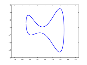
(a)

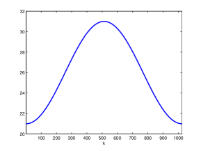
(b)

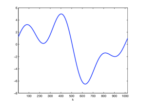
(c)

Figure 3: LABEL:sub@fig.meanpattern0 Plot of the mean pattern $\boldsymbol{f}\vphantom{f}=(\boldsymbol{f}\vphantom{f}^{(1)},\boldsymbol{f}\vphantom{f}^{(2)})$ used in the simulations with $k=1024$. LABEL:sub@fig.meanpattern1 The first coordinates $\boldsymbol{f}\vphantom{f}^{(1)}$. LABEL:sub@fig.meanpattern2 The second coordinates $\boldsymbol{f}\vphantom{f}^{(2)}$.

White noise :

the random variable $\tilde{}\boldsymbol{\zeta}=(\zeta_{1}^{(1)},\zeta_{2}^{(1)},\ldots,\zeta_{1}^{(k)},\zeta_{2}^{(k)})^{\prime}\in\mathbb{R}^{2k}$ is a centered Gaussian vector of variance

$$\boldsymbol{\Sigma}_{1}=4Id_{2k}.$$

We have $\gamma_{\max}(k)=4$ and this correspond to an isotropic Gaussian noise as in [Kent & Mardia, 1997, Le, 1998], see Figure 6.

Weakly correlated noise :

the random variable $\tilde{}\boldsymbol{\zeta}$ is a centered Gaussian vector of variance $\boldsymbol{\Sigma}_{2}$ with

$$\boldsymbol{\Sigma}^{\frac{1}{2}}_{2}=Id_{2}\otimes\left[\tfrac{1}{2}\exp\left(-\tfrac{\lvert\ell-\ell^{\prime}\rvert}{100}^{2}\right)\right]_{\ell,\ell^{\prime}=1}^{k}$$

Hence, $\boldsymbol{\Sigma}_{2}$ is a Toeplitz matrix and it follows from classical matrix theory, see e.g. [Horn & Johnson, 1990], that $\gamma_{\max}(k)$ is bounded (here $\gamma_{\max}\leq 80$). See Figure 6.

Highly correlated noise :

the random variable $\tilde{}\boldsymbol{\zeta}$ is a centered Gaussian vector of variance

$$\boldsymbol{\Sigma}_{3}=Id_{2}\otimes P\operatorname*{\mbox{Diag}}\left(\tfrac{\ell^{2}}{2k},\ \ell=1,\ldots,k\right)P^{\prime}$$

where $P$ is an arbitrary matrix in $\mathbf{SO}(k)$. Hence, in this case $\gamma_{\max}(k)=\frac{k}{4}$ and the level of noise increase with $k$, see Figure 6.

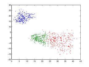
(a) Observations $\mathbf{Y}$

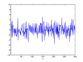
(b) A realization of $\boldsymbol{\zeta}_{1}$

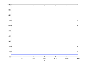
(c) Spectrum of $\boldsymbol{\Sigma}_{1}$

Figure 4: Example of data generated by model (1.1) with white noise.

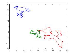
(a) Observations $\mathbf{Y}$

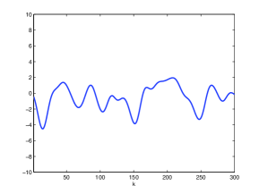
(b) A realization of $\boldsymbol{\zeta}_{1}$

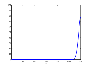
(c) Spectrum of $\boldsymbol{\Sigma}_{2}$

Figure 5: Example of data generated by model (1.1) with weakly correlated noise.

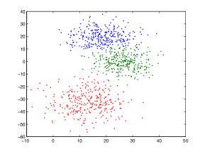
(a) Observations $\mathbf{Y}$

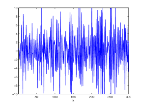
(b) A realization of $\boldsymbol{\zeta}_{1}$

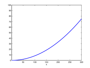
(c) Spectrum of $\boldsymbol{\Sigma}_{3}$

Figure 6: Example of observations generated by model (1.1) with the highly correlated noise.

6.2 Description of the procedure

The estimation procedure follows the guidelines described in Section 4. We are testing the effect of the number $J$ of observations and the number $k$ of landmarks on the estimation of the parameters of interest of model (1.1). All the simulations are performed with $J=10,100,500$ and $k=20,50,100,1000,3000$ and for each combination of these two factors the simulations are performed with $M=30$ repetitions of model (1.1).

Moreover, estimations are done without and with the pre-smoothing step. In the former case we have $\lambda(k)=\frac{k}{2}$, that is, there is no reduction of the dimension. In the latter case, the smoothing parameter $\lambda(k)$ is fixed manually to ensure a proper reconstruction of the mean pattern $f$. Note that we need $\lambda>7$ to get correct results and we took $\lambda_{20}=\lambda_{50}=\lambda_{100}=7$, $\lambda_{1000}=11$ and $\lambda_{3000}=25$.

We use a quasi-Newton trust-region based algorithm to solve the optimization problems (4.3) and (4.4). The formula for the gradient is given in (B.1). All the computations are performed with Matlab.

6.3 Results: estimation of the mean pattern

For each of the $30$ repetitions of model (1.1) with the possible values of $k$ and $J$, we compute the quantities $\frac{1}{k}\|\hat{\boldsymbol{f}}\vphantom{f}\vphantom{\boldsymbol{f}\vphantom{f}}^{\lambda}-\boldsymbol{f}\vphantom{f}^{*}_{\boldsymbol{\Theta}_{0}}\|^{2}_{\mathbb{R}^{k\times 2}}$ where $\hat{\boldsymbol{f}}\vphantom{f}\vphantom{\boldsymbol{f}\vphantom{f}}^{\lambda}$ corresponds to the smoothed Procrustes mean of the observations defined in (1.8) and, $\frac{1}{k}\|\hat{\boldsymbol{f}}\vphantom{f}-\boldsymbol{f}\vphantom{f}^{*}_{\boldsymbol{\Theta}_{0}}\|^{2}_{\mathbb{R}^{k\times 2}}$ where $\hat{\boldsymbol{f}}\vphantom{f}$ is the (non smoothed) Procrustes mean of the data. Recall that $\boldsymbol{f}\vphantom{f}_{\boldsymbol{\Theta}_{0}}$ is defined by formula (5.3).

Boxplots of the results are given in Figures 9, 9 and 9 for the different kinds of error terms described in Section 6.1. In the figures, the abscissa represents the different values of the number $k$ of landmarks and boxplots in red correspond to $J=10$ observations, in green to $J=100$ observations and in blue to $J=500$ observations.

The estimation of the mean pattern with the white noise error term is given by Figure 9. In Figure 7a, for a fixed $k$, the non-smoothed version $\frac{1}{k}\|\hat{\boldsymbol{f}}\vphantom{f}-\boldsymbol{f}\vphantom{f}^{*}\|^{2}_{\mathbb{R}^{k\times 2}}$ decreases when $J$ increases. Moreover, the values of $\frac{1}{k}\|\hat{\boldsymbol{f}}\vphantom{f}-\boldsymbol{f}\vphantom{f}^{*}\|^{2}_{\mathbb{R}^{k\times 2}}$ remain stable when $J$ remains fixed and $k$ increases. Recall that this framework corresponds to the isotropic Gaussian noise described in [Kent & Mardia, 1997]. The simulations seem to confirm their conclusions and show that in this framework the dimension $k$ is not preponderant. In Figure 7b, the smoothed version $\frac{1}{k}\|\hat{\boldsymbol{f}}\vphantom{f}\vphantom{\boldsymbol{f}\vphantom{f}}^{\lambda}-\boldsymbol{f}\vphantom{f}\|^{2}_{\mathbb{R}^{k\times 2}}$ decreases when $J$ and $k$ increase. The main difference with the non-smoothed estimation is the convergence to 0 of $\frac{1}{k}\|\hat{\boldsymbol{f}}\vphantom{f}\vphantom{\boldsymbol{f}\vphantom{f}}^{\lambda}-\boldsymbol{f}\vphantom{f}\|^{2}_{\mathbb{R}^{k\times 2}}$ when $J$ remains fixed and $k$ increases.

In Figure 9, the results of the estimation of the mean pattern are plotted for the weakly correlated noise term. Figure 7a shows us a similar behavior of the non-smoothed Procrustes mean but with non-decreasing values of $\frac{1}{k}\|\hat{\boldsymbol{f}}\vphantom{f}\vphantom{\boldsymbol{f}\vphantom{f}}^{\lambda}-\boldsymbol{f}\vphantom{f}^{*}\|^{2}_{\mathbb{R}^{k\times 2}}$ when $k$ increases and $J$ remains fixed. In Figure 7b, the smoothed Procrustes mean converges as $k$ goes to infinity and the bigger $J$ is the faster the convergence is.

The results of the estimations of the mean pattern with the highly correlated noise are presented Figure 9. The results that appear in Figure 8a are quite different compared to those presented Figures 7a and 7a. The estimation seems to be worst when $k$ increases and $J$ remains fixed. The reason is that the level of noise, measured by $\gamma_{\max}(k)$ is increasing with $k$. The smoothing step is efficient and the estimations presented Figure 8b have a similar behavior to those given in Figures 7b and 7b.

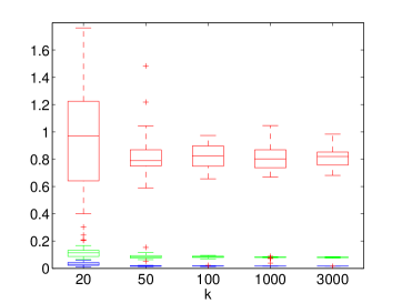
(a) f

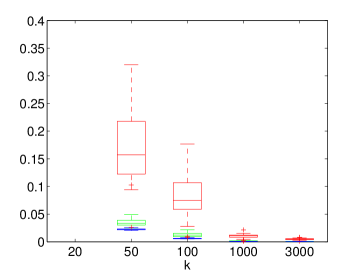
(b) f

Figure 7: Estimation of the mean pattern with the white noise. Boxplot in red correspond to $J=10$, in green to $J=100$ and in blue to $J=500$.

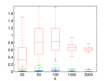
(a) f

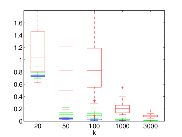
(b) f

Figure 8: Estimation of the mean pattern with the weakly correlated noise. Boxplot in red correspond to $J=10$, in green to $J=100$ and in blue to $J=500$.

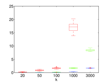
(a) f

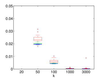
(b) f

Figure 9: Estimation of the mean pattern with the highly correlated noise. Boxplot in red correspond to $J=10$, in green to $J=100$ and in blue to $J=500$.

Appendix A Proofs

A.1 Proof of Lemma 4.1

Using the decomposition (4.2), we obtain the following identity

$$M^{\lambda}(\boldsymbol{a},\boldsymbol{\alpha},\boldsymbol{b}\vphantom{b})=M^{\lambda}_{0}(\boldsymbol{a},\boldsymbol{\alpha})+\bar{M}(\boldsymbol{a},\boldsymbol{\alpha},\boldsymbol{b}\vphantom{b}).$$ (A.1)

Note that we have used the fact that the subspaces $\mathcal{V}^{\lambda}_{0}$ and $\bar{\mathcal{V}}$ are orthogonal and that $\bar{A}\mathds{1}_{k}\otimes b_{j}=\mathds{1}_{k}\otimes b_{j}$, for all $b_{j}\in\mathbb{R}^{2}$. Let us also introduce the notation $\bar{\mathbf{Y}}_{j}=\frac{1}{k}\sum_{\ell=1}^{k}[\mathbf{Y}_{j}]_{\ell}\in\mathbb{R}^{2}$, that is $\bar{A}\mathbf{Y}_{j}=\mathds{1}_{k}\otimes\bar{\mathbf{Y}}_{j}\in\mathbb{R}^{k\times 2}$ is a degenerated configuration, and $\bar{\mathbf{Y}}=\frac{1}{J}\sum_{j=1}^{J}\bar{\mathbf{Y}}_{j}\in\mathbb{R}^{2}$. For a fixed $(\boldsymbol{a},\boldsymbol{\alpha})\in\mathbb{R}^{J}\times[-\pi,\pi[^{J}$, the functional $\boldsymbol{b}\vphantom{b}\longmapsto\bar{M}(\boldsymbol{a},\boldsymbol{\alpha},\boldsymbol{b}\vphantom{b})$ vanishes if and only if there exists a $b_{0}\in\mathbb{R}^{2}$ such that $e^{-a_{j}}(\bar{A}\mathbf{Y}_{j}-\mathds{1}_{k}\otimes b_{j})R_{-\alpha_{j}}=\mathds{1}_{k}\otimes b_{0}$ for all $j=1,\ldots,J$. Therefore, for this fixed $(\boldsymbol{a},\boldsymbol{\alpha})$, there is a unique point $\boldsymbol{b}\vphantom{b}=\boldsymbol{b}\vphantom{b}(\boldsymbol{a},\boldsymbol{\alpha}):=(\bar{\mathbf{Y}}_{1}-e^{a_{1}}\bar{\mathbf{Y}}(\overline{e^{\boldsymbol{a}}R_{\boldsymbol{\alpha}}})^{-1}R_{\alpha_{1}},\ldots,\bar{\mathbf{Y}}_{J}-e^{a_{J}}\bar{\mathbf{Y}}(\overline{e^{\boldsymbol{a}}R_{\boldsymbol{\alpha}}})^{-1}R_{\alpha_{J}})$ with $\overline{e^{\boldsymbol{a}}R_{\boldsymbol{\alpha}}}=\frac{1}{J}\sum_{j=1}^{J}e^{a_{j}}R_{\alpha_{j}}\in\mathbb{R}^{2\times 2}$ and which satisfies,

$$\boldsymbol{b}\vphantom{b}(\boldsymbol{a},\boldsymbol{\alpha})=\operatorname*{\mbox{argmin}}_{\boldsymbol{b}\vphantom{b}\in\boldsymbol{\Theta}^{\boldsymbol{b}\vphantom{b}}_{0}}\bar{M}(\boldsymbol{a},\boldsymbol{\alpha},\boldsymbol{b}\vphantom{b})$$

Thence, thanks to the decomposition (A.1) and the fact that $\bar{M}(\boldsymbol{a},\boldsymbol{\alpha},\boldsymbol{b}\vphantom{b}(\boldsymbol{a},\boldsymbol{\alpha}))=0$, we have

$$\operatorname*{\mbox{argmin}}_{(\boldsymbol{a},\boldsymbol{\alpha},\boldsymbol{b}\vphantom{b})\in\boldsymbol{\Theta}_{0}}M^{\lambda}(\boldsymbol{a},\boldsymbol{\alpha},\boldsymbol{b}\vphantom{b})=\bigg{(}\operatorname*{\mbox{argmin}}_{(\boldsymbol{a},\boldsymbol{\alpha})\in\boldsymbol{\Theta}^{\boldsymbol{a},\boldsymbol{\alpha}}_{0}}M^{\lambda}_{0}(\boldsymbol{a},\boldsymbol{\alpha})\ ,\ \boldsymbol{b}\vphantom{b}\Big{(}\operatorname*{\mbox{argmin}}_{(\boldsymbol{a},\boldsymbol{\alpha})\in\boldsymbol{\Theta}^{\boldsymbol{a},\boldsymbol{\alpha}}_{0}}M^{\lambda}_{0}(\boldsymbol{a},\boldsymbol{\alpha})\Big{)}\bigg{)},$$

and the claim is proved. ∎

A.2 Proof of Theorem 5.1

For all $(\hat{}\boldsymbol{a}^{\lambda},\hat{}\boldsymbol{\alpha}^{\lambda})\in\boldsymbol{\Theta}^{\boldsymbol{a},\boldsymbol{\alpha}}_{0}$ and $(\boldsymbol{a}^{*},\boldsymbol{\alpha}^{*})\in[-A,A]\times[-\mathcal{A},\mathcal{A}]$, we have the following inequality

$$\frac{1}{J}\lVert(\hat{}\boldsymbol{a}^{\lambda},\hat{}\boldsymbol{\alpha}^{\lambda})-(\boldsymbol{a}^{*},\boldsymbol{\alpha}^{*})\rVert^{2}_{\mathbb{R}^{2J}}\leq\frac{2}{J}\lVert(\hat{}\boldsymbol{a}^{\lambda},\hat{}\boldsymbol{\alpha}^{\lambda})-(\boldsymbol{a}^{*}_{\boldsymbol{\Theta}_{0}},\boldsymbol{\alpha}^{*}_{\boldsymbol{\Theta}_{0}})\rVert^{2}_{\mathbb{R}^{2J}}+\frac{2}{J}\lVert(\boldsymbol{a}^{*}_{\boldsymbol{\Theta}_{0}},\boldsymbol{\alpha}^{*}_{\boldsymbol{\Theta}_{0}})-(\boldsymbol{a}^{*},\boldsymbol{\alpha}^{*})\rVert^{2}_{\mathbb{R}^{2J}}.$$

The proof of Theorem 5.1 is a direct consequence of Proposition A.1 and Lemma A.2 below which control the convergence in probability of the two terms in the right hand side in the preceding inequality.

Proposition A.1.

Consider model (1.1) and suppose that Assumptions 1 and 2 hold and that Assumption 3 is verified with $A,\mathcal{A}<0.1$. If $\lambda=\lambda(k)=k^{\frac{1}{2s+1}}$ then there exists a constant $C(L,s,A,\mathcal{A},\boldsymbol{f}\vphantom{f}_{0})$ such that for all $x>0$

$$\mathbb{P}\left(\frac{1}{J}\lVert(\hat{}\boldsymbol{a}^{\lambda},\hat{}\boldsymbol{\alpha}^{\lambda})-(\boldsymbol{a}^{*}_{\boldsymbol{\Theta}_{0}},\boldsymbol{\alpha}^{*}_{\boldsymbol{\Theta}_{0}})\rVert^{2}_{\mathbb{R}^{2J}}\geq C(L,s,A,\mathcal{A},\boldsymbol{f}\vphantom{f}_{0})\left(F\big{(}k^{-\frac{2s}{2s+1}}\big{)}+F\big{(}V_{1}(k,J,x)\big{)}\right)\right)\leq 2e^{-x},$$

where $V_{1}(k,J,x)=3\gamma_{\max}(k)k^{-\frac{2s}{2s+1}}\left(1+\sqrt{2\frac{x}{Jk}}+2\frac{x}{Jk}\right)$ and $F:\mathbb{R}^{+}\longrightarrow\mathbb{R}$, with $F(u)=u+\sqrt{u}$.

The proof of Proposition A.1 is postponed to Section A.5. The following lemma is a direct consequence of Bernstein’s inequality for bounded random variables, see e.g. Proposition 2.9 in [Massart, 2007].

Lemma A.2.

Suppose that Assumption 3 holds and that the random variables $(a^{*}_{j},\alpha^{*}_{j})$, $j=1,\ldots,J$ have zero expectation in $[-A,A]\times[-\mathcal{A},\mathcal{A}]$. Then, for any $x>0$, we have

$$\mathbb{P}\left(\frac{1}{J}\lVert(\boldsymbol{a}^{*}_{\boldsymbol{\Theta}_{0}},\boldsymbol{\alpha}^{*}_{\boldsymbol{\Theta}_{0}})-(\boldsymbol{a}^{*},\boldsymbol{\alpha}^{*})\rVert^{2}_{\mathbb{R}^{2J}}\geq C(A,\mathcal{A})\Big{(}\sqrt{\tfrac{2x}{J}}+\tfrac{x}{3J}\Big{)}^{2}\right)\leq 4e^{-x},$$

where $C(A,\mathcal{A})=4\max\{A^{2},\mathcal{A}^{2}\}$.∎

A.3 Proof of Theorem 5.2

The proof of Theorem 5.2 follows the same guideline as the proof of Theorem 5.1. Consider the inequality

$$\frac{1}{J}\lVert\hat{}\boldsymbol{b}\vphantom{b}\vphantom{\boldsymbol{b}\vphantom{b}}^{\lambda}-\boldsymbol{b}\vphantom{b}^{*}\rVert^{2}_{\mathbb{R}^{2J}}\leq\frac{2}{J}\lVert\hat{}\boldsymbol{b}\vphantom{b}\vphantom{\boldsymbol{b}\vphantom{b}}^{\lambda}-\boldsymbol{b}\vphantom{b}^{*}_{\boldsymbol{\Theta}_{0}}\rVert^{2}_{\mathbb{R}^{2J}}+\frac{2}{J}\lVert\boldsymbol{b}\vphantom{b}^{*}_{\boldsymbol{\Theta}_{0}}-\boldsymbol{b}\vphantom{b}^{*}\rVert^{2}_{\mathbb{R}^{2J}}.$$

Theorem 5.2 is now a direct consequence of Proposition A.3 and Lemma A.4.

Proposition A.3.

Under the hypothesis of Proposition A.1, there exists a constant $C(L,s,A,\mathcal{A},\linebreak[1]B,\boldsymbol{f}\vphantom{f})>0$ such that for all $x>0$,

$$\mathbb{P}\left(\frac{2}{J}\lVert\hat{}\boldsymbol{b}\vphantom{b}\vphantom{\boldsymbol{b}\vphantom{b}}^{\lambda}-\boldsymbol{b}\vphantom{b}_{\boldsymbol{\Theta}_{0}}^{*}\rVert^{2}_{\mathbb{R}^{2J}}\geq C(L,s,A,\mathcal{A},B,\boldsymbol{f}\vphantom{f})\Big{(}F(k^{-\frac{-2s}{2s+1}})+F(V_{1}(k,J,x))+V_{2}(k,J,x)\Big{)}\right)\leq 5e^{-x},$$

where $V_{1}(k,J,x)=3\gamma_{\max}(k)k^{-\frac{2s}{2s+1}}\left(1+\sqrt{2\frac{x}{Jk}}+2\frac{x}{Jk}\right)$, $V_{2}(k,J,x)=\frac{4}{k}\gamma_{\max}(k)\big{(}1+\sqrt{2\frac{x}{J}}+\frac{x}{J}\big{)}$ and $F(u)=u+\sqrt{u}$, $u\geq 0$.

The proof of Proposition A.3 is postponed to Section A.6.

Lemma A.4.

Suppose that Assumption 3 holds with $\mathcal{A}<\frac{\pi}{4}$ and that the random variables $(a^{*}_{j},\alpha^{*}_{j},b^{*}_{j})$ $j=1,\ldots,J$ have zero expectation in $\Theta\subset\mathbb{R}^{4J}$. For any $x>0$ , we have

$$\mathbb{P}\Big{(}\frac{2}{J}\lVert\boldsymbol{b}\vphantom{b}^{*}_{\boldsymbol{\Theta}_{0}}-\boldsymbol{b}\vphantom{b}^{*}\rVert^{2}_{\mathbb{R}^{2J}}\geq C(A,\mathcal{A},B)\Big{(}\sqrt{\tfrac{2x}{J}}+\tfrac{x}{3J}\Big{)}^{2}\Big{)}\leq 4e^{-x},$$

where $C(A,\mathcal{A},B)=8B^{2}e^{4A}(\cos\mathcal{A}-\sin\mathcal{A})^{-2}$.

Proof.

This result is a consequence of the Bernstein’s inequality for bounded random variable. We have

$$\lVert\boldsymbol{b}\vphantom{b}^{*}_{\boldsymbol{\Theta}_{0}}-\boldsymbol{b}\vphantom{b}^{*}\rVert_{\mathbb{R}^{2J}}=\sqrt{\sum_{j=1}^{J}\lVert e^{a_{j}^{*}}\bar{}\boldsymbol{b}\vphantom{b}^{*}(\overline{e^{\boldsymbol{a}}R_{\boldsymbol{\alpha}}})^{-1}R_{\alpha^{*}_{j}}\rVert^{2}_{\mathbb{R}^{2}}}\leq e^{A}\sqrt{J}\lVert\bar{}\boldsymbol{b}\vphantom{b}^{*}(\overline{e^{\boldsymbol{a}^{*}}R_{\boldsymbol{\alpha}^{*}}})^{-1}\rVert_{\mathbb{R}^{2}},$$

where $\overline{e^{\boldsymbol{a}^{*}}R_{\boldsymbol{\alpha}^{*}}}=\frac{1}{J}\sum_{j=1}^{J}e^{a^{*}_{j}}R_{\alpha_{j}^{*}}$ is an invertible $2\times 2$ matrix whose smallest eigenvalue is greater than $e^{-A}(\cos\mathcal{A}-\sin\mathcal{A})>0$ as $\mathcal{A}<\frac{\pi}{4}$. To see this, remark that the eigenvalues of $\overline{e^{\boldsymbol{a}^{*}}R_{\boldsymbol{\alpha}^{*}}}$ are $\frac{1}{J}\sum_{j=1}^{J}e^{a^{*}_{j}}(\cos\alpha^{*}_{j}\pm i\sin\alpha^{*}_{j})$ and we have $\big{|}\frac{1}{J}\sum_{j=1}^{J}e^{a^{*}_{j}}(\cos\alpha^{*}_{j}\pm i\sin\alpha^{*}_{j})\big{|}\geq e^{-A}(\cos\mathcal{A}-\sin\mathcal{A})>0$. We now have

$$\frac{1}{\sqrt{J}}\lVert\boldsymbol{b}\vphantom{b}^{*}_{\boldsymbol{\Theta}_{0}}-\boldsymbol{b}\vphantom{b}^{*}\rVert_{\mathbb{R}^{2J}}\leq C(A,\mathcal{A})\lVert\bar{}\boldsymbol{b}\vphantom{b}^{*}\rVert_{\mathbb{R}^{2}},$$

where $C(A,\mathcal{A})=e^{2A}(\cos\mathcal{A}-\sin\mathcal{A})^{-1}$. Finally, for all $u>0$ we have $\mathbb{P}(\frac{1}{\sqrt{J}}\lVert\boldsymbol{b}\vphantom{b}^{*}_{\boldsymbol{\Theta}_{0}}-\boldsymbol{b}\vphantom{b}^{*}\rVert_{\mathbb{R}^{2J}}\geq u)\leq\mathbb{P}(C(A,\mathcal{A})\lVert\bar{}\boldsymbol{b}\vphantom{b}^{*}\rVert_{\mathbb{R}^{2}}\geq u)$ and a Bernstein type inequality (see e.g. Proposition 2.9 in [Massart, 2007]) gives us $\mathbb{P}\Big{(}\lVert\bar{}\boldsymbol{b}\vphantom{b}^{*}\rVert_{\mathbb{R}^{2}}\geq 2B\big{(}\sqrt{\tfrac{2x}{J}}+\tfrac{x}{3J}\big{)}\Big{)}\leq 4e^{-x}$ which yields

$$\mathbb{P}\Big{(}\frac{1}{J}\lVert\boldsymbol{b}\vphantom{b}^{*}_{\boldsymbol{\Theta}_{0}}-\boldsymbol{b}\vphantom{b}^{*}\rVert^{2}_{\mathbb{R}^{2J}}\geq C(A,\mathcal{A},B)\Big{(}\sqrt{\tfrac{2x}{J}}+\tfrac{x}{3J}\Big{)}^{2}\Big{)}\leq 4e^{-x},$$

where $C(A,\mathcal{A},B)=4B^{2}e^{4A}(\cos\mathcal{A}-\sin\mathcal{A})^{-2}$. ∎

A.4 Proof of Theorem 5.3

Recall the notations introduced Section 2.1: for $\hat{g}^{\lambda}_{j}=(\hat{a}^{\lambda}_{j},\hat{\alpha}_{j}^{\lambda},\hat{b}_{j}^{\lambda})$ we have $\hat{g}^{\lambda}_{j}.\boldsymbol{f}\vphantom{f}=e^{\hat{a}^{\lambda}_{j}}\boldsymbol{f}\vphantom{f}R_{\hat{\alpha}_{j}^{\lambda}}+\hat{b}_{j}^{\lambda}$. Then, we have

$$\frac{1}{k}\Big{\|}\hat{\boldsymbol{f}}\vphantom{f}\vphantom{\boldsymbol{f}\vphantom{f}}^{\lambda}-\boldsymbol{f}\vphantom{f}\Big{\|}^{2}_{\mathbb{R}^{k\times 2}} =\frac{1}{k}\Big{\|}\frac{1}{J}\sum_{j=1}^{J}(\hat{g}^{\lambda}_{j})^{-1}.(\mathbf{A}^{\lambda}\mathbf{Y}_{j})-\boldsymbol{f}\vphantom{f}\Big{\|}^{2}_{\mathbb{R}^{k\times 2}}$$

$$\leq\frac{2}{kJ}\sum_{j=1}^{J}\Big{\|}\mathbf{A}^{\lambda}\Big{(}(\hat{g}^{\lambda}_{j})^{-1}.\mathbf{Y}_{j}-\boldsymbol{f}\vphantom{f}\Big{)}\Big{\|}^{2}_{\mathbb{R}^{k\times 2}}+\frac{2}{k}\Big{\|}\mathbf{A}^{\lambda}\boldsymbol{f}\vphantom{f}-\boldsymbol{f}\vphantom{f}\Big{\|}^{2}_{\mathbb{R}^{k\times 2}}$$

$$\leq\underbrace{\frac{4}{kJ}\sum_{j=1}^{J}\Big{\|}\mathbf{A}^{\lambda}\Big{(}(g^{\lambda}_{j})^{-1}.g^{*}_{j}.\boldsymbol{f}\vphantom{f}-\boldsymbol{f}\vphantom{f}\Big{)}\Big{\|}^{2}_{\mathbb{R}^{k\times 2}}+\Big{\|}e^{a_{j}^{*}-\hat{a}_{j}^{\lambda}}\mathbf{A}^{\lambda}\boldsymbol{\zeta}_{j}R_{\alpha_{j}^{*}-\hat{\alpha}_{j}^{\lambda}}\Big{\|}^{2}_{\mathbb{R}^{k\times 2}}}_{\mathbf{V}}+\underbrace{\vphantom{\frac{4}{kJ}\sum_{j=1}^{J}}\frac{2}{k}\Big{\|}\mathbf{A}^{\lambda}\boldsymbol{f}\vphantom{f}-\boldsymbol{f}\vphantom{f}\Big{\|}^{2}_{\mathbb{R}^{k\times 2}}}_{\mathbf{B}}.$$

The rest of the proof is devoted to control the terms $\mathbf{B}$ and $\mathbf{V}$. The term $\mathbf{B}$ is controlled by the bias of the low pass filter. According to Lemma B.1, if Assumption 1 holds and by choosing the optimal frequency cutoff $\lambda=\lambda(k)=k^{\frac{1}{2s+1}}$, there exists a constant $C(L,s)>0$ such that

$$\mathbf{B}=\frac{2}{k}\|\mathbf{A}^{\lambda}\boldsymbol{f}\vphantom{f}-\boldsymbol{f}\vphantom{f}\|^{2}_{\mathbb{R}^{k\times 2}}\leq C(L,s)k^{-\frac{2s}{2s+1}}.$$ (A.2)

The term $\mathbf{V}$ contains two expressions. To bound the first one we use Bessel’s inequality and Lemma B.4. More precisely, we have for all $j=1,\ldots,J$

$$\frac{1}{k}\big{\|}\mathbf{A}^{\lambda}\big{(}(g^{\lambda}_{j})^{-1}.g^{*}_{j}.\boldsymbol{f}\vphantom{f}-\boldsymbol{f}\vphantom{f}\big{)}\big{\|}^{2}_{\mathbb{R}^{k\times 2}} \leq\frac{1}{k}\big{\|}(g^{\lambda}_{j})^{-1}.g^{*}_{j}.\boldsymbol{f}\vphantom{f}-\boldsymbol{f}\vphantom{f}\big{\|}^{2}_{\mathbb{R}^{k\times 2}}$$

$$\leq C(A,\boldsymbol{f}\vphantom{f})\big{\|}(a^{*}_{j}-\hat{a}^{\lambda}_{j},\alpha^{*}_{j}-\hat{\alpha}^{\lambda}_{j},e^{\hat{a}^{\lambda}_{j}}(b^{*}_{j}-\hat{b}\vphantom{b}^{\lambda}_{j})R_{-\hat{\alpha}_{j}^{\lambda}})\big{\|}^{2}_{\mathbb{R}^{4}}$$

$$\leq C(A,\boldsymbol{f}\vphantom{f})\big{\|}(a^{*}_{j}-\hat{a}^{\lambda}_{j},\alpha^{*}_{j}-\hat{\alpha}^{\lambda}_{j})\big{\|}^{2}_{\mathbb{R}^{2}}+C(A,\boldsymbol{f}\vphantom{f})\big{\|}b^{*}_{j}-\hat{b}\vphantom{\boldsymbol{b}\vphantom{b}}^{\lambda}_{j}\big{\|}^{2}_{\mathbb{R}^{2}}$$

We can now use Theorem 5.1 and 5.2 to derive the following concentration inequality,

$$\begin{split}\mathbb{P}\bigg{(}\frac{4}{kJ}\sum_{j=1}^{J}\big{\|}\mathbf{A}^{\lambda}\big{(}(&g^{\lambda}_{j})^{-1}.g^{*}_{j}.\boldsymbol{f}\vphantom{f}-\boldsymbol{f}\vphantom{f}\big{)}\big{\|}^{2}_{\mathbb{R}^{k\times 2}}\\ &\geq C(L,s,A,\mathcal{A},B,\boldsymbol{f}\vphantom{f})\Big{(}A_{1}(k,J,x)+A_{3}(k,J,x)+A_{2}(J,x)\Big{)}\bigg{)}\leq 13e^{-x}\end{split}$$ (A.3)

where $C(L,s,A,\mathcal{A},B,\boldsymbol{f}\vphantom{f})>0$ is a constant independent of $k$ and $J$ and $A_{1},A_{2},A_{3}$ are defined in the statement of Theorem 5.1 and 5.2. The second term contained in $\mathbf{V}$ is treated by equation (A.10) below. Hence, formulas (A.3) and (A.10) yield

$$\mathbb{P}\bigg{(}\mathbf{V}\geq C(L,s,A,\mathcal{A},B,\boldsymbol{f}\vphantom{f})\Big{(}A_{1}(k,J,x)+A_{3}(k,J,x)+A_{2}(J,x)\Big{)}\bigg{)}\leq 14e^{-x},$$ (A.4)

for some constant $C(L,s,A,\mathcal{A},B,\boldsymbol{f}\vphantom{f})>0$. Putting together equations (A.2) and (A.4) gives

$$\mathbb{P}\bigg{(}\frac{1}{k}\lVert\hat{\boldsymbol{f}}\vphantom{f}\vphantom{\boldsymbol{f}\vphantom{f}}^{\lambda}-\boldsymbol{f}\vphantom{f}\rVert^{2}_{\mathbb{R}^{k\times 2}}\geq C(L,s,A,\mathcal{A},B,\boldsymbol{f}\vphantom{f})\Big{(}A_{1}(k,J,x)+A_{3}(k,J,x)+A_{2}(J,x)\Big{)}\bigg{)}\leq 14e^{-x}.$$

for some constant $C(L,s,A,\mathcal{A},B,\boldsymbol{f}\vphantom{f})>0$. The proof of Theorem 5.3 is completed. ∎

A.5 Proof of Proposition A.1

The mean pattern $\boldsymbol{f}\vphantom{f}$ can be decomposed as $\boldsymbol{f}\vphantom{f}=\bar{\boldsymbol{f}}\vphantom{f}+\boldsymbol{f}\vphantom{f}_{0}\in\boldsymbol{1}_{k\times 2}^{\vphantom{\perp}}\oplus\boldsymbol{1}_{k\times 2}^{\perp}$. Then, $\boldsymbol{f}\vphantom{f}_{0}$ is the centered version of $\boldsymbol{f}\vphantom{f}$ and we can consider the criterion,

$$D_{0}(\boldsymbol{a},\boldsymbol{\alpha})=\frac{1}{Jk}\sum_{j=1}^{J}\bigg{\lVert}e^{a^{*}_{j}-a_{j}}\boldsymbol{f}\vphantom{f}_{0}R_{\alpha^{*}_{j}-\alpha_{j}}-\frac{1}{J}\sum_{j^{\prime}=1}^{J}e^{a^{*}_{j^{\prime}}-a_{j^{\prime}}}\boldsymbol{f}\vphantom{f}_{0}R_{\alpha^{*}_{j^{\prime}}-\alpha_{j^{\prime}}}\bigg{\rVert}^{2}_{\mathbb{R}^{k\times 2}}.$$

We now have,

$$(\hat{}\boldsymbol{a}^{\lambda},\hat{}\boldsymbol{\alpha}^{\lambda})=\operatorname*{\mbox{argmin}}_{(\boldsymbol{a},\boldsymbol{\alpha})\in\boldsymbol{\Theta}_{0}^{\boldsymbol{a},\boldsymbol{\alpha}}}M_{0}^{\lambda}(\boldsymbol{a},\boldsymbol{\alpha})\qquad\text{ and }\qquad(\boldsymbol{a}^{*}_{\boldsymbol{\Theta}_{0}},\boldsymbol{\alpha}^{*}_{\boldsymbol{\Theta}_{0}})=\operatorname*{\mbox{argmin}}_{(\boldsymbol{a},\boldsymbol{\alpha})\in\boldsymbol{\Theta}_{0}^{\boldsymbol{a},\boldsymbol{\alpha}}}D_{0}(\boldsymbol{a},\boldsymbol{\alpha}).$$

Then, the convergence of $(\hat{}\boldsymbol{a}^{\lambda},\hat{}\boldsymbol{\alpha}^{\lambda})$ to $(\boldsymbol{a}^{*}_{\boldsymbol{\Theta}_{0}},\boldsymbol{\alpha}^{*}_{\boldsymbol{\Theta}_{0}})$ is guaranteed if $(\boldsymbol{a}^{*}_{\boldsymbol{\Theta}_{0}},\boldsymbol{\alpha}^{*}_{\boldsymbol{\Theta}_{0}})$ is uniquely defined and if there is a uniform convergence in probability of $M_{0}^{\lambda}$ to $D_{0}$, see e.g. [van der Vaart, 1998]. This is the aim of Lemmas A.5 and A.6 below.

Lemma A.5.

Let $\boldsymbol{f}\vphantom{f}$ be a non-degenerated configuration in $\mathbb{R}^{k\times 2}$, i.e. $\boldsymbol{f}\vphantom{f}\notin\boldsymbol{1}_{k\times 2}$. Then, the argmin of $D_{0}$ on $\boldsymbol{\Theta}_{0}^{\boldsymbol{a},\boldsymbol{\alpha}}$ is unique and denoted by $(\boldsymbol{a}_{\boldsymbol{\Theta}_{0}}^{*},\boldsymbol{\alpha}_{\boldsymbol{\Theta}_{0}}^{*})=(a_{j}-\bar{}\boldsymbol{a}^{*},\alpha_{j}-\bar{}\boldsymbol{\alpha}^{*})$, where $\bar{\boldsymbol{a}}^{*}=\frac{1}{J}\sum_{j=1}^{J}a_{j}^{*}$, $\bar{}\boldsymbol{\alpha}^{*}=\frac{1}{J}\sum_{j=1}^{J}\alpha_{j}^{*}$.

Proof.

As $\boldsymbol{f}\vphantom{f}$ is a non-degenerated configuration, we have $\boldsymbol{f}\vphantom{f}_{0}\neq 0$. Thus, the stabilizer of $\boldsymbol{f}\vphantom{f}$ is reduced to the identity, see Section 2.1. Then $D_{0}(\boldsymbol{a},\boldsymbol{\alpha})=0$ if and only if there exists $(a_{0},\alpha_{0})\in\mathbb{R}^{2}$ such that $(\boldsymbol{a},\boldsymbol{\alpha})=(\boldsymbol{a}^{*},\boldsymbol{\alpha}^{*})*(a_{0},\alpha_{0})=(a_{1}^{*}+a_{0},\alpha^{*}_{1}+\alpha_{0},\ldots,a_{J}+a_{0},\alpha_{J}^{*}+\alpha_{0})$. By choosing $(a_{0},\alpha_{0})=(-\bar{\boldsymbol{a}}^{*},-\bar{}\boldsymbol{\alpha}^{*})$ we have $\sum_{j=1}^{J}(a^{*}_{j},\alpha^{*}_{j})*(a_{0},\alpha_{0})=0$. That is $(\boldsymbol{a}^{*}_{\boldsymbol{\Theta}_{0}},\boldsymbol{\alpha}^{*}_{\boldsymbol{\Theta}_{0}})=(\boldsymbol{a}^{*},\boldsymbol{\alpha}^{*})*(a_{0},\alpha_{0})\in\boldsymbol{\Theta}_{0}^{\boldsymbol{a},\boldsymbol{\alpha}}$. ∎

We now show the uniform convergence in probability,

Lemma A.6.

Suppose that Assumptions 1, 2 and 3 hold and let $F:\mathbb{R}\longrightarrow\mathbb{R}$, with $F(u)=u+\sqrt{u}$. For any $x>0$ we have

$$\mathbb{P}\bigg{(}\sup_{(\boldsymbol{a},\boldsymbol{\alpha})\in\boldsymbol{\Theta}_{0}^{\boldsymbol{a},\boldsymbol{\alpha}}}\big{|}M^{\lambda}_{0}(\boldsymbol{a},\boldsymbol{\alpha})-D_{0}(\boldsymbol{a},\boldsymbol{\alpha})\big{|}\geq C(L,s,A,\boldsymbol{f}\vphantom{f}_{0})\left(F\big{(}k^{-\frac{2s}{2s+1}}\big{)}+F\big{(}V(k,J,x)\big{)}\right)\bigg{)}\leq 2e^{-x}$$

where $C(L,s,A,\boldsymbol{f}\vphantom{f}_{0})=e^{2A}\max\left\{\frac{2}{\sqrt{k}}\lVert\boldsymbol{f}\vphantom{f}_{0}\rVert_{\mathbb{R}^{k\times 2}},\frac{\sqrt{2}e^{A}}{\sqrt{k}}\lVert\boldsymbol{f}\vphantom{f}_{0}\rVert_{\mathbb{R}^{k\times 2}},2\right\}$ and $V(k,J,x)=3\gamma_{\max}(k)k^{-\frac{2s}{2s+1}}\big{(}1+F\left(\frac{2x}{Jk}\right)\big{)}$.

Proof.

Let us write the following decomposition,

$$M^{\lambda}_{0}(\boldsymbol{a},\boldsymbol{\alpha})$$

$$=\frac{1}{Jk}\sum_{j=1}^{J}\bigg{\lVert}e^{a^{*}_{j}-a_{j}}\boldsymbol{f}\vphantom{f}_{0}R_{\alpha^{*}_{j}-\alpha_{j}}-\frac{1}{J}\sum_{j^{\prime}=1}^{J}e^{a^{*}_{j^{\prime}}-a_{j^{\prime}}}\boldsymbol{f}\vphantom{f}_{0}R_{\alpha^{*}_{j^{\prime}}-\alpha_{j^{\prime}}}\bigg{\rVert}^{2}_{\mathbb{R}^{k\times 2}}$$ (A.5)

$$\qquad\qquad+\frac{1}{Jk}\sum_{j=1}^{J}\bigg{\lVert}e^{a^{*}_{j}-a_{j}}(A^{\lambda}_{0}\boldsymbol{f}\vphantom{f}-\boldsymbol{f}\vphantom{f}_{0})R_{\alpha^{*}_{j}-\alpha_{j}}-\frac{1}{J}\sum_{j^{\prime}=1}^{J}e^{a^{*}_{j^{\prime}}-a_{j^{\prime}}}(A^{\lambda}_{0}\boldsymbol{f}\vphantom{f}-\boldsymbol{f}\vphantom{f}_{0})R_{\alpha^{*}_{j^{\prime}}-\alpha_{j^{\prime}}}\bigg{\rVert}^{2}_{\mathbb{R}^{k\times 2}}$$ (A.6)

$$\begin{aligned} \qquad\qquad+\frac{2}{Jk}\sum_{j=1}^{J}\bigg{\langle}&e^{a^{*}_{j}-a_{j}}\boldsymbol{f}\vphantom{f}_{0}R_{\alpha^{*}_{j}-\alpha_{j}}-\frac{1}{J}\sum_{j^{\prime}=1}^{J}e^{a^{*}_{j^{\prime}}-a_{j^{\prime}}}\boldsymbol{f}\vphantom{f}_{0}R_{\alpha^{*}_{j^{\prime}}-\alpha_{j^{\prime}}},\\ &e^{a^{*}_{j}-a_{j}}(A^{\lambda}_{0}\boldsymbol{f}\vphantom{f}-\boldsymbol{f}\vphantom{f}_{0})R_{\alpha^{*}_{j}-\alpha_{j}}-\frac{1}{J}\sum_{j^{\prime}=1}^{J}e^{a^{*}_{j^{\prime}}-a_{j^{\prime}}}(A^{\lambda}_{0}\boldsymbol{f}\vphantom{f}-\boldsymbol{f}\vphantom{f}_{0})R_{\alpha^{*}_{j^{\prime}}-\alpha_{j^{\prime}}}\bigg{\rangle}_{\mathbb{R}^{k\times 2}}\end{aligned}$$ (A.7)

$$\qquad\qquad+\frac{1}{Jk}\sum_{j=1}^{J}\bigg{\lVert}e^{a^{*}_{j}-a_{j}}A^{\lambda}_{0}\boldsymbol{\zeta}_{j}R_{\alpha^{*}_{j}-\alpha_{j}}-\frac{1}{J}\sum_{j^{\prime}=1}^{J}e^{a^{*}_{j^{\prime}}-a_{j^{\prime}}}A^{\lambda}_{0}\boldsymbol{\zeta}_{j^{\prime}}R_{\alpha^{*}_{j^{\prime}}-\alpha_{j^{\prime}}}\bigg{\rVert}^{2}_{\mathbb{R}^{k\times 2}}$$ (A.8)

$$\begin{aligned} \qquad\qquad+\frac{2}{Jk}\sum_{j=1}^{J}\bigg{\langle}&e^{a^{*}_{j}-a_{j}}A^{\lambda}_{0}\boldsymbol{f}\vphantom{f}R_{\alpha^{*}_{j}-\alpha_{j}}-\frac{1}{J}\sum_{j^{\prime}=1}^{J}e^{a^{*}_{j^{\prime}}-a_{j^{\prime}}}A^{\lambda}_{0}\boldsymbol{f}\vphantom{f}R_{\alpha^{*}_{j^{\prime}}-\alpha_{j^{\prime}}},\\ &e^{a^{*}_{j}-a_{j}}A^{\lambda}_{0}\boldsymbol{\zeta}_{j}R_{\alpha^{*}_{j}-\alpha_{j}}-\frac{1}{J}\sum_{j^{\prime}=1}^{J}e^{a^{*}_{j^{\prime}}-a_{j^{\prime}}}A^{\lambda}_{0}\boldsymbol{\zeta}_{j^{\prime}}R_{\alpha^{*}_{j^{\prime}}-\alpha_{j^{\prime}}}\bigg{\rangle}_{\mathbb{R}^{k\times 2}}\end{aligned}$$ (A.9)

Then, criterion $M^{\lambda}_{0}$ is viewed as a perturbed version of the criterion $D_{0}(\boldsymbol{a},\boldsymbol{\alpha})=\eqref{eq:D0}$,

$$M^{\lambda}_{0}(\boldsymbol{a},\boldsymbol{\alpha})=D_{0}(\boldsymbol{a},\boldsymbol{\alpha})+\mathbf{B}^{\lambda}_{0}(\boldsymbol{a},\boldsymbol{\alpha})+\mathbf{V}^{\lambda}_{0}(\boldsymbol{a},\boldsymbol{\alpha})$$

where the bias term is $\mathbf{B}^{\lambda}_{0}(\boldsymbol{a},\boldsymbol{\alpha})=\eqref{eq:QB}+\eqref{eq:LB}$ and the variance term is $\mathbf{V}^{\lambda}_{0}(\boldsymbol{a},\boldsymbol{\alpha})=\eqref{eq:QZ}+\eqref{eq:LZ}$.

The bias term.

We have for any $(\boldsymbol{a},\boldsymbol{\alpha})\in\boldsymbol{\Theta}_{0}^{\boldsymbol{a},\boldsymbol{\alpha}}$,

$$\eqref{eq:QB} =\frac{1}{Jk}\sum_{j=1}^{J}\bigg{\lVert}e^{a^{*}_{j}-a_{j}}(A^{\lambda}_{0}\boldsymbol{f}\vphantom{f}-\boldsymbol{f}\vphantom{f}_{0})R_{\alpha^{*}_{j}-\alpha_{j}}\bigg{\rVert}^{2}_{\mathbb{R}^{k\times 2}}-\bigg{\lVert}\frac{1}{J}\sum_{j^{\prime}=1}^{J}e^{a^{*}_{j^{\prime}}-a_{j^{\prime}}}(A^{\lambda}_{0}\boldsymbol{f}\vphantom{f}-\boldsymbol{f}\vphantom{f}_{0})R_{\alpha^{*}_{j^{\prime}}-\alpha_{j^{\prime}}}\bigg{\rVert}^{2}_{\mathbb{R}^{k\times 2}}$$

$$\leq e^{2A}\frac{1}{k}\bigg{\lVert}A^{\lambda}_{0}\boldsymbol{f}\vphantom{f}-\boldsymbol{f}\vphantom{f}_{0}\bigg{\rVert}^{2}_{\mathbb{R}^{k\times 2}}.$$

A double application of Cauchy-Schwarz inequality implies that,

$$\begin{aligned} |\eqref{eq:LB}|\leq\frac{2}{Jk}\sum_{j=1}^{J}\bigg{\|}e^{a^{*}_{j}-a_{j}}\boldsymbol{f}\vphantom{f}_{0}&R_{\alpha^{*}_{j}-\alpha_{j}}-\frac{1}{J}\sum_{j^{\prime}=1}^{J}e^{a^{*}_{j^{\prime}}-a_{j^{\prime}}}\boldsymbol{f}\vphantom{f}_{0}R_{\alpha^{*}_{j^{\prime}}-\alpha_{j^{\prime}}}\bigg{\|}_{\mathbb{R}^{k\times 2}}\\ &\bigg{\lVert}e^{a^{*}_{j}-a_{j}}(\mathbf{A}^{\lambda}_{0}\boldsymbol{f}\vphantom{f}-\boldsymbol{f}\vphantom{f}_{0})R_{\alpha^{*}_{j}-\alpha_{j}}-\frac{1}{J}\sum_{j^{\prime}=1}^{J}e^{a^{*}_{j^{\prime}}-a_{j^{\prime}}}(\mathbf{A}^{\lambda}_{0}\boldsymbol{f}\vphantom{f}-\boldsymbol{f}\vphantom{f}_{0})R_{\alpha^{*}_{j^{\prime}}-\alpha_{j^{\prime}}}\bigg{\rVert}_{\mathbb{R}^{k\times 2}}\end{aligned}$$

$$\phantom{\eqref{eq:LB}}\leq\frac{2}{k}\bigg{(}\frac{1}{J}\sum_{j=1}^{J}e^{2A}\lVert\boldsymbol{f}\vphantom{f}_{0}R_{\alpha^{*}_{j}-\alpha_{j}}\rVert^{2}_{\mathbb{R}^{k\times 2}}\bigg{)}^{\tfrac{1}{2}}\bigg{(}\frac{1}{J}\sum_{j=1}^{J}e^{2A}\lVert(A^{\lambda}_{0}\boldsymbol{f}\vphantom{f}-\boldsymbol{f}\vphantom{f}_{0})R_{\alpha^{*}_{j}-\alpha_{j}}\rVert^{2}_{\mathbb{R}^{k\times 2}}\bigg{)}^{\tfrac{1}{2}}$$

$$\phantom{\eqref{eq:LB}}=2e^{2A}\frac{1}{k}\lVert\boldsymbol{f}\vphantom{f}_{0}\rVert_{\mathbb{R}^{k\times 2}}\lVert A^{\lambda}_{0}\boldsymbol{f}\vphantom{f}-\boldsymbol{f}\vphantom{f}_{0}\rVert_{\mathbb{R}^{k\times 2}}.$$

Finally, by using Lemma B.1 we have,

$$\sup_{(\boldsymbol{a},\boldsymbol{\alpha})\in\boldsymbol{\Theta}^{\boldsymbol{a},\boldsymbol{\alpha}}}|\mathbf{B}^{\lambda}_{0}(\boldsymbol{a},\boldsymbol{\alpha})|\leq C_{1}(L,s,A,\boldsymbol{f}\vphantom{f})\left(k^{-\frac{2s}{2s+1}}+k^{-\frac{s}{2s+1}}\right).$$

where $C_{1}(L,s,A,\boldsymbol{f}\vphantom{f})=C(L,s)e^{2A}\max\left\{2\tfrac{1}{\sqrt{k}}\lVert\boldsymbol{f}\vphantom{f}_{0}\rVert_{\mathbb{R}^{k\times 2}},1\right\}$.

The variance term.

First, the term $\eqref{eq:LZ}$ is by the Cauchy-Schwarz inequality controlled by $2e^{2A}\frac{1}{\sqrt{k}}\linebreak[1]\lVert\boldsymbol{f}\vphantom{f}_{0}\rVert_{\mathbb{R}^{k\times 2}}\sqrt{\eqref{eq:QZ}}$. The term (A.8) is bounded from above by $\frac{1}{Jk}\sum_{j=1}^{J}e^{2A}\lVert A^{\lambda}_{0}\boldsymbol{\zeta}_{j}\rVert^{2}_{\mathbb{R}^{k\times 2}}$. To derive an upper bound in probability, note that we have the following equality in law,

$$\sum_{j=1}^{J}\lVert A^{\lambda}_{0}\boldsymbol{\zeta}_{j}\rVert^{2}_{\mathbb{R}^{k\times 2}}=\xi^{\prime}\,\mathbf{B}\,\xi,$$

with $\mathbf{B}=\big{[}Id_{J}\otimes\mathbf{\Sigma}^{\frac{1}{2}}\big{]}\big{[}Id_{2J}\otimes(A^{\lambda}_{0})^{\prime}A^{\lambda}_{0}\big{]}\big{[}Id_{J}\otimes\mathbf{\Sigma}^{\frac{1}{2}}\big{]}\in\mathbb{R}^{2Jk\times 2Jk}$ and $\xi=(\xi_{1},\ldots,\xi_{2Jk})^{\prime}$ is a centered Gaussian vector of variance $Id_{2Jk}$. We have $\operatorname{tr}(Id_{J}\otimes\mathbf{\Sigma})\leq 2Jk\gamma_{\max}(k)$ and $\operatorname{tr}((A^{\lambda}_{0})^{\prime}A^{\lambda}_{0})=\frac{2\lambda+1}{k}$. Using a classical concentration inequality for quadratic form of multivariate Gaussian random variables, see e.g. [Laurent & Massart, 2000] Lemma 1, we have for all $x>0$, $\mathbb{P}\Big{(}\xi^{\prime}\mathbf{B}\xi\geq 2Jk\gamma_{\max}(k)\frac{2\lambda+1}{k}+2\gamma_{\max}(k)\frac{2\lambda+1}{k}\sqrt{x2Jk}+4x\gamma_{\max}(k)\frac{2\lambda+1}{k}\Big{)}\leq e^{-x},$ which yields together with formula (A.2),

$$\mathbb{P}\bigg{(}\frac{1}{Jk}\sum_{j=1}^{J}e^{2A}\lVert A^{\lambda}_{0}\boldsymbol{\zeta}_{j}\rVert^{2}_{\mathbb{R}^{k\times 2}}\geq 6e^{2A}\gamma_{\max}(k)k^{-\frac{2s}{2s+1}}\Big{(}1+\sqrt{2\frac{x}{Jk}}+2\frac{x}{Jk}\Big{)}\bigg{)}\leq e^{-x}.$$ (A.10)

Hence we have,

$$\mathbb{P}\bigg{(}\sup_{(\boldsymbol{a},\boldsymbol{\alpha})\in\boldsymbol{\Theta}^{\boldsymbol{a},\boldsymbol{\alpha}}} |\mathbf{V}^{\lambda}_{0}(\boldsymbol{a},\boldsymbol{\alpha})+\mathbf{B}^{\lambda}_{0}(\boldsymbol{a},\boldsymbol{\alpha})|$$

$$\geq C(L,s,A,\boldsymbol{f}\vphantom{f}_{0})\left(k^{-\frac{2s}{2s+1}}+k^{-\frac{s}{2s+1}}+V_{1}(k,J,x)+\sqrt{V_{1}(k,J,x)}\right)\bigg{)}\leq 2e^{-x},$$

where $C(L,s,A,\boldsymbol{f}\vphantom{f}_{0})=e^{2A}\max\big{\{}\frac{2}{\sqrt{k}}\lVert\boldsymbol{f}\vphantom{f}_{0}\rVert_{\mathbb{R}^{k\times 2}},\frac{1}{\sqrt{k}}\lVert\boldsymbol{f}\vphantom{f}_{0}\rVert_{\mathbb{R}^{k\times 2}}\sqrt{2}e^{A},2\big{\}}$ and $V_{1}(k,J,x)=3\frac{\gamma_{\max}(k)}{k^{\frac{2s}{2s+1}}}\big{(}1+\sqrt{2\frac{x}{Jk}}+2\frac{x}{Jk}\big{)}$. ∎

For a fixed $J\in\mathbb{N}$, the convergence of the M-estimator $(\hat{}\boldsymbol{a}^{\lambda},\hat{}\boldsymbol{\alpha}^{\lambda})$ to $(\boldsymbol{a}_{\boldsymbol{\Theta}_{0}}^{*},\boldsymbol{\alpha}_{\boldsymbol{\Theta}_{0}}^{*})$ when $k\to\infty$ is guaranteed by Lemma A.5 and A.6, see e.g. [van der Vaart, 1998]. Nevertheless, we are able to give a rate of convergence and non-asymptotic bounds in $k$ and $J$ by using the classical inequality,

$$|D_{0}(\hat{}\boldsymbol{a}^{\lambda},\hat{}\boldsymbol{\alpha}^{\lambda})-D_{0}(\boldsymbol{a}_{\boldsymbol{\Theta}_{0}}^{*},\boldsymbol{\alpha}_{\boldsymbol{\Theta}_{0}}^{*})|\leq 2\sup_{(\boldsymbol{a},\boldsymbol{\alpha})\in\boldsymbol{\Theta}_{0}^{\boldsymbol{a},\boldsymbol{\alpha}}}|D_{0}(\boldsymbol{a},\boldsymbol{\alpha})-M_{0}^{\lambda}(\boldsymbol{a},\boldsymbol{\alpha})|.$$

This, together with Lemma A.7 below will prove Proposition A.1.

Lemma A.7.

Assume that $A,\mathcal{A}<0.1$. There exists a constant $C(A,\mathcal{A})>0$ independent of $J$ such that for all $(\boldsymbol{a},\boldsymbol{\alpha})\in\boldsymbol{\Theta}^{\boldsymbol{a},\boldsymbol{\alpha}}$ we have

$$\left\lvert D_{0}(\boldsymbol{a},\boldsymbol{\alpha})-D_{0}(\boldsymbol{a}_{\boldsymbol{\Theta}_{0}}^{*},\boldsymbol{\alpha}_{\boldsymbol{\Theta}_{0}}^{*})\right\rvert\geq C(A,\mathcal{A},\boldsymbol{f}\vphantom{f}_{0})\frac{1}{J}\left\lVert(\boldsymbol{a}-\boldsymbol{a}_{\boldsymbol{\Theta}_{0}}^{*},\boldsymbol{\alpha}-\boldsymbol{\alpha}_{\boldsymbol{\Theta}_{0}}^{*})\right\rVert^{2}_{\mathbb{R}^{2J}},$$

where $C(A,\mathcal{A},\boldsymbol{f}\vphantom{f}_{0})=C(A,\mathcal{A})\frac{1}{k}\lVert\boldsymbol{f}\vphantom{f}_{0}\rVert^{2}_{\mathbb{R}^{k\times 2}}$.

Proof.

By definition, given a $(\boldsymbol{a}^{*},\boldsymbol{\alpha}^{*})\in[-A,A]^{J}\times[-\mathcal{A},\mathcal{A}]^{J}$, the point $(\boldsymbol{a}_{\boldsymbol{\Theta}_{0}}^{*},\boldsymbol{\alpha}_{\boldsymbol{\Theta}_{0}}^{*})$ is the unique minimum of $D_{0}$ on $\boldsymbol{\Theta}_{0}^{\boldsymbol{a},\boldsymbol{\alpha}}=[-A,A]^{J}\cap\mathds{1}_{J}^{\perp}\times[-\mathcal{A},\mathcal{A}]^{J}\cap\mathds{1}_{J}^{\perp}$. Then, for all $(\boldsymbol{a},\boldsymbol{\alpha})\in\boldsymbol{\Theta}_{0}^{\boldsymbol{a},\boldsymbol{\alpha}}$, there exists a $\mathbf{c}=\mathbf{c}(\boldsymbol{a},\boldsymbol{\alpha})\in\boldsymbol{\Theta}_{0}^{\boldsymbol{a},\boldsymbol{\alpha}}$ such that the Taylor expansion of $D_{0}$ at $(\boldsymbol{a}_{\boldsymbol{\Theta}_{0}}^{*},\boldsymbol{\alpha}_{\boldsymbol{\Theta}_{0}}^{*})$ can be written,

$$D_{0}(\boldsymbol{a},\boldsymbol{\alpha})-D_{0}(\boldsymbol{a}_{\boldsymbol{\Theta}_{0}}^{*},\boldsymbol{\alpha}_{\boldsymbol{\Theta}_{0}}^{*}) =\frac{1}{2}(\boldsymbol{a}-\boldsymbol{a}_{\boldsymbol{\Theta}_{0}}^{*},\boldsymbol{\alpha}-\boldsymbol{\alpha}_{\boldsymbol{\Theta}_{0}}^{*})^{\prime}[\nabla^{2}D_{0}(\boldsymbol{a}_{\boldsymbol{\Theta}_{0}}^{*},\boldsymbol{\alpha}_{\boldsymbol{\Theta}_{0}}^{*})](\boldsymbol{a}-\boldsymbol{a}_{\boldsymbol{\Theta}_{0}}^{*},\boldsymbol{\alpha}-\boldsymbol{\alpha}_{\boldsymbol{\Theta}_{0}}^{*})$$

$$\qquad\qquad+\frac{1}{6}[\nabla^{3}D_{0}(\mathbf{c})](\boldsymbol{a}-\boldsymbol{a}_{\boldsymbol{\Theta}_{0}}^{*},\boldsymbol{\alpha}-\boldsymbol{\alpha}_{\boldsymbol{\Theta}_{0}}^{*}).$$

Let $\delta=\max\{A,\mathcal{A}\}$. This, together with Lemma B.2 and B.3 imply that

$$D_{0}(\boldsymbol{a},\boldsymbol{\alpha})-D_{0}(\boldsymbol{a}_{\boldsymbol{\Theta}_{0}}^{*},\boldsymbol{\alpha}_{\boldsymbol{\Theta}_{0}}^{*}) \geq\frac{1}{2}(\boldsymbol{a}-\boldsymbol{a}_{\boldsymbol{\Theta}_{0}}^{*},\boldsymbol{\alpha}-\boldsymbol{\alpha}_{\boldsymbol{\Theta}_{0}}^{*})^{\prime}[\nabla^{2}D_{0}(\boldsymbol{a}_{\boldsymbol{\Theta}_{0}}^{*},\boldsymbol{\alpha}_{\boldsymbol{\Theta}_{0}}^{*})](\boldsymbol{a}-\boldsymbol{a}_{\boldsymbol{\Theta}_{0}}^{*},\boldsymbol{\alpha}-\boldsymbol{\alpha}_{\boldsymbol{\Theta}_{0}}^{*})$$

$$\qquad\qquad-\delta\frac{40}{6}e^{2A}\lVert\boldsymbol{f}\vphantom{f}_{0}\rVert_{\mathbb{R}^{k\times 2}}^{2}\frac{1}{Jk}\left\lVert(\boldsymbol{a}-\boldsymbol{a}_{\boldsymbol{\Theta}_{0}}^{*},\boldsymbol{\alpha}-\boldsymbol{\alpha}_{\boldsymbol{\Theta}_{0}}^{*})\right\rVert^{2}_{\mathbb{R}^{2J}}$$

$$\geq\lVert\boldsymbol{f}\vphantom{f}_{0}\rVert^{2}_{\mathbb{R}^{k\times 2}}\frac{1}{Jk}\left\lVert(\boldsymbol{a}-\boldsymbol{a}_{\boldsymbol{\Theta}_{0}}^{*},\boldsymbol{\alpha}-\boldsymbol{\alpha}_{\boldsymbol{\Theta}_{0}}^{*})\right\rVert^{2}_{\mathbb{R}^{2J}}\left(e^{-2A}-\delta\frac{40}{6}e^{2A}\right).$$

Hence, one can choose $\delta>0$ sufficiently small such that $\left(e^{-2A}-\delta\frac{40}{6}e^{2A}\right)$ is strictly positive for all $J$ and $k$. For example, we have $\left(e^{-2\delta}-\delta\frac{40}{6}e^{2\delta}\right)>0$, if $\delta<0.1$. Then, using such a $\delta$ it follows that for all $(\boldsymbol{a},\boldsymbol{\alpha})\in\boldsymbol{\Theta}^{\boldsymbol{a},\boldsymbol{\alpha}}_{0}$,

$$\left\lvert D_{0}(\boldsymbol{a},\boldsymbol{\alpha})-D_{0}(\boldsymbol{a}_{\boldsymbol{\Theta}_{0}}^{*},\boldsymbol{\alpha}_{\boldsymbol{\Theta}_{0}}^{*})\right\rvert\geq C(A,\mathcal{A})\frac{1}{k}\lVert\boldsymbol{f}\vphantom{f}_{0}\rVert^{2}_{\mathbb{R}^{k\times 2}}\frac{1}{J}\left\lVert(\boldsymbol{a}-\boldsymbol{a}_{\boldsymbol{\Theta}_{0}}^{*},\boldsymbol{\alpha}-\boldsymbol{\alpha}_{\boldsymbol{\Theta}_{0}}^{*})\right\rVert^{2}_{\mathbb{R}^{2J}}.$$ ∎

The proof of Proposition A.1 is almost done. Remark that Lemma A.7 ensures that for all $u\geq 0$ we have $\mathbb{P}\big{(}\frac{1}{J}\lVert(\hat{}\boldsymbol{a}^{\lambda},\hat{}\boldsymbol{\alpha}^{\lambda})-(\boldsymbol{a}^{*}_{\boldsymbol{\Theta}_{0}},\boldsymbol{\alpha}^{*}_{\boldsymbol{\Theta}_{0}})\rVert^{2}_{\mathbb{R}^{2J}}\geq u\big{)}\leq\mathbb{P}\big{(}\frac{2}{C(A,\mathcal{A},\boldsymbol{f}\vphantom{f}_{0})}\sup_{(\boldsymbol{a},\boldsymbol{\alpha})\in\boldsymbol{\Theta}_{0}^{\boldsymbol{a},\boldsymbol{\alpha}}}\left\lvert M^{\lambda}_{0}(\boldsymbol{a},\boldsymbol{\alpha})-D_{0}(\boldsymbol{a},\boldsymbol{\alpha})\right\rvert\geq u\big{)}$. Lemma A.6 ensures that there is a constant $C(L,s,A,\mathcal{A},\boldsymbol{f}\vphantom{f}_{0})$ such that for all $x>0$,

$$\mathbb{P}\Big{(}\frac{1}{J}\lVert(\hat{}\boldsymbol{a}^{\lambda},\hat{}\boldsymbol{\alpha}^{\lambda})-(\boldsymbol{a}^{*}_{\boldsymbol{\Theta}_{0}},\boldsymbol{\alpha}^{*}_{\boldsymbol{\Theta}_{0}})\rVert^{2}_{\mathbb{R}^{2J}}\geq C(L,s,A,\mathcal{A},\boldsymbol{f}\vphantom{f}_{0})(F(k^{-\frac{2s}{2s+1}})+F(V_{1}(k,J,x))\Big{)}\leq 2e^{-x}.$$

where $V_{1}(k,J,x)=\gamma_{\max}(k)k^{-\frac{2s}{2s+1}}\left(1+\sqrt{2\frac{x}{Jk}}+2\frac{x}{Jk}\right)$ and $F:\mathbb{R}\longrightarrow\mathbb{R}$, with $F(u)=u+\sqrt{u}$. ∎

A.6 Proof of Proposition A.3

First of all remark that, thanks to formulas (3.3) and (4.5), we have explicit expressions of $\boldsymbol{b}\vphantom{b}^{*}_{\boldsymbol{\Theta}_{0}}=\operatorname*{\mbox{argmin}}_{\boldsymbol{b}\vphantom{b}\in\boldsymbol{\Theta}_{0}^{\boldsymbol{b}\vphantom{b}}}\bar{D}(\boldsymbol{a}^{*},\boldsymbol{\alpha}^{*},\boldsymbol{b}\vphantom{b})$ and of $\hat{}\boldsymbol{b}\vphantom{b}\vphantom{\boldsymbol{b}\vphantom{b}}^{\lambda}=\operatorname*{\mbox{argmin}}_{\boldsymbol{b}\vphantom{b}\in\boldsymbol{\Theta}_{0}^{\boldsymbol{b}\vphantom{b}}}\bar{M}(\hat{}\boldsymbol{a}^{\lambda},\hat{}\boldsymbol{\alpha}^{\lambda},\boldsymbol{b}\vphantom{b})$. Indeed, we have,

$$\boldsymbol{b}\vphantom{b}^{*}_{\boldsymbol{\Theta}_{0}}=(b_{1}^{*}-e^{a_{1}^{*}}\bar{}\boldsymbol{b}\vphantom{b}^{*}(\overline{e^{\boldsymbol{a}^{*}}R_{\boldsymbol{\alpha}^{*}}})^{-1}R_{\alpha_{1}^{*}},\ldots,b^{*}_{J}-e^{a_{J}^{*}}\bar{}\boldsymbol{b}\vphantom{b}^{*}(\overline{e^{\boldsymbol{a}^{*}}R_{\boldsymbol{\alpha}^{*}}})^{-1}R_{\alpha_{J}^{*}}),$$

where $\overline{e^{\boldsymbol{a}^{*}}R_{\boldsymbol{\alpha}^{*}}}=\frac{1}{J}\sum_{j=1}^{J}e^{a_{j}^{*}}R_{\alpha_{j}^{*}}\in\mathbb{R}^{2\times 2}$, $\bar{}\boldsymbol{b}\vphantom{b}^{*}=\frac{1}{J}\sum_{j=1}^{J}b_{j}^{*}\in\mathbb{R}^{2}$ and

$$\hat{}\boldsymbol{b}\vphantom{b}\vphantom{\boldsymbol{b}\vphantom{b}}^{\lambda}=(\bar{\mathbf{Y}}_{1}-e^{\hat{a}_{1}^{\lambda}}\bar{\mathbf{Y}}(\overline{e^{\hat{}\boldsymbol{a}^{\lambda}}R_{\hat{}\boldsymbol{\alpha}^{\lambda}}})^{-1}R_{\hat{\alpha}_{1}^{\lambda}},\ldots,\bar{\mathbf{Y}}_{J}-e^{\hat{a}_{J}^{\lambda}}\bar{\mathbf{Y}}(\overline{e^{\hat{}\boldsymbol{a}^{\lambda}}R_{\hat{}\boldsymbol{\alpha}^{\lambda}}})^{-1}R_{\hat{\alpha}_{J}^{\lambda}})$$

where $\overline{e^{\hat{}\boldsymbol{a}^{\lambda}}R_{\hat{}\boldsymbol{\alpha}^{\lambda}}}=\frac{1}{J}\sum_{j=1}^{J}e^{\hat{a}_{j}^{\lambda}}R_{\hat{\alpha}_{j}^{\lambda}}\in\mathbb{R}^{2\times 2}$, $\bar{\mathbf{Y}}_{j}=\frac{1}{k}\sum_{\ell=1}^{k}[\mathbf{Y}_{j}]_{\ell}=e^{a^{*}_{j}}\bar{\boldsymbol{f}}\vphantom{f}R_{\alpha^{*}_{j}}+b_{j}^{*}+e^{a^{*}_{j}}\bar{}\boldsymbol{\zeta}_{j}R_{\alpha^{*}_{j}}\in\mathbb{R}^{2}$ where $\bar{\boldsymbol{f}}\vphantom{f}=\frac{1}{k}\sum_{\ell=1}^{k}\boldsymbol{f}\vphantom{f}_{\ell}\in\mathbb{R}^{2}$, $\bar{}\boldsymbol{\zeta}_{j}=\frac{1}{k}\sum_{\ell=1}^{k}[\boldsymbol{\zeta}_{j}]_{\ell}\in\mathbb{R}^{2}$ and $\bar{\mathbf{Y}}=\frac{1}{J}\sum_{j=1}^{J}\bar{\mathbf{Y}}_{j}=\bar{\boldsymbol{f}}\vphantom{f}(\overline{e^{\boldsymbol{a}^{*}}R_{\boldsymbol{\alpha}^{*}}})+\bar{}\boldsymbol{b}\vphantom{b}^{*}+\frac{1}{J}\sum_{j=1}^{J}e^{a_{j}^{*}}\bar{}\boldsymbol{\zeta}_{j}R_{\alpha_{j}^{*}}\in\mathbb{R}^{2}.$ Thence, we have

$$\frac{1}{J}\lVert\boldsymbol{b}\vphantom{b}^{*}_{\boldsymbol{\Theta}_{0}}-\hat{}\boldsymbol{b}\vphantom{b}\vphantom{\boldsymbol{b}\vphantom{b}}^{\lambda}\rVert^{2}_{\mathbb{R}^{2J}} \leq\frac{1}{J}\sum_{j=1}^{J}\lVert\bar{\boldsymbol{f}}\vphantom{f}(e^{a^{*}_{j}}R_{\alpha_{j}^{*}}-e^{\hat{a}_{j}^{\lambda}}(\overline{e^{\vphantom{\hat{}\boldsymbol{a}^{\lambda}}\boldsymbol{a}^{*}}R_{\boldsymbol{\alpha}^{*}}})(\overline{e^{\hat{}\boldsymbol{a}^{\lambda}}R_{\hat{}\boldsymbol{\alpha}^{\lambda}}})^{-1}R_{\hat{\alpha}_{j}^{\lambda}})\rVert^{2}_{\mathbb{R}^{2}}$$ (A.11)

$$\qquad\qquad+\lVert\bar{}\boldsymbol{b}\vphantom{b}^{*}(e^{a^{*}_{j}}(\overline{e^{\vphantom{\hat{}\boldsymbol{a}^{\lambda}}\boldsymbol{a}^{*}}R_{\boldsymbol{\alpha}^{*}}})^{-1}R_{\alpha_{j}^{*}}-e^{\hat{a}_{j}^{\lambda}}(\overline{e^{\hat{}\boldsymbol{a}^{\lambda}}R_{\hat{}\boldsymbol{\alpha}^{\lambda}}})^{-1}R_{\hat{\alpha}_{j}^{\lambda}})\rVert^{2}_{\mathbb{R}^{2}}$$ (A.12)

$$\qquad\qquad\qquad+\lVert e^{a^{*}_{j}}\bar{}\boldsymbol{\zeta}_{j}R_{\alpha^{*}_{j}}\rVert^{2}_{\mathbb{R}^{2}}+\lVert e^{\hat{a}_{j}^{\lambda}}(\overline{e^{a^{*}\vphantom{\hat{}\boldsymbol{a}^{\lambda}}}\boldsymbol{\zeta}R_{\alpha^{*}}})(\overline{e^{\hat{}\boldsymbol{a}^{\lambda}}R_{\hat{}\boldsymbol{\alpha}^{\lambda}}})^{-1}R_{\hat{\alpha}_{j}^{\lambda}}\rVert^{2}_{\mathbb{R}^{2}}$$ (A.13)

where $(\overline{e^{a^{*}}\boldsymbol{\zeta}R_{\alpha^{*}}})=\frac{1}{J}\sum_{j=1}^{J}e^{a^{*}_{j}}\bar{}\boldsymbol{\zeta}_{j}R_{\alpha^{*}_{j}}\in\mathbb{R}^{2}$. The rest of the proof is devoted to the control of the terms (A.11), (A.12) and (A.13).

In this section, we denotes by $\|\cdot\|_{op}$ the operator norm of a $2\times 2$ matrix, i.e. $\|A\|_{op}=|\gamma_{\max}(A)|$ where $\gamma_{\max}(A)$ denotes the largest eigenvalue of a matrix $A\in\mathbb{R}^{2\times 2}$. Note by the way that the eigenvalues of the matrix $\frac{1}{J}\sum_{j=1}^{J}e^{a_{j}}R_{\alpha_{j}}\in\mathbb{R}^{2\times 2}$ are $\frac{1}{J}\sum_{j=1}^{J}e^{a_{j}}(\cos(\alpha_{j})\pm i\sin(\alpha_{j}))$ for any $J$ and $(a_{1},\ldots,a_{J},\alpha_{1},\ldots,\alpha_{J})\in[-A,A]^{J}\times[-\mathcal{A},\mathcal{A}]^{J}$. It yields $\lVert e^{-a_{j}}R_{-\alpha_{j}}\rVert_{op}\leq e^{A}$ and $\lVert(\overline{e^{\boldsymbol{a}}R_{\boldsymbol{\alpha}}})^{-1}\rVert_{op}\leq e^{A}(\cos(\mathcal{A})-\sin(\mathcal{A}))^{-1}$ which is a positive real number since by hypothesis we have $\mathcal{A}<\frac{\pi}{4}$. We are now able to derive an upper bound for (A.11),

$$\eqref{eq.term1} \leq\lVert\bar{\boldsymbol{f}}\vphantom{f}\rVert_{\mathbb{R}^{2}}^{2}\frac{1}{J}\sum_{j=1}^{J}\lVert e^{a^{*}_{j}}R_{\alpha_{j}^{*}}-e^{\hat{a}_{j}^{\lambda}}(\overline{e^{\vphantom{\hat{}\boldsymbol{a}^{\lambda}}\boldsymbol{a}^{*}}R_{\boldsymbol{\alpha}^{*}}})(\overline{e^{\hat{}\boldsymbol{a}^{\lambda}}R_{\hat{}\boldsymbol{\alpha}^{\lambda}}})^{-1}R_{\hat{\alpha}_{j}^{\lambda}}\rVert_{op}^{2}$$

$$\leq e^{2A}\lVert\bar{\boldsymbol{f}}\vphantom{f}\rVert_{\mathbb{R}^{2}}^{2}\frac{1}{J}\sum_{j=1}^{J}\lVert e^{a^{*}_{j}}R_{\alpha_{j}^{*}}(e^{-\hat{a}_{j}^{\lambda}}R_{-\hat{\alpha}_{j}^{\lambda}})-(\overline{e^{\vphantom{\hat{}\boldsymbol{a}^{\lambda}}\boldsymbol{a}^{*}}R_{\boldsymbol{\alpha}^{*}}})(\overline{e^{\hat{}\boldsymbol{a}^{\lambda}}R_{\hat{}\boldsymbol{\alpha}^{\lambda}}})^{-1}\rVert_{op}^{2}$$

$$\leq 2e^{2A}\lVert\bar{\boldsymbol{f}}\vphantom{f}\rVert_{\mathbb{R}^{2}}^{2}\frac{1}{J}\sum_{j=1}^{J}\lVert e^{-\hat{a}_{j}^{\lambda}}R_{-\hat{\alpha}_{j}^{\lambda}}\rVert_{op}^{2}\lVert e^{a^{*}_{j}}R_{\alpha_{j}^{*}}-e^{\hat{a}_{j}^{\lambda}}R_{\hat{\alpha}_{j}^{\lambda}}\rVert_{op}^{2}$$

$$\qquad\qquad+2e^{2A}\lVert\bar{\boldsymbol{f}}\vphantom{f}\rVert_{\mathbb{R}^{2}}^{2}\lVert(\overline{e^{\hat{}\boldsymbol{a}^{\lambda}}R_{\hat{}\boldsymbol{\alpha}^{\lambda}}})^{-1}\rVert_{op}^{2}\lVert(\overline{e^{\vphantom{\hat{}\boldsymbol{a}^{\lambda}}\boldsymbol{a}^{*}}R_{\boldsymbol{\alpha}^{*}}})-(\overline{e^{\hat{}\boldsymbol{a}^{\lambda}}R_{\hat{}\boldsymbol{\alpha}^{\lambda}}})\rVert_{op}^{2}$$

It is now easy to show that there exists a constant $C(A,\mathcal{A},\boldsymbol{f}\vphantom{f})>0$ independent of $k$ and $J$ such that

$$\eqref{eq.term1}\leq C(A,\mathcal{A},\boldsymbol{f}\vphantom{f})\frac{1}{J}\sum_{j=1}^{J}\lVert(a^{*}_{j}-\hat{a}_{j}^{\lambda},\alpha^{*}_{j}-\hat{\alpha}_{j}^{\lambda})\rVert_{\mathbb{R}^{2}}^{2}.$$ (A.14)

The term (A.12) is very similar to the term (A.11) and we have

$$\eqref{eq.term2}\leq C(A,\mathcal{A},B)\frac{1}{J}\sum_{j=1}^{J}\lVert(a^{*}_{j}-\hat{a}_{j}^{\lambda},\alpha^{*}_{j}-\hat{\alpha}_{j}^{\lambda})\rVert_{\mathbb{R}^{2}}^{2},$$ (A.15)

for some constant $C(A,\mathcal{A},B)>0$ independent of $k$ and $J$. By using formula (A.14), (A.15) and Proposition A.1 together, there exists a constant $C(L,s,A,\mathcal{A},B,\boldsymbol{f}\vphantom{f})$ independent of $k$ and $J$ such that for all $x>0$,

$$\mathbb{P}\Big{(}\eqref{eq.term1}+\eqref{eq.term2}\geq C(L,s,A,\mathcal{A},B,\boldsymbol{f}\vphantom{f})\big{(}F(k^{-\frac{2s}{2s+1}})+F(V_{1}(k,J,x))\big{)}\Big{)}\leq 4e^{-x},$$ (A.16)

where $V_{1}(k,J,x)$ is defined in statement of proposition A.1 and $F(u)=u+\sqrt{u}$ for $u\geq 0$.

The term (A.13) can be bounded in probability as follows. First of all, remark that there exists a constant $C(A,\mathcal{A})>0$ such that

$$\eqref{eq.term3}\leq C(A,\mathcal{A})\frac{1}{J}\sum_{j=1}^{J}\lVert\bar{}\boldsymbol{\zeta}_{j}\rVert^{2}_{\mathbb{R}^{2}}.$$

Then, for all $j=1,\ldots,J$, the random variable $\bar{}\boldsymbol{\zeta}_{j}=\frac{1}{k}\sum_{\ell=1}^{k}([\boldsymbol{\zeta}_{j}^{(1)}]_{\ell},[\boldsymbol{\zeta}_{j}^{(2)}]_{\ell})\in\mathbb{R}^{2}$ can be written

$$(\bar{}\boldsymbol{\zeta}^{1}_{j},\bar{}\boldsymbol{\zeta}^{2}_{j})^{\prime}=\frac{1}{k}\begin{pmatrix}\mathds{1}_{k}^{\prime}&0_{k}^{\prime}\\ 0_{k}^{\prime}&\mathds{1}_{k}^{\prime}\end{pmatrix}([\boldsymbol{\zeta}^{(1)}_{j}]_{1},\ldots,[\boldsymbol{\zeta}^{(1)}_{j}]_{k},[\boldsymbol{\zeta}^{(2)}_{j}]_{1},\ldots,[\boldsymbol{\zeta}^{(2)}_{j}]_{k})^{\prime}$$

where $0_{k}$ is a column vector of $k$ zeros. The random vector $(\bar{}\boldsymbol{\zeta}^{1}_{j},\bar{}\boldsymbol{\zeta}^{2}_{j})^{\prime}$ is a two dimensional centered Gaussian vector of variance $\mathbf{V}=\frac{1}{k^{2}}\begin{pmatrix}\mathds{1}_{k}^{\prime}&0_{k}^{\prime}\\ 0_{k}^{\prime}&\mathds{1}_{k}^{\prime}\end{pmatrix}\mathbf{\Sigma}\begin{pmatrix}\mathds{1}_{k}&0_{k}\\ 0_{k}&\mathds{1}_{k}\end{pmatrix}$. The $2\times 2$ matrix $\mathbf{V}$ is of trace less or equal to $\frac{2}{k}\gamma_{\max}(k)$. Hence, the random variable $\frac{1}{J}\sum_{j=1}^{J}\lVert\bar{}\boldsymbol{\zeta}_{j}\rVert^{2}_{\mathbb{R}^{2}}=\frac{1}{J}\sum_{j=1}^{J}(\bar{}\boldsymbol{\zeta}^{(1)}_{j},\bar{}\boldsymbol{\zeta}^{(2)}_{j})(\bar{}\boldsymbol{\zeta}^{(1)}_{j},\bar{}\boldsymbol{\zeta}^{(2)}_{j})^{\prime}$ has the same probability distribution as $\frac{1}{J}\xi^{\prime}[Id_{J}\otimes\mathbf{V}]\xi$ where $\xi$ is a centered Gaussian vector of variance $Id_{2J}$. A standard concentration inequality of $\chi^{2}$ distribution (see e.g. [Laurent & Massart, 2000] Lemma 1) is $\mathbb{P}\left(\xi^{\prime}[Id_{J}\otimes\mathbf{V}]\xi\geq J\frac{4}{k}\gamma_{\max}(k)+\frac{4}{k}\gamma_{\max}(k)\sqrt{2Jx}+x\frac{4}{k}\gamma_{\max}(k)\right)\leq e^{-x}$ for any $x>0$. It yields that there exists a constant $C(A,\mathcal{A})>0$ such that for all $x>0$

$$\mathbb{P}\left(\eqref{eq.term3}\geq C(A,\mathcal{A})\frac{\gamma_{\max}(k)}{k}\left(1+\sqrt{2\frac{x}{J}}+\frac{x}{J}\right)\right)\leq e^{-x}.$$ (A.17)

To end the proof remark that for all $u\geq 0$ we have $\mathbb{P}(\frac{1}{J}\lVert\boldsymbol{b}\vphantom{b}^{*}_{\boldsymbol{\Theta}_{0}}-\hat{}\boldsymbol{b}\vphantom{b}\vphantom{\boldsymbol{b}\vphantom{b}}^{\lambda}\rVert^{2}_{\mathbb{R}^{2J}}\geq u)\leq\mathbb{P}(\eqref{eq.term1}+\eqref{eq.term2}+\eqref{eq.term3}\geq u)$. This together with (A.16) and (A.17) yield that there exists a constant $C(L,s,A,\mathcal{A},B,\linebreak[1]\boldsymbol{f}\vphantom{f})>0$ independent of $k$ and $J$ such that for all $x>0$ we have

$$\mathbb{P}\Big{(}\frac{1}{J}\lVert\boldsymbol{b}\vphantom{b}^{*}_{\boldsymbol{\Theta}_{0}}-\hat{}\boldsymbol{b}\vphantom{b}\vphantom{\boldsymbol{b}\vphantom{b}}^{\lambda}\rVert^{2}_{\mathbb{R}^{2J}}\geq C(L,s,A,\mathcal{A},B,\boldsymbol{f}\vphantom{f})\big{(}F(k^{-\frac{-2s}{2s+1}})+F(V_{1}(k,J,x))+V_{2}(k,J,x)\big{)}\Big{)}\leq 5e^{-x},$$

where $V_{2}(k,J,x)=\frac{\gamma_{\max}(k)}{k}\left(1+\sqrt{2\frac{x}{J}}+\frac{x}{J}\right)$ and the proof of Proposition A.3 is completed. ∎

Appendix B Technical Lemma

Lemma B.1.

Assume that Assumption 1 holds, i.e. $f\in H_{s}(L)$ with $s>\frac{3}{2}$ (see (1.3)) and $\boldsymbol{f}\vphantom{f}=(f(\frac{\ell}{k}))_{\ell=1}^{k}\in\mathbb{R}^{k\times 2}$. If $\lambda(k)=k^{\frac{1}{2s+1}}$ then there exists a constant $C(L,s)$ such that for all $f\in H_{s}(L)$ we have

$$\frac{1}{k}\lVert\mathbf{A}^{\lambda}\boldsymbol{f}\vphantom{f}-\boldsymbol{f}\vphantom{f}\rVert_{\mathbb{R}^{k\times 2}}^{2}\leq C(L,s)k^{-\frac{2s}{2s+1}},$$

where $\mathbf{A}^{\lambda}$ is the projection matrix defined in (4.2).

Proof.

Recall the notations introduced Sections 1.1 and 4.1 : $c_{m}(f)=(c_{m}(f^{(1)}),c_{m}(f^{(2)}))\in\mathbb{C}^{2}$ is the $m$-th Fourier coefficient of $f\in L^{2}([0,1],\mathbb{R}^{2})$ and $c_{m}(\boldsymbol{f}\vphantom{f})=(c^{(1)}_{m}(\boldsymbol{f}\vphantom{f}),c^{(2)}_{m}(\boldsymbol{f}\vphantom{f}))\in\mathbb{C}^{2}$ is the $m$-th discrete Fourier coefficient of $\boldsymbol{f}\vphantom{f}\in\mathbb{R}^{k\times 2}$. Thus, we have by Parseval’s equality

$$\frac{1}{k}\bigg{\lVert}\mathbf{A}^{\lambda}\boldsymbol{f}\vphantom{f}-\boldsymbol{f}\vphantom{f}\bigg{\rVert}^{2}_{\mathbb{R}^{k\times 2}}=\frac{1}{k}\bigg{\lVert}\bigg{(}\frac{1}{k}\sum_{|m|>\lambda}c_{m}(\boldsymbol{f}\vphantom{f})e^{i2\pi m\frac{\ell}{k}}\bigg{)}_{\ell=1}^{k}\bigg{\rVert}^{2}_{\mathbb{R}^{k\times 2}}=\frac{1}{k^{2}}\sum_{\left\lvert m\right\rvert>\lambda}\bigg{\lVert}c_{m}(\boldsymbol{f}\vphantom{f})\bigg{\rVert}_{\mathbb{C}^{2}}^{2}.$$

where for all $c=(c^{(1)},c^{(2)})\in\mathbb{C}^{2}$, $\|c\|_{\mathbb{C}^{2}}^{2}=|c^{(1)}|^{2}+|c^{(2)}|^{2}$. It yields

$$\frac{1}{k}\lVert\mathbf{A}^{\lambda}\boldsymbol{f}\vphantom{f}-\boldsymbol{f}\vphantom{f}\rVert^{2}_{\mathbb{R}^{k\times 2}}\leq 2\sum_{\left\lvert m\right\rvert>\lambda}\lVert\frac{1}{k}c_{m}(\boldsymbol{f}\vphantom{f})-c_{m}(f)\rVert^{2}_{\mathbb{C}^{2}}+2\sum_{\left\lvert m\right\rvert>\lambda}\lVert c_{m}(f)\rVert^{2}_{\mathbb{C}^{2}}.$$

Firstly, Lemma 1.10 in [Tsybakov, 2009] ensures that if $s>\frac{1}{2}$ then $\left\lvert\frac{1}{k}c_{m}(\boldsymbol{f}\vphantom{f}^{(i)})-c_{m}(f^{(i)})\right\rvert\leq C(L,s)k^{-s+\frac{1}{2}}$ for any $m\in\mathbb{N}$ and $i=1,2$. Secondly, equation (1.87) in [Tsybakov, 2009] ensure that if $\lambda(k)=k^{\frac{1}{2s+1}}$ then $\sum_{\left\lvert m\right\rvert>\lambda}\lvert c_{m}(f^{(i)})\rvert^{2}\leq C(L,s)k^{-\frac{2s}{2s+1}}$. Thence, there is a constant $C(L,s)$ independent of $k$ such that

$$\frac{1}{k}\lVert\mathbf{A}^{\lambda}\boldsymbol{f}\vphantom{f}-\boldsymbol{f}\vphantom{f}\rVert^{2}_{\mathbb{R}^{k\times 2}}\leq C(L,s)(k^{2-2s}+k^{-\frac{2s}{2s+1}}).$$

If $s\geq\frac{3}{2}$ then we have

$$\frac{1}{k}\lVert\mathbf{A}^{\lambda}\boldsymbol{f}\vphantom{f}-\boldsymbol{f}\vphantom{f}\rVert^{2}_{\mathbb{R}^{k\times 2}}\leq C(L,s)k^{-\frac{2s}{2s+1}}.$$ ∎

We now give a general expression of the gradient and of the Hessian of the criterion $D$. Recall that we have

$$D(\boldsymbol{a},\boldsymbol{\alpha},\boldsymbol{b}\vphantom{b})=\frac{1}{J}\sum_{j=1}^{J}\bigg{\lVert}e^{-a_{j}}(e^{a_{j}^{*}}\boldsymbol{f}\vphantom{f}R_{\alpha_{j}^{*}}+\mathds{1}_{k}\otimes(b^{*}_{j}-b_{j}))R_{-\alpha_{j}}+\frac{1}{J}\sum_{j^{\prime}=1}^{J}e^{-a_{j^{\prime}}}(e^{a_{j^{\prime}}^{*}}\boldsymbol{f}\vphantom{f}R_{\alpha_{j^{\prime}}^{*}}+\mathds{1}_{k}\otimes(b^{*}_{j^{\prime}}-b_{j^{\prime}}))R_{-\alpha_{j^{\prime}}}\bigg{\rVert}^{2}_{\mathbb{R}^{k\times 2}}$$

where $(\boldsymbol{a},\boldsymbol{\alpha},\boldsymbol{b}\vphantom{b})=(a_{1},\ldots,a_{J},\alpha_{1},\ldots,\alpha_{J},b_{1},\ldots,b_{J})\in\mathbb{R}^{J}\times[-\pi,\pi[^{J}\times\mathbb{R}^{2J}$. To shorten the formulas below we note $g_{j}=(g_{j}^{(1)},g_{j}^{(2)},g_{j}^{(3)},g_{j}^{(4)})=(a_{j},\alpha_{j},b_{j})$, that is $g_{j}^{(1)}=a_{j}$, $g_{j}^{(2)}=\alpha_{j}$, $g^{(3)}_{j}=b_{j}^{(1)}$ and $g^{(4)}_{j}=b_{j}^{(2)}$. Let $\boldsymbol{f}\vphantom{f}_{g_{j}}=g^{-1}.g^{*}_{j}.\boldsymbol{f}\vphantom{f}=e^{-a_{j}}(e^{a_{j}^{*}}\boldsymbol{f}\vphantom{f}R_{\alpha_{j}^{*}}+\mathds{1}_{k}\otimes(b^{*}_{j}-b_{j}))R_{-\alpha_{j}}$, and for all $j_{1}=1,\ldots,J$ and $p_{1}=1,\ldots,4$,

$$\partial_{g_{j_{1}}^{(p_{1})}}D(\boldsymbol{a},\boldsymbol{\alpha},\boldsymbol{b}\vphantom{b}) =\frac{2}{Jk}\bigg{\langle}\partial_{g^{(p_{1})}_{j_{1}}}\boldsymbol{f}\vphantom{f}_{g_{j_{1}}},\boldsymbol{f}\vphantom{f}_{g_{j_{1}}}-\frac{1}{J}\sum_{j^{\prime}=1}^{J}\boldsymbol{f}\vphantom{f}_{g_{j^{\prime}}}\bigg{\rangle}_{\mathbb{R}^{k\times 2}}.$$ (B.1)

The second order derivatives are

$$\partial_{g_{j_{2}}^{(p_{2})}}\partial_{g_{j_{1}}^{(p_{1})}}D(\boldsymbol{a},\boldsymbol{\alpha},\boldsymbol{b}\vphantom{b}) =-\frac{2}{J^{2}k}\bigg{\langle}\partial_{g^{(p_{1})}_{j_{1}}}\boldsymbol{f}\vphantom{f}_{g_{j_{1}}},\partial_{g^{(p_{2})}_{j_{2}}}\boldsymbol{f}\vphantom{f}_{g_{j_{2}}}\bigg{\rangle}_{\mathbb{R}^{k\times 2}},\qquad\qquad\text{ if }j_{1}\neq j_{2},$$ (B.2)

$$\partial_{g_{j_{1}}^{(p_{2})}}\partial_{g_{j_{1}}^{(p_{1})}}D(\boldsymbol{a},\boldsymbol{\alpha},\boldsymbol{b}\vphantom{b}) =\frac{2}{Jk}\bigg{\langle}\partial_{g^{(p_{2})}_{j_{1}}}\partial_{g^{(p_{1})}_{j_{1}}}\boldsymbol{f}\vphantom{f}_{g_{j_{1}}},\bigg{(}\boldsymbol{f}\vphantom{f}_{g_{j_{1}}}-\frac{1}{J}\sum_{j^{\prime}=1}^{J}\boldsymbol{f}\vphantom{f}_{g_{j^{\prime}}}\bigg{)}\bigg{\rangle}_{\mathbb{R}^{k\times 2}}$$

$$\qquad\qquad\qquad+\left(\frac{2}{Jk}-\frac{2}{J^{2}k}\right)\bigg{\langle}\partial_{g^{(p_{1})}_{j_{1}}}\boldsymbol{f}\vphantom{f}_{g_{j_{1}}},\partial_{g^{(p_{2})}_{j_{1}}}\boldsymbol{f}\vphantom{f}_{g_{j_{1}}}\bigg{\rangle}_{\mathbb{R}^{k\times 2}}.$$ (B.3)

The expressions of the gradient and the Hessian of $D$ simplify on the set $(\boldsymbol{a}^{*},\boldsymbol{\alpha}^{*},\boldsymbol{b}\vphantom{b}^{*})*\mathcal{G}$, see Lemma 3.1. For any $g_{0}=(a_{0},\alpha_{0},b_{0})\in\mathbb{R}\times[-\pi,\pi[\times\mathbb{R}^{2}$, we have $\boldsymbol{f}\vphantom{f}_{g_{j_{1}}^{*}.g_{0}}-\frac{1}{J}\sum_{j^{\prime}=1}^{J}\boldsymbol{f}\vphantom{f}_{g_{j^{\prime}}^{*}.g_{0}}=e^{-a_{0}}(\boldsymbol{f}\vphantom{f}-\mathds{1}_{k}\otimes b_{0})R_{-\alpha_{0}}-\frac{1}{J}\sum_{j^{\prime}=1}^{J}e^{-a_{0}}(\boldsymbol{f}\vphantom{f}-\mathds{1}_{k}\otimes b_{0})R_{-\alpha_{0}}=0$. It yields that for all $(a_{0},\alpha_{0},b_{0})\in\mathbb{R}\times[-\pi,\pi[\times\mathbb{R}^{2}$ we have $\nabla D((\boldsymbol{a}^{*},\boldsymbol{\alpha}^{*},\boldsymbol{b}\vphantom{b}^{*})*(a_{0},\alpha_{0},b_{0}))=0$, and

$$\partial_{g_{j_{2}}^{(p_{2})}}\partial_{g_{j_{1}}^{(p_{1})}}D((\boldsymbol{a}^{*},\boldsymbol{\alpha}^{*},\boldsymbol{b}\vphantom{b}^{*})*(a_{0},\alpha_{0},b_{0}))=\begin{cases}-\frac{2}{J^{2}k}\bigg{\langle}\partial_{g^{(p_{1})}_{j_{1}}}\boldsymbol{f}\vphantom{f}_{g_{j_{1}}^{*}.g_{0}},\partial_{g^{(p_{2})}_{j_{2}}}\boldsymbol{f}\vphantom{f}_{g_{j_{2}}^{*}.g_{0}}\bigg{\rangle}_{\mathbb{R}^{k\times 2}},&\text{ if }j_{1}\neq j_{2},\\ \left(\frac{2}{Jk}-\frac{2}{J^{2}k}\right)\bigg{\langle}\partial_{g^{(p_{1})}_{j_{1}}}\boldsymbol{f}\vphantom{f}_{g_{j_{1}}^{*}.g_{0}},\partial_{g^{(p_{2})}_{j_{2}}}\boldsymbol{f}\vphantom{f}_{g_{j_{1}}^{*}.g_{0}}\bigg{\rangle}_{\mathbb{R}^{k\times 2}}.\end{cases}$$ (B.4)

Lemma B.2.

The smallest eigenvalue of $\nabla^{2}D_{0}(\boldsymbol{a}_{\boldsymbol{\Theta}_{0}}^{*},\boldsymbol{\alpha}_{\boldsymbol{\Theta}_{0}}^{*})$ restricted to the subset $\boldsymbol{\Theta}_{0}$ is greater than $e^{-2A}\frac{2}{Jk}\left\lVert\boldsymbol{f}\vphantom{f}_{0}\right\rVert^{2}_{\mathbb{R}^{k\times 2}}$.

Proof.

In this proof, $\boldsymbol{h}=(\boldsymbol{a},\boldsymbol{\alpha})\in\mathbb{R}^{J}\times[-\pi,\pi[^{J}$ and $\boldsymbol{f}\vphantom{f}^{0}_{h_{j}}=e^{a_{j}^{*}-a_{j}}\boldsymbol{f}\vphantom{f}_{0}R_{\alpha_{j}^{*}-\alpha_{j}}$. We have $\partial_{a_{j_{1}}}\boldsymbol{f}\vphantom{f}^{0}_{h_{j_{1}}}=-\boldsymbol{f}\vphantom{f}^{0}_{h_{j_{1}}}$ and $\partial_{\alpha_{j_{1}}}\boldsymbol{f}\vphantom{f}^{0}_{h_{j_{1}}}=\boldsymbol{f}\vphantom{f}^{0}_{h_{j_{1}}}R_{-\frac{\pi}{2}}$ for all $j_{1}=1,\ldots,J$. By using Formulas (B.4), the Hessian of $D_{0}$ at the point $(\boldsymbol{a}^{*}_{\boldsymbol{\Theta}_{0}},\boldsymbol{\alpha}_{\boldsymbol{\Theta}_{0}})=(\boldsymbol{a}^{*}-\bar{}\boldsymbol{a}^{*},\boldsymbol{\alpha}^{*}-\bar{}\boldsymbol{\alpha}^{*})\in\boldsymbol{\Theta}^{\boldsymbol{a},\boldsymbol{\alpha}}_{0}$ is given by,

$$\partial_{\alpha_{j_{1}}}\partial_{\alpha_{j_{2}}}D_{0}(\boldsymbol{a}^{*}-\bar{}\boldsymbol{a}^{*},\boldsymbol{\alpha}^{*}-\bar{}\boldsymbol{\alpha}^{*})=\partial_{a_{j_{1}}}\partial_{a_{j_{2}}}D_{0}(\boldsymbol{a}^{*}-\bar{}\boldsymbol{a}^{*},\boldsymbol{\alpha}^{*}-\bar{}\boldsymbol{\alpha}^{*})=\begin{cases}-\frac{2}{J^{2}k}\lVert e^{\bar{}\boldsymbol{a}^{*}}\boldsymbol{f}\vphantom{f}_{0}\rVert^{2}_{\mathbb{R}^{k\times 2}},\quad\text{ if }j_{1}\neq j_{2},\\ \left(\frac{2}{Jk}-\frac{2}{J^{2}k}\right)\lVert e^{\bar{}\boldsymbol{a}^{*}}\boldsymbol{f}\vphantom{f}_{0}\rVert^{2}_{\mathbb{R}^{k\times 2}}\end{cases}$$

and the second order cross derivatives are 0. The Hessian of $D_{0}$ at $(\boldsymbol{a}^{*}-\bar{}\boldsymbol{a}^{*},\boldsymbol{\alpha}^{*}-\bar{}\boldsymbol{\alpha}^{*})$ can be written,

$$\nabla^{2}D_{0}(\boldsymbol{a}^{*}-\bar{}\boldsymbol{a}^{*},\boldsymbol{\alpha}^{*}-\bar{}\boldsymbol{\alpha}^{*})=\frac{2}{J^{2}k}\lVert e^{\bar{}\boldsymbol{a}^{*}}\boldsymbol{f}\vphantom{f}_{0}\rVert^{2}_{\mathbb{R}^{k\times 2}}\begin{pmatrix}JId_{J}-\mathds{1}_{J\times J}&0\\ 0&JId_{J}-\mathds{1}_{J\times J}\end{pmatrix},$$ (B.5)

where $Id_{J}$ is the identity in $\mathbb{R}^{J}$ and $\mathds{1}_{J}$ is the $J\times J$ matrix of ones. The eigenvalues of $JId_{J}-\mathds{1}_{J\times J}$ are 0 with eigenvector $\mathds{1}_{J}$ and $J$ with eigenspace $\mathds{1}_{J}^{\perp}$. It yields that on $\boldsymbol{\Theta}^{\boldsymbol{a},\boldsymbol{\alpha}}_{0}$ the smallest eigenvalue of $\nabla^{2}D_{0}(\boldsymbol{a}^{*}-\bar{}\boldsymbol{a}^{*},\boldsymbol{\alpha}^{*}-\bar{}\boldsymbol{\alpha}^{*})$ is $e^{2\bar{}\boldsymbol{a}^{*}}\frac{2}{Jk}\lVert\boldsymbol{f}\vphantom{f}_{0}\rVert^{2}_{\mathbb{R}^{k\times 2}}$. To finish the proof, remark that $\bar{}\boldsymbol{a}^{*}\leq A$. ∎

Lemma B.3.

Let $\delta=\max\{A,\mathcal{A}\}$. For all $\mathbf{c}=(a_{1},\ldots,a_{J},\alpha_{1},\ldots,\alpha_{J})\in\boldsymbol{\Theta}_{0}^{\boldsymbol{a},\boldsymbol{\alpha}}$ and $(\boldsymbol{a},\boldsymbol{\alpha})\in\mathbb{R}^{2J}$ we have

$$\left\lvert\big{[}\nabla^{3}D_{0}(\mathbf{c})\big{]}(\boldsymbol{a},\boldsymbol{\alpha})\right\rvert\leq 40\delta e^{2A}\lVert\boldsymbol{f}\vphantom{f}_{0}\rVert^{2}_{\mathbb{R}^{k\times 2}}\frac{1}{Jk}\left\lVert(\boldsymbol{a},\boldsymbol{\alpha})\right\rVert^{2}_{\mathbb{R}^{2J}}.$$

Proof.

In this proof, $\boldsymbol{h}=(\boldsymbol{a},\boldsymbol{\alpha})\in\mathbb{R}^{J}\times[-\pi,\pi[^{J}$, that is $h_{j}^{(1)}=a_{j}$ is the parameter of scaling and $h_{j}^{(2)}=\alpha_{j}$ is the parameter of rotation. We have $\boldsymbol{f}\vphantom{f}^{0}_{h_{j}}=e^{a_{j}^{*}-a_{j}}\boldsymbol{f}\vphantom{f}_{0}R_{\alpha_{j}^{*}-\alpha_{j}}$. Then, from equations (B.2) and (B.3), it follows that for all $j_{1},j_{2},j_{3}=1,\ldots,J$ and $p_{1},p_{2},p_{3}=1,\ldots,2$,

$$\partial_{h_{j_{3}}^{(p_{3})}}\partial_{h_{j_{2}}^{(p_{2})}}\partial_{h_{j_{1}}^{(p_{1})}}D_{0}(\boldsymbol{a},\boldsymbol{\alpha}) =0,\qquad\text{ if }j_{1}\neq j_{2}\text{ and }j_{2}\neq j_{3}\text{ and }j_{1}\neq j_{3},$$

$$\partial_{h_{j_{2}}^{(p_{3})}}\partial_{h_{j_{1}}^{(p_{2})}}\partial_{h_{j_{1}}^{(p_{1})}}D_{0}(\boldsymbol{a},\boldsymbol{\alpha}) =-\frac{2}{J^{2}k}\bigg{\langle}\partial_{h_{j_{1}}^{(p_{2})}}\partial_{h_{j_{1}}^{(p_{1})}}\boldsymbol{f}\vphantom{f}^{0}_{h_{j_{1}}},\partial_{h_{j_{2}}^{(p_{3})}}\boldsymbol{f}\vphantom{f}^{0}_{h_{j_{2}}}\bigg{\rangle}_{\mathbb{R}^{k\times 2}},\qquad\text{ if }j_{1}\neq j_{2},$$

$$\partial_{h_{j_{1}}^{(p_{3})}}\partial_{h_{j_{1}}^{(p_{2})}}\partial_{h_{j_{1}}^{(p_{1})}}D_{0}(\boldsymbol{a},\boldsymbol{\alpha}) =\frac{2}{Jk}\bigg{\langle}\partial_{h_{j_{1}}^{(p_{3})}}\partial_{h_{j_{1}}^{(p_{2})}}\partial_{h_{j_{1}}^{(p_{1})}}\boldsymbol{f}\vphantom{f}^{0}_{h_{j_{1}}},\bigg{(}\boldsymbol{f}\vphantom{f}^{0}_{h_{j_{1}}}-\frac{1}{J}\sum_{j^{\prime}=1}^{J}\boldsymbol{f}\vphantom{f}^{0}_{h_{j^{\prime}}}\bigg{)}\bigg{\rangle}_{\mathbb{R}^{k\times 2}}$$

$$\quad+\left(\frac{2}{Jk}-\frac{2}{J^{2}k}\right)\bigg{(}\bigg{\langle}\partial_{h^{(p_{2})}_{j_{1}}}\partial_{h^{(p_{1})}_{j_{1}}}\boldsymbol{f}\vphantom{f}^{0}_{h_{j_{1}}},\partial_{h_{j_{1}}^{(p_{3})}}\boldsymbol{f}\vphantom{f}^{0}_{h_{j_{1}}}\bigg{\rangle}_{\mathbb{R}^{k\times 2}}+\bigg{\langle}\partial_{h^{(p_{3})}_{j_{1}}}\partial_{h^{(p_{1})}_{j_{1}}}\boldsymbol{f}\vphantom{f}_{h_{j_{1}}}^{0},$$

$$\hskip 113.81102pt\partial_{h_{j_{1}}^{(p_{2})}}\boldsymbol{f}\vphantom{f}^{0}_{h_{j_{1}}}\bigg{\rangle}_{\mathbb{R}^{k\times 2}}+\bigg{\langle}\partial_{h^{(p_{3})}_{j_{1}}}\partial_{h^{(p_{2})}_{j_{1}}}\boldsymbol{f}\vphantom{f}^{0}_{h_{j_{1}}},\partial_{h_{j_{1}}^{(p_{1})}}\boldsymbol{f}\vphantom{f}^{0}_{h_{j_{1}}}\bigg{\rangle}_{\mathbb{R}^{k\times 2}}\bigg{)}$$

By Cauchy-Schwarz inequality we have,

$$\left|\left\langle\partial_{h_{j_{1}}^{(p_{2})}}\partial_{h_{j_{1}}^{(p_{1})}}\boldsymbol{f}\vphantom{f}^{0}_{h_{j_{1}}},\partial_{h_{j_{2}}^{(p_{3})}}\boldsymbol{f}\vphantom{f}^{0}_{h_{j_{2}}}\right\rangle_{\mathbb{R}^{k\times 2}}\right|\leq\lVert\partial_{h_{j_{1}}^{(p_{2})}}\partial_{h_{j_{1}}^{(p_{1})}}\boldsymbol{f}\vphantom{f}^{0}_{h_{j_{1}}}\rVert_{\mathbb{R}^{k\times 2}}\lVert\partial_{h_{j_{2}}^{(p_{3})}}\boldsymbol{f}\vphantom{f}^{0}_{h_{j_{2}}}\rVert_{\mathbb{R}^{k\times 2}}\leq e^{2A}\lVert\boldsymbol{f}\vphantom{f}_{0}\rVert^{2}_{\mathbb{R}^{k\times 2}}.$$ (B.6)

and

$$\bigg{|}\bigg{\langle}\partial_{h_{j_{1}}^{(p_{3})}}\partial_{h_{j_{1}}^{(p_{2})}}\partial_{h_{j_{1}}^{(p_{1})}} \boldsymbol{f}\vphantom{f}^{0}_{h_{j_{1}}},\bigg{(}\boldsymbol{f}\vphantom{f}^{0}_{h_{j_{1}}}-\frac{1}{J}\sum_{j^{\prime}=1}^{J}\boldsymbol{f}\vphantom{f}^{0}_{h_{j^{\prime}}}\bigg{)}\bigg{\rangle}_{\mathbb{R}^{k\times 2}}\bigg{|}$$

$$\leq\left\lVert\partial_{h_{j_{1}}^{(p_{3})}}\partial_{h_{j_{1}}^{(p_{2})}}\partial_{h_{j_{1}}^{(p_{1})}}\boldsymbol{f}\vphantom{f}^{0}_{h_{j_{1}}}\right\rVert_{\mathbb{R}^{k\times 2}}\Big{\|}\boldsymbol{f}\vphantom{f}^{0}_{h_{j_{1}}}-\frac{1}{J}\sum_{j^{\prime}=1}^{J}\boldsymbol{f}\vphantom{f}^{0}_{h_{j^{\prime}}}\Big{\|}_{\mathbb{R}^{k\times 2}}\leq 2e^{2A}\lVert\boldsymbol{f}\vphantom{f}_{0}\rVert^{2}_{\mathbb{R}^{k\times 2}}$$ (B.7)

For $\kappa=(\kappa_{1},\ldots,\kappa_{2J})\in\mathbb{N}^{2J}$, denote by $\left\lvert\kappa\right\rvert=\kappa_{1}+\ldots+\kappa_{2J}$ and

$$(\partial_{\boldsymbol{h}})^{\kappa}=(\partial_{a_{1}})^{\kappa_{1}}(\partial_{\alpha_{1}})^{\kappa_{2}}\ldots(\partial_{a_{J}})^{\kappa_{2J-1}}(\partial_{\alpha_{J}})^{\kappa_{2J}}.$$

Then, the differential of order 3 of $D_{0}$ at $\mathbf{c}\in\boldsymbol{\Theta}^{\boldsymbol{a},\boldsymbol{\alpha}}_{0}$ applied at $(\boldsymbol{a},\boldsymbol{\alpha})\in\mathbb{R}^{2J}$ writes as

$$\big{[}\nabla^{3}D_{0}(\mathbf{c})\big{]}(\boldsymbol{a},\boldsymbol{\alpha})=\sum_{\left\lvert\kappa\right\rvert=3}(\partial_{\boldsymbol{h}})^{\kappa}D_{0}(\mathbf{c})\boldsymbol{h}^{\kappa}$$

where $\boldsymbol{h}^{\kappa}=a_{1}^{\kappa_{1}}\alpha_{1}^{\kappa_{2}}\ldots a_{J}^{\kappa_{2J-1}}\alpha_{J}^{\kappa_{2J}}$. This formula together with equations (B.6) and (B) give,

$$\bigg{\lvert}\big{[}\nabla^{3}D_{0}(\mathbf{c})\big{]}(\boldsymbol{a},\boldsymbol{\alpha})\bigg{\rvert} =\bigg{|}\sum_{p_{1},p_{2},p_{3}=1}^{2}\sum_{j_{1}=1}^{J}\partial_{h_{j_{1}}^{(p_{3})}}\partial_{h_{j_{1}}^{(p_{2})}}\partial_{h_{j_{1}}^{(p_{1})}}D_{0}(\mathbf{c})h_{j_{1}}^{(p_{1})}h_{j_{1}}^{(p_{2})}h_{j_{1}}^{(p_{3})}$$

$$\hskip 150.00023pt+3\sum_{j_{1}\neq j_{2}=1}^{J}\partial_{h_{j_{2}}^{(p_{3})}}\partial_{h_{j_{1}}^{(p_{2})}}\partial_{h_{j_{1}}^{(p_{1})}}D_{0}(\mathbf{c})h_{j_{1}}^{(p_{1})}h_{j_{1}}^{(p_{2})}h_{j_{2}}^{(p_{3})}\bigg{|}$$

$$\leq 2e^{2A}\frac{1}{k}\lVert\boldsymbol{f}\vphantom{f}_{0}\rVert^{2}_{\mathbb{R}^{k\times 2}}\sum_{p_{1},p_{2},p_{3}=1}^{2}\bigg{(}\frac{4}{J}\sum_{j_{1}=1}^{J}\lvert h_{j_{1}}^{(p_{1})}h_{j_{1}}^{(p_{2})}h_{j_{1}}^{(p_{3})}\rvert+\frac{6}{J^{2}}\sum_{j_{1}\neq j_{2}=1}^{J}\lvert h_{j_{1}}^{(p_{1})}h_{j_{1}}^{(p_{2})}h_{j_{2}}^{(p_{3})}\rvert\bigg{)}$$

$$\leq 2\delta e^{2A}\frac{1}{k}\lVert\boldsymbol{f}\vphantom{f}_{0}\rVert^{2}_{\mathbb{R}^{k\times 2}}\sum_{p_{1},p_{2}=1}^{2}\bigg{(}\frac{4}{J}\sum_{j_{1}=1}^{J}\lvert h_{j_{1}}^{(p_{1})}h_{j_{1}}^{(p_{2})}\rvert+\frac{6(J-1)}{J^{2}}\sum_{j_{1}=1}^{J}\lvert h_{j_{1}}^{(p_{1})}h_{j_{1}}^{(p_{2})}\rvert\bigg{)}$$

$$\leq 20\delta e^{2A}\frac{1}{k}\lVert\boldsymbol{f}\vphantom{f}_{0}\rVert^{2}_{\mathbb{R}^{k\times 2}}\frac{1}{J}\sum_{j=1}^{J}\sum_{p_{1},p_{2}=1}^{2}\lvert h_{j}^{(p_{1})}h_{j}^{(p_{2})}\rvert$$

$$=20\delta e^{2A}\frac{1}{k}\lVert\boldsymbol{f}\vphantom{f}_{0}\rVert^{2}_{\mathbb{R}^{k\times 2}}\frac{1}{J}\sum_{j=1}^{J}\bigg{(}\sum_{p_{1}=1}^{2}\lvert h_{j}^{(p_{1})}\rvert\bigg{)}^{2}\leq 40\delta e^{2A}\frac{1}{k}\lVert\boldsymbol{f}\vphantom{f}_{0}\rVert^{2}_{\mathbb{R}^{k\times 2}}\frac{1}{J}\sum_{j=1}^{J}\sum_{p_{1}=1}^{2}\lvert h_{j}^{(p_{1})}\rvert^{2}.$$

And the claim is now proved. ∎

Lemma B.4.

For all $\boldsymbol{f}\vphantom{f}\in\mathbb{R}^{k\times 2}$ and $(a_{1},\alpha_{1},b_{1}),(a_{2},\alpha_{2},b_{2})\in[-A,A]\times[-\mathcal{A},\mathcal{A}]\times[-B,B]^{2}$, let $g_{i}.\boldsymbol{f}\vphantom{f}=e^{a_{i}}\boldsymbol{f}\vphantom{f}R_{\alpha_{i}}+\mathds{1}_{k}\otimes b_{i}$, $i=1,2$. Then, we have

$$\frac{1}{k}\lVert g_{1}.\boldsymbol{f}\vphantom{f}-g_{2}.\boldsymbol{f}\vphantom{f}\rVert^{2}_{\mathbb{R}^{k\times 2}}\leq C(A,\boldsymbol{f}\vphantom{f})\lVert(a_{1},\alpha_{1},b_{1})-(a_{2},\alpha_{2},b_{2})\rVert^{2}_{\mathbb{R}^{4}},$$

where $C(A,\boldsymbol{f}\vphantom{f})=2\max\{4e^{4A}\frac{1}{k}\lVert\boldsymbol{f}\vphantom{f}\rVert^{2}_{\mathbb{R}^{k\times 2}},1\}$.

Proof.

We have

$$\frac{1}{k}\lVert g_{1}.\boldsymbol{f}\vphantom{f}-g_{2}.\boldsymbol{f}\vphantom{f}\rVert^{2}_{\mathbb{R}^{k\times 2}}\leq 2e^{2A}\frac{1}{k}\lVert e^{a_{1}-a_{2}}\boldsymbol{f}\vphantom{f}R_{\alpha_{1}-\alpha_{2}}-\boldsymbol{f}\vphantom{f}\rVert^{2}_{\mathbb{R}^{k\times 2}}+2\frac{1}{k}\lVert\mathds{1}_{k}\otimes(b_{1}-b_{2})\rVert^{2}_{\mathbb{R}^{k\times 2}}$$ (B.8)

Let now $F(a,\alpha)=\frac{1}{\sqrt{k}}\lVert e^{a}\boldsymbol{f}\vphantom{f}R_{\alpha}-\boldsymbol{f}\vphantom{f}\rVert_{\mathbb{R}^{k\times 2}}$. We have $|\partial_{a}F(a,\alpha)|=\frac{1}{\sqrt{k}\lVert e^{a}\boldsymbol{f}\vphantom{f}R_{\alpha}-\boldsymbol{f}\vphantom{f}\rVert}_{\mathbb{R}^{k\times 2}}|\langle e^{a}\boldsymbol{f}\vphantom{f}R_{\alpha},\linebreak[1]e^{a}\boldsymbol{f}\vphantom{f}R_{\alpha}-\boldsymbol{f}\vphantom{f}\rangle_{\mathbb{R}^{k\times 2}}|\leq\frac{e^{A}}{\sqrt{k}}\lVert\boldsymbol{f}\vphantom{f}\rVert_{\mathbb{R}^{k\times 2}}\linebreak[1]\text{ and }\linebreak[1]|\partial_{\alpha}F(a,\alpha)|=\frac{1}{\sqrt{k}\lVert e^{a}\boldsymbol{f}\vphantom{f}R_{\alpha}-\boldsymbol{f}\vphantom{f}\rVert}_{\mathbb{R}^{k\times 2}}|\langle e^{a}\boldsymbol{f}\vphantom{f}R_{\alpha+\frac{\pi}{2}},\linebreak[1]e^{a}\boldsymbol{f}\vphantom{f}R_{\alpha}-\boldsymbol{f}\vphantom{f}\rangle_{\mathbb{R}^{k\times 2}}|\leq\frac{e^{A}}{\sqrt{k}}\lVert\boldsymbol{f}\vphantom{f}\rVert_{\mathbb{R}^{k\times 2}}.$ The Euclidean norm of the gradient of $F$ satisfies

$$\lVert\nabla F(a,\alpha)\rVert_{\mathbb{R}^{2}}=\sqrt{|\partial_{a}F(a,\alpha)|^{2}+|\partial_{\alpha}F(a,\alpha)|^{2}}\leq\sqrt{2}e^{A}\frac{1}{\sqrt{k}}\lVert\boldsymbol{f}\vphantom{f}\rVert_{\mathbb{R}^{k\times 2}}.$$

Since we have $\lvert F(a,\alpha)\rvert=\lvert F(a,\alpha)-F(0,0)\rvert\leq\sqrt{2}e^{A}\frac{1}{\sqrt{k}}\lVert\boldsymbol{f}\vphantom{f}\rVert_{\mathbb{R}^{k\times 2}}\lVert(a,\alpha)\rVert_{\mathbb{R}^{2}}$, equation (B.8) yields

$$\frac{1}{k}\lVert g_{1}.\boldsymbol{f}\vphantom{f}-g_{2}.\boldsymbol{f}\vphantom{f}\rVert^{2}_{\mathbb{R}^{k\times 2}}\leq 2\max\big{\{}4e^{4A}\tfrac{1}{k}\lVert\boldsymbol{f}\vphantom{f}\rVert^{2}_{\mathbb{R}^{k\times 2}},1\big{\}}\big{(}\lvert a_{1}-a_{2}\rvert^{2}+\lvert\alpha_{1}-\alpha_{2}\rvert^{2}+\lvert b_{1}^{(1)}-b_{2}^{(1)}\rvert^{2}+\lvert b_{1}^{(2)}-b_{2}^{(2)}\rvert^{2}\big{)},$$

which concludes the proof. ∎

References

- [Bhattacharya & Patrangenaru, 2003] Bhattacharya, R. & Patrangenaru, V. (2003). Large sample theory of intrinsic and extrinsic sample means on manifolds. i. The Annals of Statistics, 31(1), pp. 1–29.
- [Bigot & Charlier, 2011] Bigot, J. & Charlier, B. (2011). On the consistency of fréchet means in deformable models for curve and image analysis. Electronic Journal of Statistics, To appear.
- [Dryden & Mardia, 1998] Dryden, I. L. & Mardia, K. V. (1998). Statistical shape analysis. Wiley Series in Probability and Statistics: Probability and Statistics. Chichester: John Wiley & Sons Ltd.
- [Goodall, 1991] Goodall, C. (1991). Procrustes methods in the statistical analysis of shape. J. Roy. Statist. Soc. Ser. B, 53(2), 285–339.
- [Gray, 2006] Gray, M. (2006). Toeplitz and circulant matrices: a review. Now Publishers Inc.
- [Horn & Johnson, 1990] Horn, R. & Johnson, C. (1990). Matrix analysis. Cambridge: Cambridge University Press.
- [Huckemann, 2011] Huckemann, S. (2011). Inference on 3d procrustes means: Tree bole growth, rank deficient diffusion tensors and perturbation models. Scand. J. Statist., To appear.
- [Kendall, 1984] Kendall, D. G. (1984). Shape manifolds, Procrustean metrics, and complex projective spaces. Bull. London Math. Soc., 16(2), 81–121.
- [Kendall et al., 1999] Kendall, D. G., Barden, D., Carne, T. K., & Le, H. (1999). Shape and shape theory. Wiley Series in Probability and Statistics. Chichester: John Wiley & Sons Ltd.
- [Kent, 1992] Kent, J. T. (1992). New directions in shape analysis. In The art of statistical science, Wiley Ser. Probab. Math. Statist. Probab. Math. Statist. (pp. 115–127). Chichester: Wiley.
- [Kent & Mardia, 1997] Kent, J. T. & Mardia, K. V. (1997). Consistency of Procrustes estimators. J. Roy. Statist. Soc. Ser. B, 59(1), 281–290.
- [Laurent & Massart, 2000] Laurent, B. & Massart, P. (2000). Adaptive estimation of a quadratic functional by model selection. Ann. Stat., 28(5), 1302–1338.
- [Le, 1998] Le, H. (1998). On the consistency of procrustean mean shapes. Adv. in Appl. Probab., 30(1), 53–63.
- [Lele, 1993] Lele, S. (1993). Euclidean distance matrix analysis (EDMA): estimation of mean form and mean form difference. Math. Geol., 25(5), 573–602.
- [Massart, 2007] Massart, P. (2007). Concentration inequalities and model selection, volume 1896 of Lecture Notes in Mathematics. Berlin: Springer.
- [Tsybakov, 2009] Tsybakov, A. (2009). Introduction to nonparametric estimation. Springer Series in Statistics. New York, NY: Springer. xii, 214 p.
- [van der Vaart, 1998] van der Vaart, A. W. (1998). Asymptotic statistics, volume 3 of Cambridge Series in Statistical and Probabilistic Mathematics. Cambridge: Cambridge University Press.