Abstract

A yukawaon model which is compatible with an SU(5) GUT model is investigated. In a previous SU(5) compatible yukawaon model with a U(3) family gauge symmetry, we could not build a model with a lower energy scale of the family gauge symmetry breaking scale $\Lambda_{fam}$ than $10^{13}$ GeV, so the family gauge boson effects in the previous model were invisible. In the present model, we consider two family symmetries U(3)$\times$O(3), and we assume that the conventional quarks and leptons $(\bar{\bf 5}+{\bf 10}+{\bf 1})$ of SU(5) are described as $(\bar{\bf 5}_{i}+{\bf 10}_{\alpha}+{\bf 1}_{\alpha})$ ($i=1,2,3$ and $\alpha=1,2,3$ are indices of U(3) and O(3), respectively). As a result, we build a model with $\Lambda_{O3}\sim 10^{16}$ GeV and $\Lambda_{U3}\sim 10^{3}$ GeV. The lightest U(3) family gauge boson $A_{1}^{1}$ will be observed with a mass of the order of 1 TeV.

OU-HET-730/2011; MISC-2011-16

1. Introduction

In the standard model (SM) of quarks and leptons, their mass spectra and mixings originate in the structures of the Yukawa coupling constants, although the masses themselves originate in the Higgs scalar. The Yukawa coupling constants are fundamental constants in the theory, so that they are not quantities which we can evaluate dynamically. If we intend to understand the observed mass spectra and mixings by a “family symmetry”, we cannot adopt a non-Abelian gauge symmetry, because the Yukawa coupling constants play a role in breaking the symmetry. Of cause, instead of such a non-Abelian symmetry, we may assume U(1) symmetries, discrete symmetries, and so on. Then, by requiring that the model is invariant under such a symmetry, we can obtain some constraints on the Yukawa coupling constants. However, even if we consider such symmetries, we still have a trouble [1]: We know that any model with a family symmetry cannot derive a realistic flavor mixing matrix (Cabibbo-Kobayasi-Maskawa [2] (CKM) quark mixing matrix and/or Pontecorvo-Maki-Nakagawa-Sakata [3] (PMNS) lepton mixing matrix) unless we do not consider a multi-Higgs model. However, such the multi-Higgs model usually lead to a flavor changing neutral current (FCNC) problem.

An easy way to escape from these problems is to consider that the mass spectra and mixings originate in vacuum expectation values (VEVs) of new scalars. As one of such models, the so-called “yukawaon” model [4] is known. In the yukawaon model, which is a kind of “flavon” model [5], all effective Yukawa coupling constants $Y_{f}^{eff}$ ($f=u,d,e,\cdots$) are given by VEVs of “yukawaons” $Y_{f}$ as

$$(Y_{f}^{eff})_{ij}=\frac{y_{f}}{\Lambda}\langle(Y_{f})_{ij}\rangle,$$

that is, would-be Yukawa interactions are given by the following superpotential:

$$W_{Y}=\frac{y_{e}}{\Lambda}{\ell}_{i}Y_{e}^{ij}e_{j}^{c}H_{d}+\frac{y_{\nu}}{\Lambda}{\ell}_{i}Y_{\nu}^{ij}\nu_{j}^{c}H_{u}+\lambda_{R}\nu_{i}^{c}Y_{R}^{ij}\nu_{j}^{c}+\frac{y_{u}}{\Lambda}u_{i}^{c}Y_{u}^{ij}q_{j}H_{u}+\frac{y_{d}}{\Lambda}d_{i}^{c}Y_{d}^{ij}q_{j}H_{d},$$

where $\ell$ and $q$ are SU(2)_L doublets $\ell=(\nu_{L},e_{L})$ and $q=(u_{L},d_{L})$. In order to distinguish each yukawaon from others, $Y_{f}$ have $R$ charges different from each other, and we assume $R$ charge conservation. (Of course, the $R$ charge conservation is broken at a high energy scale $\Lambda_{fam}$ at which the family symmetry is broken.)

The most notable characteristic of the yukawaon model is that structures of VEV matrices $\langle Y_{f}\rangle$ are described in terms of only one fundamental VEV matrix

$$\langle\Phi_{e}\rangle=k_{0}\,{\rm diag}(\sqrt{m_{e}},\sqrt{m_{\mu}},\sqrt{m_{\tau}}).$$

For examples, we describe $\langle Y_{f}\rangle$ as follows in terms of $\langle\Phi_{e}\rangle$ [6]:

$$\langle Y_{e}\rangle=k_{e}\langle\Phi_{e}\rangle\langle\Phi_{e}\rangle,$$

$$\langle Y_{u}\rangle=k_{u}\langle\Phi_{u}\rangle\langle\Phi_{u}\rangle,\ \ \ \ \langle\Phi_{u}\rangle=k^{\prime}_{u}\langle\Phi_{e}\rangle({\bf 1}+a_{u}X)\langle\Phi_{e}\rangle,$$

$$\langle Y_{d}\rangle=k^{\prime}_{d}\langle\Phi_{e}\rangle({\bf 1}+a_{d}X)\langle\Phi_{e}\rangle,$$

where

$${\bf 1}=\left(\begin{array}[]{ccc}1&0&0\\ 0&1&0\\ 0&0&1\end{array}\right),\ \ \ X=\frac{1}{3}\left(\begin{array}[]{ccc}1&1&1\\ 1&1&1\\ 1&1&1\end{array}\right).$$

We can also describe the neutrino mass matrix $M_{\nu}$ in terms of $\langle\Phi_{e}\rangle$ (see Eqs.(2.19) and (3.20) later). In this scenario, we do not ask why the VEV matrix $\langle\Phi_{e}\rangle$ takes such a value given in Eq.(1.3). As a result, the model has considerably few adjustable parameters (the charged lepton masses are input values, and the eigenvalues of $\langle\Phi_{e}\rangle$ are not adjustable parameters). The observed hierarchical structures in quarks and leptons are attributed to the hierarchical structure of $\langle\Phi_{e}\rangle$.

Here, note that the yukawaons $Y_{f}$ are singlets under the conventional gauge symmetries SU(3)${}_{c}\times$ SU(2)${}_{L}\times$U(1)_Y, and they have only family indices. This suggests that the yukawaon model may be compatible with a grand unification (GUT) model, for example, SU(5) GUT model [7]. Recently, the author [8] has proposed an SU(5) compatible yukawaon model. The main purpose of the SU(5) compatible model was to build a yukawaon model without a cutoff scale $\Lambda$. The purpose also was to develop the yukawaon model and not to discuss problems in a GUT model. That is, possible structures of yukawaons were investigated for the case when we regarded quarks and leptons as $\bar{\bf 5}+{\bf 10}+{\bf 1}$ of SU(5). In the present paper, too, a compatible SU(5) yukawaon model is investigated, but we do not intend to develop a GUT scenario or to resolve problems in the current GUT scenarios.

Let us give a brief review of the previous SU(5) compatible yukawaon model [8] in order to make the purpose of the present paper clear. In the previous model, superpotential terms for up-quark and charged lepton yukawaon sectors have been taken as:

$$W_{Yu}=y_{u}{\bf 10}_{i}Y_{u}^{ij}\overline{\bf 10}_{j}^{\prime}+M_{10}\overline{\bf 10}_{i}^{\prime}{\bf 10}^{\prime\,i}+y_{10}{\bf 10}^{\prime\,i}{\bf 10}_{i}{\bf 5}_{H},$$

$$W_{Ye}=y_{e}\bar{\bf 5}_{i}Y_{e}^{ij}{\bf 5}_{j}^{\prime}+M_{5}{\bf 5}_{i}^{\prime}\bar{\bf 5}^{\prime\,i}+y_{5}\bar{\bf 5}^{\prime\,i}{\bf 10}_{i}\bar{\bf 5}_{H},$$

which lead to effective Yukawa interactions

$$W_{Yu}^{eff}=\frac{y_{u}y_{10}}{\bar{M}_{10}}{\bf 10}_{i}Y_{u}^{ij}{\bf 10}_{j}{\bf 5}_{H},$$

$$W_{Ye}^{eff}=\frac{y_{e}y_{5}}{\bar{M}_{5}}\bar{\bf 5}_{i}Y_{e}^{ij}{\bf 10}_{j}\bar{\bf 5}_{H},$$

respectively. Here, although $\bar{M}_{10}$ and $\bar{M}_{5}$ in Eqs.(1.10) and (1.11) have family-number dependence as we discuss later, for the time being those may be regarded as $\bar{M}_{10}\simeq M_{10}$ and $\bar{M}_{5}\simeq M_{5}$. Anyhow, as seen in Eqs.(1.10) and (1.11), we can introduce two different cutoff scales $M_{10}$ and $M_{5}$ for the up-quark and charged lepton sectors, respectively. However, since the model gives

$$M_{u}=\frac{y_{u}y_{10}}{M_{10}}\langle Y_{u}^{ij}\rangle v_{Hu},\ \ \ M_{e}=\frac{y_{e}y_{5}}{M_{5}}\langle Y_{e}^{ij}\rangle v_{Hd},$$

where $v_{Hu}=\langle H_{u}^{0}\rangle=\langle{\bf 5}_{H}\rangle$ and $v_{Hd}=\langle H_{d}^{0}\rangle=\langle\bar{\bf 5}_{H}\rangle$, we are obliged to accept phenomenological constraints

$$\frac{\langle Y_{u}\rangle}{M_{10}}\sim 1,\ \ \ \frac{\langle Y_{e}\rangle}{M_{5}}\sim 10^{-1},$$

from the observed quark and lepton masses (we suppose $\tan\beta\sim 10$). (Here, the order of a VEV matrix $\langle Y_{f}\rangle$ means the largest value of the eigenvalues of $\langle Y_{f}\rangle$.) We consider that the family symmetry U(3) is broken at an energy scale $\Lambda_{U3}$. The scale is given by the largest one of the VEV values of the whole U(3) non-singlet scalars, i.e. $\Lambda_{U3}\geq\langle Y_{u}\rangle$. If we want that the family symmetry effects are visible, we must take the value of $\Lambda_{U3}$ considerably low. However, on the other hand, if we take $M_{10}<10^{12}$ GeV, such a model with a low value of $M_{10}$ will cause blowing up of the SU(3)_c gauge coupling constant because of the additional fields $({\bf 10}^{\prime}+\overline{\bf 10}^{\prime})$. In order to avoid such the blowing up, we must take $M_{10}\geq 10^{12}$ GeV. Thus, the scale $\Lambda_{U3}$ is constrained as

$$\Lambda_{U3}\geq\langle Y_{u}\rangle\sim M_{10}\geq 10^{12}\ {\rm GeV}.$$

We could not take a lower value of $\Lambda_{U3}$ in the previous SU(5) compatible model [8].

The main purpose of the present paper is to propose an SU(5)-compatible yukawaon model in which the family symmetry U(3) is broken at a suitably low energy scale $\Lambda_{U3}\sim 10^{3}$ GeV. The basic idea is quite simple: in the conventional quarks and leptons $\bar{\bf 5}+{\bf 10}$ of SU(5), the field $\bar{\bf 5}$ is ${\bf 3}$ of the family symmetry U(3) [we denote it as $\bar{\bf 5}_{i}$ ($i=1,2,3)$], while the field ${\bf 10}$ is ${\bf 3}$ of another family symmetry O(3) [we denote it as ${\bf 10}_{\alpha}$ ($\alpha=1,2,3$)]. Thereby, VEVs of the yukawaons $Y_{e}$ and $Y_{u}$ are given by $\langle Y_{e}^{i\alpha}\rangle$ and $\langle Y_{u}^{\alpha\beta}\rangle$, so that we can assume that those VEV values take different scales $\langle Y_{e}^{i\alpha}\rangle\sim\Lambda_{U3}$ and $\langle Y_{u}^{\alpha\beta}\rangle\sim\Lambda_{O3}$, where $\Lambda_{U3}$ and $\Lambda_{O3}$ are energy scale at which U(3) and O(3) are broken, respectively. We consider $\Lambda_{O3}\gg\Lambda_{U3}$. [A model with two family symmetries U(3)$\times$O(3) has been proposed by Sumino [9]. A yukawaon model with two family symmetries U(3)$\times$O(3) has been discussed in Ref.[10], although the model was not compatible with SU(5).]

In addition to the above idea, we will propose the following new ideas in the present yukawaon model:

(i) Economizing of yukawaons: In the previous SU(5) compatible yukawaon model [8], we have demonstrated that the yukawaon $Y_{\nu}$ in Eq.(1.2) can be substituted with the charged lepton yukawaon $Y_{e}$. In the present model, the up-quark yukawaon $Y_{u}$ will also be removed from the model by modifying the superpotential $W_{u}$, (1.8). By considering a double seesaw mechanism, a bilinear form $\langle\Phi_{u}\rangle\langle\Phi_{u}\rangle$ can directly couple to the up-quark sector $q\,u^{c}$. As seen in Eq.(2.11) and Fig.2 in the next section, we would like to emphasize that such the double seesaw mechanism becomes possible only when we consider that ${\bf 10}^{\prime}_{\alpha}$ is a triplet of the O(3) family symmetry. Hereafter, we will denote $\Phi_{u}$ as $\hat{Y}_{u}$. Thereby, the $\langle\hat{Y}_{u}\rangle$-$\langle Y_{d}\rangle$ correspondence becomes more natural, i.e.

$$\langle\hat{Y_{u}}\rangle=k^{\prime}_{u}\langle\Phi_{e}\rangle({\bf 1}+a_{u}X)\langle\Phi_{e}\rangle\ \ \leftrightarrow\ \ \langle Y_{d}\rangle=k^{\prime}_{d}\langle\Phi_{e}\rangle({\bf 1}+a_{d}X)\langle\Phi_{e}\rangle,$$

compared with Eqs.(1.5) and (1.6).

(ii) New model for the factor $({\bf 1}+a_{f}X)$: So far, it has been considered that the factors $({\bf 1}+a_{f}X)$ in the VEV relations (1.5) and (1.6) originate in VEVs $\langle E\rangle=v_{E}{\bf 1}$ and $\langle S\rangle=v_{X}X$ of new scalars $E$ and $S$. In the present model, we consider that the factors originate in an S₃ invariant coefficients for $\Phi_{e}\Phi_{e}$ as we discuss in Sec.3. In the previous SU(5) compatible yukawaon model, since we considered that $\Phi_{e}(E+a_{f}S)\Phi_{e}$ are cubic forms of fields, a complicated mechanism was required to obtain the VEV relations (1.5) and (1.6). In the present model, since the factors $({\bf 1}+a_{f}X)$ are merely numerical coefficients, we can present the relations (1.5) and (1.6) with a simple mechanism. This change is practically important to build a model without a cut off scale $\Lambda$. In Sec.3, we will assume that the fundamental yukawaon $\Phi_{e}$ obeys a transformation of a permutation symmetry S₃.

Such a modification in a yukawaon model causes considerable change from previous yukawaon models. Especially, in contrast to past yukawaon models which are based on an effective theory with a cut off $\Lambda$ and with a single family symmetry, the present yukawaon model somewhat becomes complicated. However, we consider that it is important to investigate a possibility that family symmetry effects are visible, even we pay the cost of complicated forms of the superpotential.

2. Would-be Yukawa interactions

Let us consider a superpotential form for would-be Yukawa interactions straightforwardly as

$$W_{Y}=\frac{y_{u}}{\Lambda}{\bf 10}_{i}Y_{(10,10)}^{ij}{\bf 10}_{j}{\bf 5}_{H}+\frac{y_{d,e}}{\Lambda}\bar{{\bf 5}}_{i}Y_{(5,10)}^{ij}{\bf 10}_{j}\bar{\bf 5}_{H}+\frac{y_{\nu}}{\Lambda}\bar{{\bf 5}}_{i}Y_{(5,1)}^{ij}{\bf 1}_{j}{\bf 5}_{H}+\lambda_{R}{\bf 1}_{i}Y_{(1,1)}^{ij}{\bf 1}_{j},$$

where $\bar{{\bf 5}}+{\bf 10}+{\bf 1}$ are quark and lepton fields and ${\bf 5}_{H}$ and $\bar{\bf 5}_{H}$ correspond to the conventional two Higgs doublets $H_{u}$ and $H_{d}$, respectively. In the would-be Yukawa interactions (2.1), the charged lepton yukawaon $Y_{e}$ is identical with the down-quark yukawaon $Y_{d}$, i.e. $Y_{e}=Y_{d}=Y_{(5,10)}$. In the yukawaon model, the yukawaon $Y_{e}$ has to be different from $Y_{d}$. A splitting mechanism between $Y_{e}$ and $Y_{d}$ is needed. Therefore, first, let us give a brief review a $Y_{e}$-$Y_{d}$ splitting mechanism which has been proposed in the previous SU(5)-compatible yukawaon model [8] with one family symmetry U(3). We introduce vector-like ${\bf 5}^{\prime\,i}$ and $\bar{\bf 5}^{\prime}_{i}$ fields in addition to the fields given in Eq.(1.2). For convenience, we denote one ${\bf 5}$ and two $\bar{\bf 5}$ as

$$\bar{\bf 5}_{i}=(D_{i}^{c},\ell_{i}),\ \ \ \bar{\bf 5}^{\prime\prime}_{i}=(d_{i}^{c},L_{i}),\ \ \ {\bf 5}^{\prime\prime\,i}=(\bar{D}^{c\,i},\bar{L}^{i}),$$

where $d^{c}$, $D^{c}$ and $\bar{D}^{c}$ are SU(2)_L singlet down-quarks with electric charges $+1/3$, $+1/3$ and $-1/3$, respectively, and $\ell$, $L$ and $\bar{L}$ are SU(2)_L lepton doublets. In order to realize that the fields $(D^{c},\bar{D}^{c})$, and $(L,\bar{L})$ become massive and decouple from the present model, we assume the following interactions

$$\lambda_{D}\bar{\bf 5}_{i}^{A}(\Sigma_{3})_{A}^{B}{\bf 5}^{\prime\prime\,i}_{B}+\lambda_{L}\bar{\bf 5}^{\prime\prime A}_{i}(\Sigma_{2})_{B}^{C}{\bf 5}^{\prime\prime\,i}_{B},$$

where $A,B$ are indices of SU(5), and SU(5) ${\bf 24}+{\bf 1}$ fields $\Sigma_{2}$ and $\Sigma_{3}$ take VEV forms

$$\begin{array}[]{l}\langle\Sigma_{2}\rangle=v_{2}\,{\rm diag}(0,0,0,1,1),\\ \langle\Sigma_{3}\rangle=v_{3}\,{\rm diag}(1,1,1,0,0).\end{array}$$

Therefore, Eq.(2.3) leads to mass terms

$$\lambda_{D}v_{3}\bar{D}^{c\,i}D_{i}^{c}+\lambda_{L}v_{2}\bar{L}^{i}L_{i}.$$

We consider that the VEVs of $\Sigma_{2}$ and $\Sigma_{3}$ are of the order of $\Lambda_{GUT}$. As we seen in Eq.(2.3), $R$ charges of $\Sigma_{2}$ and $\Sigma_{3}$ (and also ${\bf 5}$ and ${\bf 5}^{\prime}$) have to be different from each other:

$$R(\Sigma_{3})-R(\Sigma_{2})=R(\bar{\bf 5}_{i}^{\prime\prime})-R(\bar{\bf 5}_{i})=R(Y_{e})-R(Y_{d}).$$

If we accept such fields with the VEV forms (2.4), we may understand the doublet-triplet splitting of the Higgs fields ${\bf 5}_{H}$ and $\bar{\bf 5}_{H}$ by a similar mechanism $\lambda_{H}\bar{\bf 5}_{H}\Sigma_{3}{\bf 5}$. The doublet-triplet splitting mechanism has been already proposed in the framework of an SO(10) GUT scenario [11]. Therefore, the VEV forms (2.4) will also be understood from a GUT scenario based on a higher gauge group and/or on extra-dimensions. For the time being, we do not ask the origin of the VEV forms (2.4). This is still an open question.

For such the fields $\bar{\bf 5}_{i}$ and $\bar{\bf 5}_{i}^{\prime\prime}$, the would-be Yukawa interactions are given by the following superpotential:

$$W_{Ye,d}=y_{e}\bar{\bf 5}_{i}Y_{e}^{i\alpha}{\bf 5}_{\alpha}^{\prime}+y_{d}\bar{\bf 5}_{i}^{\prime\prime}Y_{d}^{i\alpha}{\bf 5}_{\alpha}^{\prime}+M_{5}{\bf 5}_{\alpha}^{\prime}\bar{\bf 5}^{\prime}_{\alpha}+y_{5}\bar{\bf 5}^{\prime}_{\alpha}{\bf 10}_{\alpha}\bar{\bf 5}_{H}.$$

[Here and hereafter, for convenience, we sometime denote a field $A_{\alpha}$ as $A^{\alpha}$ although those are identical because $\alpha$ is an index of O(3). ] Then, we can obtain the effective Yukawa interaction

$$W_{Ye,d}^{eff}=\frac{y_{e}y_{5}}{\bar{M}_{5}}\bar{\bf 5}_{i}Y_{e}^{i\alpha}{\bf 10}_{\alpha}\bar{\bf 5}_{H}+\frac{y_{d}y_{5}}{\bar{M}_{5}}\bar{\bf 5}_{i}^{\prime\prime}Y_{d}^{i\alpha}{\bf 10}_{\alpha}\bar{\bf 5}_{H},$$

where $\bar{M}_{5}$ is given by

$$\bar{M}_{5}\simeq\sqrt{(M_{5})^{2}+y_{e,d}^{2}\langle Y_{e,d}\rangle^{2}},$$

under the approximation $y_{5}^{2}\langle H_{d}\rangle^{2}\ll(M_{5})^{2}$ and in the diagonal basis of $\langle Y_{e,d}\rangle$. The relation (2.9) has been obtain from the diagonalization of mass matrix for $(\bar{\bf 5}\ \bar{\bf 5}^{\prime},{\bf 10},\bar{\bf 5}^{\prime\prime},{\bf 5}^{\prime\prime})$

$$\left(\begin{array}[]{cccc}0&0&0&y_{e,d}\langle Y_{e,d}\rangle\\ 0&0&y_{5}v_{Hd}&0\\ 0&v_{Hd}&0&M_{5}\\ y_{e,d}\langle Y_{e,d}\rangle&0&M_{5}&0\end{array}\right).$$

Note that we can use the relation (2.9) even for the case $y_{e,d}\langle Y_{e,d}\rangle\sim M_{5}$. (For the mass generation mechanism of the charged leptons, see Fig.1.)

Figure 1: Mass generation mechanism for the charged leptons.

On the other hand, for the up-quark sector, we somewhat change our model from the previous model (1.5). As we discuss in the next section, in the yukawaon model, the VEV matrix of $Y_{u}$ is given by a bilinear form $\langle Y_{u}\rangle=k_{u}\langle\Phi_{u}\rangle\langle\Phi_{u}\rangle$, and $\langle Y_{d}\rangle$ takes the same structure as $\langle\Phi_{u}\rangle$ except for values of the parameters $a_{u}$ and $a_{u}$. Therefore, in this paper, we denote $\Phi_{u}$ in the previous paper as $\hat{Y}_{u}$, and we propose a model without $Y_{u}$ in the old model:

$$W_{Yu}=y_{u}{\bf 10}_{\alpha}\hat{Y}_{u}^{\alpha\beta}\overline{\bf 10}_{\beta}^{\prime}+M_{10}\overline{\bf 10}_{\alpha}^{\prime}{\bf 10}^{\prime}_{\alpha}+y_{10}{\bf 10}^{\prime}_{\alpha}{\bf 10}^{\prime}_{\alpha}{\bf 5}_{H}.$$

Note that the Higgs field ${\bf 5}_{H}$ couples not to ${\bf 10}^{\prime}{\bf 10}$, but to ${\bf 10}^{\prime}{\bf 10}^{\prime}$, differently from Eq.(1.8). Therefore, the effective interaction is given by a double seesaw form

$$W_{Yu}^{eff}=\frac{y_{u}^{2}y_{10}}{(\overline{M}_{10})^{2}}{\bf 10}_{\alpha}\hat{Y}_{u}^{\alpha\gamma}\hat{Y}_{u}^{\gamma\beta}{\bf 10}_{\beta}{\bf 5}_{H},$$

under the approximation $\langle H_{u}\rangle\ll M_{10}$. We again would like to emphasize that the double seesaw form (2.12) is possible only when we consider the third term in Eq.(2.11), i.e. only when ${\bf 10}^{\prime}_{\alpha}$ is a triplet of O(3) family symmetry. In Eq.(2.10), $\overline{M}_{10}^{\alpha\beta}$ is given by

$$\overline{M}_{10}\simeq M_{10}$$

from the diagonalization of the mass matrix for the fields $({\bf 10},{\bf 10}^{\prime},\bar{\bf 10}^{\prime})$

$$\left(\begin{array}[]{ccc}0&0&y_{u}\langle Y_{u}\rangle\\ 0&y_{10}v_{Hu}&M_{10}\\ y_{u}\langle Y_{u}\rangle&M_{10}&0\end{array}\right).$$

We can use the relation (2.13) even for a case of $y_{u}\langle Y_{u}\rangle\sim M_{10}$, although $\overline{M}_{10}$ in the previous SU(5) compatible model has been highly dependent of the value of $\langle\hat{Y}_{u}\rangle$ [8]. This is because the Higgs field ${\bf 5}_{H}$ couples to ${\bf 10}^{\prime}_{\alpha}{\bf 10}^{\prime}_{\alpha}$ in the present model, not to ${\bf 10}^{\prime\,i}{\bf 10}_{i}$ as in the previous model.

Figure 2: Mass generation mechanism for the up-quarks.

Thus, SU(5) non-singlet fields which can contribute to the evolutions of the gauge coupling constants of SU(3)${}_{c}\times$SU(2)${}_{L}\times$U(1)_Y below $\mu<\Lambda_{GUT}$ are only

$$({\bf 5}_{\alpha}^{\prime}+\bar{\bf 5}^{\prime}_{\alpha})+(\overline{\bf 10}_{\alpha}^{\prime}+{\bf 10}^{\prime}_{\alpha}).$$

in addition to the standard $\bar{\bf 5}_{i}+{\bf 10}_{\alpha}$. The mass parameters $M_{5}$ and $M_{10}$ are free parameters in the superpotential. We will consider $M_{5}\ll M_{10}$ in the next section. On the other hand, the fields $(D_{i}^{c},L_{i})$ and $(\bar{D}^{ci},\bar{L}^{i})$ given in Eq.(2.1) cannot contribute to the evolutions of gauge coupling constants of SU(3)${}_{c}\times$SU(2)${}_{L}\times$U(1)_Y, because those particles have masses of the order of $\Lambda_{GUT}$.

Next, we discuss a seesaw-type mass matrix for neutrinos. Differently from the previous SU(5) compatible yukawaon model [8], we introduce an SU(5) singlet field ${\bf 1}_{\alpha}$ instead of ${\bf 1}_{i}$ in the previous model. The neutrino Dirac mass term $m_{D}$ is obtained from the following superpotential

$$W_{Y\nu}=y_{e}\bar{\bf 5}_{i}Y_{e}^{i\alpha}{\bf 5}_{\alpha}^{\prime}+M_{5}{\bf 5}_{\alpha}^{\prime}\bar{\bf 5}^{\prime}_{\alpha}+y_{1}\bar{\bf 5}^{\prime}_{\alpha}{\bf 1}_{\alpha}{\bf 5}_{H},$$

where only the third term is a new term and the first and second terms have already given in Eq.(2.7). The superpotential (2.16) leads to the effective interaction

$$W_{Y\nu}^{eff}=\frac{y_{e}y_{1}}{M_{5}}\bar{\bf 5}_{i}Y_{e}^{i\alpha}{\bf 1}_{\alpha}{\bf 5}_{H}.$$

Note that the neutrino Dirac mass matrix has the same structure as the charged lepton mass matrix. On the other hand, the right-handed Majorana neutrino mass matrix $M_{R}$ is obtained from the superpotential term

$$W_{R}=\lambda_{R}{\bf 1}_{\alpha}Y_{R}^{\alpha\beta}{\bf 1}_{\beta}.$$

Therefore, we can obtain a seesaw-type neutrino mass matrix

$$M_{\nu}=\frac{y_{e}^{2}y_{1}^{2}}{\lambda_{R}}\left(\frac{v_{Hu}}{M_{5}}\right)^{2}\langle Y_{e}\rangle\langle Y_{R}\rangle^{-1}\langle Y_{e}\rangle.$$

From Eq.(2.8), we can rewritten Eq.(2.19) as

$$M_{\nu}=\frac{y_{1}^{2}\tan^{2}\beta}{\lambda_{R}y_{5}^{2}}\,M_{e}\,\langle Y_{R}\rangle^{-1}M_{e},$$

where $\tan\beta=\langle H_{u}^{0}\rangle/\langle H_{d}^{0}\rangle$. By taking $m_{\tau}\simeq 1.777$ GeV, $(M_{\nu})_{33}\sim m_{\nu 3}\simeq\sqrt{\Delta m_{atm}^{2}}\simeq 0.049$ eV [13]) and $\tan\beta\simeq 10$, we can estimate the value of $\langle Y_{R}\rangle$ as

$$\langle Y_{R}\rangle\simeq\lambda_{R}(y_{5}/y_{1})^{2}\times 6.4\times 10^{12}\ {\rm GeV}.$$

However, this does not mean that the value of $\Lambda_{O3}$ is of the order of $\langle Y_{R}^{\alpha\beta}\rangle\sim 10^{12-13}$ GeV. The value of $\Lambda_{O3}$ is determined by the largest one of all O(3)-non-singlet scalars. We can assert only $\Lambda_{O3}\geq\langle Y_{R}^{\alpha\beta}\rangle$.

3. Yukawaon sector

Priori to discussing VEV relations among yukawaons, we discuss a new idea about the factors $({\bf 1}+a_{f}X)$ in Eqs.(1.5) and (1.6). The factors play an essential role in giving successful results in the phenomenological yukawaon model. In the past yukawaon model, it has been considered that the factors $({\bf 1}+a_{f}X)$ are originated in VEVs of scalars $E$ and $S$, so that $\Phi_{e}(E+a_{f}S)\Phi_{e}$ were cubic forms of fields. As a result, in order to build a model without $\Lambda$ and in order to obtain the VEV forms given in Eq.(1.7), very complicated mechanism was required. In the present model, since the factors $({\bf 1}+a_{f}X)$ are merely numerical coefficients, $\Phi_{e}({\bf 1}+a_{f}X)\Phi_{e}$ is a bilinear form of the fields (not a cubic form of fields).

When we denote a doublet $(\psi_{\pi},\psi_{\eta})$ and a singlet $\psi_{\sigma}$ in a permutation symmetry [12] S₃ as

$$\left(\begin{array}[]{c}\psi_{\pi}\\ \psi_{\eta}\end{array}\right)=\left(\begin{array}[]{c}\frac{1}{\sqrt{2}}(\psi_{1}-\psi_{2})\\ \frac{1}{\sqrt{6}}(\psi_{1}+\psi_{2}-2\psi_{3})\end{array}\right),$$

$$\psi_{\sigma}=\frac{1}{\sqrt{3}}(\psi_{1}+\psi_{2}+\psi_{3}),$$

the field $\psi=(\psi_{1},\psi_{2},\psi_{3})$ is represented as

$$\psi\equiv\left(\begin{array}[]{c}\psi_{1}\\ \psi_{2}\\ \psi_{3}\end{array}\right)=\left(\begin{array}[]{ccc}\frac{1}{\sqrt{2}}&\frac{1}{\sqrt{6}}&\frac{1}{\sqrt{3}}\\ -\frac{1}{\sqrt{2}}&\frac{1}{\sqrt{6}}&\frac{1}{\sqrt{3}}\\ 0&-\frac{2}{\sqrt{6}}&\frac{1}{\sqrt{3}}\\ \end{array}\right)\left(\begin{array}[]{c}\psi_{\pi}\\ \psi_{\eta}\\ \psi_{\sigma}\end{array}\right)\equiv U_{0}\left(\begin{array}[]{c}\psi_{\pi}\\ \psi_{\eta}\\ \psi_{\sigma}\end{array}\right).$$

A bilinear form $\psi\psi$ is invariant under the S₃ symmetry only when $\psi_{a}\xi_{ab}\psi_{b}$ is given by the form

$$\psi_{a}\xi_{ab}\psi_{b}=\psi_{a}({\bf 1}+aX)_{ab}\psi_{b},$$

where $a$ is a free parameter, and ${\bf 1}$ and $X$ are defined by Eq.(1.7). The matrix $X$ is diagonalized by $U_{0}$ as

$$U_{0}^{T}XU_{0}=\left(\begin{array}[]{ccc}0&0&0\\ 0&0&0\\ 0&0&1\end{array}\right).$$

Therefore, in the present model, we assume that the fundamental yukawaon $\Phi_{e}$ transforms as $\psi$ defined by Eq.(3.3) under the S₃ symmetry, i.e. as $\Phi_{e}^{a\alpha}$. We assume the following S₃ invariant superpotential terms

$$W_{e}=\left(\mu_{e}Y_{e}^{i\alpha}+\lambda_{e}\bar{E}^{i\gamma}\hat{Y}_{e}^{\gamma\alpha}\right)\Theta^{e}_{\alpha i}+\left(\mu^{\prime}_{e}\hat{Y}_{e}^{\alpha\beta}+\lambda^{\prime}_{e}\Phi_{e}^{T\alpha a}\xi^{e}_{ab}\Phi_{e}^{b\beta}\right)\Theta^{e\prime}_{\beta\alpha},$$

$$W_{d}=\left(\mu_{d}Y_{d}^{i\alpha}+\lambda_{d}\bar{E}^{i\gamma}\hat{Y}_{d}^{\gamma\alpha}\right)\Theta^{d}_{\alpha i}+\left[\lambda^{\prime}_{d}(\hat{E}^{\alpha\gamma}\hat{Y}_{d}^{\gamma\beta}+\hat{Y}_{d}^{\alpha\gamma}\hat{E}^{\gamma\beta})+\lambda^{\prime\prime}_{d}\Phi_{e}^{T\alpha a}\xi^{d}_{ab}\Phi_{e}^{b\beta}\right]\Theta^{d\prime}_{\beta\alpha},$$

$$W_{u}=\left[\lambda_{u}\left(P_{u}^{\alpha\gamma}\hat{Y}_{u}^{\gamma\beta}+\hat{Y}_{u}^{\alpha\gamma}P_{u}^{\gamma\beta}\right)+\lambda^{\prime}_{u}\Phi_{e}^{T\alpha a}\xi^{u}_{ab}\Phi_{e}^{b\beta}\right]\Theta^{u}_{\beta\alpha},$$

where

$$\xi^{f}_{ab}=({\bf 1}+a_{f}X)_{ab}.$$

In Eqs.(3.6) and (3.7), $Y_{e}$ and $Y_{d}$ are connected to $(\Phi_{e}^{T}\xi\Phi_{e})$ via two steps. The introducing $\hat{Y}_{e}$ is to connect $Y_{R}^{\alpha\beta}$ to $\hat{Y}_{e}^{\alpha\gamma}\hat{Y}_{u}^{\gamma\beta}$ as seen later. Then, it is required that $\hat{Y}_{e}$ is distinguished from $\hat{Y}_{d}$ by $R$ charges. Therefore, we have assumed different structures for $\hat{Y}_{e}$ and $\hat{Y}_{d}$ as given in Eqs.(3.6) and (3.7). Also, the field $P_{u}$ has been inserted in Eq.(3.8) in order to distinguish $\hat{Y}_{u}$ from $\hat{Y}_{e}$ and $\hat{Y}_{d}$ under the $R$ charge conservation. Since

$$R(\hat{E})+R(\hat{Y}_{d})=2R(\Phi_{e})=R(\hat{Y}_{e}),$$

$$R(\hat{Y}_{u})=R(\hat{Y}_{e})-R(P_{u})=R(\hat{Y}_{d})+R(\hat{E})-R(P_{u}),$$

we can distinguish $\hat{Y}_{d}$ from $\hat{Y}_{e}$ and $\hat{Y}_{u}$ when $R(\hat{E})\neq 0$ and $R(\hat{E})\neq R(P_{u})$, respectively.

The values of $a_{f}$ in Eq.(3.9) are purely phenomenological parameters. At present, there is no reason that we take $a_{e}=0$. However, we think that the VEV matrix $\langle\Phi_{e}\rangle$ is a fundamental VEV matrix in the model, so that it is likely that the value $a_{e}$ in $\langle\hat{Y}_{e}\rangle$ takes a specific value $a_{e}=0$. However, the true reason is a future task to us.

By using SUSY vacuum conditions $\partial W/\partial\Theta_{A}=0$ ($\Theta_{A}=\Theta^{e},\Theta^{e\prime},\Theta^{d},\Theta^{d\prime},\Theta^{u}$) for the superpotential terms (3.6)-(3.8), and by assuming that our vacuum takes $\langle\Theta_{A}\rangle=0$, we obtain the following VEV relations:

$$\langle Y_{e}^{i\alpha}\rangle=-\frac{\lambda_{e}}{\mu_{e}}\langle\bar{E}^{i\gamma}\rangle\langle\hat{Y}_{e}^{\gamma\alpha}\rangle=\frac{\lambda_{e}\lambda^{\prime}_{e}}{\mu_{e}\mu^{\prime}_{e}}\langle\bar{E}^{i\gamma}\rangle\langle\Phi_{e}^{T\alpha a}\rangle\xi^{e}_{ab}\langle\Phi_{e}^{b\beta}\rangle,$$

$$\langle Y_{d}^{i\alpha}\rangle=-\frac{\lambda_{d}}{\mu_{d}}\langle\bar{E}^{i\gamma}\rangle\langle\hat{Y}_{d}^{\gamma\alpha}\rangle=\frac{\lambda_{d}\lambda^{\prime\prime}_{d}}{2\mu_{d}\lambda^{\prime}_{d}}\langle\bar{E}^{i\gamma}\rangle\langle(\hat{E}^{-1})^{\gamma\delta}\rangle\langle\Phi_{e}^{T\delta a}\rangle\xi^{d}_{ab}\langle\Phi_{e}^{b\alpha}\rangle,$$

$$\langle P_{u}^{\alpha\gamma}\rangle\langle\hat{Y}_{u}^{\gamma\beta}\rangle+\langle\hat{Y}_{u}^{\alpha\gamma}\rangle\langle P_{u}^{\gamma\beta}\rangle=-\frac{\lambda^{\prime}_{d}}{\lambda_{d}}\langle\Phi_{e}^{T\gamma a}\rangle\xi^{u}_{ab}\langle\Phi_{e}^{b\beta}\rangle,$$

where we assume that the VEV forms of $\langle\bar{E}\rangle$ and $\langle P_{u}^{\alpha\gamma}\rangle$ are given by

$$\frac{1}{\bar{v}_{E}}\langle\bar{E}\rangle_{e}=\frac{1}{\hat{v}_{E}}\langle\hat{E}\rangle_{e}=\left(\begin{array}[]{ccc}1&0&0\\ 0&1&0\\ 0&0&1\end{array}\right),\ \ \ \ \frac{1}{v_{Pu}}\langle P_{u}\rangle_{u}=\left(\begin{array}[]{ccc}1&0&0\\ 0&-1&0\\ 0&0&1\end{array}\right).$$

Here, the expression $\langle A\rangle_{f}$ ($f=e,u$) denotes a form of the VEV matrix $\langle A\rangle$ in a basis (we call it $f$-basis) in which the mass matrix $M_{f}$ is diagonal. Note that almost VEV forms are represented with simple forms in the $e$-basis, while only $\langle P_{u}\rangle$ takes a simple form (3.15) in the $u$-basis. Therefore, the assumption for the form (3.15) is somewhat strange. Such the form (3.15) was introduce [6] in order to change the sign $(+,-,+)$ of the eigenvalues of $\langle\Phi_{u}\rangle$ (i.e. $\langle\hat{Y}_{u}\rangle$ in the present model) to the positive values $(+,+,+)$. We needs the field $P_{u}$ in order to obtain the successful fitting for the observed neutrino mixing and up-quark mass ratios as we discuss in the next section.

Here and hereafter, we denote fields whose VEV values are zeros as $\Theta_{A}$ ($A=e,u,\cdots$). Therefore, we can obtain meaningful VEV relations from SUSY vacuum conditions $\partial W/\partial\Theta_{A}=0$, while we cannot obtain any relations from other conditions (e.g. $\partial W/\partial Y_{f}=0$) because the relations always include $\langle\Theta_{A}\rangle$. For the time being, we assume that the supersymmetry breaking is induced by a gauge mediation mechanism (not including family gauge symmetries), so that our VEV relations among yukawaons are still valid even after the SUSY was broken in the quark and lepton sectors.

Finally, we comment on the VEV forms of $\bar{E}$, $\hat{E}$ and $P_{u}$ which were assumed as in Eq.(3.15). We cannot directly give the forms (3.15), but we can give the relations

$$\langle\hat{E}\rangle=\hat{v}_{E}{\bf 1},\ \ \ \langle{E}\rangle\langle\bar{E}\rangle=v_{E}\bar{v}_{E}{\bf 1},\ \ \ \langle{P}_{u}\rangle^{2}=v_{P}^{2}{\bf 1},$$

by introducing a new field $E_{i\alpha}$ and by assuming the following superpotential

$$W_{E,P}=\lambda_{1}{\rm Tr}[E\bar{E}\hat{E}]+\lambda_{2}{\rm Tr}[E\bar{E}]{\rm Tr}[\hat{E}]+\lambda_{3}{\rm Tr}[P_{u}P_{u}P_{u}]+\lambda_{4}{\rm Tr}[E\bar{E}]{\rm Tr}[P_{u}],$$

where we have assumed

$$R(\hat{E})=R(P_{u})=\frac{2}{3},\ \ \ \ R(E)+R(\bar{E})=\frac{4}{3}.$$

The SUSY vacuum conditions $\partial W/\partial\hat{E}=0$ and $\partial W/\partial P_{u}=0$ can give

$$\frac{\partial W}{\partial\hat{E}}=\lambda_{1}E\bar{E}+\lambda_{2}{\rm Tr}[E\bar{E}]{\bf 1}=0,$$

$$\frac{\partial W}{\partial P_{u}}=3\lambda_{3}P_{u}P_{u}+\lambda_{4}{\rm Tr}[E\bar{E}]{\bf 1}=0,$$

which lead to the relations $\langle{E}\rangle\langle\bar{E}\rangle\propto{\bf 1}$ and $\langle{P}_{u}\rangle^{2}\propto{\bf 1}$, respectively. The remaining conditions $\partial W/\partial E_{f}=0$ and $\partial W/\partial\bar{E}^{f}=0$ can be satisfied for the case $\langle\hat{E}_{f}\rangle=v_{E}{\bf 1}$. We consider that the forms (3.15) are specific solutions of (3.16).

Next, we discuss a possible form of $\langle Y_{R}\rangle$. In the previous O₃ yukawaon model [6], the form $\langle{Y}_{R}\rangle$ has been given by

$$\langle Y_{R}\rangle_{e}=k_{R}\left[\langle\Phi_{u}\rangle_{e}\langle P_{u}\rangle_{e}\langle Y_{e}\rangle_{e}+\langle Y_{e}\rangle_{e}\langle P_{u}\rangle_{e}\langle\Phi_{u}\rangle_{e}+\xi_{\nu}(\langle\Phi_{u}\rangle_{e}\langle Y_{e}\rangle_{e}\langle P_{u}\rangle_{e}+\langle P_{u}\rangle_{e}\langle Y_{e}\rangle_{e}\langle\Phi_{u}\rangle_{e})\right],$$

where $\langle P_{u}\rangle_{u}$ is given by Eq.(3.15). In contrast to Eq.(3.21), in the present model, $\langle Y_{R}\rangle$ is derived from the following superpotential

$$W_{R}=\left\{\mu_{R}Y_{R}^{\alpha\beta}+\lambda^{\prime}_{R}\left[\hat{Y}_{u}^{\alpha\gamma}\hat{Y}_{e}^{\gamma\beta}+\hat{Y}_{e}^{\alpha\gamma}\hat{Y}_{u}^{\gamma\beta}+\xi_{\nu}\left({\rm Tr}(\hat{Y}_{u})\hat{Y}_{e}^{\alpha\beta}+{\rm Tr}(\hat{Y}_{e})\hat{Y}_{u}^{\alpha\beta}\right)\right]\right\}\Theta^{R}_{\beta\alpha},$$

without $P_{u}$. Instead, $P_{u}$ has been inserted in $W_{u}$ as given in Eq.(3.8).

We notice that, in Eq.(3.22), the $\xi_{\nu}$ term has been changed from Eq.(3.21) in the O(3) model. Nevertheless, we can again obtain reasonable value of the neutrino mixing parameters by fitting the parameters $a_{u}$ and $\xi_{\nu}$: By using the input value $a_{u}=-1.78$, we can give reasonable up-quark mass ratios

$$\sqrt{\frac{{m_{u}}}{{m_{c}}}}=0.04389,\ \ \ \ \sqrt{\frac{{m_{c}}}{m_{t}}}=0.05564,$$

which are in good agreement with the observed values at $\mu=m_{Z}$ [14] $\sqrt{{m_{u}}/{m_{c}}}=0.045^{+0.013}_{-0.010}$ and $\sqrt{{m_{c}}/{m_{t}}}=0.060\pm 0.005$. Then, the predicted neutrino oscillation parameters are given in Table 1. The results are in favor of the observed values except for that the value of $\sin^{2}2\theta_{13}$ is too small. For this problem in $\sin^{2}2\theta_{13}$, we may improve the present model by taking some other small effects into consideration.

$\xi_{\nu}$	$\tan^{2}\theta_{solar}$	$\sin^{2}2\theta_{atm}$	$\sin^{2}2\theta_{13}$
$0$	$0.6995$	$0.9872$	$0.00068$
$0.0004$	$0.4881$	$0.9880$	$0.00072$
$0.0005$	$0.4477$	$0.9882$	$0.00073$
$0.0006$	$0.4112$	$0.9884$	$0.00074$

Table 1: $\xi_{\nu}$ dependence of the neutrino mixing parameters. The value of $a_{u}$ is taken as $a_{u}=-1.78$ which can give reasonable up-quark mass ratios.

	$\bar{\bf 5}_{i}$	${\bf 10}_{\alpha}$	${\bf 1}_{\alpha}$	$\bar{\bf 5}^{\prime\prime}_{i}$	${\bf 5}^{\prime\prime\,i}$	$\bar{\bf 5}^{\prime}_{\alpha}$	${\bf 5}^{\prime}_{\alpha}$	${\bf 10}^{\prime}_{\alpha}$	$\bar{\bf 10}^{\prime}_{\alpha}$	$\bar{\bf 5}_{H}$	${\bf 5}_{H}$
SU(5)	${\bf 5}^{*}$	${\bf 10}$	${\bf 1}$	${\bf 5}^{*}$	${\bf 5}$	${\bf 5}^{*}$	${\bf 5}$	${\bf 10}$	${\bf 10}^{*}$	${\bf 5}^{*}$	${\bf 5}$
U(3)	${\bf 3}$	${\bf 1}$	${\bf 1}$	${\bf 3}$	${\bf 3}^{*}$	${\bf 1}$	${\bf 1}$	${\bf 1}$	${\bf 1}$	${\bf 1}$	${\bf 1}$
O(3)	${\bf 1}$	${\bf 3}$	${\bf 3}$	${\bf 1}$	${\bf 1}$	${\bf 3}$	${\bf 3}$	${\bf 3}$	${\bf 3}$	${\bf 1}$	${\bf 1}$

$\Sigma_{3}$	$\Sigma_{2}$	$Y_{e}^{i\alpha}$	$\hat{Y}_{e}^{\alpha\beta}$	$\Phi_{e}^{a\alpha}$	$\Theta^{e}_{\alpha i}$	$\Theta^{e\prime}_{\alpha\beta}$	$Y_{d}^{i\alpha}$	$\Theta^{d}_{\alpha i}$	$\hat{Y}_{d}^{\alpha\beta}$	$\Theta^{d\prime}_{\alpha\beta}$
${\bf 24}+{\bf 1}$	${\bf 24}+{\bf 1}$	${\bf 1}$	${\bf 1}$	${\bf 1}$	${\bf 1}$	${\bf 1}$	${\bf 1}$	${\bf 1}$	${\bf 1}$	${\bf 1}$
${\bf 1}$	${\bf 1}$	${\bf 3}^{*}$	${\bf 1}$	${\bf 1}$	${\bf 3}$	${\bf 1}$	${\bf 3}^{*}$	${\bf 3}$	${\bf 1}$	${\bf 1}$
${\bf 1}$	${\bf 1}$	${\bf 3}$	${\bf 5}+{\bf 1}$	${\bf 3}$	${\bf 3}$	${\bf 5}+{\bf 1}$	${\bf 3}$	${\bf 3}$	${\bf 5}+{\bf 1}$	${\bf 5}+{\bf 1}$

$\bar{E}^{i\alpha}$	${E}_{\alpha i}$	$\hat{E}^{\alpha\beta}$	$\hat{Y}^{\alpha\beta}_{u}$	$P_{u}^{\alpha\beta}$	$\Theta^{u}_{\alpha\beta}$	$Y_{R}^{\alpha\beta}$	$\Theta^{R}_{\alpha\beta}$	$\hat{E}_{\alpha\beta}$	${T}_{A}^{i\alpha}$	${T}_{B}^{i\alpha}$	$S_{i}$
${\bf 1}$	${\bf 1}$	${\bf 1}$	${\bf 1}$	${\bf 1}$	${\bf 1}$	${\bf 1}$	${\bf 1}$	${\bf 1}$	${\bf 1}$	${\bf 1}$	${\bf 1}$
${\bf 3}^{*}$	${\bf 3}^{*}$	${\bf 3}$	${\bf 1}$	${\bf 1}$	${\bf 1}$	${\bf 1}$	${\bf 1}$	${\bf 1}$	${\bf 3}^{*}$	${\bf 3}^{*}$	${\bf 3}$
${\bf 3}$	${\bf 3}$	${\bf 5}+{\bf 1}$	${\bf 5}+{\bf 1}$	${\bf 5}+{\bf 1}$	${\bf 5}+{\bf 1}$	${\bf 5}+{\bf 1}$	${\bf 5}+{\bf 1}$	${\bf 5}+{\bf 1}$	${\bf 3}$	${\bf 3}$	${\bf 1}$

Table 2: Fields in the present model and their SU(5)$\times$U(3)$\times$O(3) assignments.

In Table 2, we list assignments of SU(5)$\times$U(3)$\times$O(3) for all fields in the present model. Obviously, the present model is anomaly free in SU(5). In Table 2, in order to make the model anomaly free in the U(3) family symmetry, we have added new fields $T_{A}^{i\alpha}$, $T_{B}^{i\alpha}$ and $S_{i}$, because we have a sum of the anomaly coefficients $\sum A=19-14=5$ except for $T^{i\alpha}$ and $S_{i}$. However, for the time being, we do not specify the roles of those fields $T_{A}$, $T_{B}$ and $S$ in the model. At least, the sterile neutrino $S_{i}$ is harmless, because the sterile neutrino can couple to the massive field ${\bf 5}^{\prime\prime}$ (mass$\sim\Lambda_{GUT}$) as ${\bf 5}^{\prime\prime\,i}S_{i}\bar{\bf 5}_{H}$. The existence of $T^{i\alpha}_{A}$ and $T^{i\alpha}_{B}$ will play a role in fitting the Cabibbo-Kobayashi-Maskawa mixing parameters.

In the present model, fields which have the same quantum numbers of SU(5)$\times$U(3)$\times$O(3) are distinguished from others by $R$ charges. Since we have still free parameters in the assignments of $R$ charges, we do not give explicit numerical assignments in Table 2.

Finally, we would like to comment on $R$ parity assignments. Since we inherit $R$ parity assignments in the standard SUSY model, $R$ parities of yukawaons $Y_{f}$ (and also $\Theta_{f}$, $\Phi_{e,u}$, $E$, $\cdots$) are the same as those of Higgs particles (i.e. $P_{R}({\rm fermion})=-1$ and $P_{R}({\rm scalar})=+1$), while $(\bar{\bf 5}^{\prime\prime}+{\bf 5}^{\prime\prime})$, $(\bar{\bf 5}^{\prime}+{\bf 5}^{\prime})$ and $({\bf 10}^{\prime}+\overline{\bf 10}^{\prime})$ are assigned to quark and lepton type, i.e. $P_{R}({\rm fermion})=+1$ and $P_{R}({\rm scalar})=-1$.

4. Energy scales

In the present model, we have introduced three energy scales $\Lambda_{GUT}$, $\Lambda_{O3}$ and $\Lambda_{U3}$, which break SU(5), O(3) and U(3), respectively. As seen in Eqs.(3.12)-(3.14), if we take $\mu_{e},\ \mu^{\prime}_{e},\ \mu_{d},\ \mu_{R}\sim\Lambda_{O3}$, we can take VEV values as $\langle Y_{e}^{i\alpha}\rangle,\ \langle Y_{d}^{i\alpha}\rangle,\ \langle\bar{E}^{i\alpha}\rangle,\ \langle E_{i\alpha}\rangle\ \sim\ \Lambda_{U3}$, and $\langle\hat{Y}_{e}^{\alpha\beta}\rangle$, $\langle\hat{Y}_{d}^{\alpha\beta}\rangle$, $\langle\hat{Y}_{u}^{\alpha\beta}\rangle$, $\langle{Y}_{R}^{\alpha\beta}\rangle$, $\langle\hat{E}^{\alpha\beta}\rangle$, $\langle P_{u}^{\alpha\beta}\rangle$, $\langle\Phi_{e}^{a\alpha}\rangle\ \sim\Lambda_{O3}$, so as to be consistent with the relations (3.12)-(3.14) and (3.21). (The expression $\langle A\rangle\sim\Lambda$ for a field $A$ means that the largest component of $\langle A\rangle$ is of the order of $\Lambda$.)

However, as seen in Table 2, we have many O(3) non-singlet fields in the present model. If we consider $\Lambda_{O3}<\Lambda_{GUT}$, the gauge coupling constant of O(3) will rapidly blow up before $\mu$ reaches $\Lambda_{GUT}$. Therefore, we are obliged to consider

$$\Lambda_{O3}\sim\Lambda_{GUT}.$$

When we simply take

$$\mu_{e},\ \mu^{\prime}_{e},\ \mu_{d},\ \sim\Lambda_{O3},$$

we can obtain

$$\begin{array}[]{l}\langle Y_{e}^{i\alpha}\rangle,\ \langle Y_{d}^{i\alpha}\rangle,\ \langle\bar{E}^{i\alpha}\rangle,\ \langle E_{i\alpha}\rangle\ \sim\ \Lambda_{U3},\\ \langle\hat{Y}_{e}^{\alpha\beta}\rangle,\ \langle\hat{Y}_{d}^{\alpha\beta}\rangle,\ \langle\hat{Y}_{u}^{\alpha\beta}\rangle,\ \langle\hat{E}^{\alpha\beta}\rangle,\ \langle P_{u}^{\alpha\beta}\rangle,\ \langle\Phi_{e}^{a\alpha}\rangle\ \sim\Lambda_{O3}.\end{array}$$

The VEVs $\langle Y_{e}\rangle$, $\langle Y_{d}\rangle$ and $\langle\bar{E}\rangle$ contribute to the family gauge boson masses $m(A_{i}^{j})$. The VEVs $\langle Y_{e}\rangle$, $\langle Y_{d}\rangle$ have hierarchical structures, while $\langle\bar{E}\rangle$ takes a structure proportional to a unit matrix. Since it is not likely that the lightest family gauge boson mass $m(A_{1}^{1})$ is smaller than $10^{3}$ GeV, we take

$$\Lambda_{U3}\sim 10^{3}\ {\rm GeV}.$$

Then, we may suppose

$$10^{3}\ {\rm GeV}\sim m(A_{1}^{1})<m(A_{2}^{2})<m(A_{3}^{3})\sim 10^{4}\ {\rm GeV},$$

because $m(A_{3}^{3})$ is contributed from $\langle Y_{e}\rangle$, $\langle Y_{d}\rangle$ and $\langle\bar{E}\rangle$, while $m(A_{1}^{1})$ is dominantly contributed only from $\langle\bar{E}\rangle\propto{\bf 1}$. Note that, usually, a scale of a family symmetry breaking cannot take a too low value, because such a low value contradicts phenomenology in the kaon physics. In contrast to the conventional models, in the present model, we can take a considerably low value of $\Lambda_{U3}$, because the U(3) gauge bosons couple only to SU(2)_L singlet down-quark $d^{c}_{i}$, while they cannot couple to SU(2)_L doublet quark $(u_{\alpha},d_{\alpha})_{L}$. The value $m(A_{1}^{1})\sim 10^{3}$ GeV is a value within our reach: The gauge boson $A_{1}^{1}$ can be observed via the characteristic decay $A_{1}^{1}\rightarrow e^{+}e^{-}$ (but no $\mu^{+}\mu^{-}$) [15] in $Z^{\prime}$ search experiments at LHC and ILC.

On the other hand, for $\mu_{R}$, as a trial, let us assume

$$\mu_{R}\sim M_{Pl}\sim 10^{19}\ {\rm GeV},$$

where $M_{Pl}$ is the Planck mass. Then, from Eq.(3.21), we obtain

$$\mu_{R}\langle{Y}_{R}^{\alpha\beta}\rangle\sim\langle\hat{Y}_{u}^{\alpha\gamma}\rangle\langle\hat{Y}_{e}^{\gamma\beta}\rangle\sim\Lambda_{O3}^{2}\sim\Lambda_{GUT}^{2},$$

which leads to the value of $\langle{Y}_{R}^{\alpha\beta}\rangle$

$$\langle{Y}_{R}^{\alpha\beta}\rangle\sim(10^{16}{\rm GeV})^{2}/(10^{19}{\rm GeV})\sim 10^{13}\,{\rm GeV}.$$

Thus, we can obtain reasonable neutrino mass scale which is consistent with Eq.(2.21).

Next, we discuss scales of the mass parameters $M_{5}$ and $M_{10}$. The observed relations $m_{\tau}/\langle H_{d}\rangle\sim m_{b}/\langle H_{d}\rangle\sim 10^{-1}$ (we consider $\tan\beta\sim 10$) suggest

$$M_{5}\sim 10\,\Lambda_{U3},$$

from Eq.(2.8), where we have regarded the VEVs of $Y_{e}$ and $Y_{d}$ as $\langle Y_{e}\rangle\sim\langle Y_{d}\rangle\sim\Lambda_{U3}$. On the other hand, the observed relation $m_{t}/\langle H_{u}\rangle\sim 1$ means $\langle\hat{Y}_{u}^{33}\rangle/{M}_{10}\sim 1$:

$$M_{10}\sim\langle\hat{Y}_{u}\rangle\sim\Lambda_{O3}\sim 10^{16}\ {\rm GeV}.$$

The assumption (4.9) is somewhat queer, because $M_{5}$ and $M_{10}$ are mass parameters of $({\bf 5}^{\prime}_{\alpha}+\bar{\bf 5}^{\prime}_{\alpha})$ and $(\overline{\bf 10}^{\prime}_{\alpha}+{\bf 10}^{\prime}_{\alpha})$, respectively, and both fields are triplets of O(3). (Note that the constraints (4.9) and (4.10) are phenomenological ones, and they are not based on theoretical reasons.) In this paper, we regard $M_{5}$ and $M_{10}$ as merely parameters in the superpotential differently from the realistic masses of $({\bf 5}^{\prime}_{\alpha}+\bar{\bf 5}^{\prime}_{\alpha})$ and $(\overline{\bf 10}^{\prime}_{\alpha}+{\bf 10}^{\prime}_{\alpha})$. Therefore, for the time being, the value of $\Lambda_{U3}$ is free, although we consider $\Lambda_{O3}\sim\Lambda_{GUT}\sim 10^{16}$ GeV.

$M_{5}$	$10^{8}$ GeV	$10^{6}$ GeV	$10^{5}$ GeV	$10^{4}$ GeV	$10^{3}$ GeV
$M_{10}=10^{15}$ GeV	$10.4$	$8.2$	$7.1$	$6.0$	$4.9$
$M_{10}=10^{14}$ GeV	$7.1$	$4.9$	$3.8$	$2.7$	$1.6$

Table 3: Value of $\alpha_{5}^{-1}$ at $\mu=\Lambda_{GUT}$ for typical values of $M_{5}$ and $M_{10}$.

We investigate what value of $M_{5}$ is acceptable without blowing up the gauge coupling constants of the SU(3)${}_{c}\times$SU(2)${}_{L}\times$U(1)_Y as seen in Table 3. Results are very sensitive to the value of $M_{10}$. When we take $M_{10}=10^{14}$ GeV and $M_{5}=10^{8}$ GeV, $10^{6}$ GeV and $10^{3}$ GeV, we obtain $\alpha_{5}^{-1}=7.1$, $3.8$ and $1.6$, respectively ($\alpha_{5}$ is the SU(5) unification gauge coupling constant) without blowing up. (We show an example of the behavior of the gauge coupling constants in Fig.3.) Therefore, we can choose any low value of $\Lambda_{U3}$ (but $\Lambda_{U3}\geq 10^{2}$ GeV) as far as $M_{10}\geq 10^{14}$ GeV and $M_{5}\geq 10^{3}$ GeV are concerned. However, a too low value of $\Lambda_{U3}$ is still not unlikely. In this paper, we suppose

$$M_{5}\sim 10^{4}\ {\rm GeV},\ \ \ \Lambda_{U3}\sim 10^{3}\ {\rm GeV}.$$

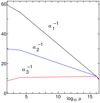
Figure 3: Behavior of gauge coupling constants $\alpha_{i}^{-1}$ ($i=1,2,3$) in the case of $M_{5}=10^{4}$ GeV and $M_{10}=10^{16}$ GeV. For simplicity, we have neglected the SUSY breaking effects at $\mu\sim 10^{3}$ GeV in this figure.

As seen in Table 2, we have many U(3) non-singlet fields in the present model, so that the model does not give an asymptotic free theory. The evolution of the U(3) family gauge coupling constant $\alpha_{F}(\mu)$ is given by

$$\frac{d}{d\log\mu}\alpha^{-1}_{F}(\mu)=\frac{1}{2\pi}\left(9-\frac{1}{2}\sum\ell(R)\right),$$

where $\ell(R)$ is an index of the representation $R$ of the group U(3). The sum $\sum\ell(R)$ is given by $\sum\ell(R)=6$ for $\mu<\Lambda_{U3}$ and $\sum\ell(R)=15+15$ for $\Lambda_{U3}<\mu<\Lambda_{GUT}$, where we do not consider contribution from $\bar{\bf 5}^{\prime\prime}+{\bf 5}^{\prime\prime}$ because they have masses of the order of $\Lambda_{GUT}$. We find that $\alpha_{F}(\mu)$ does not blow up even in the case of $\Lambda_{U3}=10^{3}$ GeV unless $\alpha_{F}(m_{Z})>0.033$. We show behavior of $\alpha_{F}(\mu)$ in a typical case with $\Lambda_{U3}=2$ TeV and $\alpha_{F}(m_{Z})=0.02$ in Fig.4.

Figure 4: Behavior of the inverse $\alpha_{F}^{-1}$ of the U(3) family gauge coupling constant in the case with $\Lambda_{U3}=2$ TeV and $\alpha_{F}(m_{Z})=0.02$.

We do not discuss the behaviors of gauge coupling constants above $\mu=\Lambda_{GUT}$ because we have no scenario at $\mu>\Lambda_{GUT}$ at present.

5. Concluding Remarks

In conclusion, we have investigated a possibility that a family gauge symmetry U(3) has a comparatively low energy scale by considering an SU(5) compatible yukawaon model with two family symmetries U(3)$\times$O(3). Since all of yukawaons are SU(5) singlets, the existence of the yukawaons do not affect the SU(5) GUT model, so that we can inherit the successful results in the SU(5) GUT. However, the purpose of the present model is not to discuss problems which are peculiar to the SU(5) GUT scenario. We optimistically consider that those problems will be resolved by considering further higher GUT groups (SO(10) or E₆, and so on) and/or an extra-dimension scenario.

In the present model, we have the following matter fields:

$$(\bar{\bf 5}_{i}+{\bf 10}_{\alpha}+{\bf 1}_{\alpha})+(\bar{\bf 5}^{\prime\prime}_{i}+{\bf 5}^{\prime\prime\,i})+(\bar{\bf 5}^{\prime}_{\alpha}+{\bf 5}^{\prime}_{\alpha})+({\bf 10}^{\prime}_{\alpha}+\overline{\bf 10}^{\prime}_{\alpha}),$$

where $i$ and $\alpha$ are indices of U(3) and O(3), respectively. The particles $(\bar{\bf 5}^{\prime\prime}_{i}+{\bf 5}^{\prime\prime\,i})$ and $(\overline{\bf 10}^{\prime}+{\bf 10}^{\prime})_{\alpha}$ have masses of the orders of $\Lambda_{GUT}\sim 10^{16}$ GeV, while $({\bf 5}^{\prime}+\bar{\bf 5}^{\prime})_{\alpha}$ have masses of the order of $10^{4}$ GeV. The U(3) family symmetry is broken at $\mu=\Lambda_{U3}\sim 10^{3}$ GeV.

The most notable result is that we have been able to consider a double seesaw mechanism for up-quark mass generation as shown in Fig.2 by introducing O(3) family symmetry. (If we consider U(3)$\times$U(3) family symmetries, we cannot obtain the effective Yukawa interaction (2.12).) As a result, the $Y_{d}$-$\hat{Y}_{u}$ corresponding has been improved as seen in Eq.(1.15). Also, by considering that the fundamental yukawaon $\Phi_{e}$ is transformed a triplet (doublet + singlet) of a permutation symmetry as defined in Eq.(3.3), our model without a cutoff $\Lambda$ can take more simple forms.

In this paper, we did not give numerical results on the basis of the present model, because the phenomenology is almost the same as the previous model [6]. Phenomenology for the family gauge bosons with the scale $10^{3}$ GeV will be given elsewhere.

Acknowledgments

The author would like to thank T. Yamashita for helpful conversations. The work is supported by JSPS (No. 21540266).

References

• [1] Y. Koide, Phys. Rev. D 71, 016010 (2005).
• [2] N Cabibbo, Phys. Rev. Lett. 10, 531 (1963); M. Kobauashi and T. Maskawa, Prog. Theor. Phys. 49, 652 (1973).
• [3] B. Pontecorvo, Zh. Eksp. Teor. Fiz. 33, 549 (1957)and 34, 247 (1957); Z. Maki, M. Nakagawa and S. Sakata, Prog. Theor. Phys. 28, 870 (1962).
• [4] Y. Koide, Phys. Rev. D 79, 033009 (2009).
• [5] C. D. Froggatt and H. B. Nelsen, Nucl. Phys. B 147, 277 (1979).
• [6] Y. Koide, Phys. Lett. B 680, 76 (2009).
• [7] H. Georgi and S. L. Glashow, Phys.Rev.Lett. 32, 438 (1974).
• [8] Y. Koide, arXiv: 1106.0971 [hep-ph].
• [9] Y. Sumino, Phys. Lett. B 671, 477 (2009); JHEP 0905, 075 (2009).
• [10] Y. Koide, Jour. Phys. G 38, 085004 (2011).
• [11] S. Dimopoulos and F. Wilczek, in The Unity of the Fundamental Interactions, Proceedings of the 19th Course of the International School of Subnuclear Physics, Erice, Italy, 1981, edited by A. Zichichi (Plenum Press, New York, 1983); M. Srednicki, Nucl. Phys. B202, 327 (1982).
• [12] S. Pakvasa and H. Sugawara, Phys. Lett. B 73, 61 (1978); H. Harari, H. Haut and J. Weyers, Phys. Lett. B 78, 459 (1978).
• [13] Particle Data Group, K. Nakamura, et al., J. Phys. G 37, 075021 (2010).
• [14] Z.-z. Xing, H. Zhang and S. Zhou, Phys. Rev. D 77, 113016 (2008). And also see, H. Fusaoka and Y. Koide, Phys. Rev. D 57, 3986 (1998).
• [15] Y. Koide, Y. Sumino and M. Yamanaka, Phys. Lett. B695, 279 (2011).