Environ centrality reveals the tendency of indirect effects to homogenize the functional importance of species in ecosystems

Abstract

Ecologists and conservation biologists need to identify the relative importance of species to make sound management decisions and effectively allocate scarce resources. We introduce a new method, termed environ centrality, to determine the relative importance of a species in an ecosystem network with respect to ecosystem energy–matter exchange. We demonstrate the uniqueness of environ centrality by comparing it to other common centrality metrics and then show its ecological significance. Specifically, we tested two hypotheses on a set of 50 empirically-based ecosystem network models. The first concerned the distribution of centrality in the community. We hypothesized that the functional importance of species would tend to be concentrated into a few dominant species followed by a group of species with lower, more even importance as is often seen in dominance–diversity curves. Second, we tested the systems ecology hypothesis that indirect relationships homogenize the functional importance of species in ecosystems. Our results support both hypotheses and highlight the importance of detritus and nutrient recyclers such as fungi and bacteria in generating the energy–matter flow in ecosystems. Our homogenization results suggest that indirect effects are important in part because they tend to even the importance of species in ecosystems. A core contribution of this work is that it creates a formal, mathematical method to quantify the importance species play in generating ecosystem activity by integrating direct, indirect, and boundary effects in ecological systems.

1 Introduction

Identifying the functional importance of species is a fundamental step in describing community and ecosystem structure and function. It is essential for ecologists, conservation biologists, and resource managers to understand species relative importance so that they can make informed management decisions and effectively allocate limited conservation resources. Rank-abundance curves (Whittaker, 1965) are a classic tool used to describe the biodiversity and relative importance of species in a community. This approach generally assumes that the importance of the species is proportional to its abundance or biomass. Alternative techniques include using functional measures like productivity in dominance–diversity curves (Whittaker, 1965), and more recent concepts such as network role equivalence (Luczkovich et al., 2003), keystone species (Power et al., 1996), ecosystem engineers (Lawton, 1994; Jones et al., 1994), and more generally the concept of foundational species (Dayton, 1972; Ellison et al., 2005). However, quantifying the relative functional importance of species embedded in their communities remains a challenging problem. In this paper, we introduce a new approach to quantifying the relative functional importance of species in ecosystem networks termed environ centrality. While species importance can be defined in a variety of ways, here we specifically focus on their importance for energy–matter distribution in communities. While we focus on ecosystems, the methods are generally applicable to any complex system of conservative fluxes modeled as a network.

One reason that the fundamental step of quantifying species functional importance has not been fully addressed is that indirect interactions complicate the assessment. Organisms are embedded in an intricate web of interactions and it is this tangled network of relationships that enables indirect influences to become significant components of ecological and evolutionary interactions (e.g. Patten, 1984; Wootton, 1994; Whitham et al., 2006; Bascompte and Jordano, 2007; Estrada and Bodin, 2008; Montoya et al., 2009; Keith et al., 2010). For example, Poulin et al. (2010) showed how invasive species can increase the prevalence and severity of disease in a community through trait-mediated indirect effects. Trophic cascades are one type of trophic indirect effect that can have large and unexpected impacts on ecosystems (Carpenter et al., 1985; Mooney et al., 2010). For example, Berger et al. (2008) found that where wolf populations were extripated, mesopredator populations like coyotes were released from predator control. This then resulted in a four fold decrease in the survival rate of pronghorn fawns, a coyote prey item. Thus, understanding the ecological and functional importance of species in their ecosystem requires understanding the full environment of direct and indirect influences.

Network models of ecosystems let ecologists quantify species importance and are a key tool for determining the importance of indirect influences that are distributed through these types of interactions (e.g. Bondavalli and Ulanowicz, 1999; Dame and Christian, 2006; Belgrano et al., 2005). In these models, network nodes represent species, groups of species, or abiotic resource pools. Although the nodes may be a species complex or non-living compartment of energy–matter, we generically refer to them as species throughout this paper for simplicity. Network links represent the flow of energy–matter from one node to another. These energy–matter flows can be created by several ecological processes including feeding, death, and excretion. This representation of complex ecosystem interactions lets ecologists apply mathematical and computational tools to learn more about the structure and function of ecosystems. These ecosystem networks can be represented by weighted and directed graphs so that a link not only implies a relationship between two nodes but it also indicates how much (weighted) energy–matter and from whom to whom (directed) the energy–matter is flowing.

Ecological Network Analyses (ENA) are a collection of quantitative methods that systematically asses information from a full, complex network description. There are several specific implementations of this concept, such as Ecopath (Christensen and Walters, 2004), Network Environ Analysis (Fath and Patten, 1999b; Fath and Borrett, 2006), EcoNet (Schramski et al., 2010), and NETWRK (Ulanowicz, 1986). ENA’s throughflow analysis mathematically partitions ecosystem energy–matter flow across boundary, direct, and indirect paths in the network (Fath and Patten, 1999b; Fath and Borrett, 2006; Schramski et al., 2010). This approach has been applied to analyze the structure and function of ecosystems. For example, Finn (1980) used the technique to characterize mineral cycling in the Hubbard Brook ecosystem. More recently, Borrett et al. (2006) and Schramski et al. (2006) investigated nitrogen cycling in the Neuse River Estuary, and Zhang et al. (2010) investigated the urban water metabolic system of Beijing. ENA lets scientist study the efferent and afferent holistic environments of species within a system boundary, which Patten termed environs (Patten, 1978).

Based on the development and application of ENA, systems ecologists have hypothesized that indirect energy–matter flows tend to dominate direct flows in ecosystems (Higashi and Patten, 1989; Jørgensen et al., 2007). Fath (2004) found support for this hypothesis in large ecosystem models generated from a community assembly type algorithm, Borrett et al. (2006) found supporting evidence for the hypothesis in 16 seasonal nitrogen cycling models for the Neuse River estuary, and Salas and Borrett (2011) found general support for the hypothesis in 50 empirically-based trophic ecosystem models. A consequence of these large indirect energy–matter flows is that resources tend to be more evenly distributed in the systems (Fath and Patten, 1999a; Borrett and Salas, 2010). Given this tendency, we hypothesized that indirect effects tend to homogenize the relative importance of the species, decreasing the relative influence any single species has on ecosystem functioning.

This paper has three main objectives. First, we introduce a new metric of functional importance based on the throughflow analysis of ENA and centrality concepts from social science. We contrast this measure with other existing centrality indexes to demonstrate its utility and uniqueness. Second, we use this measure to characterize the relative importance of species in 50 trophic ecosystem models. Third, we test two hypotheses regarding the functional organization of ecosystems. Based on previous community analysis, we first hypothesized that there will tend to be a “concentration of dominants” or functionally more important species and a “long tail” of species with a lower and more similar importance. We expected that the ecosystem dominants would be compartments like detritus, particulate organic matter, and bacteria because of their critical role in recirculating energy–matter and connecting the green and brown food webs (Wilkinson, 2006; Jordán et al., 2007). We further tested the hypothesis that indirect effects tend to homogenize the relative importance of species.

This paper is organized as follows. In the next section we introduce the centrality concept and describe its use and diversity. We then describe the ENA throughflow analysis that we use and introduce the environ centrality measure. Section 4 describes our analytical approach to testing our hypotheses and Section 5 describes our results. We conclude the paper by putting these results into a broader context.

2 Centrality

Centrality is a concept used by scientists studying complex systems that was initially developed by social scientists to quantify the importance of individuals in network models (Wasserman and Faust, 1994; Borgatti, 2005). Metrics based on this concept indicate how a node’s position in the network contributes to its structural or functional importance. There are multiple centrality metrics with varying characteristics (Wasserman and Faust, 1994; Borgatti and Everett, 2006), but many tend to be well correlated (Valente et al., 2008; Newman, 2006). Despite this correlation, differences between the measures can be useful. For example, degree centrality is based on the number of network edges directly touching a node and describes the local or proximate importance of the node. In contrast, eigenvector centrality describes the stable distribution of pathways (i.e. at long pathways) passing through the nodes, which provides a more global or whole network understanding of the nodes’ relative importance. These different measures have been well described in the literature, so here we focus on the ecological relevance of selected centrality measures.

There are several approaches to quantitatively describing ecosystem networks (Ulanowicz, 1986; Bersier et al., 2002). Several metrics commonly used to describe food webs such as link density and connectance (Dunne et al., 2002) are what Wasserman and Faust (1994) call group level indicators of centrality. Link density is the average node degree in the network. Connectance is link density proportional to the size of the network. Degree centrality, and thus link density and connectance, is a local centrality metric because it only considers the immediately adjacent neighborhood of connected nodes. Local centrality metrics may be a useful starting point for describing a food web, but they may not be the best descriptors of the organism’s importance in energy–matter transference because they assume the influence is restricted to a local neighborhood. Thus, they neglect the important indirect influences. From a trophic point of view, indirect effects become important in part because energy–matter is passed from one organism to another and may ultimately reenter the same organism through nutrient cycling, creating a well connected web of interactions (Allesina et al., 2005; Borrett et al., 2007).

Centrality metrics that incorporate indirect influences include betweenness centrality (Freeman, 1979), eigenvector centrality (Bonacich, 1972; Borgatti, 2005; Estrada and Bodin, 2008; Allesina and Pascual, 2009), and weighted topological importance (Bauer et al., 2010; Jordán et al., 2003). These centrality metrics are more appropriate for many ecological applications than those that only consider direct influences, but still have important limitations. Betweenness centrality considers the possible gatekeeper role that some nodes may play in the transfer of information, energy, and matter from two more distinct groups. While this metric can be useful, its focused on a particular type of bridging importance (Wasserman and Faust, 1994) and was not intended to provide a more general metric of the importance of a node. In trophic or biogeochemical network models, eigenvector centrality effectively quantifies the equilibrium distribution of energy–matter flowing through the nodes, thus considering the direct and indirect interactions. However, there are two potential problems with this measure for ecological networks. First, it ignores the contribution of the initial transient effects that maybe important in some contexts, especially systems in which the strength of interaction decreases rapidly with path length like ecosystems (Borrett et al., 2010). Second, it only considers the dominant eigenvector, which depending on the structure of the network may not be an adequate approximation of the transfer dynamics (Borgatti and Everett, 2006). Weighted topological importance quantifies the effect a species has on others in a community, which is great for understanding competition but does not provide information on how species contribute to global network properties such as total energy–matter throughflow. To address these limitations, we introduce environ centrality, which uses weighted information, integrates direct and indirect effects, describes how species contribute to global network measures, and captures the transient dynamics as well as the equilibrium effects.

3 Ecological Network Analysis

3.1 Throughflow Decomposition

As comprehensive summaries of ENA methodology exist (Ulanowicz, 1986; Fath and Borrett, 2006; Schramski et al., 2010), here we focus on the components of ENA necessary to calculate the centrality of species in ecosystem network models. We used the Network Environ Analysis Matlab^® function (Fath and Borrett, 2006) to implement these analyses.

Let a network model with $n$ nodes be represented by a matrix, $\mathbf{F}_{n\times n}=(f_{ij})$, which defines the quantity of energy–matter being transferred from node $j$ to node $i$. The structural component of $\mathbf{F}$ is the adjacency matrix, $\mathbf{A}=(a_{ij})$, in which a 1 indicates a direct connection from $j$ to $i$ and 0 indicates none. Energy–matter entering the system at node $i$ is denoted by $z_{i}$, whereas energy–matter leaving the system at node $j$ is $y_{j}$.

ENA uses this system data to determine several ecosystem properties. First, the total flow through a node is defined as throughflow, which can be input $T_{i}=z_{i}+\sum_{j=1}^{n}f_{ij}$ or output $T_{j}=\sum_{i=1}^{n}f_{ij}+y_{j}$ oriented. ENA typically assumes that the networks are at steady state (e.g., mass-balanced) so $T_{i}=T_{j}$. Second, we calculate the direct flow intensity matrix $\mathbf{G}$. We focus on the output oriented direct flow intensity matrix, which is calculated as $\mathbf{G}=(g_{ij})=f_{ij}/{T_{j}}$. Elements of $\mathbf{G}$ are unitless and represent the direct flow intensity from node $j$ to node $i$. Third, raising $\mathbf{G}$ to a power $m$, gives the flow intensity between two compartments over all paths of length $m$. The sum of flow intensities over all pathways in a network is defined as the integral flow matrix $\mathbf{N}$, which is

$$\mathbf{N}\equiv\sum_{m=0}^{\infty}{\mathbf{G}^{m}}=\underbrace{\mathbf{G}^{0}}_{\textrm{Boundary}}+\underbrace{\mathbf{G}^{1}}_{\textrm{Direct}}+\underbrace{\mathbf{G}^{2}+\ldots+\mathbf{G}^{m}+\ldots}_{\textrm{Indirect}}.$$ (1)

$\mathbf{N}$ quantifies the intensity of output oriented throughflow from $j$ to $i$ over all pathways in the network. Since ecological systems are thermodynamically open, the energy–matter must dissipate as path length increases causing the sum of flow intensities over all pathways to converge. Thus, we can use the identity $(\mathbf{I}-\mathbf{G})^{-1}$, where $\mathbf{I}=\mathbf{G}^{0}$ is the identity matrix, to find the exact values of $\mathbf{N}$.

Multiplying the integral matrix $\mathbf{N}$ by the input vector $\mathbf{z}$ returns the output oriented node throughflow $\mathbf{T}=\mathbf{Nz}$. This equation ensures that equation (1) is a true partition of flow and that the flow elements are not double counted. Total System Throughflow ($TST=\sum_{j=1}^{n}T_{j}$) is the sum of node throughflows and is a global measure of the total network activity or size of the system. Thus, the integral matrix shows how $TST$ is generated by species in an ecological network and incorporates energy–matter flux over all indirect pathways. Environ centrality is calculated from the integral flow matrix and quantifies the relative importance of species in creating total system activity.

3.2 Environ Centrality

Environ centrality is a measure based on the ENA output-oriented integral flow matrix, $\mathbf{N}$. We introduce three related environ centrality measures: input ($EC^{in}$), output ($EC^{out}$), and an average of the two ($AEC$). These are calculated as follows:

$$EC^{in} =\frac{\sum_{j=1}^{n}n_{ij}}{\sum_{i=1}^{n}\sum_{j=1}^{n}n_{ij}};$$

$$EC^{out} =\frac{\sum_{i=1}^{n}n_{ij}}{\sum_{i=1}^{n}\sum_{j=1}^{n}n_{ij}};\textrm{ and}$$

$$AEC =\frac{EC_{i}^{in}+EC_{j}^{out}}{2}.$$ (2)

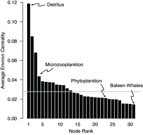
Figure 1: Rank $AEC$ curve of the Georges Bank Ecosystem network model. The grey line indicates the potential even distribution. Notice that the area under the curve sums to one.

$EC^{in}$ and $EC^{out}$ indicate the relative importance of species in generating ecosystem activity from an input or output direction, respectively. $AEC$ determines the relative importance of species in ecosystem models by averaging the input and output importance. Thus, $AEC$ quantifies the relative contribution of a node to the energy–matter exchange within a system. It is a global centrality measure of the functional importance of species because it incorporates direct and indirect pathways, weighting pathways by the amount of energy–matter flux intensity passing through a node. Further, it captures the transient dynamics as well as the equilibrium dynamics and describes how a species contributes to total system activity. Fig. 1 shows an example rank-order distribution of $AEC$ for the Georges Bank ecosystem (Link et al., 2008).

ENA is an Input–Output analysis in which it is possible to calculate output oriented and input oriented integral flow intensities (Fath and Borrett, 2006; Schramski et al., 2010). Thus, it is possible to calculate the $EC^{in}$, $EC^{out}$, and $AEC$ for both of these orientations. The interpretation of output and input oriented integral flow intensities differ. The output orientation looks forward in time and follows the direction of the network arrows. The input orientation looks backward through the network, against the arrow directions, to see where the flow has come from. Both orientations can be analytically useful independently and when jointly considered (Ulanowicz and Puccia, 1990; Schramski et al., 2006). As the purpose of this paper is to introduce environ centrality and illustrate its ecological significance, only the output oriented case is analyzed for simplicity. We expect the input oriented results to be similar, although the interpretation will differ.

4 Experimental Design

In this section we describe our experimental design to test our hypotheses. We first characterize the set of 50 empirically based ecosystem models we analyzed. We then explain our evaluation of the utility and uniqueness of $EC$. Finally, we describe our approach for determining species dominance and the centrality homogenization in 50 ecosystem networks.

4.1 Network Models

We calculated $AEC$ for 50 empirically-based network models of ecosystem energy–matter flows (Table 2). Borrett and Salas (2010) first assembled this data set to test the distinct systems ecology resource homogenization hypothesis. The collection is available from http://people.uncw.edu/borretts/research.html. Models were selected that spanned a range of sizes from smaller, highly aggregated systems comprising 4 nodes to larger, less aggregated systems comprising 125 nodes. Each network model traces trophic and non-trophic energy–matter transactions such as feeding, excretion, mortality, immigration and emigration and together represent 35 distinct ecosystems. To avoid a selection bias, all models discovered in the literature that were created to model a specific ecosystem and that included empirical data were included in the data set (see Salas and Borrett, 2011, for more details). To meet the ENA steady-state assumption, we balanced 15 of the 50 models using the AVG2 algorithm, which Allesina and Bondavalli (2003) demonstrated minimized balancing bias.

4.2 AEC Sensitivity and Uniqueness

Given the environ centrality metric, our first step was to evaluate its sensitivity and demonstrate its novelty. To illustrate its sensitivity, we compared $AEC$ values for four realizations of a hypothetical ecosystem flow network (Fig. 2). The four realizations vary in their distribution of flow amongst the five internal direct pathways. This is evident in the direct flow intensity matrices, $\mathbf{G}$, and the subsequent integral flow matrices, $\mathbf{N}$. The direct flow intensity values in the second realization are 10% of those in the first, which is a universal extensive change. The distribution of flow intensities is the same, but in the second realization the total magnitude is less. Realizations three and four have equal total flow intensities, but differ in how it is distributed. Thus, this is an example of an intensive change. Together, these realizations demonstrate $AEC$’s ability to capture both intensive and extensive network changes. In addition to $AEC$, we also examined the average eigenvector centrality $AEVC$ (Table 1) since these were likely to be the most similar centrality measures.

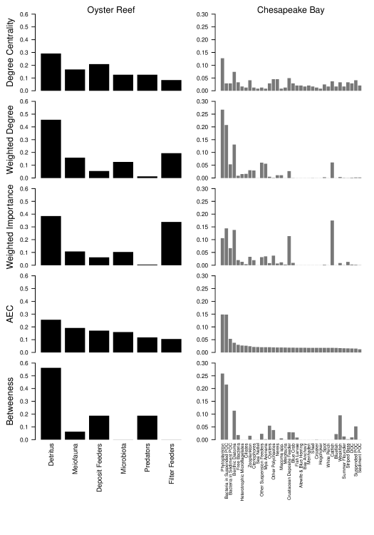
Figure 3: $DC$, $WD$, $WI$, $AEC$, and $BC$ distributions for Oyster Reef and Chesapeake Bay network models. Model nodes are ordered according to $AEC$ rank.

To show $AEC$’s uniqueness, we compared its results in two ecosystem models to five commonly used centrality metrics: degree centrality ($DC$), weighted degree centrality ($WD$), weighted topological importance ($WI$), and betweenness centrality ($BC$). The Oyster Reef and Chesapeake Bay models were selected as case studies to demonstrate the distributions of these five centrality metrics in empirical network models (Fig. 3). We calculated all metrics using common formulations (Table 1) and then normalized each set of scores by its sum (sensu Ruhnau, 2000), creating proportions to facilitate comparisons among the five metrics. In addition to the comparisons in Fig. 3, we compared $AEC$ and $AEVC$ for four network models; the Oyster Reef, Chesapeak Bay, Bothnian Bay, and Northern Benguela. Finally, we calculated the Spearman rank correlation of the $AEC$ and $AEVC$ in the 50 empirically based ecosystem models listed in Table 2. We focus on these two centrality measures because they are most likely to be similar because they are both global pathway centralities.

4.3 Dominance and Evenness

To address our hypothesis regarding the relative importance of species in ecosystems, we used the coefficient of variation ($CV$) to characterize the evenness of the $AEC$ distribution and to identify dominant species in 50 ecosystem models. Although there are multiple methods for quantifying variation, we chose $CV$ because it is a non-dimensional measure normalized to the mean values. This lets us compare the relative variation across systems, even if they differ in the number of species or $TST$. In addition, $CV$ is sensitive to distribution skew (Fraterrigo and Rusak, 2008), which we use to our advantage to identify dominant species.

We considered ecosystems with a $CV$ less than unity (1) to be low variance. To identify the dominant species, we ranked species according to their $AEC$ scores and calculated the $CV$ for the entire community. We then progressively removed the highest ranking species until the $CV$ of the remaining community $AEC$ was less than or equal to $0.5$. A $CV$ value of 0.5 is low enough to identify dominant species without being so low as to claim all species are dominant. It also identifies which species are responsible for the highest proportion of the variation in $EC$. All species removed before reaching the $CV$ threshold are classified as dominant species with respect to the ecosystem flux of energy–matter. Thus, this approach determines both the evenness of non-dominant species, and identifies the dominant species.

4.4 Homogenization and Indirect Effects

Our final hypothesis was that indirect flows would homogenize the relative importance of species in generating $TST$. We addressed this hypothesis by comparing the relative importance of species in the direct flows to those of the integral flows. Recall that equation 1 calculates the integral flow intensity matrix $\mathbf{N}$ that combines flow intensity over all boundary ($\mathbf{G}^{0}$), direct ($\mathbf{G}^{1}$), and indirect pathways ($\sum_{m=2}^{\infty}\mathbf{G}^{m}$). To find the relative importance of species from the perspective of the direct flows alone, we substituted $\mathbf{G}$ for $\mathbf{N}$ in equation 2 to calculate direct average environ centrality ($AEC^{direct}$). We then compared $AEC^{direct}$ to the integral average environ centrality ($AEC$) to test the homogenizing effect of indirect relationships on $AEC$.

As the integral matrix includes boundary, direct, and indirect flow intensities, it is possible that observed homogenization could be caused by the boundary input as well as the indirect flows. To isolate the effect of the indirect flows, we also compared the $AEC^{direct}$ to the $AEC$ calculated on $\mathbf{N}-\mathbf{G}^{0}$ instead of $\mathbf{N}$.

Homogenization of species importance was quantified by comparing the $CV$ of $AEC^{direct}$ and the $CV$ of $AEC$. We created a ratio of the two, $CV(AEC^{direct})/CV(AEC)$, such that when the ratio is greater than unity (1) it indicates that the $AEC$ is more evenly distributed than $AEC^{direct}$. Ratio values greater than unity indicate that indirect effects homogenize the importance of species in generating ecosystem activity.

5 Results

5.1 EC Sensitivity and Uniqueness

To establish the sensitivity of $AEC$ to both intensive and extensive changes, we applied it to four realizations of the hypothetical ecosystem model shown in Fig. 2. The $AEC$ distributions for the realizations are clearly different (Fig. 2D). In the first realization, the detritus box was more important and the importance of the primary producer was diminished. In the second realization in which the direct flow intensities were reduced by 90%, the $AEC$ values are much more similar. This is because the drop in flow intensities is then transmitted through the longer pathways, effectively discounting them. However, there is no difference between the $AEVC$ centrality distributions between realization one and two, demonstrating that eigenvector centrality is not sensitive to this extensive change.

Realizations three and four maintained the total magnitude of the network but have different distributions, which is an intensive change. The $AEC$ and $AEVC$ distributions between realization three and four are different, demonstrating that both metrics are sensitive to these intensive changes. In the third realization, one flux to the consumer compartment increased which caused it to become the second most central compartment. The detritus compartment also responded to the change, increasing its centrality from 0.26 to 0.30. For the fourth realization, the flux from detritivore to detritus increased, causing detritus to maintain its centrality from the previous realization at 0.30 and detritivores to increase its centrality to 0.30 as well. These four cases show that $AEC$ is sensitive enough to capture important differences between the model flow realizations, and specifically demonstrates its ability to capture both intensive and extensive changes to direct energy–matter flows.

The comparison of the four centrality metrics to $AEC$ in the Oyster reef and Chesapeake Bay ecosystem models (Fig. 3) shows the different structural and functional importance of the species within each network and illustrates the unique perspective of $AEC$. $DC$ highlights which species were most connected within the network topology (unweighted), yet was not always a predictor of which species would be most important in generating $TST$. There were several disparities between $DC$ and $AEC$ which show that being the most connected does not necessarily result in being a key species in generating $TST$. For example, the suspended particulate nutrient node from the Chesapeake Bay model has a greatly reduced ranking in $AEC$ despite having the second largest $DC$. $WD$ had similar mismatches with $AEC$, and demonstrates that high or low magnitudes of direct flows are not always indicative of overall importance in generating ecosystem activity. In both models, $WI$ consistently placed primary producers and herbivores (i.e. filter feeders, phytoplankton, and zooplankton) as species with the highest effect on others, yet these species ranked low in $AEC$. The $BC$ distribution was the most distinct centrality metric.

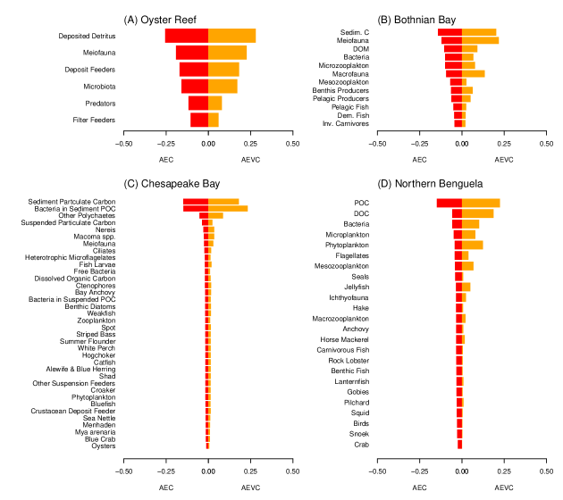
Figure 4: Comparison of the average environ centrality ($AEC$) and average eigenvector centralities ($AEVC$) for the (A) Oyster Reef (B) Bothnian Bay (C) Chesapeake Bay and (D) Northern Benguela ecosystem models. The nodes have been ordered in ascending order of the average environ centrality to facilitate comparison. The $AEC$ distributions were multiplied by -1 for plotting convenience.

Average eigenvector centrality should be the most similar to average environ centrality because they are both global centrality measures related to pathways or energy–matter flow; however, we see from Fig. 2 that they can differ. Fig. 4 further illustrates differences between $AEVC$ and $AEC$. It shows both types of centralities for four cases: the Oyster Reef and Chesapeake Bay models used in Fig. 3 and the Bothnian Bay and Northern Benguela ecosystem models. The centralities indicate a difference of the rank-order importance of the nodes for all models except the Oyster Reef. For example, $AEC$ suggests that Bacteria, DOM, Mesozooplankton, and Microzooplankton have a larger functional importance in the Bothnian Bay ecosystem than is suggested by the eigenvector centrality (Fig. 4B). In contrast, eigenvector centrality indicates a very dominant importance of Meiofauna, Sediment carbon, and Macrofauna. The two centralities also show a different rank importance of the nodes in the Northern Benguela ecosystem model. From the $AEC$ perspective, POC has a dominant importance, while most of the other species have very similar centralities. Variation in $AEVC$ is larger in all models, including Oyster Reef where the rank importance are the same. One interesting difference is the diminished importance of Seals suggested by $AEVC$ for Fig. 4D). Additionally, $AEVC$ ranks bacteria in sediment POC as more important than Sediment Particulate Carbon in Fig. 4C while the $AEC$ values are nearly the same.

To generalize our analysis, we calculated the Spearman rank correlation between $AEC$ and $AEVC$ for the 50 ecosystem network models (Table 2). These correlations ranged from 0.2 to 1 and had a median value of 0.92. As we expected, this suggests that these two centrality measures are typically, but not always, similar. Our case studies in Fig. 4 highlight how these small correlation differences can be ecologically meaningful.

5.2 Dominance and Evenness

Rank $AEC$ curves provide a tool to visualize the relative importance of species (Fig. 1). The $AEC$ distribution of the Georges Bank illustrates the tendency for a few nodes to have high $AEC$ with most having relatively lower and even $AEC$ values. $AEC$ variation in the ecosystem models we analyzed was generally low (Table 3). Twelve of the models have a $CV(AEC)$ less than $0.5$ and 30 of the models have a $CV(AEC)$ between $0.5$ and unity. However, eight of the models exhibit more variability with CV values larger than unity. In the models with a CV larger than $0.5$, no more than three dominant species had to be removed before the $CV$ of the remaining species fell below $0.5$ (Table 3). The median number of dominants was two. As expected, detritus and detrital recyclers are predominantly responsible for generating $TST$ in most ecosystems, with water flagellates being the only non-detrital or bacterial species to rank as dominant $AEC$ contributors.

The second hypothesis was that sub-dominant species would have a more even distribution of importance. In Fig. 1, the first two species were considered dominant species and the $CV$ score for the whole ecosystem was 0.68. However, once the dominants were removed the $CV$ score of the remaining species was $0.41$ suggesting less variation in the importance of the remaining species. Table 3 identifies the $CV$ value of the entire community, as well as the community without the dominant species for all 50 ecosystem models. After the dominant species were removed, the $AEC$ scores were relatively even, with an average $CV$ score of $0.38$. This indicates that the standard deviation was only 38% the magnitude of the mean. All the networks support our hypothesis that the importance of sub-dominant species would be relatively even.

5.3 Homogenization and Indirect Effects

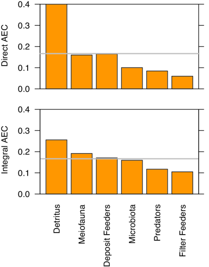
Figure 5: Comparing the direct and integral (direct, boundary, and indirect) $AEC$ distributions. The gray line represents the value if each node had the same centrality.

The comparison of direct and integral $AEC$ in the Oyster Reef model (Fig. 5) illustrates how the relative importance of species in generating $TST$ can become more similar when indirect flows are considered. Fig. 6 shows that this is a general trend as 49 of the 50 network models (98%) exhibited less variation in $AEC$ when indirect flows were considered. The EMS estuary was the only network to not meet our expectation. Furthermore, when boundary effects were excluded from our analysis, 33 of 50 ecosystems (66%) exhibited homogenized importance due to indirect effects alone. Thus, indirect effects appear to homogenize the importance of species in ecosystems.

6 Discussion

6.1 Ecological Significance

Our results make two ecologically significant contributions. First, $AEC$ is a novel way to quantify the relative functional importance of species or functional groups in an ecosystem with respect to the global energy–matter exchange of a network. It is sensitive to both extensive and intensive changes, and incorporates indirect effects. With this metric, we gain new insight into the distribution of species contribution to the total system activity. Second, the results highlight another critical consequence of indirect interactions in ecosystems; they tend to make species’ functional importance more similar. If this pattern holds generally, it has important implications for conservation biology which we discuss below.

Our results support the hypothesis that ecosystems are comprised of a few functionally dominant species and a larger set of species with relatively similar functional importance. The smaller $CV$ values for the remaining community after the dominants are excluded demonstrate that the top ranked species are responsible for a majority of the variation in $AEC$ and that most species in ecosystems have relatively low and even centralities. This is further evidence for the general dominance–diversity community patterns initially described by Whittaker (1965).

The second hypothesis this paper tested concerned the effect of indirect flows on the species’ environ centralities. Our results support the hypothesis that indirect effects tend to even the functional importance of species. Indirect flows alone homogenized the importance of species in 66% of the ecosystem networks analyzed. The empirical literature is rich with examples of indirect relationships driving ecosystem reactions (Berger et al., 2008; Bondavalli and Ulanowicz, 1999; Carpenter et al., 1985; Wootton, 1994) and our theoretical analysis provides evidence for another important consequence of indirect effects.

The EMS estuary was the only network in which the integral centrality $AEC$ was not more even than the direct environ centrality $AEC^{Direct}$. This could be because of the extreme dominant centrality of the sediment POC in this model. After removing sediment POC from the $AEC$ variation analysis, the $CV$ declined 70% which was one of the largest percent drops in variation. It was also one of the few ecosystems to have a $CV(AEC)$ that was greater than unity.

Collectively, our homogenization results support the trend towards whole ecosystem management for conservation biology. Although a few species may have a dominant functional importance, most species are contributing in similar ways. This could be interpreted as suggesting that losing the non-dominant species would have less significant impacts on the system, but this misses a fundamental aspect of the results. The homogenization of the species centralities is a consequence of the indirect interactions that are distributed across the network of relationships. This depends on the existing species and their pattern of direct and indirect connections. Thus these results show that preserving the intact network is critical to maintain current ecosystem total energy–matter throughflow.

6.2 Centrality metric comparisons

Our comparison of centrality metrics in Fig. 3 highlights the differences and similarities between these five metrics. In the case of $WD$ and $WI$, both metrics are calculated from the same matrix $\mathbf{F}$, but differ by the anchoring metric (i.e. sum of energy–matter entering a node versus total energy–matter flowing in the network) and the length of the pathways considered. This may explain the similarities between $WD$ and $WI$ as seen in the Oyster Reef model.

Average eigenvector centrality should be the most similar to average environ centrality because they are both global centrality measures related to pathways or flow. However, our results show that these centrality measures can be quite different. The results of the hypothetical ecosystem model are most instructive (Fig. 2). The first and second model realizations whose direct flow intensity distributions are the same have the same $AEVC$ distributions. The large drop in direct transfer efficiencies does not affect the equilibrium distribution of flows, thus the eigenvector centralities remain the same. This is unlike $AEC$ which does respond to the drop in transfer efficiency because it captures the transient flow dynamics as well as the equilibrium distribution. This demonstrates the ability of $AEC$ to capture extensive changes that $AEVC$ does not. Both $AEC$ and $AEVC$ capture differences between realizations three and four, demonstrating that both are able to capture intensive changes to direct energy–matter flow. Although $AEC$ and $AEVC$ are well correlated, most centrality metrics tend to be well correlated (Valente et al., 2008; Newman, 2006), and small differences between metrics can be biologically important (see Fig. 4).

Alternative centrality measures have different values. We do not expect one to be the universally correct analytical choice. If the goal is to understand the relative importance of nodes in generating the total system activity of a network model of conservative flows, the evidence presented here suggests that $AEC$ is a good choice.

6.3 Future work and limitations

Despite the limitations of the set of ecosystem network models (e.g. relatively few model authors, only 35 distinct ecosystems, some very small models $n<5$, mass–balanced assumption), the consistency of the results suggests they are robust to model error. To verify the generality of these results, this data set can be extended to include biogeochemically-based networks that may reflect different aspects of ecosystem organization (Borrett et al., 2010) as more models become available. Our preliminary analysis suggest that these results may hold true for biogeochemically–based networks, but this remains a testable hypothesis.

One important direction for future research is clarifying the relationship between alternative methods for quantifying the “importance” and “effects” species have on one another (Ulanowicz and Puccia, 1990; Jordán et al., 2003; Schramski et al., 2006; Bauer et al., 2010). For example, Schramski et al.’s (2006) measure of distributed control among species in a network is calculated using the input and output oriented integral flow matrices. There are some clear conceptual differences, but since the underlying data and analytical goals are the same we expect there to be an interesting relationship between $AEC$ and distributed control. Another possible comparison would be to calculate $WI$ beyond path lengths of 10 to see how longer indirect relationships effect this centrality metric in an ENA framework.

6.4 Summary

This work makes three core contributions to ecology. First, we introduce a formal method called environ centrality to quantify the relative importance of species in generating ecosystem activity. This metric builds on the centrality concept from the social sciences and Patten’s environ concept, and can be considered in a manner similar to rank-abundance curves familiar to many ecologists. The main ecological advantages of environ centrality are that it is the only metric to date to include all direct and indirect effects of a weighted ecosystem network model, it is simple to calculate in the ENA framework, and it should easily apply to network models of flow in other types of complex systems. Further, it is sensitive to both extensive and intensive changes to direct flow intensities, and does not ignore the sometimes important transient dynamics like eigenvector centrality does. Second, we applied environ centrality to find evidence that support the hypothesis that ecosystems are comprised of both a few functionally dominant species and a larger group of species with more similar importance. Our results expose the central importance of detritus and decomposer species like bacteria and fungi in generating carbon throughflow activity in ecosystems. This result is not surprising, but it supports our claim that environ centrality is a useful ecological measure. Third, this work shows that indirect effects tend to homogenize the functional importance of species. This is further evidence of the important consequences that different types of indirect effects can have in complex systems like ecosystems.

7 Acknowledgments

This research and manuscript benefited form critiques by Z. Long, A. Stapleton, M. Freeze, A. Salas, D. Hines, and M. Lau. Two anonymous reviewers also greatly improved the readability and scholarship of this manuscript. We would also like to thank D. Baird, R.R. Christian, J. Link, A. L. J. Miehls, U. Sharler, and R. E. Ulanowicz for sharing many of their ecosystem models with us. Lastly, we gratefully acknowledge financial support from UNCW and NSF DEB-1020944 (SRB), the NOAA Ernest F. Hollings Scholarship and the UNCW Center for Support of Undergraduate Research and Fellowship (SLF).

Table 1: Formulas and references for centrality indices compared in this paper

Metric	Symbol	Formula	Citation
Degree Centrality	$DC$	$(\sum_{i=1}^{n}a_{ij}+\sum_{j=1}^{n}a_{ij})/2$	Freeman (1979)
Weighted Degree	$WD$	$(\sum_{i=1}^{n}f_{ij}+\sum_{j=1}^{n}f_{ij})/2$	Freeman (1979)
Betweenness Centrality†	$BC$	$2\sum_{j<k;i\neq j}\frac{h_{jk}i/h_{jk}}{(n-1)(n-2)}$ $h_{jk}$	Freeman (1979)
Weighted Importance	$WI$	$\sum_{k=1}^{m}\frac{\sum_{i=1}^{n}(\frac{f_{ij}}{\sum_{j=1}^{n}f_{ij}})^{m}}{m}$	Jordán et al. (2003); Bauer et al. (2010)
Eigenvector Centrality‡	$EVC$	$(v+w)/2$	Bonacich (1972)
Environ Centrality	$AEC$	$(EC_{j}^{in}+EC_{j}^{out})/2$

^† $h_{jk}i$ represents the number of shortest paths between node $j$ and $k$ that pass through node $i$. ^‡ $v$ and $w$ are the right and left hand eigenvectors of the dominant eigen value respectively.

Table 2: Fifty empirically-based trophic ecosystem network models.

 

Model	units	$n^{\dagger}$	$C^{\dagger}$	$TST^{\dagger}$	$FCI^{\dagger}$	Source
Lake Findley	gC m-2 yr-1	4	0.38	51	0.30	Richey et al. (1978)
Mirror Lake	gC m-2 yr-1	5	0.36	218	0.32	Richey et al. (1978)
Lake Wingra	gC m-2 yr-1	5	0.40	1,517	0.40	Richey et al. (1978)
Marion Lake	gC m-2 yr-1	5	0.36	243	0.31	Richey et al. (1978)
Cone Springs	kcal m-2 yr-1	5	0.32	30,626	0.09	Tilly (1968)
Silver Springs	kcal m-2 yr-1	5	0.28	29,175	0.00	Odum (1957)
English Channel	kcal m-2 yr-1	6	0.25	2,280	0.00	Brylinsky (1972)
Oyster Reef	kcal m-2 yr-1	6	0.33	84	0.11	Dame and Patten (1981)
Somme Estuary	mgC m-2 d-1	9	0.30	2,035	0.14	Rybarczyk et al. (2003)
Bothnian Bay	gC m-2 yr-1	12	0.22	130	0.18	Sandberg et al. (2000)
Bothnian Sea	gC m-2 yr-1	12	0.24	458	0.27	Sandberg et al. (2000)
Ythan Estuary	gC m-2 yr-1	13	0.23	4,181	0.24	Baird and Milne (1981)
Baltic Sea	mgC m-2 d-1	15	0.17	1,974	0.13	Baird et al. (1991)
Ems Estuary	mgC m-2 d-1	15	0.19	1,019	0.32	Baird et al. (1991)
Swarkops Estuary	mgC m-2 d-1	15	0.17	13,996	0.47	Baird et al. (1991)
Southern Benguela Upwelling	mgC m-2 d-1	16	0.23	1,774	0.19	Baird et al. (1991)
Peruvian Upwelling	mgC m-2 d-1	16	0.22	33,496	0.04	Baird et al. (1991)
Crystal River (control)	mgC m-2 d-1	21	0.19	15,063	0.07	Ulanowicz (1986)
Crystal River (thermal)	mgC m-2 d-1	21	0.14	12,032	0.09	Ulanowicz (1986)
Charca de Maspalomas Lagoon	mgC m-2 d-1	21	0.13	6,010,331	0.18	Almunia et al. (1999)
Northern Benguela Upwelling	mgC m-2 d-1	24	0.21	6,608	0.05	Heymans and Baird (2000)
Neuse Estuary (early summer 1997)	mgC m-2 d-1	30	0.09	13,826	0.12	Baird et al. (2004b)
Neuse Estuary (late summer 1997)	mgC m-2 d-1	30	0.11	13,038	0.13	Baird et al. (2004b)
Neuse Estuary (early summer 1998)	mgC m-2 d-1	30	0.09	14,025	0.12	Baird et al. (2004b)
Neuse Estuary (late summer 1998)	mgC m-2 d-1	30	0.10	15,031	0.11	Baird et al. (2004b)
Gulf of Maine	g ww m-2 yr-1	31	0.35	18,382	0.15	Link et al. (2008)
Georges Bank	g ww m-2 yr-1	31	0.35	16,890	0.18	Link et al. (2008)
Middle Atlantic Bight	g ww m-2 yr-1	32	0.37	17,917	0.18	Link et al. (2008)
Narragansett Bay	mgC m-2 yr-1	32	0.15	3,917,246	0.51	Monaco and Ulanowicz (1997)
Southern New England Bight	g ww m-2 yr-1	33	0.03	17,597	0.16	Link et al. (2008)
Chesapeake Bay	mgC m-2 yr-1	36	0.09	3,227,453	0.19	Baird and Ulanowicz (1989)
St. Marks Seagrass, site 1 (Jan)	mgC m-2 d-1	51	0.08	1,316	0.13	Baird et al. (1998)
St. Marks Seagrass, site 1 (Feb)	mgC m-2 d-1	51	0.08	1,591	0.11	Baird et al. (1998)
St. Marks Seagrass, site 2 (Jan)	mgC m-2 d-1	51	0.07	1,383	0.09	Baird et al. (1998)
St. Marks Seagrass, site 2 (Feb)	mgC m-2 d-1	51	0.08	1,921	0.08	Baird et al. (1998)
St. Marks Seagrass, site 3 (Jan)	mgC m-2 d-1	51	0.05	12,651	0.01	Baird et al. (1998)
St. Marks Seagrass, site 4 (Feb)	mgC m-2 d-1	51	0.08	2,865	0.04	Baird et al. (1998)
Sylt-Rømø Bight	mgC m-2 d-1	59	0.08	1,353,406	0.09	Baird et al. (2004a)
Graminoids (wet)	gC m-2 yr-1	66	0.18	13,677	0.02	Ulanowicz et al. (2000)
Graminoids (dry)	gC m-2 yr-1	66	0.18	7,520	0.04	Ulanowicz et al. (2000)
Cypress (wet)	gC m-2 yr-1	68	0.12	2,572	0.04	Ulanowicz et al. (1997)
Cypress (dry)	gC m-2 yr-1	68	0.12	1,918	0.04	Ulanowicz et al. (1997)
Lake Oneida (pre-ZM)	gC m-2 yr-1	74	0.22	1,638	$<0.01$	Miehls et al. (2009a)
Lake Quinte (pre-ZM)	gC m-2 yr-1	74	0.21	1,467	$<0.01$	Miehls et al. (2009b)
Lake Oneida (post-ZM)	gC m-2 yr-1	76	0.22	1,365	$<0.01$	Miehls et al. (2009a)
Lake Quinte (post-ZM)	gC m-2 yr-1	80	0.21	1,925	$0.01$	Miehls et al. (2009b)
Mangroves (wet)	gC m-2 yr-1	94	0.15	3,272	0.10	Ulanowicz et al. (1999)
Mangroves (dry)	gC m-2 yr-1	94	0.15	3,266	0.10	Ulanowicz et al. (1999)
Florida Bay (wet)	mgC m-2 yr-1	125	0.12	2,721	0.14	Ulanowicz et al. (1998)
Florida Bay (dry)	mgC m-2 yr-1	125	0.13	1,779	0.08	Ulanowicz et al. (1998)

  ^† $n$ is the number of nodes in the network model, $C=L/n^{2}$ is the model connectance when $L$ is the number of direct links or energy–matter transfers, $TST=\sum\sum{f_{ij}}+\sum{z_{i}}$ is the total system throughflow, and $FCI$ is the Finn Cycling Index (Finn, 1980).

Table 3: Dominate species and functional variation in 50 ecosystem network models

Model	CV(AEC)	CV(R-AEC)†	# Dominants	Dominant Identity
Lake Findley	0.48	0.48	0
Mirror Lake	0.51	0.17	2	Sediment, Benthos
Lake Wingra	0.43	0.43	0
Marion Lake	0.53	0.14	2	Sediment, Benthos
Cone Springs	0.23	0.23	0
Silver Springs	0.11	0.11	0
English Channel	0.16	0.16	0
Oyster Reef	0.33	0.33	0
Somme Estuary	0.58	0.18	1	POM
Bothnian Bay	0.34	0.34	0
Bothnian Sea	0.46	0.46	0
Ythan Estuary	0.50	0.50	0
Baltic Sea	0.40	0.40	0
Ems Estuary	1.03	0.31	1	Sediment POC
Swarkops Estuary	0.97	0.30	1	Sediment POC
Southern Benguela Upwelling	0.58	0.26	1	Suspended POC
Peruvian Upwelling	0.41	0.41	0
Crystal River (control)	0.56	0.27	1	Detritus
Crystal River (thermal)	0.61	0.30	1	Detritus
Charca de Maspalomas Lagoon	0.70	0.40	1	Sedimented POC
Northern Benguela Upwelling	0.58	0.23	1	POC
Neuse Estuary (early summer 1997)	0.79	0.43	2	Sediment POC, Sediment bacteria
Neuse Estuary (late summer 1997)	0.83	0.37	2	Sediment POC, Sediment bacteria
Neuse Estuary (early summer 1998)	0.80	0.44	2	Sediment POC, Sediment bacteria
Neuse Estuary (late summer 1998)	0.81	0.41	2	Sediment POC, Sediment bacteria
Gulf of Maine	0.65	0.41	2	Detritus/POC, Other Macrobenthos
Georges Bank	0.68	0.41	2	Detritus/POC, Other Macrobenthos
Middle Atlantic Bight	0.73	0.45	2	Detritus/POC, Other Macrobenthos
Narragansett Bay	1.34	0.39	3	Detritus/POC, Sediment POC Bacteria, Pelagic Bacteria
Southern New England Bight	0.68	0.49	1	Detritus/POC
Chesapeake Bay	1.10	0.36	2	Sedimented POC, Bacteria in Sediment (POC)
St. Marks Seagrass, site 1 (Jan.)	1.00	0.38	2	Sediment POC, Benthic Bacteria
St. Marks Seagrass, site 1 (Feb.)	0.94	0.42	2	Sediment POC, Benthic Bacteria
St. Marks Seagrass, site 2 (Jan.)	0.86	0.34	2	Sediment POC, Benthic Bacteria
St. Marks Seagrass, site 2 (Feb.)	0.86	0.35	2	Sediment POC, Benthic Bacteria
St. Marks Seagrass, site 3 (Jan.)	0.60	0.27	1	Sediment POC
St. Marks Seagrass, site 4 (Feb.)	0.75	0.34	1	Sediment POC
Sylt-Rømø Bight	1.17	0.44	1	Sediment POC
Graminoids (wet)	0.98	0.18	2	Sediment Carbon, Refractory Detritus
Graminoids (dry)	1.00	0.28	2	Sediment Carbon, Refractory Detritus
Cypress (wet)	0.89	0.49	3	Liable Detritus, Living Sediment, Vertebrate Detritus
Cypress (dry)	0.85	0.50	3	Vertebrate Detritus, Liable Detritus, Living Sediment
Lake Oneida (pre-ZM)	0.49	0.49	0
Lake Quinte (pre-ZM)	0.62	0.28	1	Sedimented Detritus
Lake Oneida (post-ZM)	0.49	0.49	0
Lake Quinte (post-ZM)	0.78	0.29	1	Sedimented Detritus
Mangroves (wet)	1.17	0.35	3	Sediment Carbon, Sediment bacteria, POC
Mangroves (dry)	1.19	0.35	3	Sediment Carbon, Sediment bacteria, POC
Florida Bay (wet)	1.43	0.46	3	Water POC, Benthic POC, Water Flagellates
Florida Bay (dry)	1.40	0.36	3	Water POC, Benthic POC, Water Flagellates

 

^† CV(R-AEC) represents the $CV$ of $AEC$ scores for all species remaining after dominates have been removed.

Figure 2: Example of average environ centralities ($AEC$) in four realizations of a hypothetical ecosystem model. (A) Model structure, (B) four mass balanced realizations of the direct flow intensity matrices, $\mathbf{G}$, for the model, (C) corresponding integral flow matrices, $\mathbf{N}$, (D) $AEC$ distributions, and (E) average eigenvector centralities $AEVC$. Notice that flow is from column $j$ to row $i$ in the matrices. When column sums of $\mathbf{G}$ do not equal 1, the remaining portion of flow is lost as exports or respiration.

Figure 6: $CV$ ratios quantifying the homogenization of roles in $AEC$ when compared to $AEC^{direct}$. Bars surpassing the vertical line at 1 represent ecosystems which exhibit centrality homogenization from indirect effects.

References

- Allesina et al. (2005) Allesina S, Bodini A, Bondavalli C. Ecological subsystems via graph theory: The role of strongly connected components. Oikos 2005;110:164–76.
- Allesina and Bondavalli (2003) Allesina S, Bondavalli C. Steady state of ecosystem flow networks: A comparison between balancing procedures. Ecological Modelling 2003;165:221–9.
- Allesina and Pascual (2009) Allesina S, Pascual M. Googling food webs: Can an eigenvector measure species’ importance for coextinctions? PLoS Computational Biology 2009;5:1175–7.
- Almunia et al. (1999) Almunia J, Basterretxea G, Aistegui J, Ulanowicz RE. Benthic–pelagic switching in a coastal subtropical lagoon. Estuarine Coastal and Shelf Science 1999;49:221–32.
- Baird et al. (2004a) Baird D, Asmus H, Asmus R. Energy flow of a boreal intertidal ecosystem, the Sylt-Rømø Bight. Marine Ecology Progress Series 2004a;279:45–61.
- Baird et al. (2004b) Baird D, Christian RR, Peterson CH, Johnson GA. Consequences of hypoxia on estuarine ecosystem function: Energy diversion from consumers to microbes. Ecological Applications 2004b;14:805–22.
- Baird et al. (1998) Baird D, Luczkovich J, Christian RR. Assessment of spatial and temporal variability in ecosystem attributes of the St Marks National Wildlife Refuge, Apalachee Bay, Florida. Estuarine Coastal and Shelf Science 1998;47:329–49.
- Baird et al. (1991) Baird D, McGlade JM, Ulanowicz RE. The comparative ecology of six marine ecosystems. Philosophical Transactions of the Royal Society of London Series B-Biological Sciences 1991;333:15–29.
- Baird and Milne (1981) Baird D, Milne H. Energy flow in the Ythan Estuary, Aberdeenshire, Scotland. Estuarine Coastal and Shelf Science 1981;13:455–72.
- Baird and Ulanowicz (1989) Baird D, Ulanowicz RE. The seasonal dynamics of the Chesapeake Bay ecosystem. Ecological Monographs 1989;59:329–64.
- Bascompte and Jordano (2007) Bascompte J, Jordano P. Plant-animal mutualistic networks: The architecture of biodiversity. Annual Reviews of Ecology and Systematics 2007;38:567–93.
- Bauer et al. (2010) Bauer B, Jordán F, Podani J. Node centrality indices in food webs: Rank orders versus distributions. Ecological Complexity 2010;7:471–7.
- Belgrano et al. (2005) Belgrano A, Scharler UM, Dunne J, Ulanowicz RE. Aquatic Food Webs: An Ecosystem Approach. New York, NY.: Oxford University Press, 2005.
- Berger et al. (2008) Berger KM, Gese EM, Berger J. Indirect effects and traditional trophic cascades: A test involving wolves, coyotes, and pronghorn. Ecology 2008;89:818–28.
- Bersier et al. (2002) Bersier LF, Bnasek-Richter C, Cattin MF. Quantitative descriptors of food-web matrices. Ecology 2002;83:2394–407
- Bonacich (1972) Bonacich P. Factoring and weighting approaches to clique identification. Journal of Mathematical Sociology 1972;2:113–20.
- Bondavalli and Ulanowicz (1999) Bondavalli C, Ulanowicz RE. Unexpected effects of predators upon their prey: The case of the American alligator. Ecosystems 1999;2:49–63.
- Borgatti (2005) Borgatti SP. Centrality and network flow. Social Networks 2005;27:55–71.
- Borgatti and Everett (2006) Borgatti SP, Everett MG. A graph-theoretic perspective on centrality. Social Networks 2006;28:466–84.
- Borrett et al. (2007) Borrett SR, Fath BD, Patten BC. Functional integration of ecological networks through pathway proliferation. Journal of Theoretical Biology 2007;245:98–111.
- Borrett and Salas (2010) Borrett SR, Salas AK. Evidence for resource homogenization in 50 trophic ecosystem networks. Ecological Modelling 2010;221:1710–6.
- Borrett et al. (2010) Borrett SR, Whipple SJ, Patten BC. Rapid development of indirect effects in ecological networks. Oikos 2010;119:1136–48.
- Borrett et al. (2006) Borrett SR, Whipple SJ, Patten BC, Christian RR. Indirect effects and distributed control in ecosystems 3. Temporal variability of indirect effects in a seven-compartment model of nitrogen flow in the Neuse River Estuary (USA)—time series analysis. Ecological Modelling 2006;194:178–88.
- Brylinsky (1972) Brylinsky M. Steady-state sensitivity analysis of energy flow in a marine ecosystem. In: Patten BC, editor. Systems analysis and simulation in ecology. Academic Press; volume Vol.2; 1972. p. 81–101.
- Carpenter et al. (1985) Carpenter SR, Kitchell JF, Hodgson JR. Cascading trophic interactions and lake productivity: Fish predation and herbivory can regulate lake ecosystems. Bioscience 1985;35:634–9.
- Christensen and Walters (2004) Christensen V, Walters CJ. Ecopath with Ecosim: Methods, capabilities and limitations. Ecological Modelling 2004;172:109–39.
- Dame and Christian (2006) Dame JK, Christian RR. Uncertainty and the use of network analysis for ecosystem-based fishery management. Fisheries 2006;31:331–41.
- Dame and Patten (1981) Dame RF, Patten BC. Analysis of energy flows in an intertidal oyster reef. Marine Ecology Progress Series 1981;5:115–24.
- Dayton (1972) Dayton PK. Toward an understanding of community resilience and the potential effects of enrichments to the benthos at McMurdo Sound, Antarctica. In: Parker E, editor. Proceedings of the colloquium on conservation problems in Antarctica. Lawrence, KS: Allen Press; 1972.
- Dunne et al. (2002) Dunne JA, Williams RJ, Martinez ND. Food-web structure and network theory: The role of connectance and size. Proc. Nat. Acad. Sci. 2002;99:12917.
- Ellison et al. (2005) Ellison A, Bank M, Clinton B, Colburn E, Elliott K, Ford C, Foster D, Kloeppel B, Knoepp J, Lovett G, et al. Loss of foundation species: consequences for the structure and dynamics of forested ecosystems. Frontiers in Ecology and the Environment 2005;3(9):479–86.
- Estrada and Bodin (2008) Estrada E, Bodin O. Using network centrality measures to managae landscape connectivity. Ecological Applications 2008;18(7):1810–25.
- Fath (2004) Fath BD. Network analysis applied to large-scale cyber-ecosystems. Ecological Modelling 2004;171:329–37.
- Fath and Borrett (2006) Fath BD, Borrett SR. A Matlab© function for network environ analysis. Environmental Modelling & Software 2006;21:375–405.
- Fath and Patten (1999a) Fath BD, Patten BC. Quantifying resource homogenization using network flow analysis. Ecological Modelling 1999a;107:193–205.
- Fath and Patten (1999b) Fath BD, Patten BC. Review of the foundations of network environ analysis. Ecosystems 1999b;2:167–79.
- Finn (1980) Finn JT. Flow analysis of models of the Hubbard Brook ecosystem. Ecology 1980;61:562–71.
- Fraterrigo and Rusak (2008) Fraterrigo JM, Rusak JA. Disturbance-driven changes in the variability of ecological patterns and processes. Ecology Letters 2008;11:756–70.
- Freeman (1979) Freeman LC. Centrality in networks. I. Conceptual clarification. Social Networks 1979;1:215–39.
- Heymans and Baird (2000) Heymans JJ, Baird D. A carbon flow model and network analysis of the northern Benguela upwelling system, Namibia. Ecological Modelling 2000;126:9–32.
- Higashi and Patten (1989) Higashi M, Patten BC. Dominance of indirect causality in ecosystems. American Naturalist 1989;133:288–302.
- Jones et al. (1994) Jones CG, Lawton JH, Shachak M. Organisms as ecosystem engineers. Oikos 1994;:373–86.
- Jordán et al. (2003) Jordán F, Liu W-C, van Veen FJF, Quantifying the importance of species and their interactions in a host-parasitoid community. Community Ecology 2003;4:79–88.
- Jordán et al. (2007) Jordán F, Benedek Z, Podani J. Quantifying positional importance in food webs: A comparison of centrality indices. Ecological Modelling 2007;205:270–5.
- Jørgensen et al. (2007) Jørgensen SE, Fath BD, Bastianoni S, Marques JC, Müller F, Nielsen S, Patten BC, Tiezzi E, Ulanowicz RE. A new ecology: Systems perspective. Amsterdam: Elsevier, 2007.
- Keith et al. (2010) Keith A, Bailey J, Whitham T. A genetic basis to community repeatability and stability. Ecology 2010;91(11):3398–406.
- Lawton (1994) Lawton JH. What do species do in ecosystems? Oikos 1994;71:367–74.
- Link et al. (2008) Link J, Overholtz W, O’Reilly J, Green J, Dow D, Palka D, Legault C, Vitaliano J, Guida V, Fogarty M, Brodziak J, Methratta L, Stockhausen W, Col L, Griswold C. The northeast US continental shelf energy modeling and analysis exercise (EMAX): Ecological network model development and basic ecosystem metrics. Journal of Marine Systems 2008;74:453–74.
- Luczkovich et al. (2003) Luczkovich JJ, Borgatti SP, Johnson JC, Everett MG. Defining and measuring trophic role similarity in food webs using regular equivalence. Journal of Theoretical Biology 2003;220:303–21.
- Miehls et al. (2009a) Miehls ALJ, Mason DM, Frank KA, Krause AE, Peacor SD, Taylor WW. Invasive species impacts on ecosystem structure and function: A comparison of Oneida Lake, New York, USA, before and after zebra mussel invasion. Ecological Modelling 2009a;220(22):3194–209.
- Miehls et al. (2009b) Miehls ALJ, Mason DM, Frank KA, Krause AE, Peacor SD, Taylor WW. Invasive species impacts on ecosystem structure and function: A comparison of the Bay of Quinte, Canada, and Oneida Lake, USA, before and after zebra mussel invasion. Ecological Modelling 2009b;220:3182–93.
- Monaco and Ulanowicz (1997) Monaco ME, Ulanowicz RE. Comparative ecosystem trophic structure of three us mid-Atlantic estuaries. Marine Ecology Progress Series 1997;161:239–54.
- Montoya et al. (2009) Montoya J, Woodward G, Emmerson M, Solé R. Press perturbations and indirect effects in real food webs. Ecology 2009;90:2426–33.
- Mooney et al. (2010) Mooney KA, Halitschke R, Kessler A, A. AA. Evolutionary trade-offs in plants mediate the strength of trophic cascades. Science 2010;327.
- Newman (2006) Newman MEJ. Finding community structure in networks using the eigenvectors of matricies. Physcial Review E 2006;74:–036104.
- Odum (1957) Odum HT. Trophic structure and productivity of Silver Springs, Florida. Ecological Monographs 1957;27:55–112.
- Patten (1984) Patten B. Further developments toward a theory of the quantitative importance of indirect effects in ecosystems. Verh Gesellschaft fur Okologie 1984;13:271–84.
- Patten (1978) Patten BC. Systems approach to the concept of environment. Ohio Journal of Science 1978;78:206–22.
- Patten et al. (1976) Patten BC, Bosserman RW, Finn JT, Cale WG. Propagation of cause in ecosystems. In: Patten BC, editor. Systems Analysis and Simulation in Ecology, Vol. IV. New York: Academic Press; 1976. p. 457–579.
- Pimm (1982) Pimm SL. Food webs. London; New York: Chapman and Hall, 1982.
- Poulin et al. (2010) Poulin R, Paterson RA, Townsend CR, Tompkins DM, Kelly DW. Biological invasions and the dynamics of endemic diseases in freshwater ecosystems. Freshwater Biology 2010;56:676–88.
- Power et al. (1996) Power ME, Tilman D, Estes JA, Menge BA, Bond WJ, Mills LS, Daily G, Castilla JC, Lubchenco J, Paine RT. Challenges in the quest for keystones. Bioscience 1996;46(8):609–20.
- Richey et al. (1978) Richey JE, Wissmar RC, Devol AH, Likens GE, Eaton JS, Wetzel RG, Odum WE, Johnson NM, Loucks OL, Prentki RT, Rich PH. Carbon flow in four lake ecosystems: A structural approach. Science 1978;202:1183–6.
- Ruhnau (2000) Ruhnau B. Eigenvector-centrality — node-centrality? Social Networks 2000;22(4):357–65.
- Rybarczyk et al. (2003) Rybarczyk H, Elkaim B, Ochs L, Loquet N. Analysis of the trophic network of a macrotidal ecosystem: the Bay of Somme (eastern channel). Estuarine Coastal and Shelf Science 2003;58:405–21.
- Salas and Borrett (2011) Salas AK, Borrett SR. Evidence for dominance of indirect effects in 50 trophic ecosystem networks. Ecological Modelling 2011;222:1192–204.
- Sandberg et al. (2000) Sandberg J, Elmgren R, Wulff F. Carbon flows in Baltic Sea food webs — a re-evaluation using a mass balance approach. Journal of Marine Systems 2000;25:249–60.
- Schramski et al. (2006) Schramski JR, Gattie DK, Patten BC, Borrett SR, Fath BD, Thomas CR, Whipple SJ. Indirect effects and distributed control in ecosystems: Distributed control in the environ networks of a seven-compartment model of nitrogen flow in the Neuse River Estuary, USA—steady-state analysis. Ecological Modelling 2006;194:189–201.
- Schramski et al. (2010) Schramski JR, Kazanci C, Tollner EW. Network environ theory, simulation and EcoNet© 2.0. Environmental Modelling & Software 2010;26:419–28.
- Tilly (1968) Tilly LJ. The structure and dynamics of Cone Spring. Ecological Monographs 1968;38:169–97.
- Ulanowicz (1986) Ulanowicz RE. Growth and Development: Ecosystems Phenomenology. New York: Springer–Verlag, 1986.
- Ulanowicz et al. (1997) Ulanowicz RE, Bondavalli C, Egnotovich MS. Network Analysis of Trophic Dynamics in South Florida Ecosystem, FY 96: The Cypress Wetland Ecosystem. Annual Report to the United States Geological Service Biological Resources Division Ref. No. [UMCES]CBL 97-075; Chesapeake Biological Laboratory, University of Maryland; 1997.
- Ulanowicz et al. (1998) Ulanowicz RE, Bondavalli C, Egnotovich MS. Network Analysis of Trophic Dynamics in South Florida Ecosystem, FY 97: The Florida Bay Ecosystem. Annual Report to the United States Geological Service Biological Resources Division Ref. No. [UMCES]CBL 98-123; Chesapeake Biological Laboratory, University of Maryland; 1998.
- Ulanowicz et al. (1999) Ulanowicz RE, Bondavalli C, Heymans JJ, Egnotovich MS. Network Analysis of Trophic Dynamics in South Florida Ecosystem, FY 98: The Mangrove Ecosystem. Annual Report to the United States Geological Service Biological Resources Division Ref. No.[UMCES] CBL 99-0073; Technical Report Series No. TS-191-99; Chesapeake Biological Laboratory, University of Maryland; 1999.
- Ulanowicz et al. (2000) Ulanowicz RE, Bondavalli C, Heymans JJ, Egnotovich MS. Network Analysis of Trophic Dynamics in South Florida Ecosystem, FY 99: The Graminoid Ecosystem. Annual Report to the United States Geological Service Biological Resources Division Ref. No. [UMCES] CBL 00-0176; Chesapeake Biological Laboratory, University of Maryland; 2000.
- Ulanowicz and Puccia (1990) Ulanowicz RE, Puccia CJ. Mixed trophic impacts in ecosystems. Coenoses 1990;5:7–16.
- Valente et al. (2008) Valente TW, Coronges K, Lakon C, Costenbader E. How correlated are network centrality measures? Connections 2008;22(1):16–26.
- Wasserman and Faust (1994) Wasserman S, Faust K. Social network analysis: Methods and applications. Cambridge; New York: Cambridge University Press, 1994.
- Whitham et al. (2006) Whitham T, Bailey J, Schweitzer J, Shuster S, Bangert R, LeRoy C, Lonsdorf E, Allan G, DiFazio S, Potts B, et al. A framework for community and ecosystem genetics: from genes to ecosystems. Nature Reviews Genetics 2006;7(7):510–23.
- Whittaker (1965) Whittaker RH. Dominance and Diversity in Land Plant Communities: Numerical relations of species express the importance of competition in community function and evolution. Science 1965;147(3655):250–60.
- Wilkinson (2006) Wilkinson DM. Fundamental processes in ecology: an Earth Systems approach. Oxford: Oxford University Press, 2006.
- Wootton (1994) Wootton JT. The nature and consequences of indirect effects in ecological communities. Annual Reviews of Ecology and Systematics 1994;25:443–66.
- Zhang et al. (2010) Zhang Y, Yang Z, Fath B. Ecological network analysis of an urban water metabolic system: Model development, and a case study for Beijing. Science of The Total Environment 2010;408:4702–11.