Universal Néel Temperature in Three-Dimensional Quantum Antiferromagnets

Abstract

We study three-dimensional dimerized $S=1/2$ Heisenberg antiferromagnets, using quantum Monte Carlo simulations of systems with three different dimerization patterns. We propose a way to relate the Néel temperature $T_{N}$ to the staggered moment $m_{s}$ of the ground state. Mean-field arguments suggest $T_{N}\propto m_{s}$ close to a quantum-critical point. We find an almost perfect universality (including the prefactor) if $T_{N}$ is normalized by a proper lattice-scale energy. We show that the temperature $T^{*}$ at which the magnetic susceptibility has a maximum is a good choise, i.e., $T_{N}/T^{*}$ versus $m_{s}$ is a universal function (also beyond the linear regime). These results are useful for analyzing experiments on systems where the spin couplings are not known precisely, e.g., $\mathrm{TlCuCl_{3}}$.

Quantum fluctuation can drive continuous phase transitions between different kinds of ground states of many-body systems. While transitions taking place at temperature $T>0$ are controlled by thermal fluctuations, quantum fluctuations also play a role here. Quantum-critical scaling can often be observed throughout a wide region (the quantum-critical “fan”) extending out from the quantum-critical point $(g_{c},T=0)$ into the plane $(g,T>0)$ Chakravarty89 ; Chubukov94 ; Shevchenko00 ; Sachdevbook , where $g$ is the parameter tuning the strength of the quantum fluctuations. In addition, the quantum fluctuations of course also strongly affect the critical temperature $T_{c}$, because $T_{c}\to 0$ as $g\to g_{c}$. One can regard the quantum fluctuations as reducing the order at low temperature ($T\ll T_{c}$), with the thermal fluctuations eventually destroying it as $T\to T_{c}$, but precisely how the two kinds of fluctuations act in conjunction with each other to govern $T_{c}$ is not known in general.

We will here discuss manifestations of the interplay of quantum and thermal fluctuations for $0<T<T_{N}$ in three-dimensional (3D) $S=1/2$ quantum antiferromagnets with Heisenberg interactions. In these systems one can vary the critical Néel-ordering temperature, $T_{N}$, and ultimately achieve a quantum phase transition ($T_{N}\to 0$), by considering dimerized couplings, such that each spin belongs exactly to one dimer and the intra- and inter-dimer couplings are different. The Hamiltonian for such models can be generically written as

$$H=J_{1}\sum_{\langle i,j\rangle_{1}}\mathbf{S}_{i}\cdot\mathbf{S}_{j}+J_{2}\sum_{\langle i,j\rangle_{2}}\mathbf{S}_{i}\cdot\mathbf{S}_{j},$$ (1)

where $\langle i,j\rangle_{a}$ denotes a pair of spins coupled at strength $J_{a}$, with $a=1$ and $a=2$ corresponding to inter- and intra-dimer bonds, respectively. Three examples of such dimerized 3D lattices are shown in Fig. 1. In (a) and (b) the spins form simple cubic lattices, and each nearest-neighbor site pair is coupled either by $J_{1}$ or $J_{2}$. In (c) two different cubes each have all $J_{1}$ couplings, and pairs of spins in different cubes form the $J_{2}$-coupled dimers. We will use the ratio $g=J_{2}/J_{1}$ as the tuning parameter. When $g\approx 1$ the system is Néel-ordered at $T=0$ and when $g\to\infty$ it decouples to form a set of independent dimers, with the ground state becoming a trivial quantum paramagnet with a singlet-product ground state. The system for any $J_{1}>0$ and $J_{2}>0$ is accessible to unbiased numerical studies with efficient quantum Monte Carlo (QMC) methods with loop updates Sandvik99 ; Evertz03 ; Sandvik10 .

Figure 1: (Color online) Dimerized 3D lattices; (a) columnar dimers, (b) staggered dimers, and (c) double cube. For a system of length $L$, the number of spins is $N=L^{3}$ in (a) and (b), and $N=2L^{3}$ in (c). The two different coupling strengths $J_{1}$ and $J_{2}$ are indicated by thin (black dashed and solid) and thick (red) lines, respectively.

Analogous dimerized Heisenberg models have been studied extensively with QMC in two dimensions, where there is order only at $T=0$ (for $g<g_{c}$) and the nature of the quantum-critical point and its associated scaling fan has been the main focus of interest Sandvik10 ; layers . Some simulations have also been previously carried out for 3D dimerized models Troyer97 ; Nohadani05 ; Yao07 . Here we report calculations uncovering universal aspects of the ordering temperature, from systems close to the quantum-critical point to deep inside the Néel phase. We develop a scaling procedure of direct relevance to experiments. Our results also provide new insights into the relevant energy scales present in the 3D Néel state and demonstrate an effective decoupling of thermal and quantum fluctuations.

Experimental issues.—The best experimental realization so far of a dimerized system with a quantum phase transition is $\mathrm{TlCuCl_{3}}$ under pressure Cavadini01 ; Ruegg04 ; Ruegg08 . The spin dimers here form on pairs of Cu atoms that can clearly be identified as the most strongly coupled neighbors. The inter-dimer couplings are, however, more complicated than in the simple nearest-neighbor Hamiltonian (1). There are several significant exchange constants but their exact values are not known (although they have been estimated based on approximate calculations of the magnon dispersion, which can be compared with experiments Cavadini01 ; Matsumoto04 ). The dimers nevertheless form a 3D network, and one can expect the same ground state phases and phase transitions as with the simplified Hamiltonian (1). Under ambient pressure, $\mathrm{TlCuCl_{3}}$ exhibits no magnetic order, but beyond a critical pressure antiferromagnetic order emerges continuously. The interpretation of this is that one or several of the inter-dimer couplings become strong enough for Néel order to form. The observed longitudinal and transversal excitation energies agree well with predictions based on $O(3)$ symmetry breaking and Goldstone modes Matsumoto04 ; Sachdev09 .

The fact that the microscopic spin-spin couplings in $\mathrm{TlCuCl_{3}}$, and how they depend on pressure, are not known accurately is a complication when comparing experimental results with calculations for a specific model Hamiltonian. In this situation it is useful to make comparisons that do not require any explicit knowledge of the couplings. Here we will investigate how the Néel temperature is related to the staggered magnetization $m_{s}$ at $T=0$. Based on unbiased QMC calculations for the three different dimerized models defined in Eq. (1) and Fig. 1, we show that the curve $T_{N}(m_{s})$ exhibits a remarkable universality when properly normalized, not just close to the quantum-critical point but extending to strongly ordered systems. Our results give a parameter-free scaling function that can be compared with experiments.

Quantum Monte Carlo calculations.—We have used the stochastic series expansion (SSE) QMC method with very efficient loop updates Sandvik99 ; Evertz03 ; Sandvik10 to calculate the squares $\langle m_{z}^{2}\rangle$ and $\langle m_{sz}^{2}\rangle$ of the $z$-components of the uniform and staggered magnetizations,

$$m_{z}=\frac{1}{N}\sum_{i=1}^{N}S^{z}_{i},~{}~{}~{}~{}~{}~{}m_{sz}=\frac{1}{N}\sum_{i=1}^{N}\phi_{i}S^{z}_{i},$$ (2)

where the phases $\phi_{i}=\pm 1$ correspond to the sublattices of the bipartite systems in Fig. 1. The uniform susceptibility is $\chi=\langle m_{z}^{2}\rangle/(TN)$. We also study the Binder ratio, $R_{2}=\langle m_{sz}^{4}\rangle/\langle m_{sz}^{2}\rangle^{2}$, and the spin stiffness constants $\rho_{s}^{\alpha}$ in all lattice directions ($\alpha=x,y,z$), $\rho_{s}^{\alpha}=d^{2}E(\theta_{\alpha})/d\theta_{\alpha}^{2}$, where $E$ is the internal energy per spin and $\theta_{\alpha}$ a uniform twist angle imposed between spins in planes perpendicular to the $\alpha$ axis. The stiffness constants can be related to winding number fluctuations in the simulations Sandvik10 .

Figure 2: (Color online) Procedures used to extract the critical temperature $T_{N}$. (a) and (b) show $\rho_{s}^{x}L$ and $R_{2}$, respectively, for the columnar dimer model at coupling ratio $g=3.444$. The error bars are smaller than the symbols. Using polynomial fits to data for two lattice sizes, $L$ and $L+2$, crossing points between the curves are extracted. Results are shown in (c), along with fits of the form $T_{N}(L)=T_{N}(\infty)+a/L^{w}$ (to the large-$L$ data for which this form obtains). Extrapolations of the three quantities give $T_{N}=0.7996(3)$, $0.7996(6)$, and $0.7999(5)$ for $L\to\infty$, all consistent with each other within errors bars.

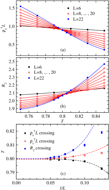
We use standard finite-size scaling Sandvik10 to extract $T_{N}$. At $T_{N}$, the stiffness constants scale with the system length as $\rho_{s}^{\alpha}\propto L^{2-d}$, where the dimensionality $d=3$. Thus, $\rho_{s}^{\alpha}L$ should be size-independent at $T_{N}$, while this quantity vanishes (diverges) for $T>T_{N}$ ($T<T_{N}$). In practice, this means that curves versus $T$ (at fixed $g$) for two different system sizes $L$ cross each other at a point which drifts (due to scaling corrections) toward $T_{N}$ with increasing $L$. The dimensionless Binder ratio also has this kind of behavior and provides us with a different $T_{N}$ estimate to check for consistency. Figs. 2(a,b) show examples of these crossing behaviors for $\rho_{s}^{x}L$ and $R_{2}$. The crossing points drift in different directions and bracket $T_{N}$. Fig. 2(c) shows the $L$ dependence of crossing points extracted from data for $(L,L+2)$ system pairs, for $R_{2}$ and two different stiffness constants. Power-law fits are used to extrapolate to infinite size. The mutual consistency of the $T_{N}$ value so obtained using different quantities gives us confidence in the accuracy of this procedure.

Figure 3: (Color online) Extrapolation of the sublattice magnetization obtained in simulations with $T=J_{1}/L$ of the double-cube Heisenberg model at different coupling ratios $g$. The error bars are much smaller than the symbols. The fitting function used for $L\to\infty$ extrapolations is $a+b/L^{2}+c/L^{3}$ (where we exclude the linear term because it comes out very close to zero in fits including it).

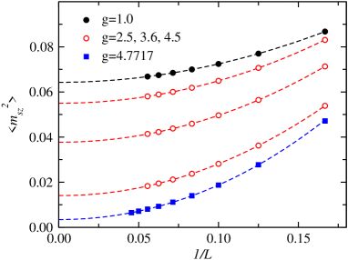
To extract the $T=0$ sublattice magnetization, we carry out simulations at temperature $T=J_{1}/L$. Note that, in a Néel phase with $T_{N}>0$, any $T(L)$ such that $T(L\to\infty)\to 0$ can be used for extrapolations to the thermodynamic limit and $T=0$. Our choice is a natural way to to scale the temperature since the lowest spin waves have energy $\propto 1/L$. We also did some calculations with $T=1/2L$ and obtained consistent extrapolated results. Examples of the $L$ dependence are shown in Fig. 3 for the double-cube model at several different coupling ratios. Taking into account rotational averaging in spin space, the final result for the sublattice magnetization is given by the $L\to\infty$ extrapolated $\langle m_{sz}^{2}\rangle$ (for which we use a polynomial fit, as shown in Fig. 3); $m_{s}=\sqrt{3\langle m_{sz}^{2}\rangle}$.

Figure 4: (Color online) The Néel temperature $T_{N}$ versus the sublattice magnetization for the three different dimerized models and with $T_{N}$ normalized in three different ways. $T_{N}$ is measured in units of (a) the inter-dimer coupling $J_{1}$, (b) the total coupling $J_{s}$ per spin, (c) the peak temperature $T^{*}$ of the susceptibility. A linear dependence obtains in all cases for small to moderate $m_{s}$, as indicate by fitted lines. Note that $m_{s}\leq 1/2$ for $S=1/2$.

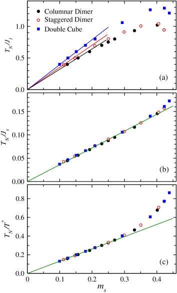
Universality of $T_{N}$ versus $m_{s}$.—Following the above procedures, we have calculated $T_{N}$ and $m_{s}$ accurately for all three dimer models at several coupling ratios $g$, from close to $g_{c}$ to deep inside the Néel phase. We graph $T_{N}$ versus $m_{s}$ in Fig. 4. $T_{N}$ is scaled by three different energy units; the inter-dimer coupling $J_{1}$ in (a), the sum of couplings $J_{s}$ connected to each spin in (b), and the temperature $T^{*}$ at which the susceptibility exhibits a peak in (c). Before discussing these normalizations of $T_{N}$ in detail, let us examine the reason for the linear behavior, $T_{N}\propto m_{s}$, seen in the QMC results for small [and in (b),(c) even quite large] $m_{s}$.

A semi-classical mean-field argument (inspired by the “renormalized classical” picture developed in two dimensions Chakravarty89 ) leading to $T_{N}\propto m_{s}$ is the following: To compute $T_{N}$ in a classical system of spins of length $S$, one replaces the coupling of a spin ${\bf S}_{0}$ to the total spin of its neighbors $\delta$, $J\sum_{\delta}{\bf S}_{\delta}$, by the thermal average $J\sum_{\delta}\langle{\bf S}_{\delta}\rangle$. In the presence of quantum fluctuations, this mean field seen by ${\bf S}_{0}$ is reduced, which is taken into account by a renormalization; $\langle{\bf S}_{\delta}\rangle\to(m_{s}/S)\langle{\bf S}_{\delta}\rangle$. The thermal fluctuations are, thus, added on top of the quantum fluctuations at $T=0$, under the assumption that the quantum effects will not change appreciably for $T>0$ (i.e., the thermal fluctuations are assumed to be solely responsible for further reducing the order). Note that ${\bf S}_{0}$ should not be renormalized here, but is computed as a thermal expectation value and should satisfy the self-consistency condition $\langle{\bf S}_{\delta}\rangle=\langle{\bf S}_{0}\rangle$. The final magnetization curve is given by $(m_{s}/S)\langle{\bf S}_{0}\rangle$. In this procedure of decoupling the classical and quantum fluctuations, one clearly effectively has $J\to(m_{s}/S)J$ and, thus, $T_{N}\propto m_{s}$.

The assumption that the quantum renormalization factor $m_{s}/S$ is $T$-independent up to $T_{N}$ can be valid only if $T_{N}$ is small. The energy scale in which to measure $T_{N}$ when stating this condition should be dictated by the spin-wave velocity, which stays non-zero at the quantum-critical point Kulik11 [i.e., not by the long-distance energy scale $\rho_{s}(T=0)$, which vanishes as $g\to g_{c}$ and is unrelated to the density of thermally excited spin waves]. A linear dependence is seen in Fig. 4 up to rather large values of $m_{s}$ (where $T_{N}\sim J_{1}$). A linear dependence was also recently found in the columnar dimer model based on high-$T$ expansions Oitmaa11 (with much larger error bars).

Returning now to the issue of how to best normalize $T_{N}$, we note that in Fig. 4(a), where the inter-dimer coupling $J_{1}$ is used, the curve for the double-cube model is significantly above the other two. This is clearly because the constant $J_{1}$ does not account for the different average couplings in the models. Using instead the sum $J_{s}$ of couplings connected to each spin, i.e., $J_{s}=5+g$ for the columnar and staggered dimers and $6+g$ for the double cube (setting $J_{1}=1$), the curves, shown in Fig. 4(b), collapse almost on top of each other. Note that also the curves for the columnar and staggered dimers are closer to each other than in Fig. 4(a), although they have the same definition of $J_{s}$. This can be the case because $J_{s}$ rescales the curves non-uniformly, since $m_{s}(g)$ and, therefore, $J_{s}(m_{s})$, is different for the two models. The linearity of $T_{N}/J_{s}$ versus $m_{s}$ is also much clearer than before and extends all the way up to $m_{s}\approx 0.3$.

Figure 5: (Color online) (a) Susceptibility versus temperature of the staggered dimer model at different coupling ratios. The system size is $L=12$, for which the peak height and location are already $L\to\infty$ converged. (b) The peak temperature versus the coupling ratio for the three different models.

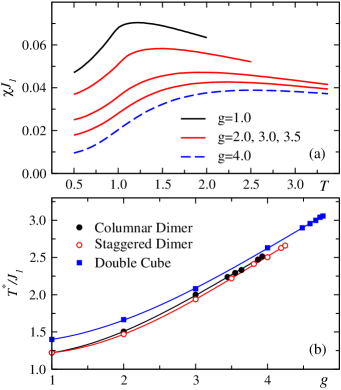
Although the data collapse is already quite good in $T_{N}/J_{s}$, we can do even better when normalizing with a physical quantity that measures the effective lattice-scale energy. One such energy scale in antiferromagnets is the temperature at which the uniform magnetic susceptibility $\chi$ exhibits a peak. This peak is due to the cross-over from the high-$T$ Curie form to the low-$T$ weakly temperature dependent form typical of antiferromagnets. The peak temperature $T^{*}$, thus, reflects the short-distance energy scale at which antiferromagnetic correlations become significant. $T^{*}$ is often used experimentally to extract the value of the exchange constant, using, e.g., the “Bonner-Fisher” curve in one dimension Eggert96 . In spatially anisotropic systems such as the dimerized models we consider here, a natural assumption is that $T^{*}$ reflects an effective average coupling. In Fig. 5(a) we show examples of the susceptibility close to its peak, and in (b) we show the dependence of $T^{*}$ on $g$ for all three models. Normalizing $T_{N}$ with $T^{*}$ leads to remarkably good data collapse, as shown in Fig. 4(c). Deviations from a common curve are barely detectable. Although we cannot prove that this function is really universal for all 3D networks of dimers, the results are very suggestive of this.

Discussion.—The universal behavior implies that the $T>0$ disordering mechanism in the 3D Néel state is completely governed by a single lattice-scale energy (which, as we have shown here, can be taken as the peak temperature $T^{*}$ of the susceptibility) and the $T=0$ sublattice magnetization $m_{s}$. The extended linear behavior seen in Figs. 4(b,c) shows that the quantum and classical fluctuations at $T<T_{N}$ are completely decoupled all the way from $g=g_{c}$ (excluding $g_{c}$ itself, where $T_{N}=0$) to quite far away from the quantum-critical point. Depending on a lattice-scale energy instead of the quantum-critical spin stiffness, the linear behavior is not fundamentally a quantum-critical effect. We have discussed the linearity and decoupling of the fluctuations in terms of a semi-classical mean-field theory, the validity of which implies that the quantum-critical regime Chubukov94 commences only above $T_{N}$. Deviations from linearity at larger $m_{s}$ show that the quantum fluctuations are affected (become $T$-dependent) here, due to the high density of excited spin waves as $T\to T_{N}$ because $T_{N}$ is high. It is remarkable that this coupling of quantum and classical fluctuations also takes place in an, apparently, universal fashion for different systems. It would be interesting to explain this more quantitatively, by deriving the full function $T_{N}$ versus $m_{s}$ analytically. Progress in the linear regime has been made recently in work parallel to ours Oitmaa11b .

From a practical point of view, the data collapse of $T_{N}/T^{*}$ versus $m_{s}$ is very useful, because all the quantities involved can be measured experimentally and do not rely on microscopic details. The universal curve can be used to test the 3D Heisenberg scenario without adjustable parameters. The universality likely applies not only to dimer netwtorks, but also to systems where the quantum fluctuations are regulated in other ways.

Acknowledgments.—We would like to thank Christian Rüegg and Oleg Sushkov for stimulating discussions. This work was supported by the NSF under Grant No. DMR-1104708.

References

- (1) S. Chakravarty, B. I. Halperin, and D. R. Nelson, Phys. Rev. B 39, 2344 (1989).
- (2) A. V. Chubukov, S. Sachdev, and J. Ye, Phys. Rev. B 49, 11919 (1994).
- (3) P. V. Shevchenko, A. W. Sandvik, and O. P. Sushkov, Phys. Rev. B 61, 3475 (2000).
- (4) S. Sachdev, Quantum Phase Transitions (Cambridge, 2001).
- (5) A. W. Sandvik, Phys. Rev. B 59, R14157 (1999).
- (6) H. G. Evertz, Adv. Phys. 52, 1 (2003).
- (7) A. W. Sandvik, AIP Conf. Proc. 1297, 135 (2010); arXiv:1101.3281 (2011).
- (8) A. W. Sandvik and D. J. Scalapino, Phys. Rev. Lett. 72, 2777 (1994); M. Matsumoto, C. Yasuda, S. Todo, and H. Takayama, Phys. Rev. B 65, 014407 (2001); L. Wang, K. S. D. Beach, and A. W. Sandvik, Phys. Rev. B 73, 014431 (2006); S. Wenzel and W. Janke, Phys. Rev. B 79, 014410 (2009).
- (9) M. Troyer, M. E. Zhitomirsky, and K. Ueda, Phys. Rev. B 55, R6117 (1997).
- (10) O. Nohadani, S. Wessel, and S. Haas, Phys. Rev. B 72, 024440 (2005).
- (11) D. X. Yao and A. W. Sandvik, Phys. Rev. B 75, 052411 (2007).
- (12) N. Cavadini et al., Phys. Rev. B 63, 172414 (2001).
- (13) Ch. Rüegg et al., Phys. Rev. Lett. 93, 257201 (2004).
- (14) Ch. Rüegg et al., Phys. Rev. Lett. 100, 205701 (2008).
- (15) M. Matsumoto, B. Normand, T. M. Rice, and M. Sigrist, Phys. Rev. B 69, 054423 (2004).
- (16) S. Sachdev, arXiv:0901.4103.
- (17) Y. Kulik and O. P. Sushkov, Phys. Rev. B 84, 134418 (2011).
- (18) J. Oitmaa and O.P. Sushkov, arXiv:1107.3617.
- (19) S. Eggert, Phys. Rev. B 53, 5116 (1996).
- (20) J. Oitmaa, Y. Kulik, and O.P. Sushkov, arXiv:1110.6478.