The Wake of a Heavy Quark in Non-Abelian Plasmas : Comparing Kinetic Theory and the AdS/CFT Correspondence

Abstract

We compute the non-equilibrium stress tensor induced by a heavy quark moving through weakly coupled QCD plasma at the speed of light and compare the result to ${\mathcal{N}}=4$ Super Yang Mills theory at strong coupling. The QCD Boltzmann equation is reformulated as a Fokker-Planck equation in a leading log approximation which is used to compute the induced stress. The transition from non-equilibrium at short distances to equilibrium at large distances is analyzed with first and second order hydrodynamics.

Even after accounting for the obvious differences in shear lengths, the strongly coupled theory is significantly better described by hydrodynamics at sub-asymptotic distances. We argue that this difference between the kinetic and AdS/CFT theories is related to the second order hydrodynamic coefficient $\tau_{\pi}$. $\tau_{\pi}$ is numerically large in units of the shear length for theories based on the Boltzmann equation.

I Introduction

The goal of the relativistic heavy ion programs at RHIC and the LHC is to create and study the properties of the Quark Gluon Plasma (QGP). Since the real time dynamics can not be directly probed with the Lattice QCD, the transport properties of QGP are of particular interest. There is a consensus that the experimental results on collective flow imply that the shear viscosity to entropy ratio of the Quark Gluon Plasma is remarkably small *[Forareviewofthedegreeofconsensusandreferencessee:]Teaney:2009qa

$$\frac{\eta}{s}\sim\frac{1\leftrightarrow 5}{4\pi}\,.$$ (1)

Although it is difficult to reconcile this experimental ratio with a quasi-particle picture of the plasma, the success of resummed perturbation theory at describing lattice data on the pressure at somewhat higher temperatures suggests that a quasi-particle picture might provide a qualitative guide to the plasma dynamics and form a basis for further approximation schemes Blaizot et al. (2003); Andersen et al. (2011a, b).

However, in ${\mathcal{N}}=4$ Super Yang Mills (SYM) theory at strong coupling (and large $N_{c}$) gauge-gravity duality can be used to compute the shear to entropy ratio exactly Policastro et al. (2001); Kovtun et al. (2005),

$$\frac{\eta}{s}=\frac{1}{4\pi}\,.$$ (2)

The tantalizing similarity between the experimental ratio and this celebrated theoretical result hints that a strong coupling limit (without quasi-particles) might provide a better starting point for understanding the plasma dynamics. At the very least, the strongly coupled ${\mathcal{N}}=4$ theory is an analytically tractable limit that provides a useful foil to perturbative calculations based on a quasi-particle description.

The goal of this work is to compare the steady state response of non-abelian plasma at weak and strong coupling to an infinitely heavy quark probe moving at the speed of light. This is the simplest setup where the plasma response to an energetic probe can be analyzed in detail Stoecker (2005); Casalderrey-Solana et al. (2005); Gubser et al. (2008); Yarom (2007); Chesler and Yaffe (2007, 2008); Neufeld (2008). At long distances, the non-equilibrium disturbance produced by the heavy quark probe thermalizes and forms a Mach cone and diffusion wake. The original motivation for investigating the Mach cone was the observation of an unusual structure in measured two particle correlations Adare et al. (2008); Abelev et al. (2009). Today, after the analysis of Alver and Roland Alver and Roland (2010) and others Takahashi et al. (2009); Sorensen (2010); Lin et al. (2005); Ma et al. (2006), these unusual correlations are understood as the hydrodynamic response to fluctuations in the initial geometry and not as the medium response to an energetic probe. (The Mach cone picture also dramatically fails to explain current measurements in several ways – see for example Ref. Chaudhuri and Heinz (2006) and the conclusions of Ref. Casalderrey-Solana et al. (2006).) The goal of this manuscript is not to explain current measurements, but rather to examine the differences between weak and strong coupling, and to study the approach to hydrodynamics in both cases. Although the current paper has no immediate phenomenological goals, the medium response to energetic partons is currently being studied by all the experimental collaborations in various ways [SeeforexampletherecentanalysisbytheCMScollaboration:]Chatrchyan:2011sx. Thus, this calculation, which analyzes the “jet” medium interaction precisely and determines a source for hydrodynamics through second order in the gradient expansion, may be useful for phenomenology in further studies.

In the strongly coupled theory the stress tensor induced by a finite velocity heavy quark was computed using the AdS/CFT correspondence Chesler and Yaffe (2007); Gubser et al. (2008). The approach to hydrodynamics was analyzed as well as the short distance behavior Chesler and Yaffe (2008); Yarom (2007); Gubser and Pufu (2008). In particular we will largely follow (and to a certain extent extend) the hydrodynamic analysis of Ref. Chesler and Yaffe (2008) to determine a hydrodynamic source through second order in the gradient expansion for the kinetic and strongly coupled theories. In the AdS/CFT calculation the lightlike $v\rightarrow c$ limit was not analyzed due to various technical complications. (Here and below $v$ is the velocity of the heavy quark.) As discussed in Section II.2, it is possible to set $v=c$ throughout the calculation by choosing a different set of gauge invariants.

At weak coupling the hydrodynamic source has not been computed. Nevertheless the appropriate source for kinetic theory was determined in Ref. Neufeld (2008), and several estimates have been given for how this kinetic source is transformed through the relaxation process to hydrodynamics Neufeld (2009). We have simplified the source for kinetic theory considerably and determined the plasma response at large distances by solving the linearized kinetic theory. After comparing the hydrodynamic solution at large distances to the full (leading-log) kinetic theory results, the appropriate source at each order in the hydrodynamic expansion can be computed. This part of the calculation employs a computer code developed by us to determine spectral functions at finite $\omega$ and $k$ Hong and Teaney (2010). As a by-product of these spectral functions we determined the hydrodynamic transport coefficients that appear through second order in the gradient expansion in a leading log approximation. These parameters will be needed below to precisely determine the hydrodynamic source through second order.

This work is limited to the analysis of the kinetics for a single heavy quark moving from past infinity. It would be quite interesting to follow the evolution of a parton shower initiated at time $t=0$ and the subsequent hydrodynamic response at late times. Although this transition has not been worked out, several of the most important ingredients have already been clarified Neufeld and Muller (2009); Neufeld and Vitev (2011); Arnold et al. (2010). We hope to address the thermalization of full parton showers in future work.

II Preliminaries

We consider an infinitely heavy quark with $v\simeq 1$ moving through a stationary high temperature plasma from past infinity. We will calculate the medium response in two model theories – pure glue QCD at asymptotically weak coupling and ${\mathcal{N}}=4$ SYM at asymptotically strong coupling. Both theories are conformal in this limit and therefore the background stress tensor takes the characteristic form

$$T^{\mu\nu}_{o}={\rm diag}(e,{\mathcal{P}},{\mathcal{P}},{\mathcal{P}})\,,\qquad\mbox{with}\qquad e=3{\mathcal{P}}.$$ (3)

The heavy quark moves in the $\hat{{\bm{z}}}$ direction and imparts energy and momentum to the plasma, which ultimately induces a non-equilibrium response, $\delta T^{\mu\nu}$. The non-equilibrium stress tensor $\delta T^{00}$ and $\delta T^{0z}$ are functions of cylindrical and comoving coordinates $x_{T}$ and $x_{L}$ where

$$x_{T}=\sqrt{x^{2}+y^{2}}\,,\qquad\varphi_{r}={\rm atan2}(y,x)\,,\qquad\mbox{and}\qquad x_{L}=z-vt\,.$$ (4)

Rotational invariance around the $z$ axis determines $(T^{0x},T^{0y})$ in terms of $T^{0x_{T}}$

$$T^{0x}(t,{\bm{x}})= T^{0x_{T}}(x_{L},x_{T})\cos\varphi_{r}\,,$$ (5)

$$T^{0y}(t,{\bm{x}})= T^{0x_{T}}(x_{L},x_{T})\sin\varphi_{r}\,.$$ (6)

II.1 Kinetic Theory with a Heavy Quark Probe

At weak coupling kinetic theory determines the response of the plasma to the heavy quark probe. To determine this response we linearize the Boltzmann equation for $f(t,{\bm{x}},{\bm{p}})=n_{p}+\delta f(t,{\bm{x}},{\bm{p}})$ with $n_{p}=1/(e^{p/T_{o}}-1)$ and will restrict the calculation to pure glue QCD in a leading log-approximation for simplicity. The Boltzmann equation in this limit reads

$$\left(\partial_{t}+{\bm{v}}_{p}\cdot\partial_{{\bm{x}}}\right)\delta f(t,{\bm{x}},{\bm{p}})=C[f,{\bm{p}}]+S(t,{\bm{x}},{\bm{p}})\,,$$ (7)

where ${\bm{v}}_{\bm{p}}=\hat{{\bm{p}}}$ and $S(t,{\bm{x}},{\bm{p}})$ is the (to be discussed) source of non-equilibrium gluons produced by the heavy quark moving through the plasma. In a leading $\log(T/m_{D})$ approximation, the linearized collision integral simplifies to a momentum diffusion equation supplemented by gain terms Hong and Teaney (2010)

$$C[f,{\bm{p}}] = T\mu_{A}\frac{\partial}{\partial{\bm{p}}^{i}}\left(n_{p}(1+n_{p})\frac{\partial}{\partial{\bm{p}}^{i}}\left[\frac{\delta f}{n_{p}(1+n_{p})}\right]\right)+\mbox{gain terms}\,,$$

$$\mu_{A} \equiv \frac{g^{2}C_{A}m_{D}^{2}}{8\pi}\log\left(\frac{T}{m_{D}}\right)\,.$$ (8)

Here the Debye mass for a pure glue theory is

$$m_{D}^{2}=2g^{2}T_{A}\int\frac{{\rm d}^{3}{\bm{p}}}{(2\pi)^{3}}\frac{n_{p}(1+n_{p})}{T}=\frac{g^{2}T^{2}}{3}N_{c}\,,$$ (9)

where $T_{A}=N_{c}$ is the trace normalization of the adjoint representation. The diffusion equation should be solved with absorptive boundary conditions at $p=0$ so the number of particles is not conserved during the evolution Arnold et al. (2006). Thus the microscopic theory encoded by this diffusion equation is conformal, and the only conserved quantities are energy and momentum.

The gain terms are responsible for energy and momentum conservation. Specifically, the energy and momentum that is transferred (per time, per degree of freedom, per volume) to the non-equilibrium excess $\delta f$ by equilibrium bath is

$$\frac{{\rm d}E}{{\rm d}t}\equiv -T\mu_{A}\int\frac{{\rm d}^{3}{\bm{p}}}{(2\pi)^{3}}\,n_{p}(1+n_{p})\,\hat{\bm{p}}\cdot\frac{\partial}{\partial{\bm{p}}}\left[\frac{\delta f}{n_{p}(1+n_{p})}\right]\,,$$ (10)

$$\frac{{\rm d}{\bm{P}}}{{\rm d}t}\equiv -T\mu_{A}\int\frac{{\rm d}^{3}{\bm{p}}}{(2\pi)^{3}}\,n_{p}(1+n_{p})\,\frac{\partial}{\partial{\bm{p}}}\left[\frac{\delta f}{n_{p}(1+n_{p})}\right]\,,$$ (11)

as can easily be found by integrating both sides of Eq. (7) without the source. This energy and momentum transfer by the bath drives additional particles away from equilibrium and ultimately fixes the structure of the gain terms:

$$\mbox{gain terms}=\frac{1}{\xi_{B}}\left[\frac{1}{p^{2}}\frac{\partial}{\partial p}p^{2}n_{p}(1+n_{p})\right]\frac{{\rm d}E}{{\rm d}t}+\frac{1}{\xi_{B}}\left[\frac{\partial}{\partial{\bm{p}}}n_{p}(1+n_{p})\right]\cdot\frac{{\rm d}{\bm{P}}}{{\rm d}t}\;,$$ (12)

where for subsequent use we have defined

$$\xi_{B}\equiv\int\frac{{\rm d}^{3}{\bm{p}}}{(2\pi)^{3}}n_{p}(1+n_{p})=\frac{T^{3}}{6}\,.$$ (13)

With the gain terms it is easy to verify that energy and momentum are conserved. Previously we analyzed the linear response of this system of equations and determined the hydrodynamic plasma parameters in terms of $\mu_{A}$ Hong and Teaney (2010)

$$\frac{\eta}{e+P}= 0.4613\,\frac{T}{\mu_{A}}\,,$$ (14)

$$\frac{\tau_{\pi}}{\eta/sT}= 6.32\,.$$ (15)

Since the microscopic dynamics is conformal, linearized, and only conserves energy and momentum (and not particle number), $\tau_{\pi}$ is the only second order hydrodynamic coefficient that appears to this order. If there are additional conserved quantities and the dynamics is not conformal then there are a multitude of coefficients that appear at second order – see for example Romatschke (2010); Betz et al. (2011). Further it must be emphasized that these second order transport coefficients are insufficient to describe the decay of initial transients (non-hydrodynamic modes) Betz et al. (2011).

The shear viscosity naturally agrees with prior results Baym et al. (1990); Arnold et al. (2000). The fact that $\tau_{\pi}$ is somewhat large $\sim 6$ compared to the viscous length is a generic result of kinetic theory Baier et al. (2008); York and Moore (2009). Finally, we note that $\mu_{A}$ records the transverse momentum broadening of a bath particle due to the soft scatterings, and is related to the soft part of jet-quenching $\hat{q}$ parameter in a leading $T/m_{D}$ approximation Arnold and Xiao (2008), $\hat{q}_{\rm soft}/2=2T\mu_{A}$. Thus, the leading-log limit provides a concrete relation between $\eta/s$ and $\hat{q}$.

We now analyze how a heavy quark disturbs this system in the same leading log approximation scheme. The leading log energy loss of the heavy quark was computed long ago by Braaten and Thoma Braaten and Thoma (1991a, b), with the result that the momentum transferred to the medium per time (i.e. minus the drag-force) is

$$\frac{{\rm d}p^{\mu}}{{\rm d}t}=\left(\frac{{\rm d}E}{{\rm d}t},\frac{{\rm d}{\bm{p}}}{{\rm d}t}\right)=\mu_{F}(v)\,\Big{(}v^{2},{\bm{v}}\Big{)}\,,$$ (16)

where $\mu_{F}(v)$ is the drag coefficient in a leading log approximation

$$\mu_{F}(v)= \frac{g^{2}C_{F}m_{D}^{2}}{8\pi}\log\left(\frac{T}{m_{D}}\right)\left(\frac{1}{v^{2}}-\frac{1-v^{2}}{2v^{3}}\log\left(\frac{1+v}{1-v}\right)\right)\,,$$ (17)

$$\Rightarrow \frac{g^{2}C_{F}m_{D}^{2}}{8\pi}\log\left(\frac{T}{m_{D}}\right)\,.$$ (18)

In the last line we have taken the $v\rightarrow 1$ limit of relevance to this work. As discussed more completely below, we have implicitly taken the coupling to zero before taking this limit so that radiative energy loss can be neglected.

The drag force arises as equilibrium gluons from the bath scatter off the heavy quark probe and are driven out of equilibrium by the scattering process. This scattering produces a source of non-equilibrium gluons located at the position of the quark,

$$S(t,{\bm{x}},{\bm{p}})=S({\bm{p}})\,\delta^{3}({\bm{x}}-{\bm{v}}t)\,.$$

Appendix A analyzes this scattering process ($g+Q\rightarrow g+Q$) and determines the appropriate momentum space source, $S({\bm{p}})$. In the limit $v=1$ the source has a simple form involving only two spherical harmonics

$$S({\bm{p}}) = \mu_{F}\,\frac{n_{p}(1+n_{p})}{2d_{A}\xi_{B}}\left[-\frac{2}{p}+\frac{(1+2n_{p})}{T}+\frac{(1+2n_{p})}{T}\,\hat{{\bm{p}}}\cdot{\hat{\bm{v}}}\right],\qquad\mbox{for $v=1$ \, . }$$ (19)

With this source it is straightforward to integrate $2d_{A}\int\frac{{\rm d}^{3}{\bm{p}}}{(2\pi)^{3}}p^{\mu}$ over Eq. (7) and to verify that the stress tensor satisfies

$$\partial_{\mu}\,\delta T^{\mu\nu}=\frac{{\rm d}p^{\nu}}{{\rm d}t}\,\delta^{3}({\bm{x}}-{\bm{v}}t)\,.$$ (20)

Our strategy to determine the energy-momentum tensor is the following. We take the Fourier transform with respect to ${\bm{x}}$ of the kinetic equation in Eq. (7)

$$(-i\omega+i{\bm{v}}_{p}\cdot{\bm{k}})\delta f(\omega,{\bm{k}},{\bm{p}})=C[\delta f,{\bm{p}}]+2\pi S({\bm{p}})\delta(\omega-{\bm{v}}\cdot{\bm{k}})\,,$$ (21)

and solve the Boltzmann equation in Fourier space. The technology to do this is based on simple matrix inversion as was documented in Ref. Hong and Teaney (2010). Then we calculate the stress energy tensor in Fourier space using kinetic theory. By Fourier transforming the stress tensor back to coordinate space, we can determine the energy and momentum density distributions. Additional details about this procedure are given in Appendix B.

II.2 AdS/CFT with a heavy quark probe

To describe the response of the ${\mathcal{N}}=4$ plasma to a heavy quark probe we will follow the notations and conventions of Refs. Chesler and Yaffe (2007); Athanasiou et al. (2010) which should be referred to for all details. Briefly, a heavy quark is described in ${\rm AdS}_{5}$ with a trailing string. The energy and momentum gained by the medium as the heavy quark traverses the plasma is again parameterized with the drag coefficient $\mu_{F}(v)$

$$\frac{{\rm d}p^{\mu}}{{\rm d}t}=\left(\frac{{\rm d}E}{{\rm d}t},\frac{{\rm d}{\bm{p}}}{{\rm d}t}\right)=\mu_{F}(v)\Big{(}v^{2},{\bm{v}}\Big{)}\,.$$ (22)

This coefficient is found by determining the energy and momentum flowing down the string into the black hole Herzog et al. (2006); [][.Thisworkwaslimitedtothenon-relativisticlimit.]CasalderreySolana:2006rq; Gubser (2006)

$$\mu_{F}(v)=\frac{\pi}{2}\frac{\sqrt{\lambda}T^{2}}{\sqrt{1-v^{2}}}\,.$$ (23)

As in the weakly coupled case, the stress tensor in the strongly coupled ${\mathcal{N}}=4$ theory satisfies Eq. (20) with the energy-momentum transfer rates given by the corresponding strongly coupled formulas. The deposited energy and momentum leads ultimately to a hydrodynamic response in the strongly coupled theory. The linearized hydrodynamic parameters through second order are Policastro et al. (2001); Baier et al. (2008); Bhattacharyya et al. (2008)

$$\frac{\eta}{e+P}= \frac{1}{4\pi T}\,,$$ (24)

$$\frac{\tau_{\pi}}{\eta/(e+P)}= 4-2\log(2)\simeq 2.61\,.$$ (25)

According to AdS/CFT duality Maldacena (1998), strongly coupled SYM plasma is dual to the $5d$ AdS-Schwarzschild geometry, which has the metric

$$ds^{2}=\frac{L^{2}}{u^{2}}\left[-f(u)dt^{2}+d{\bm{x}}^{2}+\frac{du^{2}}{f(u)}\right]\,.$$ (26)

Here $u$ is the radial coordinate of the AdS geometry with $u=0$ corresponding to the boundary, $L$ is the AdS curvature radius, $f(u)=1-u^{4}/u_{h}^{4}$ with $u_{h}=1/\pi T$, and $T$ is the (Hawking) temperature of the plasma and dual geometry.

The addition of an infinitely massive fundamental quark to the SYM plasma is dual to the addition of a string to the AdS Schwarzschild geometry, with the string ending at $u=0$ Karch and Katz (2003). The presence of the string perturbs the $5d$ geometry according to Einstein’s equations and the near boundary behavior of the metric perturbation encodes the changes in the SYM stress tensor due to the presence of the quark de Haro et al. (2001).

In the large $N$ limit the $5d$ gravitational constant $\kappa_{5}^{2}\sim 1/N^{2}$ is small. Consequently the back-reaction of the string on the geometry can be treated perturbatively by solving the string equations in the background metric and subsequently computing the metric perturbations sourced by the string. Solving the string equations of motion leads to the well known trailing string profile Herzog et al. (2006); Gubser (2006)

$$\bm{x}_{\rm string}(t,u)=\bm{v}\left[t+\frac{u_{h}}{2}\left(\tan^{-1}\frac{u}{u_{h}}+\frac{1}{2}\log\frac{u_{h}-u}{u_{h}+u}\right)\right].$$ (27)

This string profile describes a quark moving at constant velocity $\bm{v}$ and has the $5d$ stress tensor

$$t_{0i} =-v_{i}F, t_{ij} =v_{i}v_{j}F, t_{00} =\frac{u^{4}v^{2}+uh^{4}f}{uh^{4}}F,$$ (28a)

$$t_{05} =-\frac{u^{2}v^{2}}{u_{h}^{2}f}F, t_{i5} =\frac{u^{2}v_{i}}{u_{h}^{2}f}F, t_{55} =\frac{v^{2}-f}{f^{2}}F,$$ (28b)

where

$$F=\frac{u\sqrt{\lambda}}{2\pi L^{3}\sqrt{1-v^{2}}}\delta^{3}(\bm{x}-\bm{x}_{\rm string}),$$ (29)

and $\lambda$ is the ’t Hooft coupling.

The five dimensional stress tensor of the string perturbs the background geometry. The information contained in the linear metric perturbation sourced by the trailing string can be conveniently packaged into fields which are invariant under infinitesimal diffeomorphisms Athanasiou et al. (2010); Chesler and Yaffe (2008). Defining

$$G_{MN}\equiv G_{MN}^{(0)}+\frac{L^{2}}{u^{2}}H_{MN}\,,$$ (30)

where $G_{MN}^{(0)}$ is the background metric (26) and $H_{MN}$ is the perturbation, and introducing a space-time Fourier transform

$$H_{MN}(t,\bm{x},u)=\int\frac{{\rm d}\omega}{2\pi}\frac{{\rm d}^{3}{\bm{q}}}{(2\pi)^{3}}H_{MN}(\omega,\bm{q},u)e^{-i\omega t+i\bm{q}\cdot\bm{x}},$$ (31)

we find two convenient diffeomorphism invariant fields Athanasiou et al. (2010); Chesler and Yaffe (2008)

$$Z_{0}\equiv \frac{4f}{\omega}q^{i}H^{\prime}_{0i}-\frac{4f^{\prime}}{\omega}q^{i}H_{0i}-\frac{2f^{\prime}}{q^{2}}q^{i}q^{j}H_{ij}+4ifq^{i}H_{i5}$$

$$\qquad\qquad\qquad\qquad-\frac{(2uq^{2}{-}f^{\prime})}{q^{2}}\left(q^{2}\delta^{ij}{-}q^{i}q^{j}\right)H_{ij}+\frac{4q^{2}f}{i\omega}H_{05}-\frac{8\kappa_{5}^{2}f}{i\omega}t_{05}\,,$$ (32)

$$\bm{Z}_{1}\equiv \left(H^{\prime}_{0i}-i\omega\,H_{i5}\right)\hat{\epsilon}^{i}_{a}\hat{\bm{\epsilon}}_{a}\,.$$ (33)

Here sums over repeated indices are implied with $i,j$ running from 1 to 3 and $a$ running from 1 to 2, ^′ denotes differentiation with respect to $u$ and

$$\hat{\bm{\epsilon}}_{1}=\frac{q}{q_{\perp}}\,\hat{\bm{q}}\times(\hat{\bm{v}}\times\hat{\bm{q}})\,,\quad\hat{\bm{\epsilon}}_{2}=\frac{q}{q_{\perp}}\,\hat{\bm{v}}\times\hat{\bm{q}}\,.$$ (34)

The field $Z_{0}$ transforms as a scalar under rotations and the field $\bm{Z}_{1}$ transforms as a vector under rotations.

The equations of motion for $Z_{0}$ and $\bm{Z}_{1}$ are straightforward but tedious to derive from the linearized Einstein equations. They read

$$Z_{0}^{\prime\prime}+A_{0}Z_{0}^{\prime}+B_{0}Z_{0}=\kappa_{5}^{2}S_{0}\,,$$ (35)

where

$$A_{0} \equiv-\frac{24+4q^{2}u^{2}+6f+q^{2}u^{2}f-30f^{2}}{uf\left(u^{2}q^{2}+6-6f\right)}\,,$$ (36)

$$B_{0} \equiv\frac{\omega^{2}}{f^{2}}+\frac{q^{2}u^{2}(14{-}5f{-}q^{2}u^{2})+18(4{-}f{-}3f^{2})}{u^{2}f\left(q^{2}u^{2}+6-6f\right)}\,,\ \ \ \ \ \ \ \$$ (37)

$$S_{0} \equiv\frac{8}{f}t^{\prime}_{00}+\frac{4\left(q^{2}u^{2}{+}6{-}6f\right)}{3uq^{2}f}(q^{2}\delta^{ij}{-}3q^{i}q^{j})t_{ij}$$ (38)

$$\qquad+\frac{8i\omega}{f}t_{05}+\frac{8u\left[q^{2}\left(q^{2}u^{2}{+}6\right)-f\left(12q^{2}{-}9f^{\prime\prime}\right)\right]}{3f^{2}\left(q^{2}u^{2}-6f+6\right)}t_{00}-\frac{8q^{2}u}{3}t_{55}-8iq^{i}t_{i5}\,.$$

and

$$\bm{Z}^{\prime\prime}_{1}+A_{1}\,\bm{Z}^{\prime}_{1}+B_{1}\,\bm{Z}_{1}=\kappa_{5}^{2}\bm{S}_{1}\,,$$ (39)

where

$$A_{1} \equiv\frac{uf^{\prime}-3f}{uf}\,,$$ (40)

$$B_{1} \equiv\frac{3f^{2}-u\left(uq^{2}+3f^{\prime}\right)f+u^{2}\omega^{2}}{u^{2}f^{2}}\,,$$ (41)

$$\bm{S}_{1} \equiv\frac{2}{f}\,\Big{[}t^{\prime}_{0i}+i\omega\,t_{i5}\Big{]}\hat{\epsilon}^{i}_{a}\hat{\bm{\epsilon}}_{a}.$$ (42)

We note that since the string stress tensor (28) only depends on time through the combination $\bm{x}-\bm{v}t$, when Fourier transformed, the string stress tensor is proportional to $2\pi\delta(\omega-\bm{v}\cdot\bm{q})$. Consequently the fields $Z_{s}$ are also proportional to $2\pi\delta(\omega-\bm{v}\cdot\bm{q})$. Moreover, because the string stress tensor (28) is proportional to $1/\sqrt{1-v^{2}}$ and Eqs. (35) and (39) are linear, we define $Z_{s}=\tilde{Z}_{s}/\sqrt{1-v^{2}}$ and solve for $\tilde{Z}_{s}$ in the $v\to 1$ limit.

Under the assumption that the boundary geometry is flat, near the boundary the fields $Z_{s}$ have the asymptotic expansions

$$\tilde{Z}_{s}(u)=\tilde{Z}_{s}^{(2)}u^{2}+\tilde{Z}_{s}^{(3)}u^{3}+\tilde{Z}_{s}^{(4)}u^{4}+\dots.$$ (43)

The cubic expansion coefficients $\tilde{Z}_{s}^{(3)}$ determine the SYM energy density $\delta T^{00}$ and the SYM energy flux $\delta T^{0i}$ via Athanasiou et al. (2010); Chesler and Yaffe (2008)

$$\delta T^{00}= -\frac{L^{3}}{8\kappa_{5}^{2}}\frac{1}{\sqrt{1-v^{2}}}\tilde{Z}^{(3)}_{0}\,,$$ (44)

$$\delta T^{0i}= -\frac{L^{3}}{2\kappa_{5}^{2}}\frac{1}{\sqrt{1-v^{2}}}\left[({\tilde{Z}_{1}^{(3)}})^{i}+\frac{\omega q^{i}}{4q^{2}}(\tilde{Z}^{(3)}_{0})^{i}\right]-\frac{iq^{i}\mu_{F}(v)v^{2}}{q^{2}}.$$ (45)

For a given momentum $\bm{q}$, to determine the SYM energy density and energy flux we solve Eqs. (35) and (39) using pseudospectral methods. At the boundary at $u=0$ we impose the boundary condition that the fields have asymptotics of the form given in the series expansions (43), which is tantamount to demanding that the boundary geometry is flat. At the horizon at $u=u_{h}$ we impose the boundary condition of infalling waves. This is tantamount to demanding that $\tilde{Z}_{s}\sim(u-u_{h})^{-i\omega u_{h}/4}$ near the horizon. With the $\tilde{Z}_{s}$ known, we can then extract the expansion coefficients $\tilde{Z}_{s}^{(3)}$ and construct the SYM energy density and energy flux from Eq. (44) and Eq. (45) .

III Comparing AdS/CFT and Kinetic Theory

Using the formalism outlined in the previous section we compute the energy density and Poynting vector induced by the heavy quark in both kinetic theory and the AdS/CFT correspondence. To compare the AdS/CFT and the kinetic theory results we have measured all length-scales in units of the shear length

$${L_{o}}\equiv\frac{\textstyle{\frac{4}{3}}\eta c}{(e+{\mathcal{P}})c_{s}^{2}}$$ (46)

where $c_{s}^{2}$ is the squared sound speed and in practice the speed of light is set to unity. ${L_{o}}$ is proportional to the mean free path in kinetic theory and equal to $1/\pi T$ for the ${\mathcal{N}}=4$ theory. At large distances, where ideal hydrodynamics is applicable, the amplitude of the disturbance is proportional to the strength of the energy loss. Thus, we divide the response by the corresponding drag coefficient $\mu_{F}(v)$ for each theory, Eq. (17) and Eq. (23). With these rescalings the two theories produce the same (rescaled) stress tensor at asymptotically large distances, but differ in their approach to the ideal hydrodynamic limit as we will analyze in Section IV. Fig. 1 and Fig. 2 compare the non-equilibrium stress in the two cases. A complete discussion is reserved for the summary in Section V.

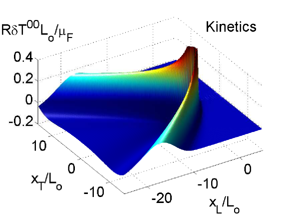
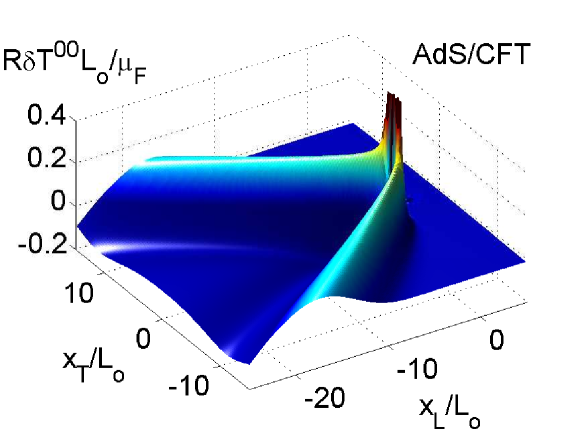
Figure 1: The energy density (in scaled units) times $R=\sqrt{x_{T}^{2}+x_{L}^{2}}$ that is induced by a heavy quark probe in (a) weakly coupled QCD and (b) strongly coupled ${\mathcal{N}}=4$ SYM. Here ${L_{o}}$ is the shear length and the $\mu_{F}(v)$ is the drag coefficient for each case (see text).

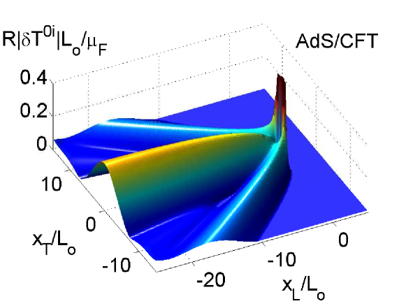
Figure 2: The magnitude of the Poynting vector $|T^{0i}|$ (in scaled units) times $R=\sqrt{x_{T}^{2}+x_{L}^{2}}$ that is induced by a heavy quark probe in (a) weakly coupled QCD and (b) strongly coupled ${\mathcal{N}}=4$ SYM. Here ${L_{o}}$ is the shear length and the $\mu_{F}(v)$ is the drag coefficient for each case (see text).

In order to compare the stress tensor quantitatively we plot the energy density in concentric circles of radius $R$ around the head of the quark. Specifically, we define

$$\frac{\rm{d}E_{R}}{\rm{d}\theta_{R}}=2\pi R^{2}\sin\theta_{R}\,\delta T^{00}(\mathbf{R})\,,$$ (47)

where $\mathbf{R}=x_{T}\hat{{\bm{x}}}_{T}+x_{L}\hat{{\bm{z}}}$ and the polar angle is measured from the direction of the quark $\hat{{\bm{z}}}$:

$$\begin{minipage}[c]{60.70653pt} \includegraphics[width=433.62pt]{angles.pdf} \end{minipage}\,.$$ (48)

Similarly, the angular distribution of the energy flux is given by

$$\frac{\rm{d}S_{R}}{\rm{d}\theta_{R}} = 2\pi R^{2}\sin\theta_{R}\,\hat{R}^{i}\delta T^{0i}(\mathbf{R})\,,$$ (49)

$$= 2\pi R^{2}\sin\theta_{R}\left[\cos\theta_{R}\,\delta T^{0z}(\mathbf{R})+\sin\theta_{R}\,\delta T^{0x}(\mathbf{R})\right]\,.$$

Numerical results for the angular distributions of the energy density and flux at several scaled distances $\mathfrak{R}\equiv R/{L_{o}}$ are shown in Fig. 3.

There is a dramatic change in the AdS/CFT curves between $\mathfrak{R}=1$ and $\mathfrak{R}=5$, indicating a transition from hydrodynamic behavior to quantum dynamics at distances of order $\sim 1/\pi T$. Since this quantum dynamics lies beyond the semi-classical Boltzmann approximation, no transition is seen in the kinetic theory curves. It would be interesting to calculate the stress tensor in this region perturbatively to better understand the differences between the two theories for $R\sim 1/\pi T$.

Let us pause to discuss the limitations of both calculations. The point of the current work is to compare the approach to hydrodynamics at infinitely weak and infinitely strong coupling. In both cases the coupling is taken to zero or infinity before the limit, $v\rightarrow 1$. As we now discuss, this limits the lengths scales that can be meaningfully studied in both theories.

In the kinetic theory calculation the resulting stress tensor is valid for distances, $R\gg 1/(g^{2}T\log g^{-1})$. For distances shorter than $1/(g^{2}T\log g^{-1})$ the collisionless non-abelian Vlasov equations should be used to describe the medium response at weak coupling Elze and Heinz (1989); Blaizot and Iancu (2002). However, for distances longer than $1/(g^{2}T\log g^{-1})$ the effect of the plasma dynamics is incorporated into the polarization tensor of the soft collisional integrals between the heavy quark and the particles that make up the bath. For example, the drag coefficient computed by Braaten and Thoma includes an HTL propagator in the t-channel exchange that includes the plasma physics of the polarization tensor Bellac (1996). We have limited the evaluation of this polarization tensor to a leading log approximation.

Further, the weakly coupled calculation is limited to modest $\gamma$. We have implicitly taken the coupling constant to zero before taking $v\rightarrow 1$ so that the radiative energy loss of the heavy quark can be neglected. For a small but finite coupling constant radiative energy loss is suppressed when the Lorentz gamma factor of the heavy quark is not too large Moore and Teaney (2005), $\gamma\mbox{~{}{\raisebox{1.72218pt}{$<$}} {\raisebox{-2.58334pt}{$\sim$}}~{}}\frac{m_{D}}{T\alpha_{s}}\sim 1/g$.

Similarly, the AdS/CFT calculation is limited to comparatively large distances $x_{L},x_{T}\gg 1/\sqrt{\gamma}\pi T$. In Section II.2 we introduced a new set of helicity variables so that the medium response on distances much greater than $1/\sqrt{\gamma}\pi T$ can be determined in the limit when $v=1$. For distances much less than $1/\sqrt{\gamma}\pi T$ the structure of stress tensor has been analyzed in detail Yarom (2007); Gubser and Pufu (2008); Noronha et al. (2009). The medium response is characterized by a transverse length scale of $1/\sqrt{\gamma}\pi T$, and a corresponding longitudinal scale of $1/\gamma^{3/2}\pi T$, where $\gamma$ is the Lorentz factor of the heavy quark. In Fig. 3 we are investigating distances of order $x_{L},x_{T}\sim 1/\pi T$ and the physics associated with these very short scales is not visible. Although the importance of the $1/\sqrt{\gamma}\pi T$ scale was understood in the context of momentum fluctuations Gubser (2008); Casalderrey-Solana and Teaney (2007); Dominguez et al. (2008), it is instructive to see these scales reappear in the asymptotic expansion for the induced stress tensor at short distances Yarom (2007); Gubser and Pufu (2008). Rewriting Eq. (137) of Ref. Gubser and Pufu (2008) in terms of $\gamma$, and expanding for $\gamma$ large with $\tilde{x}_{L}\equiv\gamma x_{L}$ of order $x_{T}$, we have

$$\frac{1}{\sqrt{\lambda}}\left\langle\delta T^{00}(x_{L},x_{T})\right\rangle=\frac{\gamma^{2}x_{T}^{2}}{6\pi^{2}\left(\tilde{x}_{L}^{2}+x_{T}^{2}\right)^{3}}+\frac{T^{2}\gamma^{3}}{24}\frac{\left(2\tilde{x}_{L}^{3}+\tilde{x}_{L}x_{T}^{2}\right)}{\left(\tilde{x}_{L}^{2}+x_{T}^{2}\right)^{5/2}}+\ldots\,.$$ (50)

The first term is the leading term at short distances and is independent of temperature. The second term (which captures the first finite temperature correction) is subleading in inverse powers of distance, but enhanced by a power of $\gamma$. Comparing the magnitude of these terms we see that the first term will dominate provided

$$\sqrt{(\gamma x_{L})^{2}+x_{T}^{2}}\mbox{~{}{\raisebox{1.72218pt}{$<$}} {\raisebox{-2.58334pt}{$\sim$}}~{}}\frac{1}{\sqrt{\gamma}\pi T}\,.$$ (51)

This constraint limits the validity (and utility) of the short distance expansion to rather short distances.

In summary we are examining two extreme limits – infinitely weak and infinitely strong coupling. The disadvantage of this approach is that some of the marked differences at short distances between the Vlasov response of weakly coupled QCD and the AdS/CFT response are not visible (see especially Betz et al. (2009)). The advantage of this approach is that the onset of hydrodynamics can be clearly compared. We will analyze the hydrodynamic limit in the next section.

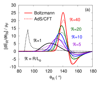
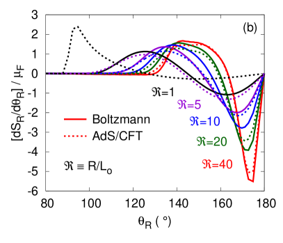
Figure 3: The angular distribution of (a) the energy density $[\rm{d}E_{R}/\rm{d}\theta_{R}]/\mu_{F}$ and (b) the energy flux $[\rm{d}S_{R}/\rm{d}\theta_{R}]/\mu_{F}$ at distances $\mathfrak{R}=1,\,5,\,10,\,20,\,\mbox{and}\,40$ for the kinetic theory and gauge gravity duality. Here ${L_{o}}$ is the shear length and the $\mu_{F}(v)$ is the drag coefficient for each case (see text).

IV Hydrodynamic Analysis

At large distances (see Fig. 1 and Fig. 2), the medium response to the heavy quark probe clearly exhibits hydrodynamic flow. Following in part the discussion by Chesler and Yaffe Chesler and Yaffe (2008), we will analyze this hydrodynamic response order by order in the gradient expansion for kinetic theory and for the AdS/CFT correspondence. The strongly coupled ${\mathcal{N}}=4$ theory is conformal and the appropriate hydrodynamic theory is conformal hydrodynamics Baier et al. (2008); York and Moore (2009). Similarly, to leading order in the coupling constant QCD is also conformal and again conformal hydrodynamics is applicable in this limit. Beyond leading order, there are corrections to kinetic theory which break scale invariance and non-conformal hydrodynamics must be used to characterize the long wavelength response Romatschke (2010); Hong and Teaney (2010).

For both kinetic theory and the AdS/CFT, the stress tensor of the full theory satisfies the conservation law Eq. (20) At large distances the stress tensor is described by hydrodynamics up to uniformly small corrections suppressed by inverse powers of the distance. In hydrodynamics, the spatial components of the stress tensor are specified by the constituent relation order by order in the gradient expansion. Specifically, the stress tensor can be written

$$T_{\rm hydro}^{\mu\nu}=(e+\mathcal{P})u^{\mu}u^{\nu}+\mathcal{P}g^{\mu\nu}+\pi^{\mu\nu}\,,$$ (52)

where the dissipative part of the stress tensor $\pi^{\mu\nu}$ is expanded in gradients of $T^{00}$ and $T^{0i}$ or ($T$ and $u^{\mu}$) to a specified order. For linearized conformal hydrodynamics (where $u^{\mu}=(1,{\bm{u}})$) this expansion through second order in gradients reads Baier et al. (2008)

$$\pi^{ij}= -2\eta\left\langle\partial^{i}u^{j}\right\rangle-2\eta\tau_{\pi}\left\langle\partial^{i}\partial^{j}\ln T\right\rangle\qquad\qquad\mbox{(Static)}\,,$$ (53)

and all temporal components are zero. Here $\langle\,\cdots\,\rangle$ denotes the symmetric and traceless spatial component of the bracketed tensor Baier et al. (2008), i.e. for linearized hydrodynamics we have

$$\left\langle\partial^{i}\partial^{j}\ln T\right\rangle=\left(\partial^{i}\partial^{j}-\frac{1}{3}\delta^{ij}\partial^{2}\right)\ln T\,.$$ (54)

We will refer to the conservation laws together with the constituent relation (Eq. (53)) as the static form of second order hydrodynamics. Using the lowest order equations of motion (ideal hydrodynamics) and conformal symmetry, the second order term $\left\langle\partial^{\mu}\partial^{\nu}\ln T\right\rangle$ can be replaced by the time derivative of $\pi^{\mu\nu}$ Baier et al. (2008)

$$\pi^{ij}=-2\eta\langle\partial^{i}u^{j}\rangle-\tau_{\pi}\partial_{t}\pi^{ij}\,\qquad\qquad\mbox{(Dynamic)}\,.$$ (55)

This rewrite of the constituent relation can be interpreted as a dynamical equation for $\pi^{\mu\nu}$, and is similar to the second order form of Israel and Stewart Israel (1976); Israel and Stewart (1979). We will refer to this equation of motion for $\pi^{\mu\nu}$, together with the conservation laws as the dynamic form of second order hydrodynamics.

At long distances, the form of the stress-energy tensor is described by $T_{\rm hydro}^{\mu\nu}$ up to terms suppressed by inverse powers of the distance. We will express the full stress tensor as a hydrodynamic term, which is irregular in the limit of $\omega,{\bm{k}}\rightarrow 0$, plus a correction which we will verify is a regular function for $\omega,{\bm{k}}\rightarrow 0$

$$T^{ij}=T_{\rm hydro}^{ij}\left[T^{00},T^{0i}\right]+\tau^{ij}\,.$$ (56)

We have temporarily emphasized here that $T_{\rm hydro}^{ij}$ is a functional of the densities $T^{00},T^{0i}$ as specified by the constituent relation and the equation of state. Then the equation of motion in Fourier space becomes

$$-i\omega\,\delta T^{0j}+ik^{i}\,\delta T_{\rm hydro}^{ij}=S^{j}_{\rm hydro}(\omega,{\bm{k}})\,,$$ (57)

where

$$S^{j}_{\rm hydro}(\omega,{\bm{k}})\equiv\frac{{\rm d}p^{j}}{{\rm d}t}2\pi\delta(\omega-{\bm{v}}\cdot{\bm{k}})-ik^{i}\tau^{ij}\,.$$ (58)

Examining $S_{\rm hydro}$, we see that $-ik^{i}\tau^{ij}$ acts as an additional source term for hydrodynamics. What makes this decomposition useful is that $\tau^{ij}$ (in contrast to $T_{\rm hydro}^{ij}$) is a regular function at small ${\bm{k}}$ and $\omega$. For the steady state problem we are considering, $\tau^{ij}$ can be written with three functions proportional to the symmetric tensors consisting of ${\bm{v}}$ and ${\bm{k}}$

$$\tau^{ij}(\omega,k^{2})\equiv 2\pi\mu_{F}\delta(\omega-{\bm{v}}\cdot{\bm{k}})\,\left[\,\left(v^{i}v^{j}-{\textstyle\frac{1}{3}}v^{2}\delta^{ij}\right)\phi_{1}(\omega,k^{2})\right.\\ +\left.\left(iv^{i}k^{j}+ik^{i}v^{j}-i{\textstyle\frac{2}{3}}v_{l}k^{l}\delta^{ij}\right)\phi_{2}(\omega,k^{2})+\left(k^{i}k^{j}-{\textstyle\frac{1}{3}}k^{2}\delta^{ij}\right)\phi_{3}(\omega,k^{2})\,\right]\,,$$ (59)

where $\phi_{1},\phi_{2}$ and $\phi_{3}$ are regular for ${\bm{k}}\rightarrow 0$. The source can be expressed similarly

$${\bf S}_{\rm hydro}\equiv 2\pi\delta(\omega-{\bm{v}}\cdot{\bm{k}})\left[\phi_{v}(\omega,k^{2}){\bm{v}}+\phi_{k}(\omega,k^{2})i{\bm{k}}\right]\,.$$ (60)

Since $\tau^{ij}$ is localized, we can expand it for small $\omega$ and ${\bm{k}}$. Using an obvious notation for the Taylor series,

$$\phi_{1}(\omega,k^{2})\simeq\phi_{1}^{(0,0)}+\phi_{1}^{(1,0)}(-i\omega)+\frac{1}{2!}\left[\phi_{1}^{(2,0)}\,(-i\omega)^{2}+\phi_{1}^{(0,2)}\,(ik)^{2}\right]+O(k^{3})\,,$$ (61)

we see that the full source for hydro through second order can be expressed in terms of three expansion coefficients, $\phi_{1}^{(0,0)}$ and $\phi_{1}^{(1,0)}$, and $\phi_{2}^{(0,0)}$:

$${\bm{S}}_{\rm hydro}=2\pi\mu_{F}\delta(\omega-{\bm{v}}\cdot{\bm{k}})\Big{[}\underbrace{\left(1-i\omega\phi_{1}^{(0,0)}-\phi_{1}^{(1,0)}\omega^{2}+\phi_{2}^{(0,0)}k^{2}\right)}_{\equiv\phi_{v}}{\bm{v}}\\ +\underbrace{\left({\textstyle\frac{1}{3}}v^{2}\phi_{1}^{(0,0)}-{\textstyle\frac{1}{3}}v^{2}\phi_{1}^{(1,0)}i\omega-{\textstyle\frac{1}{3}}\phi_{2}^{(0,0)}i\omega\right)}_{\equiv\phi_{k}}i{\bm{k}}\Big{]}+O(k^{3})\,.$$ (62)

Summarizing, $\tau^{ij}$ can be determined by comparing the full numerical solution for $T^{ij}$ to $T_{\rm hydro}^{ij}$. Then, by fitting the functional form given by an expanded Eq. (59), we can extract the three coefficients $\phi_{1}^{(0,0)},\,\phi_{1}^{(1,0)}$, and $\phi^{(0,0)}_{2}$ for the Boltzmann equation and the AdS/CFT correspondence. These coefficients fully specify the hydrodynamic source of a heavy quark through quadratic order. Appendix C gives some sample fits to our numerical results and the fit coefficients are collected in  Table 1. The quality of the fits given in Appendix C indicates that $\tau^{ij}$ is well described by a polynomial at small $k$ and $\omega$ and justifies the analysis of this section.

Examining Table  1, we notice that in the Boltzmann case the expansion coefficients proportional to $\phi_{1}$ vanish. In fact, $\phi_{1}(\omega,k^{2})$ vanishes to all orders in $\omega,k$. This follows from rotational symmetry around the ${\bm{k}}$ axis and the somewhat special form of the kinetic theory source in Eq. (19). Since we do not expect this property to hold beyond the leading log approximation, further discussion of this point is relegated to Appendix C.

	$\phi_{1}^{(0,0)}$ /${L_{o}}$	$\phi_{1}^{(1,0)}/{L_{o}}^{2}$	$\phi_{2}^{(0,0)}/{L_{o}}^{2}$
Boltzmann	0	0	0.484
AdS/CFT	-1	-0.34	-0.33

Table 1: Table of hydrodynamic source coefficients. The equations of motion are given by second order hydrodynamics with a source term, Eq. (57). The source term is expanded to quadratic order in ${\bm{k}}$ and $\omega$ in Eq. (62) which defines these coefficients. The first coefficient $\phi_{1}^{(0,0)}$ was computed analytically in the AdS/CFT case by Chesler and Yaffe Chesler and Yaffe (2008). Here ${L_{o}}$ is the shear length (see text).

With the source functions $\phi_{v}(\omega,k^{2})$ and $\phi_{k}(\omega,k^{2})$ known (numerically) through quadratic order, the hydrodynamic approximation to the equations of motion for (static) second order hydrodynamics reads (with $v=1$)

$$-i\omega\,\delta T^{0z^{\prime}}+c^{2}(k)\,ik\delta T^{00}+\Gamma_{s}k^{2}\,\delta T^{0z^{\prime}}= \left[\cos\theta\,\phi_{v}+ik\,\phi_{k}\right]2\pi\mu_{F}\delta(\omega-{\bm{v}}\cdot{\bm{k}})\,,$$

$$-i\omega\,\delta T^{0x^{\prime}}+Dk^{2}\,\delta T^{0x^{\prime}}= \sin\theta\,\phi_{v}\,2\pi\mu_{F}\delta(\omega-{\bm{v}}\cdot{\bm{k}})\,,$$ (63)

where $z^{\prime}$ points along the ${\bm{k}}$ axis and $x^{\prime}$ is perpendicular to ${\bm{k}}$ (see Appendix B). In these equations $\Gamma_{s}=(4\eta/3)/(e+\mathcal{P})$, $D=\eta/(e+\mathcal{P})$. and $c^{2}(k)=c_{s}^{2}(1+\tau_{\pi}\Gamma_{s}k^{2})$. Using these approximate expressions and the exact equation

$$-i\omega\,\delta T^{00}+ik\,\delta T^{0z^{\prime}}=2\pi\mu_{F}\,\delta(\omega-{\bm{v}}\cdot{\bm{k}})\,,\\$$ (64)

the hydrodynamic solutions in Fourier space are given by

$$\delta T^{00}(\omega,\mathbf{k}) = \frac{i\left[\omega+k\cos\theta\,\phi_{v}\right]-k^{2}\left[\Gamma_{s}+\phi_{k}\right]}{\omega^{2}-c^{2}(k)\,k^{2}+i\Gamma_{s}\,\omega k^{2}}\,2\pi\mu_{F}\delta(\omega-k\cos\theta)\,,$$ (65a)

$$\delta T^{0x^{\prime}}(\omega,\mathbf{k}) = \frac{i\sin\theta\,\phi_{v}}{\omega+iD(\omega)\,k^{2}}\,2\pi\mu_{F}\delta(\omega-k\cos\theta)\,.$$ (65b)

$$\delta T^{0z^{\prime}}(\omega,\mathbf{k}) = \frac{i\left[\,\omega\cos\theta\,\phi_{v}+c^{2}(k)\,k\,\right]-k\omega\,\phi_{k}}{\omega^{2}-c^{2}(k)\,k^{2}+i\Gamma_{s}\,\omega k^{2}}\,2\pi\mu_{F}\delta(\omega-k\cos\theta)\,.$$ (65c)

The solutions can also be used for first order hydrodynamics provided the wave speed $c^{2}(k)$ and the source functions $\phi_{v}$ and $\phi_{k}$ are truncated at leading order, i.e. $c^{2}(k)\rightarrow c_{s}^{2}$ and $\phi_{1}(\omega,k^{2})\approx\phi_{1}^{(0,0)}$. Similarly, the hydrodynamic solutions for the dynamic implementation of second order hydrodynamics takes the same functional form as Eq. (65) with the replacements

$$c^{2}(k)\rightarrow c_{s}^{2}\,,\qquad\Gamma_{s}\rightarrow\Gamma_{s}(\omega)\equiv\frac{\Gamma_{s}}{1-i\tau_{\pi}\omega}\,,\qquad D\rightarrow D(\omega)\equiv\frac{D}{1-i\tau_{\pi}\omega}\,.$$ (66)

Given these hydrodynamic solutions and the hydrodynamic source functions tabulated in Table 1, the hydrodynamic stress tensor in coordinate space can be computed using numerical Fourier transforms. The stress tensor of first and second order hydrodynamics (with the corresponding source) is compared to the full kinetic theory stress tensor in Fig. 4. Fig. 5 presents the analogous AdS/CFT results. Finally, a comparison between the static and dynamic implementations of second order hydrodynamics is given in  Figure 6 and provides an estimate of higher order terms in the hydrodynamic expansion. We will discuss these results in the next section.

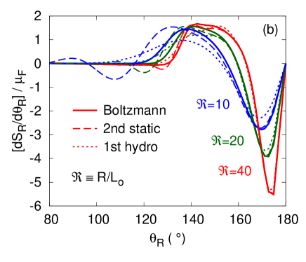
Figure 4: The angular distribution of (a) the energy density $[\rm{d}E_{R}/\rm{d}\theta_{R}]/\mu_{F}$ and (b) the energy flux $[\rm{d}S_{R}/\rm{d}\theta_{R}]/\mu_{F}$ given by the Boltzmann equation at distances $\mathfrak{R}=10,\,20,\,\mbox{and}\,40$. The Boltzmann results are compared with the first order and second order static hydrodynamics.

Figure 5: The angular distribution of (a) the energy density $[{\rm d}E_{R}/{\rm d}\theta_{R}]/\mu_{F}(v)$ and (b) the energy flux $[{\rm d}S_{R}/{\rm d}\theta_{R}]/\mu_{F}(v)$ given by the AdS/CFT correspondence at distances $\mathfrak{R}=5,\,10,\,\mbox{and}\,20$. The AdS/CFT results are compared with the first order and second order static hydrodynamics. Here ${L_{o}}=1/\pi T$ is the shear length and $\mu_{F}(v)=\gamma\sqrt{\lambda}\pi T^{2}/2$ is the heavy quark drag coefficient for the AdS/CFT.

Figure 6: The angular distribution of the energy density $[\rm{d}E_{R}/\rm{d}\theta_{R}]/\mu_{F}$ in (a) kinetic theory and (b) the AdS/CFT. The kinetic theory curves are plotted at distances $\mathfrak{R}=20,\,40$ while the AdS/CFT curves are plotted at distances $\mathfrak{R}=10,\,20$. The Boltzmann and AdS/CFT results are compared to the static and dynamic implementations of second order hydrodynamics (see text). The differences between the static and dynamic implementations of second order hydrodynamics reflects the size of neglected third order terms. Here ${L_{o}}$ is the shear length and $\mu_{F}(v)$ is the drag coefficient for each theory.

V Summary and Discussion

To keep this discussion self contained, we first recapitulate the problem and the corresponding notation. An infinitely heavy quark moves along the $z$ axis with velocity $v\simeq c$, depositing energy and disturbing the surrounding equilibrium plasma. We presented and compared the energy and momentum density distributions in two distinctly different plasmas – a weakly coupled QCD plasma described by kinetic theory and a strongly coupled ${\mathcal{N}}=4$ plasma described by the AdS/CFT correspondence. The steady state stress tensor distributions can be written in cylindrical coordinates and comoving coordinates (see Eqs 4 and 5). Fig. 1 and Fig. 2 exhibit the energy density $T^{00}$ and the magnitude of the Poynting vector $|{\bf S}|\equiv|T^{0i}|$ for kinetic theory and the ${\mathcal{N}}=4$ theory respectively. To compare these theories we measured all distances in terms of a length scale given by a combination of hydrodynamic parameters

$${L_{o}}\equiv\frac{\textstyle{\frac{4}{3}}\eta c}{(e+{\mathcal{P}})c_{s}^{2}}\,.$$

This length is of order the mean free path in kinetic theory and equals $1/\pi T$ for the AdS/CFT. In each theory we divided the stress tensor by the corresponding heavy quark drag coefficient $\mu_{F}(v)$ so that at asymptotically large distances (where ideal hydrodynamics is valid) the rescaled stress tensors are equal. At asymptotic distances both theories reproduce the “Mach cone” structure characteristic of ideal hydrodynamics, but these model plasmas differ at sub-asymptotic distances in their approach to this ideal hydrodynamic regime. In particular the Boltzmann theory is considerably less diffuse than the AdS/CFT. In kinetic theory the short distance response is reactive, and the sharp band seen in Fig. 2(a) (which is indicative of free streaming quasi-particles) is absent in Fig. 2(b). We will see that the response of the AdS/CFT closely follows the predictions of hydrodynamics at modest distances which is strongly damped by the shear viscosity at short distances. This difference between the two can also be seen quantitatively in Fig. 3 which compares the kinetic theory and AdS/CFT results by plotting the energy density and energy flux at concentric circles of radius $R$ in scaled units:

$$\mathfrak{R}=R/{L_{o}}\,.$$

The precise definitions of $dE_{R}/d\theta_{R}$ and ${\rm d}S_{R}/{\rm d}\theta_{R}$ is given by Eqs. 47, 48, and 49 respectively. As discussed in the previous paragraph, the AdS/CFT curves are considerably broader than the corresponding kinetic theory results for $\mathfrak{R}>5$.

Examining Fig. 3 a striking feature of the AdS result is the dramatic transition from hydrodynamic behavior at $\mathfrak{R}=5$ to vacuum physics at $\mathfrak{R}=1$ which is not present in the kinetic theory calculation. This transition was noted previously and suggested as a way to reveal the strong coupling dynamics experimentally Noronha et al. (2009). However, the absence of this transition in the weak coupling calculation reflects a limitation of the kinetic theory approximation to QCD rather than a distinguishable difference between the AdS/CFT correspondence and weakly coupled QCD. Certainly the quantum dynamics at $R\sim 1/\pi T$ can not be captured by the semi-classical kinetic theory results. It would be interesting to compute the stress tensor in this region in fixed order finite temperature perturbation theory to see if the dynamics of the two theories is similar at these length scales. As discussed in Section III using a short distance expansion Gubser and Pufu (2008); Yarom (2007), in the AdS/CFT calculation new length scales emerge at distances of order $1/\gamma^{1/2}\pi T$ and $1/\gamma^{3/2}\pi T$ which are not visible in Fig. 3. These scales have been associated with saturation physics Hatta et al. (2008); Dominguez et al. (2008).

Finally, we have analyzed the transition to the hydrodynamic regime in kinetic theory and the AdS/CFT. In particular we have determined the source appropriate for first and second order hydrodynamics in each theory, following in part a method outlined by Chesler and Yaffe Chesler and Yaffe (2008). This is elaborated in Section IV, and the precise source (which takes the form of derivatives of delta functions acting at the position of the quark) is given in Table 1. The source is constructed so that the hydrodynamics to a given order, together with a source at the same order, reproduces the stress tensor of the full theory up to higher order powers of $\ell_{\rm mfp}/R$. Fig. 8 given in Appendix B fits our extracted hydrodynamic source with a polynomial at small ${\bm{k}}$ and the superb agreement with our full numerical results justifies the source analysis of Section IV.

Fig. 4 compares first order and second order hydrodynamics to the kinetic theory results. Generally the second order theory provides only a minor improvement to the first order results until rather large radii, $\mathfrak{R}\mbox{~{}{\raisebox{1.72218pt}{$>$}} {\raisebox{-2.58334pt}{$\sim$}}~{}}40$. Indeed the behavior of the second order theory seems rather unphysical for $\mathfrak{R}\mbox{~{}{\raisebox{1.72218pt}{$<$}} {\raisebox{-2.58334pt}{$\sim$}}~{}}10$. This shows the limitations of second order hydrodynamics. Second order hydrodynamics is constructed to reproduce the full results order by order at asymptotic distances and is not constructed to describe the decay of non-equilibrium transients produced by the heavy quark.

The slow convergence of hydrodynamic expansion to the full results of kinetic theory can be contrasted with the rapid convergence seen in the AdS/CFT results in Fig. 5. In the AdS/CFT case we see that first (second) order hydrodynamics describes the full result at the 20% (4%) level for $\mathfrak{R}\simeq 5$. The agreement with hydrodynamics is not as good as described earlier by Chesler and Yaffe. This is because we are describing a quark moving with velocity $v=1$, and we have found that the deviation from equilibrium is noticeably larger than the $v=0.75$ quarks studied by these authors. In addition the energy density distributions show larger deviations from first order hydrodynamics and were not studied previously. However, once (important) second order hydrodynamic corrections are included, the agreement with hydrodynamics is remarkable already at modest $\mathfrak{R}$.

We should mention that we have used the “static” version of second hydrodynamics which specifies $\pi^{\mu\nu}$ with a constituent relation analogous to the first order constituent relation Baier et al. (2008). Israel-Stewart type equations rewrite and interpret the constituent relation as a dynamic equation using lower order equations of motion. This renders the system of equations hyperbolic and causal, but mixes orders in the gradient expansion. We have compared the static and the dynamic theories for the kinetic and AdS theories in Fig. 6. Generally the Israel-Stewart type resummations do not lead to a significant improvement. Indeed, at smaller $\mathfrak{R}$ than shown in Fig. 6  Israel-Stewart type resummations can lead to spurious shocks which are not reproduced by the full result. The differences between the static and dynamic theories gives an estimate of higher order terms, and this difference is smaller in AdS/CFT than in kinetic theory at the same $\mathfrak{R}$.

Clearly, the convergence to the hydrodynamic limit is significantly faster in the ${\mathcal{N}}=4$ theory relative to kinetic theory, even when lengths are measured in the scaled units described by $\mathfrak{R}$. We remark that in the AdS/CFT the second order hydrodynamic parameter $\tau_{\pi}$ is a factor of $2.5$ smaller in scaled units than the corresponding kinetic theory parameter,

$$\frac{\tau_{\pi}}{\eta/sT}= 6.32\,,$$ (Kinetic Theory) (67)

$$\frac{\tau_{\pi}}{\eta/sT}= 4-2\log(2)\simeq 2.61\,.$$ (AdS/CFT) (68)

Based on these coefficients, it is natural to expect that the convergence to the hydrodynamic limit is faster for the ${\mathcal{N}}=4$ theory than the corresponding kinetic theory. In theories based on quasi-particles and kinetic theory it is difficult to reduce the value of $\tau_{\pi}$ in scaled units significantly York and Moore (2009). Thus, it would seem that our principal result of this study is reasonably generic. Specifically, based on the model theories studied in this work we expect theories without quasiparticles to approach the hydrodynamic limit several times faster (in scaled units) than theories based on a quasiparticle description. From a practical perspective of applying hydrodynamics to various almost equilibrium phenomena of heavy ion physics (e.g. the hydrodynamic flow due to jets and other local disturbances) this factor of two can be quite important.

Acknowledgments:

P. Chesler is supported by a Pappalardo Fellowship at MIT. D. Teaney and J. Hong are supported in part by the Sloan Foundation and by the Department of Energy through the Outstanding Junior Investigator program, DE-FG-02-08ER4154.

Appendix A The kinetic theory source in a leading-log approximation

The source of non-equilibrium gluons arises as gluons scatter off the heavy quark, $g+{\rm Q}\rightarrow g+{\rm Q}$. The squared matrix element for this process is

$$\left|{\cal M}\right|^{2}=\left[\frac{g^{4}C_{F}N_{c}}{2d_{A}}\right]16\left[\frac{2(K\cdot P)^{2}}{Q^{4}}-\frac{M^{2}}{Q^{2}}+\frac{M^{2}}{4(K\cdot P)^{2}}\right]\,,$$ (69)

where $K$ is the heavy quark momentum, $P$ is the gluon momentum, $Q=P^{\prime}-P$ is the four momentum transferred to the gluon, and we have averaged over the colors and spins of the external gluon. In a leading log approximation only the (first) most singular term is kept. The source of non-equilibrium gluons of momentum ${\bm{p}}$ is obtained from the Boltzmann collision integral for the $g+Q\rightarrow g+Q$ process

$$S(t,{\bm{x}},{\bm{p}})= S({\bm{p}})\delta^{3}({\bm{x}}-{\bm{v}}t)$$

$$= -\int_{kp^{\prime}k^{\prime}}\frac{|{\cal M}|^{2}}{16k^{0}k^{{}^{\prime}0}pp^{\prime}}(2\pi)^{4}\delta^{4}(P_{tot})[f_{p}f_{k}(1+f_{p^{\prime}})(1+f_{k^{\prime}})-f_{p^{\prime}}f_{k^{\prime}}(1+f_{p})(1+f_{k})]\,,$$ (70)

where the heavy quark distribution $f_{k}=(2\pi)^{3}\delta^{3}({\bm{k}}-{\bm{k}}_{H})\delta^{3}({\bm{x}}-{\bm{v}}t)$ is out of equilibrium.

We expand the source in a spherical harmonic basis in the $(x,y,z)$ coordinate system

$$S({\bm{p}})= \sum_{l,m}S_{lm}(p)H_{lm}(\hat{{\bm{p}}};zx)=\sqrt{\frac{2l+1}{4\pi}}\sum_{l}S_{l0}(p)P_{l}(\cos\theta_{{\bm{p}}{\bm{k}}})\,,$$ (71)

and note that the $S_{lm}$ vanishes for non-zero $m$ due to the azimuthal symmetry of the problem. Using the orthogonality of $P_{l}(\cos\theta_{{\bm{p}}{\bm{k}}})$ and the phase-space parameterization and kinematic approximations used to analyze the energy loss of heavy quarks Moore and Teaney (2005), the expansion coefficients can be written

$$S_{l0}(p)=-\sqrt{\frac{2l+1}{4\pi}}\int_{0}^{\infty}dq\int_{-vq}^{vq}\frac{d\omega}{v}\int\frac{d\phi}{2\pi}P_{l}(\cos\theta_{{\bm{p}}{\bm{k}}})\frac{|\mathcal{M}|^{2}}{16p^{2}(k^{0})^{2}}\left[f_{p}(1+f_{p+\omega})-f_{p-\omega}(1+f_{p})\right]\,,$$ (72)

where $\omega$ is the energy transfer, ${\bm{q}}={\bm{p}}^{\prime}-{\bm{p}}$ is the three momentum transfer, and $\phi$ is the azimuthal angle. The matrix elements in this parameterization are

$$\frac{|\mathcal{M}|^{2}}{16p^{2}(k^{0})^{2}}=\left[\frac{g^{4}C_{F}N_{c}}{2d_{A}}\right]\frac{2(1-v\cos\theta_{{\bm{k}}{\bm{p}}})^{2}}{(q^{2}-\omega^{2})^{2}}\,,$$ (73)

where $\cos\theta_{{\bm{k}}{\bm{p}}}$ is expressed in terms of the integration variables, $\omega$, $q$ and $\phi$ Moore and Teaney (2005). Now we consistently expand out the integrand to quadratic order in $\omega/T$ and $q/T$. This includes three types of terms: (1) an expansion of the distribution functions to quadratic order, (2) an expansion of the angle $\cos\theta_{pk}$ to linear order in $q/T$ and (3) an expansion of the Legendre polynomial to linear order, $P_{l}(x+\delta x)\simeq P_{l}(x)+P_{l}^{\prime}(x)\,\delta x$. With the full expansion we explicitly integrate over the azimuthal angle $\phi$ and the energy $\omega$, observing empirically that all harmonics vanish for $l>1$ when the velocity is lightlike. Further, the $l=0$ and $l=1$ harmonics can be done analytically leading to a simple answer recorded in Eq. (19)

$$S_{00}(p) = \frac{1}{\sqrt{4\pi}T^{2}}\,\left[\frac{g^{4}C_{F}N_{c}}{2d_{A}}\right]\,\log\left(\frac{T}{m_{D}}\right)f_{p}(1+f_{p})\left(-\frac{2T}{p}+1+2f_{p}\right)\,,$$ (74a)

$$S_{10}(p) = \frac{1}{\sqrt{12\pi}T^{2}}\,\left[\frac{g^{4}C_{F}N_{c}}{2d_{A}}\right]\,\log\left(\frac{T}{m_{D}}\right)f_{p}(1+f_{p})(1+2f_{p})\,,$$ (74b)

The leading-log simplifications described in this paragraph were observed previously when computing the shear viscosity.

Appendix B Numerical Details about Kinetic theory and the Fourier Transform

The goal of this appendix is to give some of the details of how the stress tensor is computed in kinetic theory. Most of the notation and strategy follows an appendix of Ref. Hong and Teaney (2010) and this reference should be consulted for the full details.

The linearized Boltzmann equation in Fourier space reads

$$(-i\omega+i{\bm{v}}_{p}\cdot{\bm{k}})\delta f(\omega,{\bm{k}},{\bm{p}})=C[\delta f,{\bm{p}}]+2\pi S({\bm{p}})\delta(\omega-{\bm{v}}\cdot{\bm{k}})\,,$$ (75)

where ${\bm{v}}_{\bm{p}}=\hat{\bm{p}}$ is the particle velocity and the vector ${\bm{k}}$ in the laboratory coordinate system is

$${\bm{k}}=(k^{x},k^{y},k^{z})=k(\sin\theta_{\bm{k}}\cos\varphi_{k},\,\sin\theta_{\bm{k}}\sin\varphi_{k},\,\cos\theta_{\bm{k}})\,.$$ (76)

In order to solve Eq. (75) numerically, it is convenient to introduce the Fourier coordinate system $(x^{\prime},y^{\prime},z^{\prime})$ where $\hat{{\bm{z}}}^{\prime}$ points along the Fourier momentum ${\bm{k}}$

$$\hat{\bm{x}}^{\prime}= \frac{k}{k_{T}}\hat{{\bm{k}}}\times(\hat{{\bm{v}}}\times\hat{\bm{k}})\,,$$ (77)

$$\hat{\bm{y}}^{\prime}= \frac{k}{k_{T}}\hat{{\bm{v}}}\times\hat{\bm{k}}\,,$$ (78)

$$\hat{\bm{z}}^{\prime}= \hat{\bm{k}}\,.$$ (79)

Following our previous work Hong and Teaney (2010) we re-express the source and ultimately the solution $\delta f$ in terms of real spherical harmonics with respect to the $\hat{{\bm{x}}}^{\prime},\hat{{\bm{y}}}^{\prime},\hat{{\bm{z}}}^{\prime}$ coordinate system:

$$H_{lm}(\hat{\bm{p}};z^{\prime}x^{\prime})=N_{lm}P_{l|m|}(\cos\theta_{\bm{p}})\times\left\{\begin{array}[]{ll}1&\mbox{\quad for $m=0$}\\ \sqrt{2}\cos m\varphi_{\bm{p}}&\mbox{\quad for $m>0$ }\\ \sqrt{2}\sin|m|\varphi_{\bm{p}}&\mbox{\quad for $m<0$ }\\ \end{array}\right.\,,$$ (80)

where $N_{lm}$ is a normalization factor Hong and Teaney (2010). We note that the unit vector $\hat{\bm{p}}$ has the following components

$$\hat{{\bm{p}}}^{x^{\prime}}=\sqrt{\frac{4\pi}{3}}H_{11}(\hat{\bm{p}};z^{\prime}x^{\prime})\,,\qquad\hat{{\bm{p}}}^{y^{\prime}}=\sqrt{\frac{4\pi}{3}}H_{1,-1}(\hat{\bm{p}};z^{\prime}x^{\prime})\,,\qquad\hat{{\bm{p}}}^{z^{\prime}}=\sqrt{\frac{4\pi}{3}}H_{10}(\hat{\bm{p}};z^{\prime}x^{\prime})\,.$$ (81)

Since the distribution function $\delta f$ is independent of the azimuthal angle of ${\bm{k}}$ with respect to the original $x,y,z$ coordinate system, we will choose this azimuthal angle $\varphi_{k}$ to be zero so that ${\bm{k}}$ lies in the $x,z$ plane. Then in the $(x^{\prime},y^{\prime},z^{\prime})$ coordinate system the vector ${\bm{v}}$ has the components

$$\hat{{\bm{v}}}=(v^{x^{\prime}},v^{y^{\prime}},v^{z^{\prime}})=(\sin\theta,0,\cos\theta)\,,$$

and

$$\hat{{\bm{v}}}\cdot\hat{{\bm{p}}}=\sqrt{\frac{4\pi}{3}}\Big{(}\cos\theta\,H_{10}(\hat{\bm{p}};z^{\prime}x^{\prime})+\sin\theta\,H_{11}(\hat{\bm{p}};z^{\prime}x^{\prime})\Big{)}\,.$$ (82)

The steady state solution to the linearized Boltzmann equation is also expanded in the spherical harmonics defined above

$$\delta f(\omega,{\bm{k}},{\bm{p}})=\sum_{lm}2\pi\delta(\omega-{\bm{v}}\cdot{\bm{k}})n_{p}(1+n_{p})\chi_{lm}(p,{\bm{k}})H_{lm}(\hat{{\bm{p}}};z^{\prime}x^{\prime})\,.$$ (83)

and the Boltzmann equation for $\chi_{lm}$ becomes

$$\left(-i\omega\delta_{ll^{\prime}}+ikC_{ll^{\prime}}^{m}\right)p^{2}n_{p}(1+n_{p})\chi_{l^{\prime}m}=C_{lm}[\delta f,{\bm{p}}]+{\mathcal{H}}p^{2}n_{p}(1+n_{p})\frac{\mu_{A}}{T}{\mathcal{S}}_{lm}(p,\theta)\,,$$ (84)

where the $m$ index is not summed over. Here $C_{ll^{\prime}}^{m}$ is a Clebsch Gordan coefficient Hong and Teaney (2010), $C_{lm}[\delta f,{\bm{p}}]$ is the collision integral in this basis, the normalization coefficient is

$${\mathcal{H}}=\frac{\mu_{F}}{T^{3}d_{A}\mu_{A}}\,,$$ (85)

and the source is

$${\mathcal{S}}_{lm}(p,\theta)=\frac{1}{2\xi_{B}/T^{3}}\Big{[}\left(\frac{-2T}{p}+1+2n_{p}\right)\sqrt{4\pi}\delta_{l0}\delta_{m0}\\ +\sqrt{\frac{4\pi}{3}}\left(1+2n\right)\left(\delta_{l1}\delta_{m0}\cos\theta+\delta_{l1}\delta_{m1}\sin\theta\right)\Big{]}\,.$$ (86)

For each value of $(k_{x},k_{z})$ (in units of $\mu_{A}/T$) the linear equations are solved for $F_{lm}\equiv\chi_{lm}/{\mathcal{H}}$. Due to rotational invariance of the collision operator around the ${\bm{k}}$ axis, the matrix equation does not mix harmonics with different magnetic quantum numbers, i.e. the collision operator is diagonal in $m$. Thus, the matrix equation in $l,l^{\prime}$ is solved for $m=1$ and $m=0$ separately. Harmonics with $m>1$ are not sourced by the motion of the quark in a leading log approximation.

After solving for $\delta f(\omega,{\bm{k}},{\bm{p}})$, the energy and momentum excess due to the moving quark can be computed using the kinetic theory

$$\delta T^{0\mu}(\omega,{\bm{k}})=2d_{A}\int\frac{{\rm d}^{3}{\bm{p}}}{(2\pi)^{3}}\,p^{\mu}\delta f(\omega,{\bm{k}},{\bm{p}})\,,$$ (87)

where $T^{0\mu}(\omega,{\bm{k}})$ is proportional to $2\pi\delta(\omega-{\bm{v}}\cdot{\bm{k}})$

$$\delta T^{0\mu}(\omega,{\bm{k}})\equiv 2\pi\delta(\omega-{\bm{v}}\cdot{\bm{k}})\tilde{T}^{0\mu}(k_{z},k_{T})\,.$$ (88)

The relationship between the $(x,y,z)$ and the $(x^{\prime},y^{\prime},z^{\prime})$ coordinate system is

$$\delta T^{0x}(\omega,{\bm{k}})= \cos\theta\,\delta T^{0x^{\prime}}(\omega,{\bm{k}})-\sin\theta\,\delta T^{0z^{\prime}}(\omega,{\bm{k}})$$ (89)

$$\delta T^{0y}(\omega,{\bm{k}})= 0$$ (90)

$$\delta T^{0z}(\omega,{\bm{k}})= \sin\theta\,\delta T^{0x^{\prime}}(\omega,\mathbf{k})+\cos\theta\,\delta T^{0z^{\prime}}(\omega,\mathbf{k})\,,$$ (91)

In presenting these formulas we have taken ${\bm{k}}$ in the $x,z$ plane, i.e. $\varphi_{k}=0$. More generally rotational invariance dictates that $(T^{0x},T^{0y})$ is proportional to $\hat{\bm{k}}_{T}$

$$\delta\tilde{T}^{0x}({\bm{k}})= \delta\tilde{T}^{0k_{T}}(k_{z},k_{T})\cos\varphi_{k}\,,$$ (92)

$$\delta\tilde{T}^{0y}({\bm{k}})= \delta\tilde{T}^{0k_{T}}(k_{z},k_{T})\sin\varphi_{k}\,,$$ (93)

and the preceding discussion with $\varphi_{k}=0$ suffices to determine $T^{0k_{T}}(k_{z},k_{T})$.

The stress tensor is tabulated in the $k_{z},k_{T}$ plane and then Fourier transforms can be used to compute the stress tensor in coordinate space

$$\delta T^{0\mu}(t,{\bm{x}})=\int_{-\infty}^{\infty}\frac{{\rm d}\omega}{2\pi}\int\frac{{\rm d}^{3}{\bm{k}}}{(2\pi)^{3}}e^{-i\omega t+i{\bm{k}}\cdot{\bm{x}}}\,\delta T^{0\mu}(\omega,{\bm{k}})\,.$$ (94)

Employing the familiar identity

$$e^{ik_{T}x_{T}\cos(\varphi_{r}-\varphi_{k})}=J_{0}(k_{T}x_{T})+2\sum_{n}i^{n}J_{n}(k_{T}x_{T})\cos(n(\varphi_{r}-\varphi_{k}))\,,$$ (95)

it is not difficult to show that

$$\delta T^{00}(x_{L},x_{T})= \int_{0}^{\infty}\frac{k_{T}{\rm d}k_{T}}{2\pi}J_{0}(k_{T}x_{T})\,\int_{-\infty}^{\infty}\frac{{\rm d}k_{z}}{2\pi}e^{ik_{z}z}\,\delta\tilde{T}^{00}(k_{z},k_{T})\,,$$ (96a)

$$\delta T^{0x_{T}}(x_{L},x_{T})= \int_{0}^{\infty}\frac{k_{T}{\rm d}k_{T}}{2\pi}J_{1}(k_{T}x_{T})\int_{-\infty}^{\infty}\frac{{\rm d}k_{z}}{2\pi}e^{ik_{z}z}i\,\delta\tilde{T}^{0k_{T}}(k_{z},k_{T})\,,$$ (96b)

$$\delta T^{0z}(x_{L},x_{T})= \int_{0}^{\infty}\frac{k_{T}{\rm d}k_{T}}{2\pi}J_{0}(k_{T}x_{T})\int_{-\infty}^{\infty}\frac{{\rm d}k_{z}}{2\pi}e^{ik_{z}z}\,\delta\tilde{T}^{0k}(k_{z},k_{T})\,.$$ (96c)

The Fourier integrals in Eq. (96) are not particularly easy. In order to get a convergent integral, we first multiply the numerical data by a window function which eliminates the contributions of high frequency modes. For kinetic theory results, a sample window function is

$$W(k)=\frac{1}{2}\bigg{[}1-\mbox{erf}\left((k-k_{\rm max})/\sigma\right)\bigg{]}.$$ (97)

with $k_{\rm max}=7.5\mu_{A}/T$ and $\sigma=3.5\mu_{A}/T$ while for the AdS/CFT the $k_{\rm max}$ and $\sigma$ was considerably larger, $k_{\rm max}=80\pi T$ and $\sigma=60\pi T$. We computed the integrals in Eq. (96) using two methods. The first method used brute force summation to compute these integrals. In the second method we re-parameterized the stress tensor by the source functions $\phi_{v}$ and $\phi_{k}$ used in the hydrodynamic analysis. Specifically, we define the functions $\phi_{v}({\bm{k}})$ and $\phi_{k}$ by the equations

$$\delta T^{0x^{\prime}}(\omega,{\bm{k}})= \frac{i\sin\theta\phi_{v}({\bm{k}})}{\omega+iDk^{2}}\,2\pi\mu_{F}\,\delta(\omega-k\cos\theta)\,,$$ (98)

$$\delta T^{0z^{\prime}}(\omega,{\bm{k}})= \frac{i\left(\omega\cos\theta\phi_{v}({\bm{k}})+c^{2}(k)k\right)-k\omega\phi_{k}({\bm{k}})}{\omega^{2}-c^{2}(k)k^{2}+i\Gamma_{s}\omega k^{2}}\,2\pi\mu_{F}\,\delta(\omega-k\cos\theta)\,,$$ (99)

where $c^{2}(k)=c_{s}^{2}(1+\tau_{\pi}\Gamma_{s}k^{2})$ and $T^{00}(\omega,{\bm{k}})$ is determined by energy-momentum conservation. This reparametrization is used for all values of the Fourier momentum ${\bm{k}}$. Such a reparametrization is useful because, in contrast to $T^{0x^{\prime}}$ and $T^{0z^{\prime}}$, the functions $\phi_{v}({\bm{k}})$ and $\phi_{k}({\bm{k}})$ are smooth and can be easily and accurately interpolated. Then the integrals are computed using Gaussian quadrature with break points at the hydrodynamic poles. The brute force summation and the more sophisticated numerical scheme give the same answer at the 1% level and are independent of the cutoff parameters.

Appendix C Details on the Hydrodynamic Source in Kinetic Theory and the AdS/CFT

The purpose of this appendix is to explain in somewhat greater detail how the coefficients given in Table 1 are computed for both kinetic theory and the AdS/CFT. In the process, we will exhibit several fits to our numerical results. The quality of these fits indicates that the deviation of the stress tensor from its hydrodynamic form at small ${\bm{k}}$ and $\omega$ is well described by a multivariate polynomial and justifies the hydrodynamic analysis of Section IV. We will first discuss the AdS/CFT theory and then indicate how the analysis can be applied to kinetic theory.

C.1 AdS/CFT

The applicability of second order hydrodynamics to the AdS/CFT has been questioned based on the analytic structure of retarded stress tensor correlators in the lower half plane Noronha and Denicol (2011); Denicol et al. (2010). However, provided second order hydrodynamics is used to describe the behavior of hydrodynamic modes (i.e a pole in the retarded Green function arbitrarily close to the real axis), rather than to model the decay of non-hydrodynamic modes or transients (i.e. additional analytic structure in the lower half plane), second order hydrodynamics is applicable to this strongly coupled theory. This appendix serves to clarify this points.

After computing the exact stress tensor of the full AdS/CFT theory we define the functions $\phi_{v}({\bm{k}})$ and $\phi_{k}({\bm{k}})$ as in Eq. (98). This would seem to be simply a reparametrization of the original numerical data on $T^{0x^{\prime}}$ and $T^{0z^{\prime}}$ with two functions $\phi_{v}({\bm{k}})$ and $\phi_{k}({\bm{k}})$. However, as we will see, the functions $\phi_{v}({\bm{k}})$ and $\phi_{k}({\bm{k}})$ are analytic functions of ${\bm{k}}$ while the original fields have poles arbitrarily close to the real axis as ${\bm{k}}\rightarrow 0$, see Eq. (65). The purpose of first and second order hydrodynamics is to describe the location of these poles. First order hydrodynamics determines the pole location to first order in $k\ell_{\rm mfp}$, but neglects terms of order $(k\ell_{\rm mfp})^{2}$ which are captured by second order hydrodynamics. It should be emphasized that the pole shift is a consequence of modifying the ideal hydrodynamic equations of motion by powers of $k\ell_{\rm mfp}$ rather than modifying the source. Since, the ideal solution has a hydrodynamic pole at $\omega=c_{s}k$ modifying the equations of motion does not simply correct the solution by simple powers $k\ell_{\rm mfp}$ close to the pole. We will determine the source functions $\phi_{v}({\bm{k}})$ and $\phi_{k}({\bm{k}})$ using first and second order hydrodynamics. Specifically, we determine $\phi_{v}({\bm{k}})$ and $\phi_{k}({\bm{k}})$ using Eq. (98) (with the same numerical data for the full stress tensor $T^{0x^{\prime}}$ and $T^{0z^{\prime}}$), but in the first order case we set the second order transport coefficient to zero in these equations, $\tau_{\pi}\rightarrow 0$.

Since the source functions $\phi_{v}$ and $\phi_{k}$ are functions of $k$ and $\omega=k\cos\theta$, we can expand these functions in Fourier series

$$\phi_{v}({k},\cos\theta)\equiv\phi_{v;0}({k})+2\phi_{v;1}({k})\cos\theta+2\phi_{v;2}({k})\cos 2\theta+\ldots.$$ (100)

$$\pi T\phi_{k}({k},\cos\theta)\equiv\phi_{k;0}({k})+2\phi_{k;1}({k})\cos\theta+2\phi_{k;2}({k})\cos 2\theta+\ldots.$$ (101)

In Fig. 7 we plot the terms of the Fourier series $\phi_{v;n}(k)$ and $\phi_{k;n}(k)$ and fit these functions with a simple power law, $k^{\alpha}$.

Figure 7: Hydrodynamic fits to the AdS/CFT source functions $\phi_{v}\equiv 1+\Delta\phi_{v}$ and $\pi T\phi_{k}=-\frac{1}{3}+\Delta\phi_{k}$ at small $k$ (see the text surrounding Eq. (100)). The Fourier coefficients displayed in this figure have been multiplied by a factor indicated in parentheses to increase visibility, and are fit with the functional form $Ck^{\alpha}$. The dashed lines and open symbols have non-integer fit-powers and lie beyond the description of hydrodynamics to the specified order, i.e. the fit is not expected to work. (a) The $n=0$, $n=1$, and $n=2$ Fourier coefficients of $\phi_{v}$. (b) The $n=0$, $n=1$, and $n=2$ Fourier coefficients of $\phi_{k}$, when $\phi_{k}$ is extracted using first order hydrodynamics. (c) Same as (b), but for second order hydrodynamics.

As we see from the fit, $\phi_{v}$ is well described by a quadratic polynomial at small $k$

$$\phi_{v;0}(k)=1-0.1643\left(\frac{k}{\pi T}\right)^{2}\,,\qquad\phi_{v;1}=0.5i\left(\frac{k}{\pi T}\right)\,,\qquad\phi_{v;2}=0.0870\left(\frac{k}{\pi T}\right)^{2}\,.$$ (102)

For first order hydrodynamics the terms of quadratic order can be neglected. Our numerical result for $\phi_{v;1}$ is nicely consistent with the first order analytic result Ref. Chesler and Yaffe (2007).)

Now we examine $k\phi_{k}$ using first and second order hydrodynamics. When first order hydrodynamics is used the source function is not well described by a polynomial (see Fig. 7(b)). However, we see that $k\phi_{k}$ decreases faster than $k$ (as $k^{1.52}$ for $n=1$), and therefore $k\phi_{k}$ can be neglected in a first order hydrodynamic analysis of the long wavelength response to the heavy quark. A concerned reader might worry that the resulting source function $k\phi_{k}$ is not well described by a quadratic polynomial, and incorrectly conclude a local source for hydrodynamics can not be constructed beyond linear order. However, when second order hydrodynamics is used to extract the source through quadratic order (as is appropriate), $k\phi_{k}$ is well described by the quadratic polynomial – see the linear fit in Fig. 7(c) for $\phi_{k;1}$. Numerically we find

$$\phi_{k;0}=-\frac{1}{3}\,,\qquad\phi_{k;1}=0.11i\frac{k}{\pi T}\,,$$ (103)

up to non-analytic terms that fall faster than $k^{2}$. (These non-analytic terms could be removed by pushing the hydrodynamic analysis to third order.) In summary, we see that using second order hydrodynamics neatly removes the non-analytic behavior seen in the first order source, and then the source for second order hydrodynamics is then well described by a quadratic polynomial. The coefficient $\tau_{\pi}$ which shifts the hydrodynamic pole is universal – it was determined through an analysis of two point functions Baier et al. (2008), and the same coefficient determines the long distance response to the disturbance produced by a heavy quark. By contrast the source functions $\phi_{v}$ and $\phi_{k}$ are not universal but depend on the particular way in which the heavy quark couples to hydrodynamic modes. Using the fits in Eq. (102) and Eq. (103) (and the relation between $\phi_{v},\phi_{k}$ and $\phi_{1}$,$\phi_{2}$ given in Eq. (62)), we parametrize this source by three numbers to quadratic order which are given in Table 1.

C.2 Kinetic Theory

As in the previous appendix, we define the functions $\phi_{v}$ and $\phi_{k}$ from the exact stress tensor (Eq. (98)), and again expand these functions in Fourier series as in Eq. (100), but, as is appropriate for the kinetic theory calculation, $\pi T\phi_{k}$ is replaced with $(\mu_{A}/T)\phi_{k}$ . Then the Fourier coefficients are fit with a polynomial which are shown in Fig. 8. It was verified that the other Fourier coefficients of $\phi_{v}$ and ${k}\phi_{k}$ that are not shown decrease faster than ${k}^{2}$ and thus lie outside of the hydrodynamic analysis which is restricted to second order inclusive. Examining the fits shown in Fig. 8, we see that the parameterization

$$\phi_{v;0}= 1+1.66(1)\left(\frac{kT}{\mu_{A}}\right)^{2}\,,$$ (104)

$$\phi_{k;1}= -\frac{1}{6}1.66(1)i\frac{kT}{\mu_{A}}\,,$$ (105)

describes our numerical data at small $k$ and $\omega=k\cos\theta$ quite well. The fact that $\phi_{v;0}$ and $\phi_{k;1}$ have the same fit coefficient (up to a symmetry factor of $1/6$) is a consequence of the hydrodynamic analysis of Section IV. Comparing the fit with the functional form given in the text (Eq. (62)), we see that we have a non-zero $\phi_{2}^{(0,0)}$ (which is recorded in Table  1), but the coefficients $\phi_{1}^{(0,0)}$ and $\phi_{1}^{(1,0)}$ seem to vanish. In fact $\phi_{1}(\omega,k^{2})$ vanishes to all orders in $\omega,k$ as we will now show.

Figure 8: (a) A polynomial fit to the source function $\phi_{v;0}$ defined in Eq. (100). The fit result is recorded in Eq. (104). (b) Using the fit coefficient from $(a)$, a prediction is made $\phi_{k;1}$ (see Eq. (104)) using the analysis of Section IV.

To this end we can return to the analysis given in Section IV. For a given ${\bm{k}}$, we expect that there is a non-zero component of $T^{ij}(\omega,{\bm{k}})$ which transforms as a spin two tensor under azimuthal rotations around the ${\bm{k}}$ axis. Examining the decomposition of $\tau^{ij}\equiv T^{ij}-T^{ij}_{\rm hydro}$ into tensor structures (Eq. (59)), and noting that hydrodynamics does not yield such a spin two tensor, we see that this spin two component of $T^{ij}$ determines $\left[v^{i}v^{j}-\frac{1}{3}v^{2}\delta^{ij}\right]\phi_{1}$, since this is the only tensor structure of $\tau^{ij}$ that has a spin two component under azimuthal rotations around ${\bm{k}}$. Examining the source for the Boltzmann equation given in Eq. (86) of Appendix B we see that the specific form of the source does not excite the spin two (i.e. $m=2$) components of the distribution function $\delta f$. Thus, since the Boltzmann equation does not mix harmonics of different spin, the spin two component of the stress tensor vanishes and so does $\phi_{1}$. This approximate symmetry is specific to the simplified form of the source which arises in a leading-log approximation and is not expected to hold more generally.

References

- Teaney (2009) Derek A. Teaney, “Viscous Hydrodynamics and the Quark Gluon Plasma,” (2009), arXiv:0905.2433 [nucl-th] .
- Blaizot et al. (2003) J.P. Blaizot, E. Iancu, and A. Rebhan, “On the apparent convergence of perturbative QCD at high temperature,” Phys.Rev. D68, 025011 (2003), arXiv:hep-ph/0303045 [hep-ph] .
- Andersen et al. (2011a) Jens O. Andersen, Lars E. Leganger, Michael Strickland, and Nan Su, “Three-loop HTL QCD thermodynamics,” JHEP 1108, 053 (2011a), arXiv:1103.2528 [hep-ph] .
- Andersen et al. (2011b) Jens O. Andersen, Lars E. Leganger, Michael Strickland, and Nan Su, “The QCD trace anomaly,” (2011b), * Temporary entry *, arXiv:1106.0514 [hep-ph] .
- Policastro et al. (2001) G. Policastro, D.T. Son, and A.O. Starinets, “The Shear viscosity of strongly coupled N=4 supersymmetric Yang-Mills plasma,” Phys.Rev.Lett. 87, 081601 (2001), arXiv:hep-th/0104066 [hep-th] .
- Kovtun et al. (2005) P. Kovtun, D.T. Son, and A.O. Starinets, “Viscosity in strongly interacting quantum field theories from black hole physics,” Phys.Rev.Lett. 94, 111601 (2005), an Essay submitted to 2004 Gravity Research Foundation competition, arXiv:hep-th/0405231 [hep-th] .
- Stoecker (2005) Horst Stoecker, “Collective flow signals the quark gluon plasma,” Nucl.Phys. A750, 121–147 (2005), arXiv:nucl-th/0406018 [nucl-th] .
- Casalderrey-Solana et al. (2005) J. Casalderrey-Solana, E.V. Shuryak, and D. Teaney, “Conical flow induced by quenched QCD jets,” J.Phys.Conf.Ser. 27, 22–31 (2005), arXiv:hep-ph/0411315 [hep-ph] .
- Gubser et al. (2008) Steven S. Gubser, Silviu S. Pufu, and Amos Yarom, “Sonic booms and diffusion wakes generated by a heavy quark in thermal AdS/CFT,” Phys. Rev. Lett. 100, 012301 (2008), arXiv:0706.4307 [hep-th] .
- Yarom (2007) Amos Yarom, “The High momentum behavior of a quark wake,” Phys.Rev. D75, 125010 (2007), arXiv:hep-th/0702164 [hep-th] .
- Chesler and Yaffe (2007) Paul M. Chesler and Laurence G. Yaffe, “The wake of a quark moving through a strongly-coupled supersymmetric Yang-Mills plasma,” Phys. Rev. Lett. 99, 152001 (2007), arXiv:0706.0368 [hep-th] .
- Chesler and Yaffe (2008) Paul M. Chesler and Laurence G. Yaffe, “The Stress-energy tensor of a quark moving through a strongly-coupled N=4 supersymmetric Yang-Mills plasma: Comparing hydrodynamics and AdS/CFT,” Phys.Rev. D78, 045013 (2008), arXiv:0712.0050 [hep-th] .
- Neufeld (2008) R.B. Neufeld, “Fast Partons as a Source of Energy and Momentum in a Perturbative Quark-Gluon Plasma,” Phys.Rev. D78, 085015 (2008), arXiv:0805.0385 [hep-ph] .
- Adare et al. (2008) A. Adare et al. (PHENIX Collaboration), “Dihadron azimuthal correlations in Au+Au collisions at s(NN)**(1/2) = 200-GeV,” Phys.Rev. C78, 014901 (2008), arXiv:0801.4545 [nucl-ex] .
- Abelev et al. (2009) B. I. Abelev et al. (STAR), “Indications of Conical Emission of Charged Hadrons at RHIC,” Phys. Rev. Lett. 102, 052302 (2009), arXiv:0805.0622 [nucl-ex] .
- Alver and Roland (2010) B. Alver and G. Roland, “Collision geometry fluctuations and triangular flow in heavy-ion collisions,” Phys.Rev. C81, 054905 (2010), arXiv:1003.0194 [nucl-th] .
- Takahashi et al. (2009) J. Takahashi, B.M. Tavares, W.L. Qian, R. Andrade, F. Grassi, et al., “Topology studies of hydrodynamics using two particle correlation analysis,” Phys.Rev.Lett. 103, 242301 (2009), arXiv:0902.4870 [nucl-th] .
- Sorensen (2010) Paul Sorensen, “Implications of space-momentum correlations and geometric fluctuations in heavy-ion collisions,” J.Phys.G G37, 094011 (2010), arXiv:1002.4878 [nucl-ex] .
- Lin et al. (2005) Zi-Wei Lin, Che Ming Ko, Bao-An Li, Bin Zhang, and Subrata Pal, “A Multi-phase transport model for relativistic heavy ion collisions,” Phys.Rev. C72, 064901 (2005), arXiv:nucl-th/0411110 [nucl-th] .
- Ma et al. (2006) G.L. Ma, S. Zhang, Y.G. Ma, H.Z. Huang, X.Z. Cai, et al., “Di-hadron azimuthal correlation and mach-like cone structure in parton/hadron transport model,” Phys.Lett. B641, 362–367 (2006), arXiv:nucl-th/0601012 [nucl-th] .
- Chaudhuri and Heinz (2006) A. K. Chaudhuri and Ulrich Heinz, “Effect of jet quenching on the hydrodynamical evolution of QGP,” Phys. Rev. Lett. 97, 062301 (2006), arXiv:nucl-th/0503028 .
- Casalderrey-Solana et al. (2006) J. Casalderrey-Solana, E.V. Shuryak, and D. Teaney, “Hydrodynamic flow from fast particles,” (2006), arXiv:hep-ph/0602183 [hep-ph] .
- Chatrchyan et al. (2011) Serguei Chatrchyan et al. (CMS Collaboration), “Observation and studies of jet quenching in PbPb collisions at nucleon-nucleon center-of-mass energy = 2.76 TeV,” Phys. Rev. C84, 024906 (2011), arXiv:1102.1957 [nucl-ex] .
- Gubser and Pufu (2008) Steven S. Gubser and Silviu S. Pufu, “Master field treatment of metric perturbations sourced by the trailing string,” Nucl. Phys. B790, 42–71 (2008), arXiv:hep-th/0703090 .
- Neufeld (2009) R.B. Neufeld, “Mach cones in the quark-gluon plasma: Viscosity, speed of sound, and effects of finite source structure,” Phys.Rev. C79, 054909 (2009), arXiv:0807.2996 [nucl-th] .
- Hong and Teaney (2010) Juhee Hong and Derek Teaney, “Spectral densities for hot QCD plasmas in a leading log approximation,” Phys.Rev. C82, 044908 (2010), arXiv:1003.0699 [nucl-th] .
- Neufeld and Muller (2009) R.B. Neufeld and B. Muller, “The sound produced by a fast parton in the quark-gluon plasma is a ’crescendo’,” Phys.Rev.Lett. 103, 042301 (2009), arXiv:0902.2950 [nucl-th] .
- Neufeld and Vitev (2011) R.B. Neufeld and Ivan Vitev, “Parton showers as sources of energy-momentum deposition in the QGP and their implication for shockwave formation at RHIC and at the LHC,” (2011), arXiv:1105.2067 [hep-ph] .
- Arnold et al. (2010) Peter Brockway Arnold, Sean Cantrell, and Wei Xiao, “Stopping distance for high energy jets in weakly-coupled quark-gluon plasmas,” Phys.Rev. D81, 045017 (2010), arXiv:0912.3862 [hep-ph] .
- Arnold et al. (2006) Peter Brockway Arnold, Caglar Dogan, and Guy D. Moore, “The Bulk Viscosity of High-Temperature QCD,” Phys.Rev. D74, 085021 (2006), arXiv:hep-ph/0608012 [hep-ph] .
- Romatschke (2010) Paul Romatschke, “Relativistic Viscous Fluid Dynamics and Non-Equilibrium Entropy,” Class.Quant.Grav. 27, 025006 (2010), arXiv:0906.4787 [hep-th] .
- Betz et al. (2011) B. Betz, G.S. Denicol, T. Koide, E. Molnar, H. Niemi, et al., “Second order dissipative fluid dynamics from kinetic theory,” EPJ Web Conf. 13, 07005 (2011), arXiv:1012.5772 [nucl-th] .
- Baym et al. (1990) G. Baym, H. Monien, C.J. Pethick, and D.G. Ravenhall, “ Transverse Interactions and Transport in Relativistic Quark-Gluon and Electromagnetic Plasmas,” Phys.Rev.Lett. 64, 1867–1870 (1990).
- Arnold et al. (2000) Peter Brockway Arnold, Guy D. Moore, and Laurence G. Yaffe, “Transport coefficients in high temperature gauge theories. 1. Leading log results,” JHEP 0011, 001 (2000), arXiv:hep-ph/0010177 [hep-ph] .
- Baier et al. (2008) Rudolf Baier, Paul Romatschke, Dam Thanh Son, Andrei O. Starinets, and Mikhail A. Stephanov, “Relativistic viscous hydrodynamics, conformal invariance, and holography,” JHEP 0804, 100 (2008), arXiv:0712.2451 [hep-th] .
- York and Moore (2009) Mark Abraao York and Guy D. Moore, “Second order hydrodynamic coefficients from kinetic theory,” Phys.Rev. D79, 054011 (2009), arXiv:0811.0729 [hep-ph] .
- Arnold and Xiao (2008) Peter Brockway Arnold and Wei Xiao, “High-energy jet quenching in weakly-coupled quark-gluon plasmas,” Phys.Rev. D78, 125008 (2008), arXiv:0810.1026 [hep-ph] .
- Braaten and Thoma (1991a) Eric Braaten and Markus H. Thoma, “Energy loss of a heavy fermion in a hot plasma,” Phys.Rev. D44, 1298–1310 (1991a).
- Braaten and Thoma (1991b) Eric Braaten and Markus H. Thoma, “Energy loss of a heavy quark in the quark - gluon plasma,” Phys.Rev. D44, 2625–2630 (1991b).
- Athanasiou et al. (2010) Christiana Athanasiou, Paul M. Chesler, Hong Liu, Dominik Nickel, and Krishna Rajagopal, “Synchrotron radiation in strongly coupled conformal field theories,” Phys.Rev. D81, 126001 (2010), arXiv:1001.3880 [hep-th] .
- Herzog et al. (2006) C.P. Herzog, A. Karch, P. Kovtun, C. Kozcaz, and L.G. Yaffe, “Energy loss of a heavy quark moving through N=4 supersymmetric Yang-Mills plasma,” JHEP 0607, 013 (2006), arXiv:hep-th/0605158 [hep-th] .
- Casalderrey-Solana and Teaney (2006) Jorge Casalderrey-Solana and Derek Teaney, “Heavy quark diffusion in strongly coupled N=4 Yang-Mills,” Phys.Rev. D74, 085012 (2006), arXiv:hep-ph/0605199 [hep-ph] .
- Gubser (2006) Steven S. Gubser, “Drag force in AdS/CFT,” Phys.Rev. D74, 126005 (2006), arXiv:hep-th/0605182 [hep-th] .
- Bhattacharyya et al. (2008) Sayantani Bhattacharyya, Veronika E Hubeny, Shiraz Minwalla, and Mukund Rangamani, “Nonlinear Fluid Dynamics from Gravity,” JHEP 0802, 045 (2008), arXiv:0712.2456 [hep-th] .
- Maldacena (1998) Juan Martin Maldacena, “The Large N limit of superconformal field theories and supergravity,” Adv.Theor.Math.Phys. 2, 231–252 (1998), arXiv:hep-th/9711200 [hep-th] .
- Karch and Katz (2003) A. Karch and A. Katz, “Adding flavor to AdS/CFT,” Fortsch.Phys. 51, 759–763 (2003).
- de Haro et al. (2001) Sebastian de Haro, Sergey N. Solodukhin, and Kostas Skenderis, “Holographic reconstruction of space-time and renormalization in the AdS / CFT correspondence,” Commun.Math.Phys. 217, 595–622 (2001), arXiv:hep-th/0002230 [hep-th] .
- Elze and Heinz (1989) Hans-Thomas Elze and Ulrich W. Heinz, “Quark - Gluon Transport Theory,” Phys.Rept. 183, 81–135 (1989).
- Blaizot and Iancu (2002) Jean-Paul Blaizot and Edmond Iancu, “The Quark gluon plasma: Collective dynamics and hard thermal loops,” Phys.Rept. 359, 355–528 (2002), arXiv:hep-ph/0101103 [hep-ph] .
- Bellac (1996) M. Le Bellac, Thermal Field Theory (Cambridge University Press, 1996).
- Moore and Teaney (2005) Guy D. Moore and Derek Teaney, “How much do heavy quarks thermalize in a heavy ion collision?” Phys.Rev. C71, 064904 (2005), arXiv:hep-ph/0412346 [hep-ph] .
- Noronha et al. (2009) Jorge Noronha, Miklos Gyulassy, and Giorgio Torrieri, “Di-Jet Conical Correlations Associated with Heavy Quark Jets in anti-de Sitter Space/Conformal Field Theory Correspondence,” Phys.Rev.Lett. 102, 102301 (2009), arXiv:0807.1038 [hep-ph] .
- Gubser (2008) Steven S. Gubser, “Momentum fluctuations of heavy quarks in the gauge-string duality,” Nucl.Phys. B790, 175–199 (2008), arXiv:hep-th/0612143 [hep-th] .
- Casalderrey-Solana and Teaney (2007) Jorge Casalderrey-Solana and Derek Teaney, “Transverse Momentum Broadening of a Fast Quark in a N=4 Yang Mills Plasma,” JHEP 0704, 039 (2007), arXiv:hep-th/0701123 [hep-th] .
- Dominguez et al. (2008) Fabio Dominguez, C. Marquet, A.H. Mueller, Bin Wu, and Bo-Wen Xiao, “Comparing energy loss and p-perpendicular - broadening in perturbative QCD with strong coupling N = 4 SYM theory,” Nucl.Phys. A811, 197–222 (2008), arXiv:0803.3234 [nucl-th] .
- Betz et al. (2009) Barbara Betz, Miklos Gyulassy, Jorge Noronha, and Giorgio Torrieri, “Anomalous Conical Di-jet Correlations in pQCD vs AdS/CFT,” Phys.Lett. B675, 340–346 (2009), arXiv:0807.4526 [hep-ph] .
- Israel (1976) W. Israel, “Nonstationary irreversible thermodynamics: A Causal relativistic theory,” Annals Phys. 100, 310–331 (1976).
- Israel and Stewart (1979) W. Israel and J.M. Stewart, “Transient relativistic thermodynamics and kinetic theory,” Annals Phys. 118, 341–372 (1979).
- Hatta et al. (2008) Y. Hatta, E. Iancu, and A.H. Mueller, “Jet evolution in the N=4 SYM plasma at strong coupling,” JHEP 0805, 037 (2008), arXiv:0803.2481 [hep-th] .
- Noronha and Denicol (2011) Jorge Noronha and Gabriel S. Denicol, “Transient Fluid Dynamics of the Quark-Gluon Plasma According to AdS/CFT,” (2011), arXiv:1104.2415 [hep-th] .
- Denicol et al. (2010) G.S. Denicol, T. Koide, and D.H. Rischke, “Dissipative relativistic fluid dynamics: a new way to derive the equations of motion from kinetic theory,” Phys.Rev.Lett. 105, 162501 (2010), arXiv:1004.5013 [nucl-th] .