Computing boundary extensions of conformal maps

Abstract.

We show that a computable and conformal map of the unit disk onto a bounded domain $D$ has a computable boundary extension if $D$ has a computable boundary connectivity function.

1. Introduction

We investigate what information can be used to compute the boundary extension of a conformal map. By the boundary extension of a conformal map we mean its continuous extension to the closure of its domain. The conditions under which a boundary extension (computable or otherwise) exists will be reviewed in Section 2. Our main result is that if $\phi$ is a computable and conformal map of the unit disk onto a bounded domain $D$, and if $D$ has a computable boundary connectivity function, then the boundary extension of $\phi$ is computable as well. By a boundary connectivity function for $D$ we mean a function $g:\mathbb{N}\rightarrow\mathbb{N}$ with the following property: whenever $p$ and $q$ are distinct points of the boundary of $D$ such that $|p-q|\leq 2^{-g(k)}$, the boundary of $D$ contains an arc from $p$ to $q$ whose diameter is smaller than $2^{-k}$. (Here, $\mathbb{N}$ denotes the set of non-negative integers.) Roughly speaking, such a function predicts how close two boundary points must be in order to connect them with a small arc that is included in the boundary. We do not assume any amount of differentiability of the boundary of $D$. Thus, our results apply to domains bounded by fractal curves like the Koch snowflake.

Suppose $\phi$ is a computable and conformal map of the unit disk onto a bounded domain $D$ and that the boundary extension of $\phi$ exists. To understand why computing the boundary extension of $\phi$ may not be an entirely trivial matter, and might require some information beyond $\phi$ itself, let us begin by considering how we extend $\phi$ to the boundary of the unit disk. Namely, we set $\phi(\zeta)=\lim_{z\rightarrow\zeta}\phi(z)$ whenever $\zeta$ is unimodular. It is well known that limiting operations can churn incomputable behavior out of computable settings. For example, a theorem due to E. Specker states that it is possible to compute a sequence of rational numbers that is increasing and bounded but whose limit is incomputable [28]; that is, roughly speaking, it is not possible to write a computer program to compute the decimal expansion of the limit. In [21], it is shown that there is a computable and conformal map of the unit disk onto a Jordan domain whose boundary extension is incomputable. Thus, some information beyond $\phi$ itself must be utilized in order to compute the boundary extension of $\phi$. We will make the case for considering boundary connectivity functions in Section 2.

We now outline our strategy for proving the main theorem. Suppose $D$ has a computable boundary connectivity function. One natural approach to computing the boundary extension of $\phi$ is to first show $\phi$ is computable on the unit circle and then merge an algorithm for computing $\phi$ on the unit circle with an algorithm for computing $\phi$ on the unit disk. The flaw in this approach is that an algorithm for computing the boundary extension of $\phi$ can only accept approximations of points (e.g. approximations of the real and imaginary parts), and from an approximation of a point it is not always possible to determine if it lies on the unit circle. We work around this obstacle by first showing that $\phi$ is strongly computable on the unit circle. Roughly speaking, this means that not only is $\phi$ computable on the unit circle, but also that our approximations of the values of $\phi$ on unimodular points hold for all nearby points as well. This term is precisely defined in Section 3. We then produce an algorithm for computing the boundary extension of $\phi$ by merging an algorithm for computing $\phi$ on the unit disk and an algorithm for strongly computing $\phi$ on the unit circle.

The outline of the paper is as follows. In Section 2 we summarize background information from complex analysis and the theory of computation. Our goal is to make our results accessible to readers in computer science and complex analysis. In Section 3 we summarize the intermediate results of the paper and how they are combined to produce a proof of the main theorem. In Section 4 we develop new estimates of the boundary values of $\phi$ in terms of a boundary connectivity function for $D$. In Section 5 we make the case that these estimates can be used by an algorithm. In Section 6 we show that these results yield strong computability of $\phi$ on the unit circle and thereby complete the proof of the main theorem.

2. Background and preliminaries

We begin by summarizing background material from complex analysis.

A domain is a subset of the plane that is open and connected.

Let $D_{r}(z)$ denote the open disk whose center is $z$ and whose radius is $r$. Let $\mathbb{D}$ denote the unit disk. That is, the open disk whose center is the origin and whose radius is $1$. We refer to the boundary of $\mathbb{D}$ as the unit circle and to the closure of $\mathbb{D}$ as the closed unit disk.

The Riemann Mapping Theorem states that if $D$ is a simply connected domain that omits at least one point, then there is an injective and analytic map of the unit disk onto $D$. Since this map is analytic and injective, it is also conformal. If $w_{0}$ is a point in $D$, then among all such maps of the unit disk onto $D$, there is exactly one that maps the origin to $w_{0}$ and whose derivative at $0$ is positive. We denote this map by $\phi_{D,w_{0}}$. Such a map is called a Riemann map of $D$.

Suppose $\phi$ is a conformal map of the unit disk onto a domain $D$. By a theorem of Pommerenke [25], $\phi$ has a boundary extension if and only if $D$ is bounded and its boundary is locally connected. If $\phi$ has a boundary extension, then we will denote this extension by $\phi$ as well. The Carathéodory Theorem states that if the boundary of $D$ is a Jordan curve, then the boundary extension of $\phi$ is a homeomorphism. A very elegant proof the Carathéodory Theorem appears in Chapter I of [11].

By an arc, we mean a homeomorphic image of $[0,1]$. Such a homeomorphism is called a parameterization of the arc. It will simplify our discussion if we identify each arc with its parameterizations.

A metric space $X$ is uniformly locally arcwise connected if for every $\epsilon>0$, there is a $\delta>0$ so that whenever $p$ and $q$ are distinct points of $X$ such that $d(p,q)<\delta$, $X$ includes an arc from $p$ to $q$ whose diameter is smaller than $\epsilon$. Thus, a domain $D$ has a boundary connectivity function if and only if its boundary is uniformly locally arcwise connected. If $X$ is compact and connected, then $X$ is locally connected if and only if it is uniformly locally arcwise connected; see Lemma 3-29, p. 129 of [15]. So, the requirement that $D$ has a computable boundary connectivity function is a suitable substitute for local connectivity when pursuing a computable version of Pommerenke’s theorem on boundary extensions.

We now summarize background material from computability theory. In general, the adjective ‘computable’ refers to the ability to solve some problem with an algorithm. By ‘algorithm’ we roughly mean a procedure that can be implemented on a computer. There are several ways to mathematically formalize this notion such as Turing machines. All of these formalizations yield the same classes of computable objects. See [8] or [24] for a more expansive discussion. For our purposes, it will suffice to work with the informal notion of ‘algorithm’.

We begin with the computability of various kinds of subsets of the plane. Let us call an interval rational if its endpoints are rational numbers, and let us call a rectangle rational if its vertices are rational points.

When $U$ is an open subset of the plane, let $R(U)$ denote the set of all closed rational rectangles that are included in $U$. When $C$ is a closed subset of the plane, let $R(C)$ denote the set of all open rational rectangles that contain at least one point of $C$. Whether $X$ is open or closed, the set $R(X)$ completely identifies $X$. That is, $R(X)=R(X^{\prime})$ if and only if $X=X^{\prime}$.

Let us call an open subset of the plane $U$ computable if $R(U)$ is computably enumerable. That is, if the elements of $R(U)$ can be arranged into a sequence $\{R_{n}\}_{n\in\mathbb{N}}$ in such a way that there is an algorithm that computes $R_{n}$ from $n$ for every $n\in\mathbb{N}$. Intuitively, as such an enumeration is run, it provides more and more information about what is in the set. We similarly define what it means for a closed subset of the plane to be computable. Again, by enumerating the rational rectangles that contain at least one point of a closed set $C$ we obtain more and more information about what is in the set. As an example, the interior of the ellipse with equation $4x^{2}+9y^{2}=16$ is computable as is its boundary. In fact, most naturally occurring open sets and closed sets are computable.

We now discuss computability of functions. A function $g:\mathbb{N}\rightarrow\mathbb{N}$ is computable if there is an algorithm that given any $k\in\mathbb{N}$ as input produces $g(k)$ as output.

Suppose $f$ is a function that maps complex numbers to complex numbers. We say that $f$ is computable if there is an algorithm $P$ that satisfies the following three criteria.

• Approximation: Whenever $P$ is given an open rational rectangle as input, it either does not halt or produces an open rational rectangle as output. (Here, the input rectangle is regarded as an approximation of a $z\in\operatorname{dom}(f)$ and the output rectangle is regarded as an approximation of $f(z)$.)

• Correctness: Whenever $P$ halts on an open rational rectangle $R$, the rectangle it outputs contains $f(z)$ for each $z\in R\cap\operatorname{dom}(f)$.

• Convergence: Suppose $U$ is a neighborhood of a point $z\in\operatorname{dom}(f)$ and that $V$ is a neighborhood of $f(z)$. Then, there is an open rational rectangle $R$ such that $R$ contains $z$, $R$ is included in $U$, and when $R$ is put into $P$, $P$ produces a rational rectangle that is included in $V$.

For example, $\sin$, $\cos$, and $\exp$ are computable as can be seen by considering their power series expansions and the bounds on the convergence of these series that can be obtained from Taylor’s Theorem. A consequence of this definition is that computable functions on the complex plane must be continuous. A comprehensive treatment of the computability of functions on continuous domains can be found in [30]. See also [29], [13], [17], [18], [5], [26], and [6].

Suppose $f$ is a function of a complex variable and that $X$ is included in the domain of $f$. We say that $f$ is computable on $X$ if its restriction to $X$ is computable. If $X$ is the unit circle, then, as remarked in the introduction, we will need a stronger version of this notion which we now define.

Definition 2.1.

Suppose $f$ is a function that maps complex numbers to complex numbers and is defined at every point on the unit circle. We say that $f$ is strongly computable on the unit circle if there is an algorithm $P$ with the following properties.

• Approximation: Whenever an open rational rectangle is input to $P$, $P$ either does not halt or outputs an open rational rectangle.

• Strong Correctness: If $P$ outputs a rational rectangle $R_{1}$ on input $R$, then $f(z)\in R_{1}$ whenever $z\in R\cap\operatorname{dom}(f)$.

• Convergence: If $U$ is a neighborhood of a unimodular point $\zeta$, and if $V$ is a neighborhood of $f(\zeta)$, then $\zeta$ belongs to an open rational rectangle $R\subseteq U$ so that $P$ halts on input $R$ and produces a rational rectangle that is contained in $V$.

Suppose $f$ is defined at every point of the closed unit disk. If we merely assert that $f$ is computable on the unit circle, then the Correctness criterion only requires our output rectangle contain $f(z)$ for each unimodular point $z$ in the input rectangle. But, if we assert that $f$ is strongly computable on the unit circle, then our output rectangle must contain $f(z)$ whenever $z$ is a point in the input rectangle that also belongs to the domain of $f$.

Proposition 2.2.

Suppose $f:\overline{\mathbb{D}}\rightarrow\mathbb{C}$. Then, $f$ is computable if and only if $f$ is both computable on the unit disk and strongly computable on the unit circle.

Proof.

If $f$ is computable, then it trivially follows that $f$ is both computable on the open unit disk and strongly computable on the unit circle; any algorithm which computes $f$ on the closed unit disk works for each of these notions. So, suppose $f$ is both computable on the unit disk and strongly computable on the unit circle. Let $P_{1}$ be an algorithm that computes $f$ on the unit disk, and let $P_{2}$ be an algorithm that strongly computes $f$ on the unit circle. We compute $f$ on the closed unit disk by merging these algorithms as follows. Suppose an open rational rectangle $R$ is given as input. If $R$ contains no point of the closed unit disk, then we choose not to halt. So, suppose $R$ contains at least one point of the closed unit disk. If $R$ is contained in the unit disk, then we run $P_{1}$ on $R$. Suppose $R$ is not contained in the open unit disk; that is, that $R$ contains at least one point of the unit circle. We then run algorithm $P_{2}$ on $R$.

It is clear that the Approximation criterion is met. By considering the cases $z\in\mathbb{D}$ and $z\in\partial\mathbb{D}$, it is easily shown that the Convergence criterion is met. It then follows from the Strong Correctness criterion of Definition 2.1 that the Correctness criterion is met. ∎

We now review some related work. Suppose $D$ is a simply connected domain that omits at least one point. Extending the work of P. Koebe [16], H. Cheng [7], and Bishop and Bridges [3], P. Hertling proved that $\phi_{D,w_{0}}$ is computable if and only if $w_{0}$, $D$, and $\partial D$ are computable [14]. The Zipper algorithm of Marshall and Rohde provides a practical algorithm for computing Riemann maps of a Jordan domain with a sufficiently differentiable boundary [19]. The complexity of computing Riemann maps of a Jordan domain is determined by Binder, Braverman, and Yampolsky in [2]. In [21], it is shown that if the boundary of $D$ is a Jordan curve, and if $\phi$ is a Riemann map of $D$, then $\phi$ has a computable boundary extension if and only if $\phi$ is computable and there is a computable homeomorphism of the unit circle with the boundary of $D$. Various versions of computable local connectivity properties are examined in [4], [10], and [9].

To facilitate exposition, let us make the following conventions. Throughout the rest of this paper, $\phi$ denotes a conformal map of the unit disk onto a bounded domain $D$ whose boundary is locally connected. Let $g$ denote a boundary connectivity function for $D$. We can assume this map is increasing. Our main theorem states that if $\phi$ and $g$ are computable, then the boundary extension of $\phi$ is computable.

3. Outline of the proof of the main theorem

3.1. Analytical estimates

We begin by developing approximations of the values of $\phi$ on unimodular points. We do so in terms of sides of crosscuts which we now define.

Suppose $C$ is an arc in $\overline{D}$. If the only points of $C$ that lie on the boundary of $D$ are the endpoints of $C$, then $C$ is called a crosscut of $D$. See Figure 1. If $C$ is a crosscut of $D$, then $D-C$ has exactly two connected components. To see this, consider the map $z\mapsto(1-|\phi^{-1}(z)|)^{-1}$ under which the boundary of $D$ is mapped to $\infty$ and $C$ is mapped to a Jordan curve through $\infty$; apply the Jordan Curve Theorem. These components are called the sides of $C$. When $C$ is a crosscut of $D$ that does not contain $\phi(0)$, let $C^{-}$ be the side of $C$ that contains $\phi(0)$, and let $C^{+}$ denote the other side.

Whenever $0<s_{0}<1$ and $|\zeta|=1$, let $A_{s_{0},\zeta}$ denote the image of $\phi$ on $\partial D_{s_{0}}(\zeta)$. Thus, $A_{s_{0},\zeta}$ is a crosscut of $D$. Note that $A_{s_{0},\zeta}^{+}$ is the image of $\phi$ on $D_{s_{0}}(\zeta)\cap\mathbb{D}$. Also, $\phi(t\zeta)\in A_{s_{0},\zeta}^{+}$ if $1-s_{0}<t<1$.

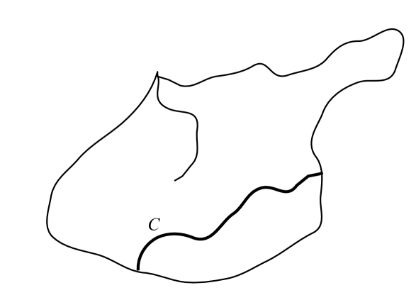
Figure 1. A crosscut

Fix an integer $N_{0}$ that is larger than the area of $D$. When $0<r_{0}<s_{0}<1$, let

$$m(s_{0},N_{0},r_{0}) = \sqrt{\frac{\pi N_{0}}{\ln(s_{0}/r_{0})}}.$$

Note that $m(s_{0},N_{0},r_{0})\rightarrow 0^{+}$ when $r_{0}\rightarrow 0^{+}$.

The central idea is to use appropriately constructed crosscuts to approximate $\phi(\zeta)$ when $|\zeta|=1$; more precisely, to treat each point on such a crosscut as an approximation of $\phi(\zeta)$. Let $C$ be such a crosscut. If $\phi(\zeta)\not\in C$, then this leads to two considerations: determining which side of $C$ the point $\phi(\zeta)$ abuts, and determining an upper bound on the diameter of this side. The crosscuts we introduce in Definition 3.1 contain enough information to resolve these issues.

Definition 3.1.

Suppose $|\zeta|=1$. Let $C$ be a crosscut of $D$. We say that $C$ recognizably bounds the value of $\phi$ on $\zeta$ if there are rational numbers $r_{0},s_{0}$ such that the following hold.

1. $0<r_{0}<s_{0}<1/2$.

2. $\phi((1-s_{0})\zeta)\in C$.

3. $C\cap A_{s_{0},\zeta}$ is connected, and $C\cap A_{s_{0},\zeta}^{+}$ has two connected components.

4. $|\phi(t\zeta)-z|>m(s_{0},N_{0},r_{0})$ whenever $z\in\overline{A_{s_{0},\zeta}^{+}\cap C}$ and $1-s_{0}\leq t\leq 1-r_{0}$.

We say that $(r_{0},s_{0})$ witnesses that $C$ recognizably bounds the value of $\phi$ on $\zeta$.

Note that it follows from Condition 3 that $C\subseteq A_{s_{0},\zeta}\cup A_{s_{0},\zeta}^{+}$. An illustration of Definition 3.1 appears in Figure 2.

Figure 2.

In Section 4, we prove the following two theorems.

Theorem 3.2.

Suppose $(r_{0},s_{0})$ witnesses that $C$ recognizably bounds the value of $\phi$ on $\zeta$. Then, $A_{r_{0},\zeta}^{+}\subseteq C^{+}$.

Thus, $\phi(\zeta)$ is a limit point of $C^{+}$.

Theorem 3.3.

Suppose $C$ recognizably bounds the value of $\phi$ on $\zeta$. If $2^{-k+1}<|\phi(0)-\phi(\zeta/2)|$, and if the diameter of $C$ is smaller than $2^{-g(k)}$, then the diameter of $C^{+}$ is at most $2^{-k+1}$.

In Section 4 we also prove the following.

Theorem 3.4.

Suppose $|\zeta|=1$. Then, there are crosscuts of arbitrarily small diameter that recognizably bound the value of $\phi$ on $\zeta$. That is, for every $\epsilon>0$ there is a crosscut that recognizably bounds the value of $\phi$ on $\zeta$ and whose diameter is smaller than $\epsilon$.

So, points on crosscuts that recognizably bound the value of $\phi$ on $\zeta$ can be used to approximate $\phi(\zeta)$ with arbitrarily small error.

3.2. Computability issues

To say that an algorithm computes with crosscuts is a chimera since there are uncountably many crosscuts but algorithms proceed by manipulating strings from a fixed finite alphabet. So, we are led to consider the approximation of crosscuts. Since a crosscut is an arc, we first discuss how we approximate arcs. Our approach is drawn from the work on computable arcs in [10] and [23]. To begin, a finite sequence of sets $(S_{1},\ldots,S_{n})$ is a chain if $S_{j}\cap S_{j+1}\neq\emptyset$ whenever $1\leq j<n$. In addition, $(S_{1},\ldots,S_{n})$ is a simple chain if $S_{j}\cap S_{k}\neq\emptyset$ only when $|j-k|=1$. We then define a wad to be a union of a chain of open rational boxes and an approximate arc to be a simple chain of wads.

When $A_{1},\ldots,A_{n}$ are subarcs of an arc $A$, we write $A=A_{1}+\ldots+A_{n}$ if $A_{j+1}$ contains exactly one point of $A_{j}$ whenever $1\leq j<n$. An approximate arc $(w_{1},\ldots,w_{n})$ approximates an arc $A$ if $A$ can be decomposed into a sum $A=A_{1}+\ldots+A_{n}$ such that $A_{j}\subseteq w_{j}$ for all $j$. Equivalently, if there are numbers $0=t_{0}<\ldots<t_{n}=1$ such that $A$ maps each number in $[t_{j-1},t_{j}]$ into $w_{j}$. The largest diameter of a wad $w_{j}$ will be referred to as the error in this approximation. In Section 5, we show that every approximate arc actually approximates an arc, and that every arc can be approximated with arbitrarily arbitrarily small error.

We define an approximate crosscut of $D$ to be an approximate arc $(w_{1},\ldots,w_{n})$ such that

• $\overline{w_{j}}\subseteq D$ when $1<j<n$, and

• $w_{j}\cap\partial D\neq\emptyset$ if $j=1,n$.

It follows from the results in Section 5 that every approximate crosscut indeed approximates a crosscut of $D$, and that every crosscut of $D$ can be approximated with arbitrarily small error by an approximate crosscut.

So, when $|\zeta|=1$, the computation of $\phi(\zeta)$ now reduces to producing approximate crosscuts that approximate, with arbitrarily small error, crosscuts of arbitrarily small diameter that recognizably bound the value of $\phi$ on $\zeta$. This leads to the following two definitions and theorem.

Definition 3.5.

Suppose that $\mathcal{C}$ is a set of crosscuts of $D$ and that $\mathcal{A}$ is a set of approximate crosscuts. We say that $\mathcal{A}$ describes $\mathcal{C}$ if the following two conditions are met.

1. Every approximate crosscut in $\mathcal{A}$ approximates a crosscut in $\mathcal{C}$.

2. Every crosscut in $\mathcal{C}$ can be approximated with arbitrarily small error by an approximate crosscut in $\mathcal{A}$. That is, if $C$ is a crosscut in $\mathcal{C}$, and if $\epsilon>0$, then $C$ is approximated by an approximate crosscut in $\mathcal{A}$ with error smaller than $\epsilon$.

We say that an algorithm enumerates a set of approximate crosscuts $\mathcal{A}$ if it has the property that whenever an approximate arc is given as input the algorithm halts if and only if the approximate arc belongs to $\mathcal{A}$.

Definition 3.6.

Let $\mathcal{C}$ be a set of crosscuts of $D$. We say that an algorithm recognizes $\mathcal{C}$ if it enumerates a set of approximate crosscuts that describes $\mathcal{C}$. We say that $\mathcal{C}$ is recognizable if at least one algorithm recognizes it.

In Section 4, we prove the following.

Theorem 3.7.

Suppose $s_{0},r_{0}$ are rational numbers and that $\zeta$ is a computable unimodular point. Let $\mathcal{C}$ be the set of all crosscuts $C$ such that $(s_{0},r_{0})$ witnesses that $C$ recognizably bounds the value of $\phi$ on $\zeta$. If $\phi$ is computable, then $\mathcal{C}$ is recognizable.

The proof of Theorem 3.7 is uniform. That is, it produces an algorithm that from $s_{0}$, $r_{0}$, an algorithm that computes $\zeta$, and an algorithm that computes $\phi$, computes an algorithm that recognizes the set of all crosscuts $C$ such that $(s_{0},r_{0})$ witnesses that $C$ recognizably bounds the value of $\phi$ on $\zeta$. This uniformity allows us to prove the following by a covering argument in Section 6.

Theorem 3.8.

If $\phi$ and $g$ are computable, then $\phi$ is strongly computable on the unit circle.

In light of Proposition 2.2, this yields the proof of the main theorem:

Theorem 3.9.

The boundary extension of a computable and conformal map of the unit disk onto a bounded domain with a computable boundary connectivity function is computable.

4. Recognizable bounding crosscuts

Our first task is to prove Theorem 3.3. We use two principles of analysis: Schwarz’s Inequality and the Lusin Area Integral. For reference, we state these theorems here. The first is stated only for the case of Lebesgue measure on $\mathbb{R}$. Schwarz’s Inequality is a consequence of Hölder’s Inequality [27]. Chapter 13 Section 1 of Greene and Krantz [12] contains a proof of Lusin’s Area Integral. Recall that when $X\subseteq\mathbb{R}^{2}$, the area of $X$ is defined to be

$$\int_{X}1\ dA$$

where $\int_{X}f\ dA$ denotes the Riemann integral of $f$ over $X$. We denote the area of $X$ by $\operatorname{Area}(X)$.

• Schwarz’s Inequality:  Let $\mu$ denote Lebesgue measure on the real line. Let $X\subseteq\mathbb{R}$ be measurable, and suppose $f,g$ are non-negative measurable functions on $X$. Then,

  $$\left(\int_{X}fg\ d\mu\right)^{2}\leq\int_{X}f^{2}d\mu\int_{X}g^{2}d\mu.$$

• Lusin Area Integral: Suppose $U$ is a domain and that $f$ is analytic and one-to-one on $U$. Then,

  $$\operatorname{Area}(f[U])=\int_{U}|f^{\prime}|^{2}dA.$$

We now set about proving Theorem 3.3. When $X_{1},X_{2}\subseteq\mathbb{C}$, let

$$d_{inf}(X_{1},X_{2})=\inf\{|z_{1}-z_{2}|\ :\ z_{1}\in X_{1}\ \wedge\ z_{2}\in X_{2}\}.$$

Lemma 4.1.

Suppose $\zeta$, $r_{0}$, $r_{1}$, $\alpha_{1}$, $\alpha_{2}$, $\Omega$ are as in Figure 3. That is:

1. $0<r_{0}<r_{1}<1$, and $|\zeta|=1$.

2. $\alpha_{1}$ and $\alpha_{2}$ are disjoint crosscuts of

   $$\{z\in\mathbb{D}\ :\ r_{0}<|z-\zeta|<r_{1}\}$$

   that do not touch the boundary of $\mathbb{D}$.

3. $\Omega$ consists of those points in the side of $\alpha_{1}$ that includes $\alpha_{2}$ that also belong to the side of $\alpha_{2}$ that includes $\alpha_{1}$.

Then,

$$\operatorname{Area}(\phi[\Omega])\geq\frac{1}{\pi}d_{inf}(\phi[\alpha_{1}],\phi[\alpha_{2}])^{2}\ln\left(\frac{r_{1}}{r_{0}}\right).$$

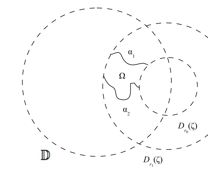
Figure 3.  

Proof.

By the Lusin Area Integral

$$\operatorname{Area}(\phi[\Omega])=\int_{\Omega}|\phi^{\prime}|^{2}dA.$$

We intend to write this integral in polar coordinates centered at $\zeta$. To this end, let $\gamma_{r}(\theta)=\zeta+r\zeta e^{i\theta}$. Note that

$$\Omega\subseteq\{\gamma_{r}(\theta)\ :\ r_{0}<r<r_{1}\ \wedge\ \frac{\pi}{2}\leq\theta\leq\frac{3\pi}{2}\}.$$

When $0<r_{0}<r<r_{1}$, let

$$S_{r}=\left\{\theta\in\left[\frac{\pi}{2},\frac{3\pi}{2}\right]:\ \gamma_{r}(\theta)\in\Omega\right\}.$$

We now change to polar coordinates and obtain

$$\int_{\Omega}|\phi^{\prime}|^{2}\ dA = \int_{r_{0}}^{r_{1}}\int_{S_{r}}|\phi^{\prime}(\gamma_{r}(\theta))|^{2}rd\theta dr$$

$$= \int_{r_{0}}^{r_{1}}\left(r\int_{S_{r}}|\phi^{\prime}(\gamma_{r}(\theta))|^{2}d\theta\right)dr$$

$$\geq \frac{1}{\pi}\int_{r_{0}}^{r_{1}}\frac{1}{r}\left(\int_{S_{r}}r^{2}d\theta\int_{S_{r}}|\phi^{\prime}(\gamma_{r}(\theta))|^{2}d\theta\right)dr.$$

By Schwarz’s Inequality,

$$\int_{S_{r}}r^{2}d\theta\ \int_{S_{r}}|\phi^{\prime}(\gamma_{r}(\theta))|^{2}d\theta\geq\left(\int_{S_{r}}r|\phi^{\prime}(\gamma_{r}(\theta))|d\theta\right)^{2}.$$

When $r_{0}<r<r_{1}$, let:

$$\theta_{r,1} = \max\left\{\theta\in\left[\frac{\pi}{2},\frac{3\pi}{2}\right]:\ \gamma_{r}(\theta)\in\alpha_{1}\right\}$$

$$\theta_{r,2} = \min\left\{\theta\in\left[\frac{\pi}{2},\frac{3\pi}{2}\right]:\ \gamma_{r}(\theta)\in\alpha_{2}\right\}$$

Then,

$$\int_{S_{r}}r|\phi^{\prime}(\gamma_{r}(\theta))|\ d\theta \geq \int_{\theta_{r,1}}^{\theta_{r,2}}r|\phi^{\prime}(\gamma_{r}(\theta))|\ d\theta$$

$$= \int_{\theta_{r,1}}^{\theta_{r,2}}\left|\frac{d}{d\theta}\phi(\gamma_{r}(\theta))\right|d\theta.$$

The latter integral is the length of the arc traced by $\phi(\gamma_{r}(\theta))$ as $\theta$ ranges from $\theta_{r,1}$ to $\theta_{r,2}$. This in turn is at least as large as the minimum distance between $\phi[\alpha_{1}]$ and $\phi[\alpha_{2}]$. Pulling all this together, we obtain

$$\operatorname{Area}(\Phi[\Omega]) \geq \frac{1}{\pi}\int_{r_{0}}^{r_{1}}\frac{1}{r}d_{inf}(\phi[\alpha_{1}],\phi[\alpha_{2}])^{2}\ dr$$

$$= \frac{1}{\pi}d_{inf}(\phi[\alpha_{1}],\phi[\alpha_{2}])^{2}\ln\left(\frac{r_{1}}{r_{0}}\right).$$

∎

When $z_{1},z_{2}\in\mathbb{C}$ are distinct, let $[z_{1},z_{2}]$ denote the line segment from $z_{1}$ to $z_{2}$.

Lemma 4.2.

Suppose $|\zeta|=1$ and $0<r_{0}<s_{0}<1$. Suppose $C$ is an arc from a point $p\in A_{s_{0},\zeta}$ to a point $q\in\partial D$ such that $C\cap\partial D=\{q\}$ and such that $|\phi(t\zeta)-z|\geq m(s_{0},N_{0},r_{0})$ whenever $1-s_{0}\leq t\leq 1-r_{0}$ and $z\in C$. Then, no point of $A_{r_{0},\zeta}^{+}$ belongs to $C$.

Proof.

By way of contradiction, suppose otherwise. Since $C\cap\partial D=\{q\}$, it follows that $\phi^{-1}[C-\{q\}]$ starts at a point $\zeta_{0}$ on the boundary of $D_{s_{0}}(\zeta)$ and crosses the boundary of $D_{r_{0}}(\zeta)$; let $\zeta_{1}$ be the first point at which it does so. Let $\alpha_{1}$ be the subarc of $\phi^{-1}[C]$ from $\zeta_{0}$ to $\zeta_{1}$. Let $\alpha_{2}=[(1-s_{0})\zeta,(1-r_{0})\zeta]$. It follows from Lemma 4.1 that

$$\operatorname{Area}(D)\geq\frac{1}{\pi}m(s_{0},N_{0},r_{0})^{2}\ln\left(\frac{s_{0}}{r_{0}}\right)\geq N_{0}>Area(D).$$

This is a contradiction and the proof is complete. ∎

of Theorem 3.2.

We first note that if $U$ is a connected subset of $D$ that contains no point of $C$, then $U$ must be included in a side of $C$. Since $r_{0}<s_{0}$, $\phi((1-r_{0})\zeta)\in C^{+}$. In addition, $\phi((1-r_{0})\zeta)$ is a boundary point of $A_{r_{0},\zeta}^{+}$. Thus, $C^{+}$ contains at least one point of $A_{r_{0},\zeta}^{+}$. Since $A_{r_{0},\zeta}^{+}$ is connected, if $A_{r_{0},\zeta}^{+}$ is not included in $C^{+}$, then it must contain a point of $C$. Let $C_{2}=C\cap A_{s_{0},\zeta}$, and let $C_{1}$ and $C_{3}$ be the connected components of $A_{s_{0},\zeta}^{+}\cap C$. Since $s_{0}<r_{0}$, $A_{r_{0},\zeta}^{+}$ contains no point of $C_{2}$. It follows from Lemma 4.2 and Definition 3.6. that $C_{1}\cup C_{2}$ contains no point of $A_{r_{0},\zeta}^{+}$. Since $A_{r_{0},\zeta}^{+}\cap C=\emptyset$, it follows that $A_{r_{0},\zeta}^{+}\subseteq C^{+}$. ∎

of Theorem 3.3.

Let $\operatorname{diam}(X)$ denote the diameter of $X$. Let $\tau$ be an arc in the boundary of $D$ that joins the endpoints of $C$. Since the diameter of $C$ is not larger than $2^{-g(k)}$, we can assume that the diameter of $\tau$ is smaller than $2^{-k}$. Let $J=C\cup\tau$. Thus, $J$ is a Jordan curve. Since $g$ is increasing, $g(x)\geq k$. Thus, the diameter of $J$ is at most $2^{-k+1}$. Note that the diameter of the interior of $J$ is identical to the diameter of $J$. Since $s_{0}<1/2$ (by Definition 3.6), $\phi(\zeta/2)\in A_{s_{0},\zeta}^{-}$. However, $A_{s_{0},\zeta}^{-}\subseteq C^{-}$ and so $\phi(\zeta/2)\in C^{-}$. On the other hand, since $2^{-k+1}<|\phi(0)-\phi(\zeta/2)|$ (by assumption), the interior of $J$ does not include $C^{-}$.

We now claim that the interior of $J$ contains a point of $D-C$. For, let $p\in C\cap D$. Thus, $p\in J$. So, $p$ is a boundary point of the interior of $J$. Since $p\in D$, $D$ includes an open disk centered at $p$. Thus, this disk contains a point in the interior of $J$; let $q$ denote such a point. Therefore $q\not\in C$ (since $C\subseteq J$) and $q\in D$.

Since $q\in D-C$, $q$ belongs to one and only one side of $C$; let $S$ denote this side. We claim that the interior of $J$ includes $S$. For, suppose $q_{1}$ is a point in $S$ besides $q$. Since $S$ is open and connected, it includes an arc $\sigma$ from $q$ to $q_{1}$. Since $S$ includes $\sigma$, $\sigma$ contains no point of $C$. Since $D$ includes $\sigma$, and since the boundary of $D$ includes $\tau$, $\sigma$ contains no point of $\tau$. Thus, $\sigma$ never crosses $J$, and so $q_{1}$ belongs to the interior of $J$. Thus, the interior of $J$ includes $S$.

It now follows that $S=C^{+}$. Since the diameter of $J$ is at most $2^{-k+1}$, the diameter of $C^{+}$ is at most $2^{-k+1}$. ∎

We now show that there are arbitrarily small crosscuts that recognizably bound the value of $\phi$ on a unimodular $\zeta$. We use the following.

Proposition 4.3.

The pre-image of $\phi$ on a finite subset of the boundary of $D$ has empty interior (in the relative topology on $\partial\mathbb{D}$).

Proof.

By way of contradiction, suppose otherwise. It follows that there is a point $\zeta$ that belongs to the boundary of $D$ and whose pre-image under $\phi$ includes an arc $G$. Let $C$ be a crosscut of the unit disk whose endpoints are the endpoints of $G$. Then, $\phi[C]\cup\{\zeta\}$ is a Jordan curve, and $\phi$ conformally maps the interior of $G\cup C$ onto the interior of $\phi[C]\cup\{\zeta\}$. It follows from the Carathéodory Theorem that the boundary extension of $\phi$ is injective. This is a contradiction since $\phi$ maps all of $G$ onto $\zeta$. ∎

Actually, much more than Proposition 4.3 is true: if $\zeta\in\partial D$, then $\phi^{-1}[\{\zeta\}]$ has measure zero. However, the pre-image of $\phi$ on a boundary point may be uncountable. See Beurling [1].

of Theorem 3.4.

Without loss of generality, we assume $\zeta=1$. The general claim then follows by applying the following argument to the map $\psi$ such that $\psi(z)=\phi(\zeta z)$ for all $z\in\mathbb{D}$. Fix a positive number $s_{0}$ that is smaller than $1/2$. Suppose $\delta>0$. It follows from Proposition 4.3 that there is a positive number $\theta_{0}$ that is smaller than $\delta$ and $\pi/2$ and such that $\phi(e^{i\theta_{0}})\neq\phi(1)$. It also follows that there is a negative number $\theta_{1}$ that is larger than $-\delta$ and $-\pi/2$ and such that $\phi(e^{i\theta_{1}})\neq\phi(1),\phi(e^{i\theta_{0}})$.

Choose $\delta$ small enough so that the lines with equations $y=\operatorname{Im}(e^{i\theta_{0}})$ and $y=\operatorname{Im}(e^{i\theta_{1}})$ cross $\partial D_{s_{0}}(1)$. Let $\sigma_{j}$ denote the intersection of the line with equation $y=\operatorname{Im}(e^{i\theta_{j}})$ with the closure of $\mathbb{D}\cap D_{s_{0}}(1)$. Let $p_{j}$ denote the endpoint of $\sigma_{j}$ on $\partial D_{s_{0}}(1)$. Let $\tau$ denote the subarc of $\partial D_{s_{0}}(1)\cap\mathbb{D}$ from $p_{1}$ to $p_{2}$. Thus, since $\phi(e^{i\theta_{0}})\neq\phi(e^{i\theta_{1}})$, the image of $\phi$ on $\sigma_{0}\cup\tau\cup\sigma_{1}$ is a crosscut of $D$. Denote this crosscut by $C$.

By allowing $s_{0}$ to approach $0$ from the right while allowing $\delta$ to approach zero from the right, we can make the diameter $C$ as small as we like. We can also choose $s_{0}$ to be rational.

Let $C_{j}=\phi[\sigma_{j}]$. Thus, $C_{0}$ and $C_{1}$ are the components of $\overline{C\cap A_{s_{0},1}^{+}}$. The key point now is that $\phi(t)\not\in C_{0}\cup C_{1}$ whenever $1-s_{0}\leq t\leq 1$. The task now is to choose $r_{0}$. We begin by letting $\delta_{1}$ denote the minimum of $|\phi(t)-z|$ as $t$ ranges from $1-s_{0}$ to $1$ and $z$ ranges over $\sigma_{0}\cup\sigma_{1}$. We can then choose $r_{0}$ so that $m(s_{0},N_{0},r_{0})<\delta_{1}$. It follows that there is a rational number $r_{0}$ between $0$ and $s_{0}$ such that $d(\phi(t),\phi[\sigma_{1}\cup\sigma_{2}])>m(s_{0},N_{0},r_{0})$ whenever $1-s_{0}\leq t\leq 1-r_{0}$. It follows that $C$, $s_{0}$, $r_{0}$ meet all conditions of Definition 3.1. ∎

5. Approximating crosscuts

Our next task is to prove Theorem 3.7. We begin with the following results on arc approximation.

Theorem 5.1.

Suppose $(w_{1},\ldots,w_{n})$ is an approximate arc and that $p,q$ are points in $w_{1},w_{n}$ respectively. Then, $(w_{1},\ldots,w_{n})$ approximates an arc from $p$ to $q$.

Proof.

Set $p_{0}=p$ and $p_{n}=q$. Choose a point $p_{j}$ in $w_{j}\cap w_{j+1}$ for each $j\in\{1,\ldots,n-1\}$. We can assume $p_{0}\neq p_{1}$ and $p_{n-1}\neq p_{n}$. Since $(w_{1},\ldots,w_{n})$ is a simple chain, it follows that $p_{0},\ldots,p_{n}$ are pairwise distinct.

Since a wad is a union of a chain of open rational rectangles, every wad is an open and connected set. So, each $w_{j}$ includes an arc from $p_{j-1}$ to $p_{j}$; call this arc $B_{j}$.

If we join the arcs $B_{1}$, $\ldots$, $B_{n}$ together we do not necessarily get an arc since, for example, $B_{2}$ may intersect $B_{1}$ at one or more points besides $p_{1}$. So, let $p_{j}^{\prime}$ be the first point on $B_{j}$ that belongs to $B_{j+1}$ for each $j\in\{1,\ldots,n-1\}$. Let $p_{0}^{\prime}=p_{0}$, and let $p_{n}^{\prime}=p_{n}$. Let $A_{j}$ be the subarc of $B_{j}$ from $p_{j-1}^{\prime}$ to $p_{j}^{\prime}$. It then follows that $A_{1}\cup\ldots\cup A_{n}$ is an arc that is approximated by $(w_{1},\ldots,w_{n})$. ∎

In the proof of our next theorem, we use the following which is Theorem 3-4 of [15].

Theorem 5.2.

If $a,b$ are two points of a connected space $S$, and if $\{U_{\alpha}\}_{\alpha\in I}$ is a family of open sets that covers $S$, then there exist $\alpha_{1},\ldots,\alpha_{n}\in I$ so that $(U_{\alpha_{1}},\ldots,U_{\alpha_{n}})$ is a simple chain such that $a\in U_{\alpha_{1}}-U_{\alpha_{2}}$ and such that $b\in U_{\alpha_{n}}-U_{\alpha_{n-1}}$.

In the following proof, we will also use the fact that the connected components of an open subset of a locally connected space are open. For example, see Theorem 3-2 of [15].

Theorem 5.3.

If $A$ is an arc from $p$ to $q$, then for every positive number $\epsilon$, there is an approximation of $A$, $(w_{1},\ldots,w_{n})$, with error smaller than $\epsilon$ so that $p\in w_{1}-\overline{w_{2}}$ and $q\in w_{n}-\overline{w_{n-1}}$.

Proof.

As a function, $A$ is uniformly continuous. It follows that there are numbers $0=t_{0}<\ldots<t_{n}=1$ so that $|A(s)-A(t)|<\epsilon/3$ whenever $s,t\in[t_{j-1},t_{j}]$. Let $A_{j}$ denote the image of $A$ on $[t_{j-1},t_{j}]$. Then, $A_{j}\cap A_{k}=\emptyset$ if $|j-k|>1$. So, when $|j-k|>1$, let $\delta_{j,k}$ denote

$$\min\{|z_{1}-z_{2}|\ :\ z_{1}\in A_{j},z_{2}\in A_{k}\}.$$

Let $\delta$ denote the minimum of all $\delta_{j,k}$.

Fix $j$ for the moment. Let $\mathcal{R}$ be the set of all open rational rectangles that contain at least one point of $A_{j}$ and whose diameter is smaller than $\epsilon/3$ and $\delta/2$. If $j\in\{2,n-1\}$, then we also require that $p,q\not\in\overline{R}$. We claim that there is a chain of rectangles in $\mathcal{R}$ that covers $A_{j}$. For, let $\mathcal{S}$ be the set of all $U$ for which there is an $R\in\mathcal{R}$ such that $U$ is a connected component of $R\cap A_{j}$. Then, each set in $\mathcal{S}$ is open (in the relative topology on $A_{j}$). Let $a,b$ be the endpoints of $A_{j}$. Let $U_{\alpha_{1}},\ldots,U_{\alpha_{m}}$ be as given by Theorem 5.2. Since $(U_{\alpha_{1}},\ldots,U_{\alpha_{m}})$ is a simple chain, its union is connected. Since $a,b$ are the endpoints of $A_{j}$ it follows that $\bigcup_{k}U_{\alpha_{k}}=A_{j}$. For each $k$, there is a rectangle $R_{k}\in\mathcal{R}$ such that $U_{\alpha_{k}}$ is a connected component of $R_{k}\cap A_{j}$. It follows that $(R_{1},\ldots,R_{m})$ is a chain that covers $A_{j}$. Set $w_{j}=\bigcup_{k}R_{k}$.

By the choice of $\delta$ and the diameters of the $R$’s, $(w_{1},\ldots,w_{n})$ is a simple chain. It follows that $(w_{1},\ldots,w_{n})$ approximates $A$. It follows from the choice of $\epsilon$ that the diameter of each $w_{j}$ is smaller than $\epsilon$. ∎

We define an arc to be computable if it is the image of a map on the unit interval that is computable and injective. We then have the following.

Lemma 5.4.

If $A$ is a computable arc, then there is an algorithm that enumerates the set of all approximations of $A$.

Proof.

Let $f$ be a computable homeomorphism of $[0,1]$ with $A$. Fix an algorithm that computes $f$.

Let $(w_{1},\ldots,w_{n})$ be an approximate arc that is given as input. We first note that $(w_{1},\ldots,w_{n})$ approximates $A$ if and only if there are rational numbers $t_{0}=0<t_{1}<\ldots<t_{k}=1$ so that for each $j$, $f$ maps each point in $[t_{j-1},t_{j}]$ into $w_{j}$. We then note that $f$ maps an interval $[a,b]$ into an open set $U$ just in case there are open rational rectangles $R_{1}$, $\ldots$, $R_{m}$, $S_{1}$, $\ldots$, $S_{m}$ so that $[a,b]$ is covered by $\{R_{1},\ldots,R_{m}\}$, $\overline{S_{j}}\subseteq U$ for each $j$, and for each $j$ the algorithm that computes $f$ produces $S_{j}$ on input $R_{j}$. By putting these two observations together, we arrive at a search procedure that terminates if and only if $(w_{1},\ldots,w_{n})$ approximates $A$. ∎

We note that the proof of Lemma 5.4 is uniform. That is, it provides an algorithm that, given any algorithm that computes an arc $A$ as input, produces an algorithm that enumerates all approximations of $A$.

Throughout the rest of this section, let $\mathcal{C}_{(s_{0},r_{0},\zeta)}$ denote the set of all crosscuts $C$ such that $(s_{0},r_{0})$ witnesses that $C$ recognizably bounds the value of $\phi$ on $\zeta$. In order to prove Theorem 3.7, we need to define a set of approximate arcs that describes $\mathcal{C}_{(s_{0},r_{0},\zeta)}$ (see Definition 3.5). To this end, we make the following definition.

Definition 5.5.

Let $\mathcal{A}_{(s_{0},r_{0},\zeta)}$ denote the set of all approximate crosscuts of $D$ $(w_{1},\ldots,w_{n})$ for which there exist integers $j_{1}$, $j_{2}$ so that the following conditions are met.

1. $1<j_{1}<j_{2}<n$ and $0<r_{0}<s_{0}<1/2$.

2. $\{w_{j}\}_{j=j_{1}}^{j_{2}}$ approximates a subarc of $A_{s_{0},\zeta}$ that contains $\phi((1-s_{0})\zeta)$; let $L$ denote the connected component of $\phi((1-s_{0})\zeta)$ in $A_{s_{0},\zeta}\cap\bigcup_{j_{1}\leq j\leq j_{2}}w_{j}$.

3. $\overline{w_{j}}\subseteq A_{s_{0},\zeta}^{+}$ whenever $1<j<j_{1}$ and whenever $j_{2}<j<n$.

4. There is a component $E_{1}$ of $w_{j_{1}}\cap A_{s_{0},\zeta}^{+}$ such that $L\cap w_{j_{1}}\cap\partial E_{1}\neq\emptyset$ and $E_{1}\cap w_{j_{1}-1}\neq\emptyset$.

5. There is a component $E_{2}$ of $w_{j_{2}}\cap A_{s_{0},\zeta}^{+}$ such that $L\cap w_{j_{2}}\cap\partial E_{2}\neq\emptyset$ and $E_{2}\cap w_{j_{2}+1}\neq\emptyset$.

6. $|\phi(t\zeta)-z|>m(r_{0},N_{0},s_{0})$ whenever $1-s_{0}\leq t\leq 1-r_{0}$ and

   $$z\in\bigcup_{j=1}^{j_{1}}\overline{w_{j}}\cup\bigcup_{j=j_{2}}^{n}\overline{w_{j}}.$$

We now show that $\mathcal{A}_{(s_{0},r_{0},\zeta)}$ describes $\mathcal{C}_{(s_{0},r_{0},\zeta)}$. We begin with the following two lemmas.

Lemma 5.6.

Suppose $(w_{1},\ldots,w_{n})$ is an arc approximation and that $1\leq k\leq n-1$. Suppose $p_{1}\in w_{1}$, $p_{2}\in w_{k}\cap w_{k+1}$, and $p_{3}\in w_{n}$. Suppose $(w_{1},\ldots,w_{k})$ approximates an arc $A$ from $p_{1}$ to $p_{2}$ and that $(w_{k+1},\ldots,w_{n})$ approximates an arc $B$ from $p_{2}$ to $p_{3}$. Then, $(w_{1},\ldots,w_{n})$ approximates an arc $C\subseteq A\cup B$ from $p_{1}$ to $p_{2}$.

Proof.

Let $A=A_{1}+\ldots+A_{k}$ be a decomposition of $A$ with the property that $A_{j}\subseteq w_{j}$ whenever $1\leq j\leq k$. Let $B=B_{k+1}+\ldots+B_{n}$ be a decomposition of $B$ so that $B_{j}\subseteq w_{j}$ whenever $k+1\leq j\leq n$. Then, let $p_{2}^{\prime}$ be the first point on $A$ that belongs to $B$. Since $(w_{1},\ldots,w_{n})$ is a simple chain, $p_{2}^{\prime}\in w_{k}\cap w_{k+1}$. So, $p_{2}^{\prime}\not\in A_{1}\cup\ldots\cup A_{k-1}$. So, let $A_{k}^{*}$ be the subarc of $A_{k}$ from $A_{k-1}$ to $p_{2}^{\prime}$. Since $p_{2}^{\prime}\in w_{k}$, $p_{2}^{\prime}\not\in B_{k+2}\cup\ldots\cup B_{n}$. Let $B_{k+1}^{*}$ be the subarc of $B_{k+1}$ from $p_{2}^{\prime}$ to $B_{k+2}$. Let $C=A_{1}\cup\ldots\cup A_{k-1}\cup A_{k}^{*}\cup B_{k+1}^{*}\cup B_{k+2}\cup\ldots\cup B_{n}$. Then, $C$ is an arc and is approximated by $(w_{1},\dots,w_{n})$. ∎

In the following proof we use the fact that an open and connected subset of the plane is arcwise connected.

Lemma 5.7.

Suppose $(w_{1},\ldots,w_{n})\in\mathcal{A}_{(s_{0},r_{0},\zeta)}$. Let $j_{1}$, $j_{2}$, $L$, $E_{1}$, $E_{2}$ be as in Definition 5.5. Then:

1. There is an arc $G_{1}$ from a point in $E_{1}\cap w_{j_{1}-1}\cap w_{j_{1}}$ to a point $q_{1}$ in $w_{j_{1}}\cap L\cap\partial E_{1}$ so that $G_{1}\subseteq E_{1}\cup\{q_{1}\}$.

2. There is an arc $G_{2}$ from a point in $E_{2}\cap w_{j_{2}}\cap w_{j_{2}+1}$ to a point $q_{2}$ in $w_{j_{2}}\cap L\cap\partial E_{2}$ so that $G_{2}\subseteq E_{2}\cup\{q_{2}\}$.

Proof.

We first note that each boundary point of $E_{1}$ either belongs to $A_{s_{0},\zeta}$ or to the boundary of $w_{j_{1}}$. For, let $p$ be a boundary point of $E_{1}$. Suppose $p\not\in A_{s_{0},\zeta}$. Since $E_{1}\subseteq A_{s_{0},\zeta}^{+}$, $p\not\in A_{s_{0},\zeta}^{-}$. Since $(w_{1},\ldots,w_{n})$ is an approximate crosscut of $D$, $\overline{w_{j_{1}}}\subseteq D$. So, $\partial E_{1}\subseteq D$. Thus, $p\in D$ and so $p\in A_{s_{0},\zeta}^{+}$. But, $p\not\in E_{1}$ since $E_{1}$ is open. It follows that $p\not\in w_{j_{1}}$. For, if $p\in w_{j_{1}}$, then its component in $A_{s_{0},\zeta}^{+}\cap w_{j_{1}}$ is an open set that contains $p$ but no point of $E_{1}$. It now follows that $p\in\partial w_{j_{1}}$.

By Condition 4 of Definition 5.5, there is a point $q_{1}^{\prime}\in w_{j_{1}}\cap L\cap\partial E_{1}$. Let $\epsilon$ be a positive number such that $D_{\epsilon}(q_{1}^{\prime})\subseteq w_{j_{1}}$ and $D_{\epsilon}(q_{1}^{\prime})\cap A_{s_{0},\zeta}\subseteq L$. By Theorem 3-18 of [15], there is a point $q_{1}\in\partial E_{1}$ and a point $p\in E_{1}$ so that $|q_{1}-q_{1}^{\prime}|<\epsilon$ and $[p,q_{1}]\subseteq E_{1}\cup\{q_{1}\}$. Thus, $q_{1}\in L$. Let $p^{\prime}\in E_{1}\cap w_{j_{1}-1}\cap w_{j_{1}}$. Then, $E_{1}$ includes an arc from $p^{\prime}$ to $p$, $G$. Let $p^{\prime\prime}$ be the first point on $G$ that belongs to $[p,q]$. Let $G^{*}$ be the subarc of $G$ from $p^{\prime}$ to $p^{\prime\prime}$. Then, take $G_{1}=G^{*}\cup[p^{\prime\prime},q]$.

Part 2 is proved similarly. ∎

Theorem 5.8.

$\mathcal{A}_{(s_{0},r_{0},\zeta)}$ describes $\mathcal{C}_{(s_{0},r_{0},\zeta)}$.

Proof.

To begin, suppose that $(w_{1},\ldots,w_{n})$ is an approximate crosscut in $\mathcal{A}_{(s_{0},r_{0},\zeta)}$. We construct a crosscut in $\mathcal{C}_{(s_{0},r_{0},\zeta)}$ that is approximated by $(w_{1},\ldots,w_{n})$. Let $j_{1}$, $j_{2}$, and $L$ be as in the definition of $\mathcal{A}_{(s_{0},r_{0},\zeta)}$.

We first show that $(w_{1},\ldots,w_{j_{1}})$ approximates an arc $C_{1}$ such that $C_{1}\cap(A_{s_{0},\zeta}\cup\partial D)\subseteq\{C_{1}(0),C_{1}(1)\}$ and $C_{1}(1)\in L$. By Lemma 5.7, there is an arc $G\subseteq w_{j_{1}}$ from a point $p\in E_{1}\cap w_{j_{1}}\cap w_{j_{1}-1}$ to a point $q\in w_{j_{1}}\cap L$ so that $G\cap(A_{s_{0},\zeta}\cup\partial D)=\{q\}$. By Theorem 5.1, $(w_{1},\ldots,w_{j_{1}-1})$ approximates an arc $H$ from a point $p_{1}^{\prime}\in\partial D$ to $p$. Let $H=H_{1}+\ldots+H_{j_{1}-1}$ be a decomposition of $H$ so that $H_{j}\subseteq w_{j}$ for all $j$. Let $p_{1}$ be the last point on $H$ that belongs to $\partial D$. Then, $p_{1}\in w_{1}$. Since $(w_{1},\ldots,w_{n})$ is an approximate crosscut of $D$, it follows that $p_{1}\not\in H_{2}\cup\ldots\cup H_{j_{1}-1}$. Let $H_{1}^{*}$ be the subarc of $H_{1}$ from $p_{1}$ to $H_{2}$. Then, $(w_{1},\ldots,w_{j_{1}-1})$ approximates $H_{1}^{*}\cup H_{2}\cup\ldots\cup H_{j_{1}-1}$. The existence of $C_{1}$ now follows from Lemma 5.6.

We can similarly show that $\{w_{j}\}_{j=j_{2}}^{n}$ approximates an arc $C_{3}$ such that $C_{3}\cap(\partial D\cup A_{s_{0},\zeta})=\{C_{3}(0),C_{3}(1)\}$ and such that $C_{3}(0)\in L$. Let $C_{2}$ be the subarc of $A_{s_{0},\zeta}$ from $C_{1}(1)$ to $C_{3}(0)$. Then, $C:=C_{1}\cup C_{2}\cup C_{3}$ is a crosscut that is approximated by $(w_{1},\ldots,w_{n})$. Furthermore, it follows from the conditions of Definition 5.5 that $(s_{0},r_{0})$ witnesses that $C$ recognizably bounds the value of $\phi$ on $\zeta$.

Now, suppose that $C\in\mathcal{C}_{(s_{0},r_{0},\zeta)}$. Let $\epsilon>0$. We construct an approximate crosscut in $\mathcal{A}_{(s_{0},r_{0},\zeta)}$ that approximates $C$ with error less than $\epsilon$. Let $C_{1}$, $C_{3}$ denote the components of $\overline{C\cap A_{s_{0},\zeta}^{+}}$. Let $C_{2}$ denote $C\cap A_{s_{0},\zeta}$. Let $C_{2}^{\prime}$ be a subarc of $C$ from an intermediate point of $C_{1}$ to an intermediate point of $C_{3}$. Let $A_{j}$ be a subarc of $C_{j}$ that omits $C_{2}^{\prime}$ and that contains a boundary point of $D$. Let $C_{j}^{\prime}=\overline{C_{j}-(C_{2}^{\prime}\cup A_{j})}$.

Let $a_{1}$ be the endpoint of $A_{1}$ that lies on the boundary of $D$. Let $a_{2}$ be the other endpoint of $A_{1}$. Let $a_{3}$ be the other endpoint (besides $a_{2}$) of $C_{1}^{\prime}$. Let $a_{4}$ be the other endpoint of $C_{2}^{\prime}$. Let $a_{5}$ be the other endpoint of $C_{3}^{\prime}$. Let $a_{6}$ be the other endpoint of $A_{3}$, and let $a_{7}$ be the endpoint of $A_{3}$ that lies on the boundary of $D$.

We now apply Theorem 5.3. Let $(w_{2},\ldots,w_{k_{1}})$ be an approximation of $C_{1}^{\prime}$ with error smaller than $\epsilon$ so that $a_{2}\in w_{2}-\overline{w_{3}}$ and $a_{3}\in w_{k_{1}}-\overline{w_{k_{1}-1}}$. Note that $a_{2}\not\in\overline{w_{4}}\cup\ldots\cup\overline{w_{k_{1}}}$ and $a_{3}\not\in\overline{w_{2}}\cup\ldots\cup\overline{w_{k_{1}-2}}$. Let $(w_{1}^{\prime},\ldots,w_{m}^{\prime})$ be an approximation of $C_{3}^{\prime}$ with error smaller than $\epsilon$ so that $a_{4}\in w_{1}^{\prime}-\overline{w_{2}^{\prime}}$ and $a_{5}\in w_{m}^{\prime}-\overline{w_{m-1}^{\prime}}$. We can suppose $\epsilon$ is small enough so that $\overline{w_{j}}\subseteq A_{s_{0},\zeta}^{+}$ for all $j$ and $\overline{w_{j}^{\prime}}\subseteq A_{s_{0},\zeta}^{+}$ for all $j$. Fix a positive number $\delta>0$. Let $\mathcal{R}_{j}$ be a finite set of open rational rectangles so that $A_{j}\subseteq\bigcup\mathcal{R}_{j}$, $R\cap A_{j}\neq\emptyset$ for each $R\in\mathcal{R}_{j}$, and the diameter of each rectangle in $\mathcal{R}_{j}$ is smaller than $\delta$. We choose $\delta$ so that

$$\overline{\bigcup\mathcal{R}_{1}\cup\bigcup\mathcal{R}_{3}}\cap(C_{2}^{\prime}\cup\overline{\bigcup_{j}w_{2<j\leq k_{1}-1}\cup\bigcup_{1\leq j<m}w_{j}^{\prime}})=\emptyset.$$

As in the proof of Theorem 5.3, $\mathcal{R}_{j}$ contains a chain that covers $A_{j}$. Let $w_{1}=R_{1}\cup\ldots\cup R_{t}$ where $(R_{1},\ldots,R_{t})$ is a chain in $\mathcal{R}_{1}$ that covers $A_{1}$. Let $w_{m+1}^{\prime}=R_{1}^{\prime}\cup\ldots\cup R_{s}^{\prime}$ where $(R_{1}^{\prime},\ldots,R_{s}^{\prime})$ is a chain in $\mathcal{R}_{3}$ that covers $A_{3}$. So, $(w_{1},\ldots,w_{k_{1}})$ is an approximation of $A_{1}\cup C_{1}^{\prime}$ and $(w_{1}^{\prime},\ldots,w_{m+1}^{\prime})$ is an approximation of $C_{3}^{\prime}\cup A_{3}$. Let $(w_{k_{1}+1},\ldots,w_{k_{2}})$ be an approximation of $C_{2}^{\prime}$. We can choose this approximation so that the error is small enough so that $(w_{1},\ldots,w_{k_{2}},w_{1}^{\prime},\ldots,w_{m}^{\prime})$ is a simple chain. Let $w_{k_{2}+j}=w_{j}^{\prime}$ when $1\leq j\leq m+1$, and let $n=k_{2}+m+1$. It follows that $(w_{1},\ldots,w_{n})$ approximates $C$. Let $j_{1}=k_{1}+1$, and let $j_{2}=k_{2}$.

We can suppose $\epsilon$ is small enough so that if $j$ is not between $j_{1}$ and $j_{2}$, then $|\phi(t\zeta)-z|>m(s_{0},N_{0},r_{0})$ whenever $1-s_{0}\leq t\leq 1-r_{0}$ and $z\in\overline{w_{j}}$. We can also suppose $\epsilon$ is small enough so that $\overline{w_{j}}\subseteq D$ whenever $1<j\leq j_{1}$ or $j_{2}\leq j<n$. It follows that $(w_{1},\ldots,w_{n})$ belongs to $\mathcal{A}_{(s_{0}r_{0},\zeta)}$. ∎

In order to show that there is an algorithm that enumerates $\mathcal{A}_{(s_{0},r_{0},\zeta)}$ if $\zeta$ and $\phi$ are computable, we will need the following characterization of $\mathcal{A}_{(s_{0},r_{0},\zeta)}$. By a rational polygonal curve we mean a polygonal curve whose vertices are rational.

Lemma 5.9.

Suppose $(w_{1},\ldots,w_{n})$, $j_{1}$, $j_{2}$ satisfy all conditions of Definition 5.5 except possibly 4 and 5. Then, Conditions 4 and 5 are satisfied if and only if there are rational numbers $\theta_{1}$, $\theta_{1}$, open rational rectangles $R_{1}$, $R_{2}$, and rational polygonal curves $P_{1}$, $P_{2}$ such that the following hold.

1. $z_{k}:=\zeta+s_{0}\zeta e^{i\theta_{k}}\in\mathbb{D}$.

2. The subarc of $\mathbb{D}\cap\partial D_{s_{0}}(\zeta)$ from $z_{1}$ to $z_{2}$ is included in $\phi^{-1}[w_{j_{1}}\cup\ldots\cup w_{j_{2}}]$.

3. $R_{k}\subseteq\phi^{-1}[w_{j_{k}}]$ and $R_{k}\cap\partial D_{s_{0}}(\zeta)\neq\emptyset$.

4. One endpoint of $P_{1}$ is in $\phi^{-1}[w_{j_{1}-1}\cap w_{j_{1}}]$ and the other is in $R_{1}$.

5. One endpoint of $P_{2}$ is in $\phi^{-1}[w_{j_{2}+1}\cap w_{j_{2}}]$ and the other is in $R_{2}$.

6. $P_{k}\subseteq D_{s_{0}}(\zeta)\cap\phi^{-1}[w_{j_{k}}]$.

Proof.

Suppose that Conditions 1 through 6 hold. It follows from Conditions 2 and 6 of Definition 5.5 that $1-s_{0}$ is between $z_{1}$ and $z_{2}$ on $\mathbb{D}\cap\partial D_{s_{0}}(\zeta)$. Let $p_{1}$ be the endpoint of $P_{1}$ in $\phi^{-1}[w_{j_{1}-1}\cap w_{j_{1}}]$, and let $q_{1}$ be the other endpoint of $P_{1}$. Let $p_{2}$ be the endpoint of $P_{2}$ in $\phi^{-1}[w_{j_{2}+1}\cap w_{j_{2}}]$, and let $q_{2}$ be the other endpoint of $P_{2}$. Since $q_{k}\in D_{s_{0}}(\zeta)$, $[q_{k},z_{k}]\cap\partial D_{s_{0}}(\zeta)=\{z_{k}\}$. Let $G_{k}=P_{k}\cup[q_{k},z_{k}]$. Thus, $G_{k}\cap\partial D_{s_{0}}(\zeta)=\{z_{k}\}$. Hence, $\phi[G_{k}]\cap A_{s_{0},\zeta}=\{\phi(z_{k})\}$. Let $E_{k}$ be the component of $\phi(p_{k})$ in $w_{j_{k}}\cap A_{s_{0},\zeta}^{+}$. Since $P_{k}\subseteq D_{s_{0}}(\zeta)\cap\phi^{-1}[w_{j_{k}}]$, and since $R_{k}\subseteq\phi^{-1}[w_{j_{1}}]$, it follows that $\phi[G_{k}]-\{z_{k}\}\subseteq w_{j_{k}}\cap A_{s_{0},\zeta}^{+}$. Thus, $\phi(z_{k})$ is a boundary point of $E_{k}$. Since the subarc of $\mathbb{D}\cap\partial D_{s_{0}}(\zeta)$ from $z_{1}$ to $z_{2}$ is contained in $\phi^{-1}[w_{j_{1}}\cup\ldots\cup w_{j_{2}}]$, it follows that $\phi(z_{k})\in L$. Thus, Conditions 4 and 5 of Definition 5.5 hold.

Now, suppose Conditions 4 and 5 of Definition 5.5 hold. We first show that $L\cap w_{j_{k}}\cap\partial E_{k}$ contains a point of the form $\phi(\zeta+s_{0}\zeta e^{i\theta_{k}})$ where $\theta_{k}$ is a rational number. Let $q_{k}\in w_{j_{k}}\cap L\cap\partial E_{k}$. Let $\epsilon$ be a positive number such that $D_{\epsilon}(q_{k})\subseteq w_{j_{k}}$ and $D_{\epsilon}(q_{k})\cap A_{s_{0},\zeta}\subseteq L$. Let $q_{k}^{\prime}\in D_{\epsilon}(q_{k})\cap E_{k}$. Let $E_{k}^{\prime}$ be the component of $q_{k}^{\prime}$ in $D_{\epsilon}(q_{k})\cap E_{k}$. Thus, $E_{k}^{\prime}\subseteq E_{k}$. Let $\epsilon_{1}$ be a positive number such that $D_{\epsilon_{1}}(q_{k})\cap A_{s_{0},\zeta}\subseteq D_{\epsilon}(q_{k})$. By Proposition 5.2 of [22], $D_{\epsilon_{1}}(q_{k})\cap A_{s_{0},\zeta}\subseteq\partial E_{k}^{\prime}$. On the other hand, $A_{s_{0},\zeta}\cap\partial E_{k}^{\prime}\subseteq\partial E_{k}$. Choose a rational number $\theta_{k}$ so that $\phi(\zeta+s_{0}\zeta e^{i\theta_{k}})\in D_{\epsilon_{1}}(q_{k})$.

Set $z_{k}=\zeta+s_{0}\zeta e^{i\theta_{k}}$. By construction, $\phi(z_{k})\in w_{j_{k}}$. It follows from Conditions 2 and 6 of Definition 5.5 that $1-s_{0}$ is between $z_{1}$ and $z_{2}$ on $\mathbb{D}\cap\partial D_{s_{0}}(\zeta)$. Choose an open rational rectangle $R_{k}$ so that $\overline{R_{k}}\subseteq\phi^{-1}[w_{j_{k}}]$ and $z_{k}\in R_{k}$. Since $\phi(z_{k})\in\partial E_{k}$, $z_{k}\in\partial\phi^{-1}[E_{k}]$. Thus, $R_{k}$ contains a point of $\phi^{-1}[E_{k}]$. Since $R_{k}\cap\phi^{-1}[E_{k}]$ is open, it contains a rational point $r_{k}$. Since $E_{1}$ contains a point of $w_{j_{1}-1}\cap w_{j_{1}}$, $\phi^{-1}[E_{1}]$ contains a point of $\phi^{-1}[w_{j_{1}-1}\cap w_{j_{1}}]$. Since this set is open, it contains a rational point $p_{1}$. Similarly, $\phi^{-1}[E_{2}]$ contains a rational point $p_{2}$ of $\phi^{-1}[w_{j_{2}+1}\cap w_{j_{2}}]$. Since $\phi^{-1}[E_{k}]$ is open and connected, it contains a rational polygonal curve $P_{k}$ from $p_{k}$ to $r_{k}$. Hence, $P_{k}\subseteq D_{s_{0}}(\zeta)\cap\phi^{-1}[w_{j_{k}}]$. ∎

of Theorem 3.7.

Suppose $\zeta$ and $\phi$ are computable. It suffices to exhibit an algorithm that enumerates $\mathcal{A}_{(s_{0},r_{0},\zeta)}$. Let $(w_{1},\ldots,w_{n})$ be given as input. By Hertling’s Effective Riemann Mapping Theorem (see Section 2), $D$ is computably open and its boundary is computably closed. So, there is a search procedure that terminates if and only if $(w_{1},\ldots,w_{n})$ approximates a crosscut of $D$. Suppose this procedure terminates. Fix $j_{1}$ and $j_{2}$.

We then check that Condition 1 of Definition 5.5 is met. If it is, then we proceed by searching for rational numbers $q_{1},q_{2}$ so that $\frac{\pi}{2}<q_{1}<\pi<q_{2}<\frac{3\pi}{2}$ and so that $\{w_{j}\}_{j=j_{1}}^{j_{2}}$ approximates the subarc of $A_{s_{0},\zeta}$ with endpoints $\phi(\zeta+s_{0}\zeta e^{iq_{1}})$ and $\phi(\zeta+s_{0}\zeta e^{iq_{2}})$. Here, we are applying the uniform version of Lemma 5.4. This search terminates if and only if Condition 2 of Definition 5.5 is met.

Suppose this search terminates as well. It is well-known that if $f:\mathbb{D}\rightarrow\mathbb{C}$ is computable, and if $U$ is computably open, then $f^{-1}[U]$ is computably open. Furthermore, this result is uniform. It follows that $\phi^{-1}[U]$ is computably open whenever $U$ is a computably open subset of $D$. The sets $w_{j_{1}}$, $w_{j_{2}}$, $w_{j_{1}-1}\cap w_{j_{1}}$, and $w_{j_{2}}\cap w_{j_{2}+1}$ are all computably open. It then follows from Lemma 5.9 that there is a search procedure that terminates if and only if Conditions 4 and 5 hold.

Suppose this search terminates. It follows from the Effective Open Mapping Theorem (see [14]) that $A_{s_{0},\zeta}^{+}$ is computably open. Furthermore, this result is uniform. So, we next search for a finite set of rational rectangles $\mathcal{B}$ so that

$$\bigcup_{1<j<j_{1}}w_{j}\cup\bigcup_{j_{2}<j<n}w_{j}\subseteq\bigcup\mathcal{B}$$

and so that $\overline{R}\subseteq A_{s_{0},\zeta}^{+}$ whenever $R\in\mathcal{B}$. It follows that this search terminates if and only if Condition 3 of Definiton 5.5 is met. If this search is successful, then we continue by searching for an approximation $(u_{1},\ldots,u_{s})$ of the arc traced by $\phi(t\zeta)$ as $t$ ranges from $1-s_{0}$ to $1-r_{0}$ so that

$$d(\bigcup_{j}\overline{u_{j}},\bigcup_{1\leq j\leq j_{1}}\overline{w_{j}}\cup\bigcup_{j_{2}\leq j\leq n}\overline{w_{j}})>m(s_{0},N_{0},r_{0}).$$

Here, we are applying the uniform version of Lemma 5.4. It follows that this search is successful if and only if Condition 6 of Definition 5.5 is met.

If for some $j_{1}$ and $j_{2}$, all of these searches terminate, then $(w_{1},\ldots,w_{n})$ belongs to $\mathcal{A}_{(s_{0},r_{0},\zeta)}$. Conversely, if $(w_{1},\ldots,w_{n})$ belongs to $\mathcal{A}_{(s_{0},r_{0},\zeta)}$, then all of these searches must halt. ∎

6. Computability of boundary extensions

We now prove Theorem 3.8 by means of the following three lemmas. When $f$ is a continuous and complex-valued function on $[0,1]$, let

$$\parallel f\parallel_{\infty}=\max\{|f(t)|\ :\ 0\leq t\leq 1\}.$$

Lemma 6.1.

Let $G$ be a crosscut of $\mathbb{D}$. Suppose $(w_{1},\ldots,w_{n})$ approximates $\phi[G]$. Then, there is a positive number $\delta$ so that $(w_{1},\ldots,w_{n})$ approximates $\phi[H]$ whenever $H$ is a crosscut of $\mathbb{D}$ such that $\parallel G-H\parallel_{\infty}<\delta$.

Proof.

Let $C=\phi[G]$. Let $C=C_{1}+\ldots+C_{n}$ be a decomposition of $C$ so that $C_{j}\subseteq w_{j}$ for all $j$. Each $C_{j}$ is compact. So, for each $j$, there is a positive number $\epsilon_{j}$ so that $z\in w_{j}$ whenever $|z-p|<\epsilon_{j}$ for some $p\in C_{j}$.

Let $G_{j}=\phi^{-1}[C_{j}]\cap G$. (It is necessary to take the intersection with $G$ in order to deal with the possibility that one or both endpoints of $C$ has more than one pre-image.) Then, $G=G_{1}\cup\ldots\cup G_{n}$, and each $G_{n}$ is closed. By compactness, for each $j$ there is a number $\delta_{j}$ so that $|\phi(z_{1})-\phi(z_{2})|<\epsilon_{j}$ whenever $z_{2}\in G_{j}$ and $|z_{1}-z_{2}|<\delta_{j}$. Let $\delta$ be the minimum of $\delta_{1},\ldots,\delta_{n}$.

There exist $t_{0},\ldots,t_{n}$ such that $0=t_{0}<t_{1}<\ldots<t_{n-1}<t_{n}=1$ and $G_{j}=G[t_{j-1},t_{j}]$. So, $\phi(G(t))=C_{j}(t)$ if $t_{j-1}\leq t\leq t_{j}$. Suppose $\parallel H-G\parallel_{\infty}<\delta$. Let $H_{j}=H[t_{j-1},t_{j}]$. Then, $H=H_{1}+\ldots+H_{n}$. If $t_{j-1}\leq t\leq t_{j}$, then $|H(t)-G(t)|<\delta$, and so $|\phi(H(t))-C_{j}(t)|<\epsilon_{j}$. Thus, $\phi[H_{j}]\subseteq w_{j}$. In other words, $\phi[H]$ is approximated by $(w_{1},\ldots,w_{n})$. ∎

Lemma 6.2.

Suppose $|\zeta|=1$ and $(s_{0},r_{0})$ witnesses that a crosscut $C$ recognizably bounds the value of $\phi$ on $\zeta$. Suppose $C$ is approximated by $(w_{1},\ldots,w_{n})$. Then, whenever $\zeta^{\prime}$ is a unimodular point that is sufficiently close to $\zeta$, $(w_{1},\ldots,w_{n})$ approximates a crosscut $C^{\prime}$ such that $(s_{0},r_{0})$ witnesses that $C^{\prime}$ recognizably bounds the value of $\phi$ on $\zeta^{\prime}$.

Proof.

Let $C_{1}=C-\partial D$. Thus, $\phi^{-1}$ is defined at every point of $C_{1}$. Let $C^{-}$ be the closure of $\phi^{-1}[C_{1}]$. Hence, $C=\phi[C^{-}]$. Suppose $|\zeta^{\prime}|=1$. When $S$ is a subset of the plane and $\xi$ is a point in the plane, let $\xi S$ denote the set of all points of the form $\xi z$ such that $z\in S$. Thus, because of the structure of $C^{-}$, $(s_{0},r_{0})$ witnesses that $\phi[(\zeta^{\prime}/\zeta)C^{-}]$ recognizably bounds the value of $\phi$ on $\zeta^{\prime}$. If $\zeta^{\prime}$ is sufficiently close to $\zeta$, then it follows from Lemma 6.1 that $\phi[(\zeta/\zeta^{\prime})C^{-}]$ is approximated by $(w_{1},\ldots,w_{n})$. ∎

Lemma 6.3.

From $k\in\mathbb{N}$ it is possible to uniformly compute a finite set of open rational rectangles $\mathcal{R}_{k}$ that covers the unit circle and so that $|\phi(z_{1})-\phi(z_{2})|<2^{-k}$ whenever $R\in\mathcal{R}_{k}$ and $z_{1},z_{2}\in R\cap\overline{\mathbb{D}}$.

Proof.

Fix $k$. Compute a positive integer $k_{0}$ such that $2^{-(k_{0}+1)}<|\phi(0)-\phi(\zeta/2)|$ for all unimodular $\zeta$.

For each rational number $\theta$, let $\zeta_{\theta}=e^{\theta i}$. Thus, the set of all $\zeta_{\theta}$’s is dense in the unit circle.

Let $\mathcal{R}_{k}^{\prime}$ be the set of all open rational rectangles $R$ for which there exist $s_{0},r_{0},\theta\in\mathbb{Q}$ and $C\in\mathcal{C}_{s_{0},r_{0},\zeta_{\theta}}$ such that $\zeta_{\theta}\in R\subseteq D_{r_{0}}(\zeta_{\theta})$ and the diameter of $C$ is smaller than $2^{-g(k+k_{0}+2)}$. It follows from the uniformity of Theorem 3.7 that $\mathcal{R}_{k}^{\prime}$ is c.e. uniformly in $k$. It follows from Theorem 3.2 and Theorem 3.3 that if $R\in\mathcal{R}_{k}^{\prime}$, and if $z_{1},z_{2}\in R\cap\overline{\mathbb{D}}$, then $|\phi(z_{1})-\phi(z_{2})|<2^{-k}$.

We claim that $\mathcal{R}_{k}^{\prime}$ covers the unit circle. For, suppose $|\zeta|=1$. By Theorem 3.4, there is a crosscut $C$ whose diameter is smaller than $2^{-g(k+k_{0}+2)}$ and that recognizably bounds the value of $\phi$ on $\zeta$. Let $(s_{0},r_{0})$ witness that $C$ recognizably bounds the value of $\phi$ on $\zeta$. Let $(w_{1},\ldots,w_{n})$ be an approximation of $C$ so that the diameter of $\bigcup_{j}w_{j}$ is smaller than $2^{-g(k+k_{0}+2)}$. By Lemma 6.2, there is a closed rational rectangle $R\subseteq D_{r_{0}}(\zeta)$ such that $\zeta\in R$ and for all $\zeta^{\prime}\in R\cap\partial\mathbb{D}$, $(w_{1},\ldots,w_{n})$ approximates a crosscut $C^{\prime}$ such that $(s_{0},r_{0})$ witnesses that $C^{\prime}$ recognizably bounds the value of $\phi$ on $\zeta^{\prime}$. The interior of $R$ contains a point of the form $\zeta_{\theta}$ for some $\theta\in\mathbb{Q}$. Since $R$ is closed, if $\zeta_{\theta}$ is close enough to $\zeta$, then $R\subseteq D_{r_{0}}(\zeta_{\theta})$. Thus, the interior of $R$ belongs to $\mathcal{R}_{k}^{\prime}$. Hence, $\partial\mathbb{D}\subseteq\bigcup\mathcal{R}_{k}^{\prime}$.

To compute $\mathcal{R}_{k}$, we enumerate $\mathcal{R}_{k}^{\prime}$ just until the unit circle is covered. ∎

of Theorem 3.8.

Let $R$ be given as input. If $R$ contains no point of the unit circle, then do not halt. Otherwise, search for the least $k$ such that $\overline{R}\not\subseteq\bigcup\mathcal{R}_{k}$. If $k=0$, then do not halt. Suppose $k>0$. Then, $\overline{R}\subseteq\bigcup\mathcal{R}_{k-1}$. Let $R_{1},\ldots,R_{t}$ be all the rectangles in $\mathcal{R}_{k-1}$ that contain a point of $\overline{R}$. For each $j$, compute a rational point $\zeta_{j}$ in $R_{j}\cap\mathbb{D}$. Then, for each $j$, compute a rational point $q_{j}$ such that $|\phi(\zeta_{j})-q_{j}|<2^{-k}$. Thus, if $z\in R$, then

$$\phi(z)\in\bigcup_{j}D_{2^{-k+1}}(q_{j}).$$

Set:

$$m_{1} = \min_{j}\operatorname{Re}(q_{j})-2^{-k+1}$$

$$M_{1} = \max_{j}\operatorname{Re}(q_{j})+2^{-k+1}$$

$$m_{2} = \min_{j}\operatorname{Im}(q_{j})-2^{-k+1}$$

$$M_{2} = \max_{j}\operatorname{Im}(q_{j})+2^{-k+1}$$

Then,

$$\bigcup_{j}D_{2^{-k+1}}(q_{j})\subseteq(m_{1},M_{1})\times(m_{2},M_{2}).$$

So, we output $(m_{1},M_{1})\times(m_{2},M_{2})$. Thus, the Strong Correctness criterion of Definition 2.1 is satisfied.

We now verify the Convergence criterion. Suppose $z\in R\cap\partial\mathbb{D}$. Set $\delta=\max_{j}|\phi(\zeta_{j})-\phi(z)|$. Let $a=\operatorname{Re}(\phi(z))$, and let $b=\operatorname{Im}(\phi(z))$. Thus,

$$(m_{1},M_{1})\times(m_{2},M_{2})\subseteq(a-\delta-2^{-k+1},a+\delta+2^{-k+1})\times(b-\delta-2^{-k+1},b+\delta+2^{-k+1}).$$

Then, $\delta\rightarrow 0^{+}$ as $\operatorname{diam}(R)\rightarrow 0^{+}$. In addition, $k\rightarrow\infty$ as $\operatorname{diam}(R)\rightarrow 0^{+}$ (otherwise, $\phi$ is constant on a neighborhood of $z$). It follows that the Convergence criterion is satisfied. ∎

7. Conclusions and questions

The creation of an algorithm to solve a problem first requires an assessment of the information that must be provided. It is shown in [21] that there is a computable conformal map of the unit disk onto a Jordan domain whose boundary extension is incomputable. Thus, the map $\phi$ by itself does not provide sufficient information for the computation of its boundary extension. We are thus led to consider what additional information must be provided. Here, we have shown that a boundary connectivity function for $D$ provides sufficient additional information. In a forthcoming paper [20], it is shown that there is a conformal map on the unit disk that has a computable boundary extension even though its range does not have a computable boundary connectivity function. Thus, a boundary connectivity function does not provide necessary additional information for the computation of boundary extensions. That is, it provides too much information.

We might then investigate other additional parameters. Since the boundary of $D$ is compact and connected, by the Hahn-Mazurkiewicz Theorem (see Section 3-5 of [15]), the boundary of $D$ is locally connected if and only if it is the range of a continuous map on the unit interval. Such a map might seem to be a reasonable and perhaps more intuitive additional parameter than a boundary connectivity function. However, it fails to provide sufficient information. For, it is quite easy to show that there is a computable map of the unit interval onto the boundary of the aforementioned example from [21]. So, pinning down the precise amount of additional information required to compute boundary extensions is still a question for investigation.

We note that the proof of Theorem 3.9 is uniform in that it produces an algorithm that given as input an algorithm for computing a conformal map $\phi$ of the unit disk onto a bounded domain $D$, an algorithm for computing a boundary connectivity function for $D$, and a rational upper bound on the area of $D$, produces an algorithm for computing the boundary extension of $\phi$. Further uniformity in the format of Type-Two Effectivity [30] also holds.

We conclude by proposing two additional and related questions:

1. What is the complexity of computing $\phi(1)$ from $\phi$, $g$?

2. Is there a proof of Pommerenke’s Theorem in the constructive framework of Bishop?

References

- [1] Arne Beurling, Ensembles exceptionnels, Acta Math. 72 (1940), 1–13.
- [2] I. Binder, M. Braverman, and M. Yampolsky, On the computational complexity of the Riemann mapping, Archiv for Matematik 45 (2007), 221–239.
- [3] Errett Bishop and Douglas Bridges, Constructive analysis, Grundlehren der Mathematischen Wissenschaften [Fundamental Principles of Mathematical Sciences], vol. 279, Springer-Verlag, Berlin, 1985.
- [4] Vasco Brattka, Plottable real number functions and the computable graph theorem, SIAM J. Comput. 38 (2008), no. 1, 303–328.
- [5] Vasco Brattka and Klaus Weihrauch, Computability on subsets of Euclidean space. I. Closed and compact subsets, Theoret. Comput. Sci. 219 (1999), no. 1-2, 65–93, Computability and complexity in analysis (Castle Dagstuhl, 1997).
- [6] M. Braverman and S. Cook, Computing over the reals: foundations for scientific computing, Notices of the American Mathematical Society 53 (2006), no. 3, 318–329.
- [7] H. Cheng, A constructive Riemann mapping theorem, Pacific Journal Mathematics 44 (1973), 435 – 454.
- [8] S. Barry Cooper, Computability theory, Chapman & Hall/CRC, Boca Raton, FL, 2004.
- [9] P.J. Couch, B.D. Daniel, and T.H. McNicholl, Computing space-filling curves, Theory of Computing Systems 50 (2012), no. 2, 370–386.
- [10] D. Daniel and T.H. McNicholl, Effective local connectivity properties, Theory of Computing Systems 50 (2012), no. 4, 621 – 640.
- [11] J. B. Garnett and D. E. Marshall, Harmonic measure, New Mathematical Monographs, vol. 2, Cambridge University Press, Cambridge, 2005.
- [12] R. Greene and S. Krantz, Function theory of one complex variable, Graduate Studies in Mathematics, American Mathematical Society, 2002.
- [13] A. Grzegorczyk, On the definitions of computable real continuous functions, Fund. Math. 44 (1957), 61–71.
- [14] P. Hertling, An effective Riemann Mapping Theorem, Theoretical Computer Science 219 (1999), 225 – 265.
- [15] John G. Hocking and Gail S. Young, Topology, second ed., Dover Publications Inc., New York, 1988.
- [16] P. Koebe, Über eine neue Methode der Konformen Abbildung und Uniformisierung, Nachr. Kgl. Ges. Wiss. Göttingen, Math.-Phys. Kl. 1912 (1912), 844–848.
- [17] Daniel Lacombe, Extension de la notion de fonction récursive aux fonctions d’une ou plusieurs variables réelles. I, C. R. Acad. Sci. Paris 240 (1955), 2478–2480. MR 0072079 (17,225d)
- [18] by same author, Extension de la notion de fonction récursive aux fonctions d’une ou plusieurs variables réelles. II, III, C. R. Acad. Sci. Paris 241 (1955), 13–14, 151–153. MR 0072080 (17,225e)
- [19] D.E. Marshall and S. Rohde, Convergence of a variant of the zipper algorithm for conformal mapping, SIAM Journal on Numerical Analysis 45 (2007), 2577–2609.
- [20] T.H. McNicholl, Conformal maps and jagged boundaries, Submitted. Preprint available at http://arxiv.org/abs/1304.1915.
- [21] by same author, An effective Carathéodory theorem, Theory of Computing Systems 50 (2012), no. 4, 579 – 588.
- [22] by same author, Computing links and accessing arcs, Mathematical Logic Quarterly 59 (2013), no. 1 - 2, 101 – 107.
- [23] by same author, The power of backtracking and the confinement of length, Proceedings of the American Mathematical Society 141 (2013), no. 3, 1041 – 1053.
- [24] P.G. Odifreddi, Classical recursion theory. the theory of functions and sets of natural numbers, first ed., North-Holland, Amsterdam, 1989.
- [25] Ch. Pommerenke, Boundary behaviour of conformal maps, Grundlehren der Mathematischen Wissenschaften [Fundamental Principles of Mathematical Sciences], vol. 299, Springer-Verlag, Berlin, 1992.
- [26] Marian B. Pour-El and J. Ian Richards, Computability in analysis and physics, Perspectives in Mathematical Logic, Springer-Verlag, Berlin, 1989.
- [27] Walter Rudin, Real and complex analysis, third ed., McGraw-Hill Book Co., New York, 1987.
- [28] E. Specker, Nicht konstruktiv beweisbare Sätze der Analysis, Journal of Symbolic Logic 14 (1949), 145 – 158.
- [29] AM Turing, with corrections from proceedings of the london mathematical society, Series 2 (1937), no. 43, 544–546.
- [30] Klaus Weihrauch, Computable analysis, Texts in Theoretical Computer Science. An EATCS Series, Springer-Verlag, Berlin, 2000.