Generalized Parton Distributions of the Photon for Nonzero $\zeta$

Abstract

We present a calculation of the generalized parton distributions of the photon when there is non-zero momentum transfer both in the transverse and longitudinal directions. We consider only the contributions when the photon helicity is not flipped and calculate those at leading order in electromagnetic coupling $\alpha$ and zeroth order in the strong coupling $\alpha_{s}$. We keep the leading logarithmic terms as well as the quark mass terms in the vertex. By taking Fourier transforms of the GPDs with respect to the transverse and longitudinal momentum transfer, we obtain the parton distributions of the photon in position space.

I Introduction

There has been a lot of progress recently in the study of exclusive processes like deeply virtual Compton scattering (DVCS) and hard meson production. The former is the process $ep\rightarrow e\gamma p$ where there is a momentum transfer between the initial and final proton and a real photon is observed in the final state rev . At large virtuality of the inducing photon, the kinematics factorizes and the soft part can be written in terms of the generalized parton distributions (GPDs) of the proton. The GPDs are unified objects rich in content about the spatial and spin structure of the proton. In the forward limit when the momentum transfer is zero, GPDs reduce to parton distributions and their first moments give the nucleon form factors. In a similar manner, factorization for the process $\gamma^{*}(Q)\gamma\rightarrow\gamma\gamma$ was studied in pire for high $Q^{2}$ and it was shown that the amplitude can be written in terms of the GPDs of the photon in the DVCS kinematics, that is when the momentum transfer between the real photons in the initial and final states is small compared to $Q^{2}$. The same process in a different kinematical region gives information on the generalized distribution amplitudes of the photon GDA . The generalized distribution amplitudes are related to the photon GPDs by crossing. On the other hand, the parton distributions (pdfs) of the photon is of interest since a long time. They are anomalous as they show logarithmic scale dependence even at zeroth order in the QCD coupling constant $\alpha_{s}$ ph . These play an important role in photon induced high energy processes and have been studied extensively both in theory and experiments. Like the photon structure function, the photon GPDs show logarithmic scale dependence already in parton model, and are called anomalous GPDs. In pire the GPDs of the photon are identified with the Fourier transform of the matrix elements of light-front bilocal currents between photon states, and they were calculated at leading order in electromagnetic coupling $\alpha$ and zeroth order in $\alpha_{s}$ considering only leading logarithmic terms when the momentum transfer between the initial and the final photon states was purely in the longitudinal direction. In a previous work us1 , we calculated the photon GPDs when the momentum transfer was purely in the transverse direction. We expressed the photon GPDs in terms of the light-front wave functions of the target photon, which can be evaluated in perturbation theory. Fourier transform of the photon GPDs with respect to the transverse momentum transfer $\Delta^{\perp}$ gives parton distributions of the photon in the transverse position or impact parameter space. Like the proton, these have the physical interpretation of probability density burkardt . In other words, the impact parameter dependent parton distribution (pdf) $q(x,b^{\perp})$ of a photon is the probability of finding a quark with momentum fraction $x$ at a distance $b^{\perp}$ from the ’center’ of the photon in the transverse position space. Thus the photon GPDs give an interesting picture of the transverse shape of the photon in position space. When the skewness $\zeta$ is nonzero, there is also momentum transfer in the longitudinal direction. The photon GPDs obey different scale evolution equations in the regions $x>\zeta$ and $x<\zeta$ pire . In terms of overlaps of the LFWFs, these can be expressed as the overlaps of two particle wave functions in the kinematical regions $1>x>\zeta$ and $-1<x<\zeta-1$. In the region $0<x<\zeta$ there is a particle number changing overlap, similar to the proton GPDs overlap . As shown in diehl1 for the proton, when the skewness $\zeta$ is non-zero, GPDs in impact parameter space do not have a probabilistic interpretation. However, they are still interesting as they now probe the partons when the initial photon is displaced from the final photon in the transverse impact parameter space. This relative shift does not vanish when the GPDs are integrated over $x$ in the amplitude. In this work, we investigate the parton content of the photon in impact parameter space when the skewness is non-zero. We limit ourselves to the kinematical region $1>x>\zeta$ and $-1<x<\zeta-1$ where only the two-particle LFWFs contribute. As shown in us1 in our previous work, photon GPDs in impact parameter space show distinctive features compared to the proton GPDs when the momentum transfer is purely in the transverse direction. In this work we show that similar conclusion can be drawn for a more general momentum transfer which has both longitudinal and transverse components. In hadron_optics we had introduced a boost invariant longitudinal impact parameter $\sigma$ conjugate to the skewness parameter $\zeta$. It was found that the DVCS amplitude for a dressed electron target state shows diffraction pattern in $\sigma$ space. Similar pattern was observed in a simulated model for a meson and even in the holographic model for the meson. Further investigations revealed that general features of the diffraction pattern is independent of the model used for the meson or the proton GPDs and depend only on the finite upper limit of the $\zeta$ integration and the invariant momentum transfer squared $t$. However, the appearance of the diffraction pattern depend on the model of the proton GPDs manohar2 . In this work, we investigate the photon GPDs in transverse as well as longitudinal position space.

The plan of the paper is as follows : in section II we present the calculation of the photon GPDs; numerical results are given in section III. Conclusions are in section IV.

II GPDs of the photon for non-zero $\zeta$

The GPDs of the photon can be expressed as the following off-forward matrix elements defined for the real photon (target) state pire :

$$F^{q}=\int{dy^{-}\over 8\pi}e^{-iP^{+}y^{-}\over 2}\langle\gamma(P^{\prime})\mid{\bar{\psi}}(0)\gamma^{+}\psi(y^{-})\mid\gamma(P)\rangle;$$

$$\tilde{F}^{q}=\int{dy^{-}\over 8\pi}e^{-iP^{+}y^{-}\over 2}\langle\gamma(P^{\prime})\mid{\bar{\psi}}(0)\gamma^{+}\gamma^{5}\psi(y^{-})\mid\gamma(P)\rangle.$$ (1)

$F^{q}$ contributes when the photon is unpolarized and $\tilde{F}^{q}$ is the contribution from the polarized photon. We work in the light-front gauge $A^{+}=0$. The above GPDs were calculated when the momentum transferred square $t=(P-P^{\prime})^{2}$ was purely in the transverse direction in us1 , in other words, when the skewness $\zeta$ was zero. On the other hand, in pire , these were calculated when the momentum transfer was purely in the longitudinal direction or $\Delta^{\perp}=0$. We use the standard LF coordinates $P^{\pm}=P^{0}\pm P^{3},~{}y^{\pm}=y^{0}\pm y^{3}$. Since the target photon is on-shell, $P^{+}P^{-}-{P^{\perp}}^{2}=0$, the momenta of the initial and final photon are given by:

$$P = \left(\ P^{+}\ ,\ {0^{\perp}}\ ,\ 0\ \right)\ ,$$ (2)

$$P^{\prime} = \left((1-\zeta)P^{+}\ ,\ -{\Delta^{\perp}}\ ,\ {{\Delta}^{\perp 2}\over(1-\zeta)P^{+}}\right)\ ,$$ (3)

The four-momentum transfer from the target is

$$\Delta = P-P^{\prime}\ =\ \left(\zeta P^{+}\ ,\ {\Delta^{\perp}}\ ,\ {t+{\Delta^{\perp}}^{2}\over\zeta P^{+}}\right)\ ,$$ (4)

where $t=\Delta^{2}$. In addition, overall energy-momentum conservation requires $\Delta^{-}=P^{-}-P^{\prime-}$, which connects ${\Delta^{\perp}}^{2}$, $\zeta$, and $t$ according to

$$(1-\zeta)t=-{\Delta^{\perp}}^{2}.$$ (5)

The details of the method of calculating $F^{q}$ and $\tilde{F}^{q}$ using the Fock space expansion of the state was given in us1 in the limit of zero $\zeta$. Here we do the calculation when both $\zeta$ and $\Delta^{\perp}$ are non-zero. There are quark and antiquark contributions respectively for $\zeta<x<1$ and $-1<x<\zeta-1$. In this work, we restrict ourselves to these two regions. The two-particle LFWFs for the photon can be calculated in perturbation theory and are given by kundu

$$\psi_{2s_{1},s_{2}}^{\lambda}(x,q^{\perp}) = {1\over m^{2}-{m^{2}+{(q^{\perp})}^{2}\over x(1-x)}}{ee_{q}\over\sqrt{2{(2\pi)}^{3}}}\chi^{\dagger}_{s_{1}}\Big{[}{(\sigma^{\perp}\cdot q^{\perp})\over x}\sigma^{\perp}$$ (6)

$$-\sigma^{\perp}{(\sigma^{\perp}\cdot q^{\perp})\over 1-x}-i{m\over x(1-x)}\sigma^{\perp}\Big{]}\chi_{-s_{2}}\epsilon^{\perp*}_{\lambda}$$

where we have used the two-component formalism two ; kundu and $m$ is the mass of $q(\bar{q})$. $\lambda$ is the helicity of the photon and $s_{1},s_{2}$ are the helicities of the $q$ and ${\bar{q}}$ respectively. The wave functions are expressed in terms of Jacobi momenta $x_{i}={k_{i}^{+}\over P^{+}}$ and $q_{i}^{\perp}=k_{i}^{\perp}-x_{i}P^{\perp}$. These obey the relations $\sum_{i}x_{i}=1,\sum_{i}q_{i}^{\perp}=0$. The GPDs can be written in terms of the overlaps of the LFWFs as follows :

$$F^{q} = \int d^{2}q^{\perp}dx_{1}\delta(x-x_{1})\psi_{2}^{*}(\tilde{x},q^{\perp}-(1-\tilde{x})\Delta^{\perp})\psi_{2}(x_{1},q^{\perp})$$ (7)

$$~{}~{}-\int d^{2}q^{\perp}dx_{1}\delta(1+x-x_{1})\psi_{2}^{*}(\tilde{x},q^{\perp}+\tilde{x}\Delta^{\perp})\psi_{2}(x_{1},q^{\perp})$$

(a)

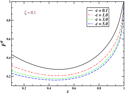
(b)

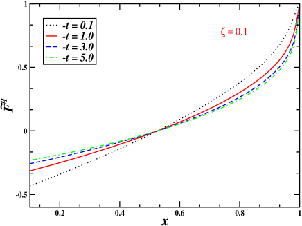
(c)

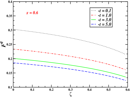
(d)

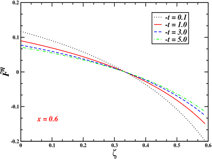
Figure 1: (Color online) (a) Plot of unpolarized GPD $F^{q}$ vs $x$ for fixed values of $-t$ in $GeV^{2}$ and at $\zeta=0.1$ and (b) polarized GPD $\tilde{F^{q}}$ vs $x$ for fixed values of $-t$ in $GeV^{2}$ and at $\zeta=0.1$ and (c) unpolarized GPD $F^{q}$ vs $\zeta$ for fixed values of $-t$ in $GeV^{2}$ and at $x=0.6$ and (d) polarized GPD $\tilde{F^{q}}$ vs $\zeta$ for fixed values of $-t$ in $GeV^{2}$ and at $x=0.6$ , $\Lambda=20\mathrm{GeV}$.

Here $\tilde{x}={x_{1}-\zeta\over 1-\zeta}$. We have suppressed the helicity indices and the sum over them. The first term is the contribution from the quarks and the second is the contribution from the antiquark in the photon. As the light-cone momentum fraction $x_{1}$ has to be always greater than zero, the first term contributes when $1>x>\zeta$ and the second term for $-1<x<\zeta-1$. We have taken $\zeta$ to be positive. There is a particle number changing overlap in the region $0<x<\zeta$, Using the LFWFs each component can be calculated separately. We calculate in the same reference frame as hadron_optics . Note that the light cone plus momentum of the target photon is non-zero. Finally we get for the unpolarized photon

(a)

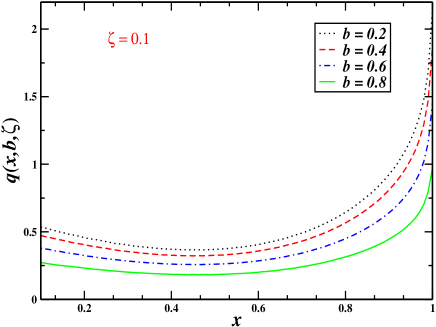
(b)

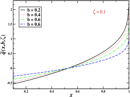
Figure 2: (Color online) (a) Plot of $q(x,\zeta,b)$ vs $x$ and (b) $\tilde{q}(x,\zeta,b)$ vs $x$ for fixed values of $b$ and at $\zeta=0.1$ (c) Plot of $q(x,\zeta,b)$ vs $b$ and (d) $\tilde{q}(x,\zeta,b)$ vs $b$ for fixed values of $x$ and at $\zeta=0.1$,where we have taken $\Lambda$ = 20 $\mathrm{GeV}$ and $\Delta_{max}$= 3GeV where $\Delta_{max}$ is the upper limit in the $\Delta$ integration. The distributions are given in $\mathrm{GeV}^{2}$ and $b$ is in ${\mathrm{GeV}}^{-1}$.

(c)

(d)

$$F^{q} = \sum_{q}{\alpha e_{q}^{2}\over 4{\pi}^{2}}\Big{[}(1-x^{\prime}-x+2x^{\prime}x)(I_{1}+I_{2}+LI_{3})+2m^{2}I_{3}\big{]}\theta(1-x)\theta(x-\zeta)$$ (8)

$$~{}~{}-\sum_{q}{\alpha e_{q}^{2}\over 4{\pi}^{2}}\Big{[}(-x-x"+2(1+x)x")(I^{\prime}_{1}+I^{\prime}_{2}+L^{\prime}I^{\prime}_{3})+2m^{2}I^{\prime}_{3}\Big{]}\theta(1+x)\theta(1+x-\zeta);$$

where $x^{\prime}={x-\zeta\over 1-\zeta}$ and $x"={1+x-\zeta\over 1-\zeta}$. Here the sum indicates sum over different quark flavors; $L=-2m^{2}+m^{2}x(1-x)+m^{2}x^{\prime}(1-x^{\prime})-{(\Delta^{\perp})}^{2}(1-x^{\prime})^{2}$, $L^{\prime}=-2m^{2}-m^{2}x(1+x)+m^{2}x"(1-x")-{(\Delta^{\perp})}^{2}x"^{2}$; the integrals can be written as,

(a)

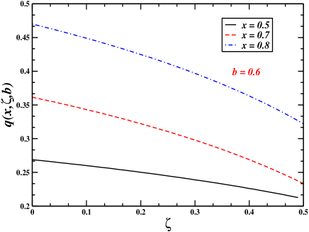
(b)

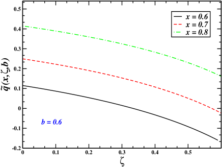
Figure 3: (Color online) (a) Plot of $q(x,\zeta,b)$ vs $\zeta$ and (b) $\tilde{q}(x,\zeta,b)$ vs $\zeta$ for fixed values of $x$ and at $b=0.6$ (c) Plot of $q(x,\zeta,b)$ vs $\zeta$ and (d) $\tilde{q}(x,\zeta,b)$ vs $\zeta$ for fixed values of $b$ and at $x=0.6$,where we have taken $\Lambda$ = 20 $\mathrm{GeV}$ and $\Delta_{max}$= 3GeV where $\Delta_{max}$ is the upper limit in the $\Delta$ integration. The distributions are given in $\mathrm{GeV}^{2}$ and $b$ is in ${\mathrm{GeV}}^{-1}$.

(c)

(d)

$$I_{1}=\int{d^{2}q^{\perp}\over D}=\pi Log\Big{[}{\Lambda^{2}\over\mu^{2}-m^{2}x(1-x)+m^{2}}\Big{]}$$

$$I_{2}=\int{d^{2}q^{\perp}\over D^{\prime}}=\pi Log\Big{[}{\Lambda^{2}\over\mu^{2}-m^{2}x^{\prime}(1-x^{\prime})+m^{2}}\Big{]}$$

$$I_{3}=\int{d^{2}q^{\perp}\over DD^{\prime}}=\int_{0}^{1}d\alpha{\pi\over P(x,\alpha,\zeta,{(\Delta^{\perp})}^{2})}$$ (9)

where $D={(q^{\perp})}^{2}-m^{2}x(1-x)+m^{2}$ and $D^{\prime}={(q^{\perp})}^{2}+{(\Delta^{\perp})}^{2}(1-x^{\prime})^{2}-2q^{\perp}\cdot\Delta^{\perp}(1-x^{\prime})-m^{2}x^{\prime}(1-x^{\prime})+m^{2}$, and $P(x,\alpha,\zeta,{(\Delta^{\perp})}^{2})=-\alpha m^{2}x(1-x)-m^{2}(1-\alpha)x^{\prime}(1-x^{\prime})+m^{2}+\alpha(1-\alpha)(1-x^{\prime})^{2}{(\Delta^{\perp})}^{2}$. As already seen in our previous paper for zero $\zeta$, at zeroth order in $\alpha_{s}$ the results are scale dependent, this scale dependence in our approach comes from the upper limit of the transverse momentum integration $\Lambda=Q$. $\mu$ is a lower cutoff on the transverse momentum, which can be taken to zero as long as the quark mass is nonzero. We included the subdominant contributions from the mass terms in the vertex.

(a)

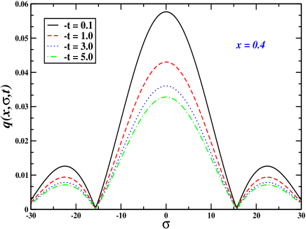
(b)

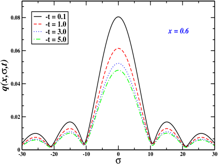
Figure 4: (Color online) (a) Plot of $q(x,\sigma,t)$ vs $\sigma$ for a fixed value of $x=0.4$ and different values of $-t$ in $GeV^{2}$, (b) same as (a) but for $x=0.6$; (c) $\tilde{q}(x,\sigma,t)$ vs $\sigma$ for a fixed value of $x=0.4$ and different values of $-t$ in $GeV^{2}$, (d) same as (c) but for $x=0.6$; we have taken $\Lambda$ = 20 $\mathrm{GeV}$.

(c)

(d)

For the antiquark contributions we have similar integrals

$$I^{\prime}_{1}=\int{d^{2}q^{\perp}\over H}=\pi Log\Big{[}{\Lambda^{2}\over\mu^{2}+m^{2}x(1+x)+m^{2}}\Big{]}$$

$$I^{\prime}_{2}=\int{d^{2}q^{\perp}\over H^{\prime}}=\pi Log\Big{[}{\Lambda^{2}\over\mu^{2}-m^{2}x"(1-x")+m^{2}}\Big{]}$$

$$I^{\prime}_{3}=\int{d^{2}q^{\perp}\over HH^{\prime}}=\int_{0}^{1}d\alpha{\pi\over Q(x,\alpha,\zeta,{(\Delta^{\perp})}^{2})}$$ (10)

where $H={(q^{\perp})}^{2}+m^{2}x(1+x)+m^{2}$ and $H^{\prime}={(q^{\perp})}^{2}+{(\Delta^{\perp})}^{2}x"^{2}+2q^{\perp}\cdot\Delta^{\perp}x"-m^{2}x"(1-x")+m^{2}$, and $Q(x,\alpha,\zeta,{(\Delta^{\perp})}^{2})=\alpha m^{2}x(1+x)-(1-\alpha)x"(1-x")m^{2}+m^{2}+\alpha(1-\alpha)x"^{2}{(\Delta^{\perp})}^{2}$.

For polarized photon the GPD $\tilde{F}^{q}$ can be calculated from the terms of the form $\epsilon^{2}_{\lambda}\epsilon^{1*}_{\lambda}-\epsilon^{1}_{\lambda}\epsilon^{2*}_{\lambda}$ pire . We consider the terms where the photon helicity is not flipped. This can be written as,

$$\tilde{F}^{q} = \sum_{q}{\alpha e_{q}^{2}\over 4{\pi}^{2}}\Big{[}(x+x^{\prime}-1)(I_{1}+I_{2}+LI_{3})+2m^{2}I_{3}\big{]}\theta(1-x)\theta(x-\zeta)$$ (11)

$$+\sum_{q}{\alpha e_{q}^{2}\over 4{\pi}^{2}}\Big{[}(-x-x")(I^{\prime}_{1}+I^{\prime}_{2}+L^{\prime}I^{\prime}_{3})+2m^{2}I^{\prime}_{3}\Big{]}\theta(1+x)\theta(1+x-\zeta)$$

In the limit $\Delta^{\perp}=0$ we get the expressions in pire and the well known splitting functions in the forward limit. Starting from the expressions of photon GPDs, we define the parton distributions of the photon in impact parameter space for nonzero $\zeta$ as,

$$q(x,\zeta,b)={1\over 4\pi^{2}}\int d^{2}\Delta^{\perp}e^{-i\Delta^{\perp}\cdot b^{\perp}}F^{q}(x,\zeta,t)$$

$$\tilde{q}(x,\zeta,b)={1\over 4\pi^{2}}\int d^{2}\Delta^{\perp}e^{-i\Delta^{\perp}\cdot b^{\perp}}\tilde{F}^{q}(x,\zeta,t).$$ (12)

Here $b=\mid b^{\perp}\mid$ is the transverse impact parameter which is a measure of the transverse distance between the struck quark and the center of momentum of the photon. In the limit of zero skewness $\zeta$ the parton distributions in impact parameter space have a probabilistic interpretation burkardt . However, in most DVCS experiments $\zeta$ is nonzero, and it is of interest to investigate the GPDs in $b^{\perp}$ space with non-zero $\zeta$. As mentioned in the introduction, the physical interpretation of the parton distributions in impact parameter space was given for the proton in diehl1 when the skewness $\zeta$ is nonzero. In this case the transverse location of the target proton is different before and after the scattering. This transverse shift depends on the skewness $\zeta$ and $b$ and the information on the transverse shift is not washed out even if the GPDs are integrated over $x$ in the DVCS amplitude. On the other hand, the boost invariant longitudinal impact parameter $\sigma$ was first introduced in hadron_optics and it was shown that DVCS amplitude shows a diffraction pattern in longitudinal impact parameter space. GPDs for the proton when expressed in term of $\sigma$ also exhibit the similar diffraction pattern manohar2 . In the same way here we introduce the boost invariant longitudinal impact parameter conjugate to the longitudinal momentum transfer as $\sigma=\frac{1}{2}b^{-}P^{+}$. The photon GPDs in longitudinal position space is given by:

$$q(x,\sigma,t)=\frac{1}{2\pi}\int_{0}^{\zeta_{max}}d\zeta e^{i\zeta P^{+}b^{-}/2}F^{q}(x,\zeta,t)=\frac{1}{2\pi}\int_{0}^{\zeta_{max}}d\zeta e^{i\zeta\sigma}F^{q}(x,\zeta,t)$$

$$\tilde{q}(x,\sigma,t)=\frac{1}{2\pi}\int_{0}^{\zeta_{max}}d\zeta e^{i\zeta P^{+}b^{-}/2}\tilde{F}^{q}(x,\zeta,t)=\frac{1}{2\pi}\int_{0}^{\zeta_{\max}}d\zeta e^{i\zeta\sigma}\tilde{F}^{q}(x,\zeta,t)$$ (13)

In the numerical calculation, we shall consider only in the region $\zeta<x<1$, and the upper limit of $\zeta$ integration $\zeta_{max}$ will be taken as $x$.

(a)

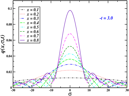
(b)

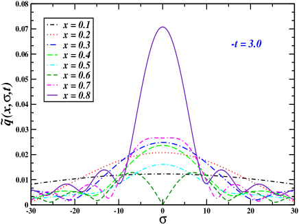
(c)

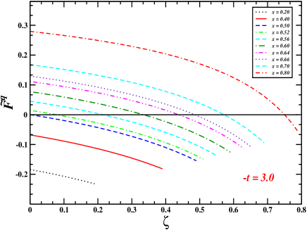
(d)

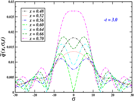
Figure 5: (Color online) Plots of (a) $q(x,\sigma,t)$ and (b) $\tilde{q}(x,\sigma,t)$ vs $\sigma$ for fixed $t$ in ${GeV}^{2}$ and different values of $x$ ; (c) $\tilde{F^{q}}$ vs $\zeta$ for $-t=3.0$ ${GeV}^{2}$ and different values of $x$ ,(d) $\tilde{q}(x,\sigma,t)$ vs $\sigma$ for fixed $t$ in ${GeV}^{2}$ and different values of $x$ for which $\tilde{q}(x,\sigma,t)$ shows two maxima with a central minima

III Numerical Results

In all plots we have taken $\Lambda$ =Q= 20 GeV and $m$=0.0033 GeV. In Figs. 1(a) and (b) we have plotted the GPDs for unpolarized photon $F^{q}$ and for polarized photon $\tilde{F}^{q}$ as functions of $x$ for a fixed value of $\zeta$ and different values of $t$. Note that in all plots $x$ is positive and $x>\zeta$ so that the contribution comes from the active quark in the photon. As seen in our previous work and also in pire when $\Delta^{\perp}$ is zero, that is when the momentum transfer is purely in the longitudinal direction, $F^{q}$ is symmetric with respect to $x=1/2$ when the momentum is shared equally among the quark and the antiquark. This is the case when the subleading terms due to the quark mass at the vertex are neglected. When $\Delta^{\perp}$ is non-zero, this symmetry is not there, the effect is more prominent at lower values of $x$. We see a similar effect when both $\zeta$ and $\Delta^{\perp}$ are non-zero. Both the GPDs $F^{q}$ and $\tilde{F}^{q}$ have been normalized as in us1 to compare with pire in the limit of zero $t$. They become independent of $t$ as $x\rightarrow 1$ because in this limit all the momentum is carried by the quark in the photon. The slope of the polarized GPD changes with increase of $-t$ and at $x\approx 0.5$ it changes sign. Figs 1(c) and 1(d) show the dependence of $F^{q}$ and $\tilde{F}^{q}$ on $\zeta$ for a fixed value of $x$ and different values of $t$. Both $F^{q}$ and $\tilde{F}^{q}$ decrease steadily with increase of $\zeta$. The rate of decrease is faster for lower values of $\mid-t\mid$. In Fig. 2 we have plotted the Fourier transform (FT) of $F^{q}$ and $\tilde{F}^{q}$ with respect to $\Delta^{\perp}$ for non-zero $\zeta$. we took the upper limit of the $\Delta^{\perp}$ integration, $\Delta_{max}$=3 GeV. Figs. 2(a)- 2(d) show the plots of the impact parameter dependent parton distributions $q(x,\zeta,b)$ and $\tilde{q}(x,\zeta,b)$ both as functions of $x$ for fixed $b$ as well as functions of $b$ for fixed $x$; for a given value of $\zeta$. As stated before in our calculation we have restricted ourselves to the kinematical region $x>\zeta$. As observed for $\zeta=0$, both $q(x,\zeta,b)$ and $\tilde{q}(x,\zeta,b)$ rise sharply as $x\rightarrow 1$ as the GPDs become independent of $t$. In Figs. 3(a)-(d) we have shown the behaviour of $q(x,\zeta,b)$ and $\tilde{q}(x,\zeta,b)$ as functions of $\zeta$ for fixed $x$ and and $b=\mid b^{\perp}\mid$ values. Both decrease steadily with increase of $\zeta$. For a given $b$, the rate of decrease with $\zeta$ increases with the increase of $x$ and for a given $x$ the rate decreases with increase of $b$. At a given $\zeta$, the distributions are broader in $b$ space for $x\approx 1/2$ when both $q$ and $\bar{q}$ carry equal momenta. As stated in the introduction, the GPDs in transverse impact parameter space for non-zero $\zeta$ probe partons inside the target photon when the initial photon is displaced from the final photon in the transverse impact parameter space. The $x$ and $\zeta$ dependence of the photon GPDs play an important role in the longitudinal position space distribution which we show in Fig 4. Fig. 4 (a) and (b) show the plot of $q(x,\sigma,t)$ vs. $\sigma$ for different values of $t$ and two different values of $x$. 4 (c) and (d) show the plots of $\tilde{q}(x,\sigma,t)$ vs. $\sigma$. $q(x,\sigma,t)$ shows prominent diffraction pattern with a central maximum and several secondary maxima separated by well-defined minima at a fixed value of $x=0.4$. The diffraction pattern is not that prominent for $\tilde{q}(x,\sigma,t)$ at the same value of $x$. Also for $q(x,\sigma,t)$ the diffraction pattern becomes less prominent at higher values of $x$ and disappears at $x\approx 0.8$. $\tilde{q}(x,\sigma,t)$ show two major peaks separated by a central minimum at $x=0.6$.

In order to further study the diffraction pattern in $\sigma$ space in Figs. 5(a) and (b) we plot $q(x,\sigma,t)$ and $\tilde{q}(x,\sigma,t)$ respectively vs $\sigma$ for a fixed value of $t$ and different values of $x$. As can been seen from the plots, the positions of the first minima for both move towards smaller values of $\sigma$ as $x$ increases. We compare this observation with the diffraction pattern shown by the proton GPDs in $\sigma$ space and by the DVCS amplitude for a dressed electron. There the positions of the first minima moved in towards smaller values of $\sigma$ with the increase of $-t$. In contrast, in the case of photon GPDs the positions of the minima are independent of $-t$. An analogy with the diffraction pattern in optics was given in hadron_optics . It was conjectured that the finite range of $\zeta$ integration acts as a slit of finite width necessary to produce the diffraction pattern. $\zeta_{max}$ for a given $t$ is determined by DVCS kinematics and is proportional to $(-t)$ for the proton target of finite mass. This $\zeta_{max}$ is analogous to the slit width in optics experiments. There the width of the central maximum is inversely proportional to the slit width, and in analogy, in DVCS the width is inversely proportional to $\zeta_{\max}$ and therefore to $-t$. However the photon is massless and as seen from Eq. (5), for a photon target $\zeta_{max}$ is $1$ in the limiting sense when ${(\Delta^{\perp})}^{2}=0$ for a given $t$. In our analysis, $\zeta_{max}=x$. So the slit width in the optics analogy is proportional to $x$ and as expected the minima move to smaller values of $\sigma$ as $x$ increases. As seen in Figs. 4(d), 5(b) and 5(d), $\tilde{q}(x,\sigma,t)$ has two maxima separated by a central minimum for those values of $x$ for which $\tilde{F}^{q}$ changes sign in the $\zeta$ range covered as seen in Fig. 5 (c). At $x=0.6$, $\tilde{F}^{q}$ changes sign almost in the middle of the $\zeta$ range covered : it is positive for half of the $\zeta$ range and negative for the other half as a result $\tilde{q}(x,\sigma,t)$ has the lowest value for the minimum at $x=0.6$. Also as seen from the figs. 5 (c) and 5 (d), the central minimum for $\tilde{q}$ is not observed when $\tilde{F}^{q}$ is either positive or negative during most of the $\zeta$ region covered. Thus the pattern in $\sigma$ space depends closely on the $x,\zeta$ dependence of the photon GPDs. The height of the maxima of both $q(x,\sigma,t)$ and $\tilde{q}(x,\sigma,t)$ decrease with increasing $-t$ for a given $x$.

IV Conclusion

In this work, we have calculated the GPDs of the photon when the momentum transfer has both transverse and longitudinal components, in other words, when both $\zeta$ and $\Delta^{\perp}$ are non-zero. We calculated both the polarized and unpolarized GPDs in terms of the light-front wave functions of the photon which, in turn, can be calculated in perturbation theory. The helicity of the photon may flip in the process. In the present work we considered only the non-helicity flip terms. We calculated them at leading order in electromagnetic coupling $\alpha$ and zeroth order in strong coupling $\alpha_{s}$. We also kept the subleading mass terms in the vertex. The GPDs depend logarithmically on the scale. However, here we studied the $x,\zeta$ and $t$ dependence at a fixed scale. By taking a Fourier transform with respect to $\Delta^{\perp}$ we expressed the GPDs in the transverse impact parameter space. As already observed for zero $\zeta$, the photon GPDs show distinctive features compared to the proton GPDs in impact parameter space. For non-zero $\zeta$ similar featured are observed. We introduced a boost invariant longitudinal impact parameter $\sigma$ conjugate to $\zeta$. Taking a FT with respect to $\zeta$ we expressed the GPDs in longitudinal position space. They show an interesting pattern similar to the diffraction pattern in optics. This was also observed for the GPDs of the proton as well as in the DVCS amplitude for a dressed electron. We presented a comparative analysis of the behaviour of the photon GPDs and that of a proton in $\sigma$ space and showed that the finite range of the $\zeta$ integration as well as the $x,\zeta$ dependence of the photon GPDs determine the pattern in the longitudinal position space. As is well known, the substructure of the photon is of relevance in high energy processes. Here we showed that the photon GPDs can provide a unique picture of the structure of the photon in 3D position space. Further investigation would involve a study of the photon GPDs when the helicity is flipped. It would be interesting to understand if the GPDs of the photon obey the general properties like polynomiality and positivity. A violation of positivity was seen in the transverse impact parameter space in us1 and that needs to be investigated further. One has to remember also that a complete picture of the GPDs in $\sigma$ space would need the contribution from the region $x<\zeta$. The analysis presented here provides a major step towards understanding these objects.

V Acknowledgments

This work is supported by BRNS grant Sanction No. 2007/37/60/BRNS/2913 dated 31.3.08, Govt. of India. We thank B. Pire for suggesting this topic and for helpful discussions.

References

- (1) For reviews on generalized parton distributions, and DVCS, see M. Diehl, Phys. Rept, 388, 41 (2003); A. V. Belitsky and A. V. Radyushkin, Phys. Rept. 418 1, (2005); K. Goeke, M. V. Polyakov, M. Vanderhaeghen, Prog. Part. Nucl. Phys. 47, 401 (2001).
- (2) S. Friot, B. Pire, L. Szymanowski, Phys. Lett. B 645 153 (2007).
- (3) M. El Beiyad, B. Pire, L. Szymanowski, S. Wallon, Phys. Rev. D 78, 034009 (2008).
- (4) T. F. Walsh and P. M. Zerwas, Phys. Lett. B 44, 95 (1974); E. Witten, Nucl. Phys. B 120, 189 (1977); A. Buras, Acta. Phys. Polon. B 37, 683 (2006).
- (5) A. Mukherjee and S. Nair, arXiv:1105.5299 [hep-ph]; arXiv:1109.6755 [hep-ph].
- (6) M. Burkardt, Int. J. Mod. Phys. A 18, 173 (2003); M. Burkardt, Phys. Rev. D 62, 071503 (2000), Erratum- ibid, D 66, 119903 (2002); J. P. Ralston and B. Pire, Phys. Rev. D 66, 111501 (2002).
- (7) S. J. Brodsky, M. Diehl, D. S. Hwang, Nucl. Phys. B 596, 99 (2001); M. Diehl, T. Feldman, R. Jakob, P. Kroll, Eur. Phys. J. C 39, 1 (2005).
- (8) M. Diehl, Eur.Phys.J. C 25 (2002) 223.
- (9) S. J. Brodsky, D. Chakrabarti, A. Harindranath, A. Mukherjee and J. P. Vary, Phys. Lett. B 641, 440 (2006); Phys. Rev. D 75, 014003 (2007).
- (10) R. Manohar, A. Mukherjee, D. Chakrabarti, Phys.Rev.D83, 014004,(2011).
- (11) A. Harindranath, R. Kundu, W. M. Zhang, Phys. Rev. D 59, 094013,(1999).
- (12) W. M. Zhang, A. Harindranath, Phys. Rev. D48, 4881 (1993).
- (13) D. Chakrabarti and A. Mukherjee, Phys.Rev.D72, 034013 (2005); Phys. Rev. D71, 014038 (2005).
- (14) D. Chakrabarti, R. Manohar, A. Mukherjee, Phys. Lett. B 682, 428 (2010);