Submitted in accordance with the requirements for the degree of
Doctor of Philosophy

SCHOOL OF PHYSICS & ASTRONOMY

Classification of Entanglement in
Symmetric States

Martin Aulbach

July 2011

The candidate confirms that the work submitted is his own and that appropriate credit has been given where reference has been made to the work of others.

This copy has been supplied on the understanding that it is copyright material and that no quotation from the thesis may be published without proper acknowledgement.

List of Acronyms

LU

Local Unitary

LO

Local Operation

ILO

Invertible Local Operation

LOCC

Local Operations and Classical Communication

SLOCC

Stochastic Local Operations and Classical Communication

DC

Degeneracy Configuration

EF

Entanglement Family

GHZ

Greenberger-Horne-Zeilinger

MBQC

measurement-based quantum computation

GM

geometric measure of entanglement

LMG

Lipkin-Meshkov-Glick

MP

Majorana point

CPS

closest product state

CPP

closest product point

iff

if and only if

d.f.

degrees of freedom

List of Publications

M. Aulbach, D. Markham, and M. Murao. The maximally entangled symmetric state in terms of the geometric measure. New J. Phys. 12, 073025 (2010). eprint: arXiv:1003.5643.

(contains results presented in Chapter 2, 3 and 4)

M. Aulbach, D. Markham, and M. Murao. Geometric Entanglement of Symmetric States and the Majorana Representation. Proceedings of the 5th Conference on Theory of Quantum Computation, Communication and Cryptography, edited by W. van Dam, V. M. Kendon, and S. Severini, pp. 141–158 (LNCS, Berlin, 2010). ISBN 978-3-642-18072-9. eprint: arXiv:1010.4777.

(contains results presented in Chapter 2, 3, 4 and 6)

M. Aulbach. Symmetric entanglement classes for n qubits. in submission (2011). preprint: arXiv:1103.0271.

(contains results presented in Chapter 5)

Chapter 1 Introduction

In this preliminary chapter the subject of the present thesis is motivated and its objectives are formulated. This is followed by a brief review of some basic concepts of quantum information science, with a particular focus on entanglement theory and permutation-symmetric states, the two topics that form the main focus of this work. An overview of the subsequent chapters and the main results presented therein can be found at the end of this chapter.

1.1 Motivation

Symmetry principles hold a special place in physics, and it is easy to undervalue their significance for the historical development of many important physical theories. Newton himself did not consciously formulate his revolutionary equations of motion for any particular frame of reference, thus implicitly considering all directions and points in space to be equivalent [1]. Nearly two centuries later the symmetries of electrodynamics were encapsulated into Maxwell’s equations, taking into account both Lorentz and gauge invariance [2], but it was not before Einstein that it was realised that Maxwell’s equations are merely a consequence of the relativistic invariance, and thus symmetry, of space-time itself. In the standard model of modern particle physics the CPT-symmetry postulates that our universe is indistinguishable from one with inverted particle charges $C:q\mapsto-q$ (C-symmetry), parity inversion $P:\bm{r}\mapsto-\bm{r}$ (P-symmetry) as well as time reversal $T:t\mapsto-t$ (T-symmetry). And going beyond the standard model, the theory of supersymmetry postulates a further physical symmetry between bosons and fermions, thus leading to the postulation of yet-to-be-observed superpartners of the existing elementary particles.

Noether’s theorem outlines how continuous symmetries of physical systems give rise to conserved quantities. For example, the conservation of energy arises from translations in time, and the conversation of linear and angular momentum arises from translations and rotations in space, respectively. In quantum mechanics the corresponding conservation laws follow directly from the kinematics of the underlying theory, with physical quantities such as position and momentum being expressed by operators on vectors of a Hilbert space [1]. Many other important consequences of symmetry can be observed in quantum mechanics: The selection rules governing atomic spectra are the consequence of rotational symmetry, the different aggregation behaviour of bosons and fermions is due to the invariance or sign-change of the wave function under exchange of identical particles, and in relativistic quantum mechanics the representations of the full symmetry group – the Poincaré group – allows for a complete classification of the elementary particles [2].

The ground state of a quantum mechanical system with a finite number of degrees of freedom is symmetric [2], i.e. the state remains invariant under permutations of the system’s parts, and no part is in any way different from any other. This is a first indication that symmetric quantum states play a particular role in quantum physics. Recently it has become possible to implement certain symmetric states [3, 4, 5] or even arbitrary symmetric states [6] actively in experiments, so it is only natural to gauge their possible applications in various areas of physics. In this thesis the permutation-symmetric quantum states will be investigated from the perspective of quantum information theory [7], a young, vibrant and highly interdisciplinary research field that combines aspects of physics, mathematics, computer science, chemistry and recently even biology [8, 9]. The realisation that information is physical has lead to a revision of our understanding of how nature works, and it has given rise to a multitude of fascinating new applications. The most famous among these is probably the quantum computer, initially suggested by Feynman for efficient simulations of quantum systems [10]. Since then theorists have unearthed several intriguing algorithms where a computer operating with qubits (quantum mechanical spin-$\tfrac{1}{2}$ systems) rather than ordinary bits would provide an exponential speedup (such as Shor’s algorithm for factorisation [11]), or at least a quadratic speedup (Grover’s algorithm for database searches [12]). Other exciting applications of quantum information are the teleportation of quantum states over large distances via quantum teleportation [13], and in principle unconditionally secure communication between remote parties via quantum cryptography [14, 15]. While the experimental realisation of quantum computation and teleportation is still in its infancy, the technically more mature status of quantum cryptography has allowed the first commercial enterprises (e.g. ID Quantique) to enter the market.

Along with the superposition principle, the non-local property of entanglement is considered to be one of the most striking consequences of quantum physics. Entanglement describes quantum correlations between separate parts of a system that cannot be explained in terms of classical physics, and these correlations are of particular importance in quantum information science. Entanglement is an essential ingredient for quantum teleportation [13], superdense coding [16], measurement-based quantum computation (MBQC) [17] and some quantum cryptography protocols [15]. It can therefore be considered as a “standard currency” in many applications, and it is desirable to know which states of a given Hilbert space are the most entangled ones. Unfortunately, for systems consisting of more than two parts the quantification of entanglement is difficult due to the existence of different types of entanglement, each of which may capture a different desirable quality of a state as a resource [18]. It is therefore unsurprising that many different entanglement measures have been proposed in order to quantify the amount of entanglement of multipartite quantum states [19]. Some entanglement measures are not useful for the analysis of larger systems, due to their bipartite definition, and most measures are notoriously difficult to compute. For these reasons the present thesis focuses on the geometric measure of entanglement (GM) [20, 21], an inherently multipartite entanglement measure that is not too difficult to compute.

Returning to the concept of symmetry in physics, we recall that permutation-symmetric quantum states appear naturally in some systems [22, 23], that it is possible to prepare them experimentally [3, 4, 5, 6], and that they have found some applications [24, 25, 26, 27]. Many canonical states that appear in quantum information science are symmetric, e.g. Bell diagonal states, Greenberger-Horne-Zeilinger (GHZ) states [28], W and Dicke states [29], and the Smolin state [30]. These aspects make it worthwhile to investigate the theoretical properties as well as the practical usefulness of symmetric states for specific quantum information tasks. In particular, not much is known so far about how to categorise the entanglement present in symmetric states, and which symmetric states exhibit a high degree of entanglement. New operational implications (in terms of usefulness for certain tasks) or visualisations of symmetric states and their entanglement would also be highly desirable. With this we formulate the following goals for the thesis:

• How can the entanglement of symmetric states be classified?

• Which symmetric states are maximally entangled?

• What operational meaning do symmetric states (or their entanglement) have?

• How can symmetric states (or their entanglement) be visualised?

• What kind of links exist between symmetric states and other fields of physics and mathematics?

A central tool for our analysis of symmetric entanglement will be the Majorana representation [31], a generalisation of the Bloch sphere representation of single qubits. This will not only provide us with a very useful visual representation of symmetric states, but also allows us to classify the different types of entanglement present in symmetric states, and to simplify the search for maximal entanglement. The Majorana representation will be introduced, along with other elementary concepts of quantum information theory, during the remainder of this introductory chapter.

1.2 Quantum entanglement

In this section we will review some elementary concepts from the theory of quantum entanglement and quantum information. This is by no means a comprehensive overview, but rather a selection of those aspects that will be of particular importance in this thesis. For a comprehensive and recent review of quantum entanglement it is suggested to consult the review article composed by the Horodecki family [19].

1.2.1 Qubit and Bloch sphere

In analogy to the bit from classical information theory the smallest unit of information in quantum information theory is called the qubit, an abbreviation of “quantum bit”. In contrast to the classical bit which either takes the value $0$ or $1$, a qubit can be in any superposition of the two basis vectors $\ket{0}$ and $\ket{1}$, known as the computational basis. Physically a qubit can be realised by any quantum 2-level system, such as the spin of an electron or the polarisation of a photon. The state of a pure qubit system can be written as $\ket{\phi}=a\ket{0}+b\ket{1}$, with complex coefficients $a$ and $b$ that satisfy the normalisation condition $\lvert a\rvert^{2}+\lvert b\rvert^{2}=1$. By means of an unphysical global phase the complex phase of the first coefficient can be eliminated without restricting generality, which allows one to employ the notation $\ket{\phi}=\cos\tfrac{\theta}{2}\ket{0}+\text{e}^{\text{i}\varphi}\sin\tfrac{\theta}{2}\ket{1}$ with two real parameters $\theta\in[0,\pi]$ and $\varphi\in[0,2\pi)$. Because of the frequent use of this notation throughout the thesis, the trigonometric expressions will be abbreviated as $\text{c}_{\theta}:=\cos\tfrac{\theta}{2}$ and $\text{s}_{\theta}:=\sin\tfrac{\theta}{2}$. The famous Bloch sphere representation [7] employs this parameterisation to uniquely identify any pure qubit state with a unit vector in $\mathbb{R}^{3}$, as shown in Figure 1.1. In this picture the two basis vectors $\ket{0}$ and $\ket{1}$, which correspond to the possible values of a classical bit, are represented by the north pole and south pole of the Bloch sphere, respectively. Any other point on the surface of the sphere represents a state $\ket{\phi}=\text{c}_{\theta}\ket{0}+\text{e}^{\text{i}\varphi}\text{s}_{\theta}\ket{1}$ that is in a superposition of the two basis states $\ket{0}$ and $\ket{1}$. The measurement of such a state in the computational basis $\{\ket{0},\ket{1}\}$ yields the outcome $\ket{0}$ with probability $\lvert\text{c}_{\theta}\rvert^{2}$ and the outcome $\ket{1}$ with probability $\lvert\text{s}_{\theta}\rvert^{2}$. The natural metric on the Bloch sphere is given by the Fubini-Study metric [32], and the distance between two normalised qubits, $\ket{\phi_{1}}$ and $\ket{\phi_{2}}$, in this metric is $\gamma(\phi_{1},\phi_{2})=\arccos\lvert\braket{\phi_{1}}{\phi_{2}}\rvert$, i.e. the geometrical angle between the two corresponding points on the Bloch sphere.

\begin{overpic}[scale={.5}]{figure1_1} \put(14.0,74.0){$\ket{\phi}$} \put(44.0,61.0){$\theta$} \put(33.0,46.5){{\footnotesize$\varphi$}} \end{overpic}

Figure 1.1: Every pure state of a single qubit $\ket{\phi}=\text{c}_{\theta}\ket{0}+\text{e}^{\text{i}\varphi}\text{s}_{\theta}\ket{1}$ can be parameterised by two angles, the inclination $\theta\in[0,\pi]$ and the azimuth $\varphi\in[0,2\pi)$. They give rise to the Bloch sphere representation on the surface of a unit sphere, with the Cartesian coordinates given by $(\sin\theta\cos\varphi,\sin\theta\sin\varphi,\cos\theta)$.

Pure qubit states are mathematically expressed as vectors of the two-dimensional Hilbert space $\mathcal{H}=\mathbb{C}^{2}$, but they are unique only up to normalisation and an unphysical global phase, which results in the two real degrees of freedom that manifest themselves as the surface of the Bloch sphere. If only partial information is known about a quantum state, it has to be treated as a mixed state. While pure qubit states correspond to points on the surface of the Bloch sphere, mixed qubit states correspond to the interior of the sphere by means of the Pauli matrix representation of the density matrix

$$\rho=\frac{1}{2}(\mathbbm{1}+x\sigma_{x}+y\sigma_{y}+z\sigma_{z})=\frac{1}{2}(\mathbbm{1}+\bm{r}\bm{\sigma})\enspace,$$ (1.1)

with $\lvert\bm{r}\rvert^{2}=\lvert x\rvert^{2}+\lvert y\rvert^{2}+\lvert z\rvert^{2}\leq 1$, and where $\bm{r}=(x,y,z)\in\mathbb{R}^{3}$ is the corresponding Bloch vector within the unit sphere. The more mixed a state is, the closer it lies to the centre of the Bloch sphere, with the maximally mixed state $\rho=\mathbbm{1}$ lying at the origin of the sphere. The Pauli matrices $\sigma_{x}$, $\sigma_{y}$ and $\sigma_{z}$ give rise to the rotation operators which rotate Bloch vectors around the $X$-, $Y$- or $Z$-axis by an angle $\vartheta$:

$$\operatorname{R_{x}}(\vartheta) =\text{e}^{-\text{i}\frac{\vartheta}{2}\sigma_{x}}=\begin{pmatrix}\phantom{-}\cos\tfrac{\vartheta}{2}&-\text{i}\sin\tfrac{\vartheta}{2}\vspace*{0.5mm}\\ -\text{i}\sin\tfrac{\vartheta}{2}&\phantom{-}\cos\tfrac{\vartheta}{2}\end{pmatrix}\enspace,$$ (1.2a)

$$\operatorname{R_{y}}(\vartheta) =\text{e}^{-\text{i}\frac{\vartheta}{2}\sigma_{y}}=\begin{pmatrix}\cos\tfrac{\vartheta}{2}&-\sin\tfrac{\vartheta}{2}\vspace*{0.5mm}\\ \sin\tfrac{\vartheta}{2}&\phantom{-}\cos\tfrac{\vartheta}{2}\end{pmatrix}\enspace,$$ (1.2b)

$$\operatorname{R_{z}}(\vartheta) =\text{e}^{-\text{i}\frac{\vartheta}{2}\sigma_{z}}=\begin{pmatrix}\text{e}^{-\text{i}\frac{\vartheta}{2}}&0\\ 0&\text{e}^{\text{i}\frac{\vartheta}{2}}\end{pmatrix}\enspace.$$ (1.2c)

A rotation around an arbitrary axis $\bm{n}=(n_{x},n_{y},n_{z})$, with $\lvert\bm{n}\rvert=1$, that runs though the origin of the Bloch sphere is given by $\operatorname{R}_{\bm{n}}(\vartheta)=\text{e}^{-\text{i}\frac{\vartheta}{2}\bm{n}\bm{\sigma}}$ and can be straightforwardly calculated with the equations above. In mathematical terms the unitary operations are elements of $\text{SU}(2)$, and in general they do not keep the coefficient of the $\ket{0}$ vector of a pure state real and non-negative, so a multiplication with a suitable global phase may be necessary after rotation in order to return to the standard qubit notation $\ket{\phi}=\text{c}_{\theta}\ket{0}+\text{e}^{\text{i}\varphi}\text{s}_{\theta}\ket{1}$. For $Z$-axis rotations $\operatorname{R_{z}}(\vartheta)$ this global phase is simply $\text{e}^{\text{i}\frac{\vartheta}{2}}$, independent of the Bloch vector $\ket{\phi}$ that is being rotated.

While measurements destroy the state of an unknown qubit, this is not the case with the rotation operators described above. Applying such a unitary operation on an unknown qubit in the laboratory has the effect of a rotation of its Bloch vector around an axis on the Bloch sphere, without measuring or destroying the state unknown to the experimenter.

1.2.2 Bipartite and multipartite systems

Quantum systems that consist of two subsystems (e.g. two qubits) are commonly known as bipartite systems, while systems with three or more subsystems are referred to as multipartite systems. This seemingly arbitrary distinction will become more meaningful later when considering the qualitatively different manifestations of entanglement in bipartite and multipartite systems. Coined by Einstein as spukhafte Fernwirkung (“spooky action at a distance”), entanglement describes an inherently nonlocal correlation between detached quantum systems that is predicted by quantum theory, and which cannot be adequately described or explained in the language of classical physics, at least without making assumptions about hidden variables [35]. The nonexistence of such hidden variables in nature has been sufficiently validated experimentally over the last few decades [36], thanks to the ingenious Bell inequalities [37].

In the language of quantum mechanics, an entangled quantum system is one whose state vector cannot be expressed as the tensor product of vectors of its subsystems. In the simplest case of a bipartite quantum system this is the case if $\ket{\psi}\neq\ket{\phi_{1}}\otimes\ket{\phi_{2}}$, i.e. no description of one part is complete without information about the other. One example for two qubits is the Bell state $\ket{\psi^{+}}=\frac{1}{\sqrt{2}}\big{(}\ket{0}_{1}\ket{0}_{2}+\ket{1}_{1}\ket{1}_{2}\big{)}$ where the two subsystems are perfectly correlated with each other in the sense that the measurement of one part of the system in a suitably chosen measurement basis (for $\ket{\psi^{+}}$ the computational basis $\{\ket{0},\ket{1}\}$) mediates a “collapse” of the other part into the same state. For example, if a measurement of part $1$ in the computational basis yields $\ket{0}_{1}$, then part 2 collapses to $\ket{0}_{2}$, so any subsequent measurement of part 2 yields $\ket{0}_{2}$. In other words, the measurement turns the initially entangled state into one of the two product states $\ket{\psi_{1}}=\ket{0}_{1}\ket{0}_{2}$ or $\ket{\psi_{2}}=\ket{1}_{1}\ket{1}_{2}$ with equal probability. The most striking aspect of this is that the measurement of one part instantaneously affects the other part, regardless of the spatial distance between the subsystems. This cannot be used for superluminal communication, however, because the randomness of the measurement outcomes prevents the transmission of information by quantum measurements alone, thus preserving a central tenet of special relativity.

The Hilbert space of a multipartite system is given by the tensor product of the subsystems’ Hilbert spaces, i.e. $\mathcal{H}=\mathcal{H}_{1}\otimes\cdots\otimes\mathcal{H}_{N}$, where $\mathcal{H}_{i}$ is the Hilbert space of the $i$-th subsystem. Since quantum states are uniquely described only up to normalisation and a global phase, it makes sense to introduce the projective Hilbert space P$\mathcal{H}$ as the set of all unique pure quantum states. The standard metric on P$\mathcal{H}$ is the Fubini-Study metric [38].

A multipartite pure quantum state $\ket{\psi}\in\mathcal{H}$ is separable if and only if (iff) it can be written as a tensor product of states from the individual subsystems:

$$\ket{\psi}=\ket{\phi_{1}}\otimes\cdots\otimes\ket{\phi_{N}}\enspace,\quad\text{with}\quad\ket{\phi_{i}}\in\mathcal{H}_{i}\,\,\forall\,i\enspace.$$ (1.3)

States that are not separable are entangled. For mixed quantum states $\rho\in S(\mathcal{H})$ of a multipartite system separability is defined by the existence of a (non-unique) convex sum of product states

$$\rho=\sum_{j}p_{j}\,\rho_{1}^{j}\otimes\cdots\otimes\rho_{N}^{j}\enspace,\quad\text{with}\quad\rho_{i}^{j}\in S(\mathcal{H}_{i})\,\,\forall\,i,j\enspace.$$ (1.4)

For finite-dimensional subsystems an orthonormalised basis $\{\ket{0},\ldots,\ket{d_{i}-1}\}_{i}$ can be chosen for each subsystem, with $d_{i}$ denoting the dimension of $\mathcal{H}_{i}$. A pure quantum state of the composite system can then be cast as

$$\ket{\psi}=\sum_{i_{1}=0}^{d_{1}-1}\cdots\sum_{i_{n}=0}^{d_{n}-1}a_{i_{1},\ldots,i_{n}}\ket{i_{1}}_{1}\otimes\cdots\otimes\ket{i_{n}}_{n}\enspace,$$ (1.5)

where the $a_{i_{1},\ldots,i_{n}}$ are complex coefficients, and ${}_{j}\braket{i_{A}}{i_{B}}_{j}=\delta_{AB}$ for all $j\in\{1,\ldots,n\}$ and all $A,B\in\{0,\ldots,d_{j}-1\}$. For brevity the basis states $\ket{i_{1}}_{1}\otimes\cdots\otimes\ket{i_{n}}_{n}$ of the composite system will be abbreviated as $\ket{i_{1}}\ket{i_{2}}\cdots\ket{i_{n}}$, or simply $\ket{i_{1}i_{2}\cdots i_{n}}$. The normalisation $\braket{\psi}{\psi}=1$ will be implied throughout this thesis, except for a few cases where states are easier to represent in unnormalised form and where the normalisation does not matter.

Of particular interest in this thesis will be states whose coefficients are all real or positive. We call a quantum state $\ket{\psi}$ of the form (1.5) real if $a_{i_{1},\ldots,i_{n}}\in\mathbb{R}$ for all $i_{1},\ldots,i_{n}$, and positive if $a_{i_{1},\ldots,i_{n}}\geq 0$ for all $i_{1},\ldots,i_{n}$. It should be noted that these properties intrinsically depend on the chosen basis, and that states which are real or positive in one computational basis (a basis made up of tensors of local bases) generally do not exhibit this property in another basis. In turn, a state that is not real or positive in one basis may be recast as a real or positive state by choosing a different basis, although this is in general not possible. Only for bipartite states it is always possible to find orthonormalised bases for the subsystems so that a given state can be expressed as a positive state in the form (1.5). This is possible thanks to the Schmidt decomposition of linear algebra which – applied to quantum information – states that any pure state of a bipartite system $\ket{\psi}\in\mathcal{H}_{A}\otimes\mathcal{H}_{B}$ with $d=\min\{\dim(\mathcal{H}_{A}),\dim(\mathcal{H}_{B})\}$ can be expressed in the form

$$\ket{\psi}=\sum_{i=0}^{d-1}\alpha_{i}\ket{i}\ket{i}\enspace,\quad\text{with}\quad\alpha_{0}\geq\ldots\geq\alpha_{d-1}\geq 0\enspace,$$ (1.6)

where the non-negative numbers $\alpha_{i}$ are called the Schmidt coefficients [7]. The minimum number of nonvanishing coefficients required for the Schmidt decomposition is known as the Schmidt rank. The Schmidt decomposition and the Schmidt rank are important tools for the analysis of bipartite states, which will become clear in the next section.

Unfortunately, the elegant Schmidt decomposition (1.6) does not exist in the multipartite setting, a first indication that the bipartite case is qualitatively different from the multipartite case. Several attempts have been made to find a generalised Schmidt decomposition, a standard form for the multipartite setting which imposes certain restrictions on the coefficients of a given state by choosing suitable orthonormal bases for all subsystems [39, 40, 41, 42, 43]. Here we mention the generalised Schmidt decomposition of Carteret et al. [40] which is defined for arbitrary finite-dimensional multipartite states. For the sake of simplicity, we consider $n$ equal subsystems, each of dimension $d$. In analogy to the 2-level qubit, we refer to such a $d$-level quantum system as a qudit. The standard form imposes the following conditions on the coefficients in Equation (1.5) for the $n$ qudit case:

$$a_{\underbrace{\scriptstyle i\ldots ik\!\!}_{j\text{ indices}}i\ldots i} =0 \forall \,j,i\enspace\forall\,i<k\leq d-1\enspace,$$ (1.7a)

$$a_{\underbrace{\scriptstyle(d-1)\ldots(d-1)i}_{j\text{ indices}}(d-1)\ldots(d-1)} \geq 0 \forall \,j,i\enspace,$$ (1.7b)

$$\lvert a_{\scriptstyle ii\ldots ii}\rvert \geq\lvert a_{\scriptstyle j_{1}\ldots j_{n}}\rvert \forall \,i\enspace\forall\,i\leq j_{r}\,\,(r=1,\dots,n)\enspace.$$ (1.7c)

These conditions clearly do not necessarily result in a real or positive state in general, and most multipartite states do not allow for a real or positive representation. If the subsystems do not have equal dimensions, then the conditions are of a more complicated form. However, Equation (1.7a) straightforwardly generalises to

$$a_{\underbrace{\scriptstyle i\ldots ik\!\!}_{j\text{ indices}}i\ldots i}=0\qquad\forall\,j,i\enspace\forall\,i<k\leq d_{j}-1\enspace,$$ (1.8)

where $d_{j}$ is the dimension of subsystem $j$.

A multipartite generalisation of the Schmidt rank has also been put forward, and is commonly referred to as the tensor rank [18, 44]. This quantity is given by the minimum number of product states needed to expand a given state. The tensor rank has featured prominently in some recent works, and has been employed to find further evidence of a qualitative difference between the bipartite and multipartite setting [45].

Two well-known multipartite states with interesting entanglement features are the GHZ state [28] and the W state. In the general case of $n$ qubits their form is

$$\ket{\text{GHZ}_{n}} =\tfrac{1}{\sqrt{2}}\left(\ket{00\ldots 00}+\ket{11\ldots 11}\right)\enspace,$$ (1.9)

$$\ket{\text{W}_{n}} =\tfrac{1}{\sqrt{n}}\left(\ket{10\ldots 0}+\ket{010\ldots 0}+\ldots+\ket{00\ldots 01}\right)\enspace.$$ (1.10)

These two states have found a broad range of uses in quantum information science [19]. For example, the 3 qubit GHZ state has been employed to tell Bell’s theorem without inequalities [28], and the $n$-qubit GHZ state can be considered the most non-local with respect to all possible two-output, two-setting Bell inequalities [46]. However, the GHZ state loses all its entanglement if a particle is lost, because its one-particle reduced density matrix $\text{Tr}_{i}(\ket{\text{GHZ}_{n}}\!\bra{\text{GHZ}_{n}})=\tfrac{1}{2}(\ket{00\ldots 00}\!\bra{00\ldots 00}+\ket{11\ldots 11}\!\bra{11\ldots 11})$ is a separable state. On the other hand, W states still retain a considerable amount of entanglement after the removal of an arbitrary particle, and it has been shown that the $n$-qubit W state is the optimal state for leader election [24]. This shows that the entanglement of GHZ and W states is of a different nature, and such qualitative aspects of entanglement and their characterisation will be investigated in the next section.

1.2.3 Entanglement classes

In order to categorise different types of entanglement, it makes sense to partition the given Hilbert space into equivalence classes, with an operationally motivated definition of equivalence. The most intuitive classification scheme is that of Local Unitary (LU) equivalence. In Section 1.2.1 the effect of unitary operations on a single qubit was outlined. When generalising this concept to an arbitrary number of quantum particles distributed among spatially separated experimenters, then the local application of unitary operations on each particle is referred to as an LU operation. Such operations are both deterministic and reversible, and – from a mathematical viewpoint – equivalent to selecting a different orthonormalised basis for the computational representation of a given state. Therefore two LU-equivalent states $\rho_{\psi}\stackrel{{\scriptstyle\text{LU}}}{{\longleftrightarrow}}\rho_{\phi}$ are expected to have precisely the same physical properties, in particular the same entanglement. A comprehensive analysis of the equivalence classes of $n$ qubit pure states under LU operations has recently been achieved by Kraus [42], and subsequently employed to find the different LU equivalence classes of up to five qubits [43].

In order to perform quantum information tasks, it is necessary for the experimenters to manipulate the states of their quantum particles in more ways than by LU operations alone. The different types of quantum operations [47] that can be performed on a given state $\rho$ are the following:

• unitary transformation:                          $\rho\longmapsto U\rho U^{\dagger}\enspace,$

  where $U$ is a unitary operator.

• selective projective measurement:              $\rho\longmapsto\{p_{i},\sigma_{i}\}\enspace,$

  i.e. the measurement outcome $\sigma_{i}$ is observed with probability $p_{i}$.

• non-selective projective measurement:   $\rho\longmapsto\sum\limits_{i}p_{i}\sigma_{i}\enspace,$

  i.e. discarding the measurement outcome yields a mixture of all possible outcomes.

• addition of an ancilla system:                  $\rho\longmapsto\rho\otimes\omega\enspace,$

  where $\omega$ is an auxiliary quantum system (“ancilla”) added to the system.

• removal of a subsystem:                          $\rho\longmapsto\text{Tr}_{A}[\rho]\enspace,$

  where subsystem $A$ is removed from the quantum system by a partial trace.

These different kinds of quantum evolution can all be subsumed under linear completely positive maps $\mathcal{E}:S(\mathcal{H})\to S(\mathcal{H})$ with the help of Kraus operators [7].

As it is typically not possible in practice to perform joint operations on spatially separated particles, the quantum operations act locally. The experimenters are however able to coordinate their actions by communicating with each other over a classical channel, e.g. by telephone. This leads to the paradigm of Local Operations and Classical Communication (LOCC) whereby quantum states are modified by performing Local Operations on the subsystems and allowing the transmission of classical communication between the parties. As seen from the list of quantum operations above, such LOCC operations are in general irreversible. For the case of pure states, however, it has been shown (see Corollary 1 of [48] or Theorem 4 of [47]) that two states are LOCC-equivalent iff they are LU-equivalent. This defines a partition of the pure Hilbert space which is equivalent to the partition generated by LU equivalence. For two pure $n$ qudit states LOCC equivalence is mathematically expressed as

$$\ket{\psi}\stackrel{{\scriptstyle\text{LOCC}}}{{\longleftrightarrow}}\ket{\phi}\quad\Longleftrightarrow\quad\exists\,\mathcal{A}_{1},\ldots,\mathcal{A}_{n}\in\text{SU}(d):\ket{\psi}=\mathcal{A}_{1}\otimes\cdots\otimes\mathcal{A}_{n}\ket{\phi}\enspace,$$ (1.11)

and by definition the LOCC equivalence of two general states (denoted as $\rho_{\psi}\stackrel{{\scriptstyle\text{LOCC}}}{{\longleftrightarrow}}\rho_{\phi}$) requires that a deterministic conversion is possible in both directions. This is a much more stringent requirement than deterministic LOCC conversion in only one direction (denoted as $\rho_{\psi}\stackrel{{\scriptstyle\text{LOCC}}}{{\longmapsto}}\rho_{\phi}$). For the pure bipartite case the latter conversions are fully characterised by the theory of majorisation [49], which induces a partial order with the help of the Schmidt decomposition (1.6). More precisely, the necessary and sufficient conditions for deterministically converting a pure two-qudit state into another one are

$$\ket{\psi}\stackrel{{\scriptstyle\text{LOCC}}}{{\longmapsto}}\ket{\phi}\quad\Longleftrightarrow\quad\forall\,0\leq j\leq d-1:\sum_{i=0}^{j}\alpha_{i}^{2}\leq\sum_{i=0}^{j}{\alpha^{\prime}}_{i}^{2}\enspace,$$ (1.12)

where the $\{\alpha_{i}\}$ and $\{{\alpha^{\prime}}_{i}\}$ are the Schmidt coefficients of $\ket{\psi}$ and $\ket{\phi}$, respectively. From this is can be seen that pure bipartite states are LOCC-equivalent (or LU-equivalent) to each other iff they have the same Schmidt coefficients:

$$\ket{\psi}\stackrel{{\scriptstyle\text{LU}}}{{\longleftrightarrow}}\ket{\phi}\quad\Longleftrightarrow\quad\ket{\psi}\stackrel{{\scriptstyle\text{LOCC}}}{{\longleftrightarrow}}\ket{\phi}\quad\Longleftrightarrow\quad\alpha_{i}={\alpha^{\prime}}_{i}\quad\forall\,i\enspace.$$ (1.13)

The conditions (1.12) give rise to LOCC-incomparable states which cannot be converted into each other either way. On the other hand, there are maximally entangled states from which all other states, pure or mixed, can be generated with certainty using only LOCC operations. For two $d$-level systems the maximally entangled states are those that are LU-equivalent to

$$\ket{\Psi_{d}}=\frac{1}{\sqrt{d}}\sum_{i=0}^{d-1}\ket{ii}\enspace.$$ (1.14)

The non-existence of an analogous result for multipartite systems – due to the absence of the Schmidt decomposition – is one of the reasons for the qualitative difference between the bipartite and multipartite case.

As useful as the concept of LOCC equivalence is from an operational point of view, it is of little help to categorise the wealth of inequivalent entanglement types found in multipartite Hilbert spaces. Many attempts have been made to find further operationally motivated classifications, and the most prominent one among these is the equivalence under SLOCC, which is identical to LOCC equivalence except that the interconversion of two states need not be deterministic. Instead the success probability of a conversion only needs to be non-zero. The concept of stochastic interconvertibility was first introduced by Bennett et al. [48] and later formalised by Dür et al. [18]. SLOCC operations are mathematically expressed as Invertible Local Operations [18], and are also known as local filtering operations. In the case of pure $n$ qudit states the SLOCC-equivalence reads

$$\ket{\psi}\stackrel{{\scriptstyle\text{SLOCC}}}{{\longleftrightarrow}}\ket{\phi}\quad\Longleftrightarrow\quad\exists\,\mathcal{B}_{1},\ldots,\mathcal{B}_{n}\in\text{SL}(d,\mathbb{C}):\ket{\psi}=\mathcal{B}_{1}\otimes\cdots\otimes\mathcal{B}_{n}\ket{\phi}\enspace.$$ (1.15)

It is clear that SLOCC-equivalence implies LOCC-equivalence, and therefore the partition of the Hilbert space into LOCC equivalence classes is a refinement of the partition into SLOCC classes.

SLOCC operations have a clear operational interpretation in the sense that on average they cannot increase the amount of entanglement, although it is possible to obtain more entangled states with a certain probability. The latter is of importance for experimentalists, because joint operations on multiple copies of a state are often unfeasible, in which case SLOCC operations on a single copy are the best available entanglement distillation strategy [41]. While SLOCC operations have the power to dramatically increase or decrease the amount of entanglement shared between parties, they cannot create entanglement out of nowhere or completely destroy it, due to their local nature. In particular, it is not possible to generate entangled states from separable states by SLOCC, even probabilistically, something that is clear from the definition of separability.

Multiqubit entanglement has been well studied in terms of SLOCC equivalence, in particular for a single copy of a pure $n$ qubit state. In the 2 qubit case there exist only two SLOCC equivalence classes, the class of separable states, and the generic class of entangled states to which almost all states belong. In particular, any pure entangled state can be converted into any other pure entangled state with non-zero probability.

For 3 qubits there exist six SLOCC classes [18], namely the separable class, the three biseparable classes AB-C, AC-B, BC-A, the class with W-type entanglement and the generic class with GHZ-type entanglement. The canonical example of SLOCC-inequivalent entangled states are the three qubit $\ket{\text{GHZ}_{3}}$ and $\ket{\text{W}_{3}}$ state. Their tensor rank is 2 and 3, respectively [18], and the tensor rank has been shown to be an SLOCC invariant [18, 44]. Another way to distinguish between GHZ-type and W-type states is the 3-tangle, an entanglement measure for three qubits [50, 18]. The 3-tangle is zero not only for all states that are separable under any bipartite cut, but even for states where this is not the case, e.g. the $\ket{\text{W}_{3}}$ state. The only SLOCC class with nonzero 3-tangle is that with GHZ-type entanglement, and in this sense $\ket{\text{GHZ}_{3}}$ is said to contain genuine tripartite entanglement [41].

For 4 qubits the number of SLOCC classes becomes infinite, and there is no generic class to which almost all states belong. Because of this, various attempts have been made to find alternative and physically meaningful classification schemes tailored for the 4 qubit case. Techniques employed for this include Lie group theory [51], the hyperdeterminant [52], an inductive approach [53], polynomial invariants [54] and string theory [55]. For example, Verstraete et al. [51] introduced the concept of Entanglement Families with the help of normal forms, and found nine different EF. Since every SLOCC equivalence class belongs to exactly one EF, the SLOCC classes are a refinement of the EF.

An important tool for the study of entanglement equivalence classes are quantities that do not change under a set of local operations such as LU or SLOCC operations. Such quantities are known as invariants, and they can provide information about the type of entanglement present in a system. Examples are the Schmidt rank and the tensor rank, which are known to be invariant under SLOCC operations.

One popular approach to find SLOCC invariants is to study polynomial invariants. These are polynomials in the coefficients of pure states that remain invariant under SLOCC operations. Such polynomial invariants are entanglement monotones with respect to SLOCC operations [41], and they allow one to construct entanglement measures [56, 50, 57, 58, 59]. In the two and three qubit case the well-known concurrence (also known as 2-tangle) [56] and 3-tangle [50] are special cases of polynomial invariants [52]. For four and five qubits polynomial invariants have also been constructed [57, 60, 58, 59, 61, 62]. In [57, 60] the polynomial invariants were constructed from classical invariant theory, and the values of these invariants for the EF [51] were derived. An alternative approach is to employ the expectation values of antilinear operators, with an emphasis on the permutational invariance of the global entanglement measure [58, 59].

1.2.4 Entanglement measures

In the previous section entanglement was characterised qualitatively in the form of equivalence classes. Now entanglement will be analysed from a quantitative viewpoint by means of entanglement measures. These help to assess the usefulness of given states as resources for certain quantum informational tasks, and different entanglement measures may capture different desirable qualities of a state. For bipartite, pure quantum states it is known that all entanglement measures are essentially equivalent [63, 19, 7], and one can find a unique total order in the asymptotic regime of many copies. For mixed states of bipartite systems, as well as in the multipartite case, however, no total ordering and therefore no unique entanglement measure exists [64, 65, 7].

An entanglement measure $E:\mathcal{S}(\mathcal{H})\to\mathbb{R}^{+}$ is a functional which maps the set of density matrices acting on a Hilbert space $\mathcal{H}$ to non-negative numbers, $\rho\mapsto E(\rho)\geq 0$, and which satisfies certain axioms. Some of the most common axioms are the following [47, 63, 66]:

1. Separable states:                  $E(\rho)=0\enspace,$                          if $\rho$ is separable.

2. Invariance under LU:            $E(\rho)=E(\sigma)\enspace,$                     if $\rho\stackrel{{\scriptstyle\text{LU}}}{{\longleftrightarrow}}\sigma$.

3. Monotonicity under LOCC:  $E(\rho)\geq\sum\limits_{i}p_{i}E(\sigma_{i})\enspace,$              if $\rho\stackrel{{\scriptstyle\text{LOCC}}}{{\longmapsto}}\left\{\begin{array}[]{l}\{p_{i},\sigma_{i}\}\\ \sum_{i}p_{i}\sigma_{i}\\ \end{array}\right.$

4. Convexity:                          $E(\rho)\leq\sum\limits_{i}p_{i}E(\rho_{i})\enspace,$              where $\rho=\sum\limits_{i}p_{i}\rho_{i}$.

5. Additivity:                          $E(\rho^{\otimes n})=nE(\rho)\enspace,$                for all $n\in\mathbb{N}$.

6. Strong Additivity:                 $E(\rho\otimes\sigma)=E(\rho)+E(\sigma)\enspace,$  for all $\sigma\in\mathcal{S}(\mathcal{H})$.

It is natural to require that an entanglement measure be zero for non-entangled states, and from the previous section it is clear that the measure should remain invariant under LU. Axiom 3 is the most fundamental one, as the non-increase of entanglement under local transformations (i.e. LOCC) [47, 63] lies at the heart of our understanding of entanglement as a non-local resource shared between parties. The natural extension of this axiom to SLOCC operations is that the entanglement shall not increase on average. The fourth axiom guarantees that entanglement cannot be increased by mixing, something that can be understood as the information loss encountered when going from a selection of identifiable states to a mixture of those states. Since mixing is a local operation, Axiom 4 is automatically fulfilled if Axiom 3 holds.

Axioms 1 to 4 are regarded as the most important criteria for any entanglement measure, and they coincide with the necessary properties of entanglement monotones, as defined by Vidal [47]. Indeed, entanglement monotones derive their name from the crucial requirement of monotonicity under LOCC.

Axioms 5 and 6 are only two of many further properties that could be required from any well-behaved entanglement measure. Even though additivity looks like a natural requirement for entanglement measures and is closely related to various operational meanings [67, 68, 69], many measures lack this property. The strong additivity, also known as full additivity, is an even more elusive property which is featured only by very few measures, e.g. the squashed entanglement [67]. From the definition it is clear that strong additivity implies regular additivity. The property of (strong) additivity can not only be defined for entanglement measures, but also for individual states: A state $\rho$ is additive with respect to an entanglement measure $E$ if $E(\rho^{\otimes n})=nE(\rho)$ holds for all $n\in\mathbb{N}$, and strongly additive if $E(\rho\otimes\sigma)=E(\rho)+E(\sigma)$ for any state $\sigma$.

Many different entanglement measures have been defined, with either operational or abstract advantages in mind. We will refrain from providing an overview here, and instead refer to the review articles [70, 19]. The single most important entanglement measure for this thesis, the geometric measure of entanglement, will be comprehensively reviewed in Chapter 2.

1.3 Symmetric states

Permutation-symmetric quantum states are states that are invariant under any permutation of their subsystems. For an $n$-partite state $\ket{\psi}$ this is the case iff $P\ket{\psi}=\ket{\psi}$ for all $P\in S_{n}$, where $S_{n}$ is the symmetric group of $n$ elements. In the $n$ qubit case the symmetric sector $\mathcal{H}_{\text{s}}\subset\mathcal{H}$ of the Hilbert space is spanned by the $n+1$ Dicke states $\ket{\text{S}_{n,k}}$, $0\leq k\leq n$, the equally weighted sums of all permutations of computational basis states with $n-k$ qubits being $\ket{0}$ and $k$ being $\ket{1}$ [29, 71]:

$$\ket{\text{S}_{{n,k}}}={\binom{n}{k}}^{-1/2}\sum_{\text{perm}}\underbrace{\ket{0}\ket{0}\cdots\ket{0}}_{n-k}\underbrace{\ket{1}\ket{1}\cdots\ket{1}}_{k}\enspace.$$ (1.16)

From a physical point of view the Dicke states are the simultaneous eigenstates of the total angular momentum $J$ and its $z$-component $J_{z}$ [29, 72, 71]. Dicke states were recently produced in several experiments [5, 3, 4, 73, 74], they can be detected experimentally [71, 75, 74, 76], and they have been proposed for certain tasks [27]. We will abbreviate the above notation of the Dicke states to $\ket{\text{S}_{k}}$ whenever the total number of qubits is clear.

A general pure symmetric state of $n$ qubits $\ket{\psi^{\text{s}}}$ is a linear combination of the $n+1$ orthonormalised Dicke states,

$$\ket{\psi^{\text{s}}}=\sum_{k=0}^{n}a_{k}\ket{\text{S}_{n,k}}\enspace,$$ (1.17)

with $a_{k}\in\mathbb{C}$. A generalisation to the qudit case is straightforward [21], with a general symmetric state of an $n$ qudit system being a linear combination of the Dicke states,

$$\ket{\text{S}_{{n,\bm{k}}}}=\sqrt{\frac{k_{0}!k_{1}!\cdots k_{d-1}!}{n!}}\sum_{\text{perm}}\underbrace{\ket{0}\cdots\ket{0}}_{k_{0}}\underbrace{\ket{1}\cdots\ket{1}}_{k_{1}}\cdots\underbrace{\ket{d-1}\cdots\ket{d-1}}_{k_{d-1}}\enspace,$$ (1.18)

with $\bm{k}=(k_{0},k_{1},\cdots,k_{d-1})$, and $\sum_{i=0}^{d-1}k_{i}=n$. The main focus of this thesis will however be symmetric states of $n$ qubits, as defined in Equation (1.17).

The theoretical and experimental analysis of symmetric states, e.g. as entanglement witnesses or in experimental setups [25, 26, 3, 4, 5, 6, 77], is valuable for a variety of reasons. Symmetric states have found use in quantum information tasks such as leader election [24] or as the initial state in Grover’s algorithm [27], and they could possibly be useful for measurement-based quantum computation (MBQC) [78] because they are not too entangled for being computationally universal [79]. Symmetric states are known to appear in the Dicke model [80], as eigenstates in various models of solid states physics such as the Lipkin-Meshkov-Glick (LMG) model [23, 22], and in the study of macroscopic entanglement of $\eta$-paired high $T_{c}$ superconductivity [81]. Furthermore, symmetric states have been actively implemented experimentally [3, 4, 5, 6], and their symmetric properties facilitate the analysis of their entanglement properties [82, 83, 84, 85, 86, 87]. In experiments with many qubits, it is often not possible to access single qubits individually, necessitating a fully symmetrical treatment of the initial state and the system dynamics [71].

For these reasons symmetric states have featured prominently in recent studies of entanglement theory, such as the characterisation of their entanglement classes under SLOCC [85, 82, 86, 88], or the determination of their maximal entanglement in terms of the geometric measure of entanglement [89, 90, 91].

1.3.1 Majorana representation

In classical physics, the angular momentum $\bm{J}$ of a system can be represented by a point on the surface of the 3D unit sphere $S^{2}$, which corresponds to the direction of $\bm{J}$. No such simple representation is possible in quantum mechanics, but Ettore Majorana [31] pointed out that a pure state of spin-$j$ (in units of $\hbar$) can be uniquely represented by $2j$ not necessarily distinct points on $S^{2}$. Given that $S^{2}$ can be associated with the Bloch sphere, it is clear that this is a generalisation of the spin-$\tfrac{1}{2}$ (qubit) case, where the 2D Hilbert space is isomorphic to the unit vectors on the Bloch sphere. As seen in Figure 1.2, the three eigenstates $\ket{1,-1}$, $\ket{1,0}$ and $\ket{1,1}$ of a spin-$1$ particle correspond to two points being at the north pole, one at the north pole and the other at the south pole and both of them at the south pole, respectively.

An equivalent representation can be shown to exist for permutation-symmetric states of $n$ spin-$\tfrac{1}{2}$ particles [31, 92], with an isomorphism mediating between all states of a spin-$j$ particle and the symmetric states of $2j$ qubits. For a system of $n$ spin-$\tfrac{1}{2}$ particles the eigenbasis of the square of the total spin operator $\bm{S}^{2}$ and its $z$ component $S_{z}$ can be represented in the form $\ket{S,m}$, where $S(S+1)\hbar^{2}$ and $m\hbar$ are the corresponding eigenvalues. It is the $n+1$ states from the maximum spin sector $S=\tfrac{n}{2}$ that are fully permutation-symmetric, and it is those states that are identified as the symmetric basis states, the Dicke states $\ket{\text{S}_{n,k}}\equiv\ket{\tfrac{n}{2},k-\tfrac{n}{2}}$, with $k=0,\ldots,n$. A general state belonging to the maximum spin sector $\sum\limits_{m=-n/2}^{n/2}a_{m}\ket{\tfrac{n}{2},m}$ is therefore equivalent to the previous definition (1.17) of symmetric states.

\begin{overpic}[scale={1.0}]{figure1_2_a} \put(-9.0,0.0){(a)} \end{overpic}

\begin{overpic}[scale={1.0}]{figure1_2_b} \put(-9.0,0.0){(b)} \end{overpic}

\begin{overpic}[scale={1.0}]{figure1_2_c} \put(-9.0,0.0){(c)} \end{overpic}

Figure 1.2: The Majorana representations of the three eigenstates (a) $\ket{1,-1}$, (b) $\ket{1,0}$ and (c) $\ket{1,1}$ of a spin-$1$ particle are shown, with the Majorana points indicated by white circles. By means of the isomorphism between spin-$j$ states and the symmetric states of $2j$ qubits, these are also the Majorana representations of the three symmetric basis states of two qubits, the Dicke states (a) $\ket{\text{S}_{0}}=\ket{00}$, (b) $\ket{\text{S}_{1}}=\tfrac{1}{\sqrt{2}}(\ket{01}+\ket{10})$, and (c) $\ket{\text{S}_{2}}=\ket{11}$.

By means of the Majorana representation any symmetric state of $n$ qubits $\ket{\psi^{\text{s}}}$ can be uniquely composed, up to an unphysical global phase, from a sum over all permutations $P\in S_{n}$ of $n$ indistinguishable single qubit states $\{\ket{\phi_{1}},\dots,\ket{\phi_{n}}\}$, with $S_{n}$ being the symmetric group of $n$ elements.

$$\ket{\psi^{\text{s}}}=\frac{\text{e}^{\text{i}\delta}}{\sqrt{K}}\sum_{\text{perm}}\ket{\phi_{P(1)}}\otimes\ket{\phi_{P(2)}}\otimes\cdots\otimes\ket{\phi_{P(n)}}\enspace,$$ (1.19)

$$\text{with}\quad\ket{\phi_{i}}=\cos\tfrac{\theta_{i}}{2}\ket{0}+\text{e}^{\text{i}\varphi_{i}}\sin\tfrac{\theta_{i}}{2}\ket{1}\enspace,\quad\text{and}\quad K=n!\sum_{\text{perm}}\prod_{i=1}^{n}\braket{\phi_{i}}{\phi_{P(i)}}\enspace.$$

Here $\text{e}^{\text{i}\delta}$ is a global phase, and the normalisation factor $K$ is in general different for different $\ket{\psi^{\text{s}}}$. The qubits $\ket{\phi_{i}}$ are uniquely determined by the choice of $\ket{\psi^{\text{s}}}$ and they determine the normalisation factor $K$. By means of Equation (1.19), any $n$ qubit state $\ket{\psi^{\text{s}}}$ can be unambiguously visualised by a multiset of $n$ points (each of which has a Bloch vector pointing in its direction) on the surface of $S^{2}$. We call these points the Majorana points, and the sphere on which they lie the Majorana sphere.

One nice property of the Majorana representation is that the MP distribution rotates rigidly on the Majorana sphere under the effect of LU operations on the subsystems. We have already seen in Section 1.2.1 that unitary operations $U\in\text{SU}(2)$ acting on a single qubit, $U\ket{\phi}=\ket{\vartheta}$, correspond to rotations of the Bloch vector around an axis on the Bloch sphere. Applying the same single-qubit unitary operation $U$ on each of the $n$ subsystems of a symmetric state $\ket{\psi^{\text{s}}}$ yields another symmetric state $\ket{\varphi^{\text{s}}}$ by means of the map

$$\ket{\psi^{\text{s}}}\longmapsto\ket{\varphi^{\text{s}}}=U\otimes\cdots\otimes U\ket{\psi^{\text{s}}}\enspace,$$ (1.20)

and from Equation (1.19) it follows that

$$\ket{\varphi^{\text{s}}}=\frac{\text{e}^{\text{i}\delta}}{\sqrt{K}}\sum_{\text{perm}}\ket{\vartheta_{P(1)}}\ket{\vartheta_{P(2)}}\cdots\ket{\vartheta_{P(n)}}\enspace,\quad\text{with}\quad\ket{\vartheta_{i}}=U\ket{\phi_{i}}\,\,\forall\,i\enspace.$$ (1.21)

In other words, the MP distribution of $\ket{\varphi^{\text{s}}}$ is obtained by a joint rotation of the MP distribution of $\ket{\psi^{\text{s}}}$ along a common axis on the Majorana sphere. Therefore the two LOCC-equivalent states $\ket{\psi^{\text{s}}}$ and $\ket{\varphi^{\text{s}}}$ have different MPs, but the same relative distribution (i.e., unchanged distances and angles) of the MPs [85].

To present some examples of MP distributions, we consider the three symmetric basis states of two qubits, the Dicke states $\ket{\text{S}_{0}}=\ket{00}$, $\ket{\text{S}_{1}}=\tfrac{1}{\sqrt{2}}(\ket{01}+\ket{10})$, and $\ket{\text{S}_{2}}=\ket{11}$. Their Majorana representations, shown in Figure 1.2, are two points on the north pole ($\ket{\phi_{1}}=\ket{\phi_{2}}=\ket{0}$), one on the north pole and the other on the south pole ($\ket{\phi_{1}}=\ket{0},\ket{\phi_{2}}=\ket{1}$), and two points on the south pole ($\ket{\phi_{1}}=\ket{\phi_{2}}=\ket{1}$), respectively. While $\ket{\text{S}_{0}}$ and $\ket{\text{S}_{2}}$ are separable states with zero entanglement, $\ket{\text{S}_{1}}$ is the Bell state $\ket{\psi^{+}}=\tfrac{1}{\sqrt{2}}(\ket{01}+\ket{10})$, a maximally entangled state of two qubits. This state is represented by an antipodal pair of MPs, and it is easy to verify that the amount of bipartite entanglement directly increases with the distance between the two MPs. For symmetric states of three and more qubits this picture is not as clear, but one would expect that symmetric states with a high degree of entanglement are represented by MP distributions that are well spread out over the sphere. We will use this idea along with other symmetry arguments to look for the most entangled symmetric states in Chapter 4.

It is important to realise that the MP states $\ket{\phi_{i}}$ that make up the Majorana representation (1.19) do not belong to a particular subsystem of the underlying physical system. Instead, the MPs should be viewed as abstract qubit states from which the symmetric state of a physical system can be reconstructed. In the next section we will see that the relationship between a symmetric state and its MPs is equivalent to the relationship between the coefficients and the zeroes of a complex polynomial.

If the MPs of a symmetric state are known, then the explicit form of the composite state can be directly calculated from Equation (1.19). On the other hand, if the MPs of a given symmetric state $\ket{\psi^{\text{s}}}=\sum^{n}_{k=0}a_{k}\ket{\text{S}_{k}}$ are unknown, they can be determined by solving a system of $n+1$ equations equivalent to Vieta’s formulas [93]:

$$a_{k}={\binom{n}{k}}^{\frac{1}{2}}\sum_{\text{perm}}\text{S}_{P(1)}\cdots\text{S}_{P(k)}\text{C}_{P(k+1)}\cdots\text{C}_{P(n)}\enspace,$$ (1.22)

$$\text{with}\quad\text{C}_{i}=\cos\tfrac{\theta_{i}}{2}\enspace,\quad\text{S}_{i}=\text{e}^{\text{i}\varphi_{i}}\sin\tfrac{\theta_{i}}{2}\enspace.$$

The Majorana representation has been rediscovered several times [94, 95], and has been put to many different uses across physics. In relation to the foundations of quantum mechanics, it has been used to find efficient proofs of the Kochen-Specker theorem [96, 95] and to study the “quantumness” of pure quantum states in several respects [97, 98], as well as the approach to classicality in terms of the discriminability of states [99]. It has also been used to study Berry phases in high spin systems [100] and quantum chaos [101, 94], and it has been put into relation to geometrically motivated SLOCC invariants [61]. Within many-body physics it has been used for finding solutions to the Lipkin-Meshkov-Glick (LMG) model [22], and for studying and identifying phases in spinor Bose-Einstein-condensates [102, 103, 104, 105]. It has also been used to look for optimal resources for reference frame alignment [106], for phase estimation, and in quantum optics for the multi-photon states generated by spontaneous parametric down-conversion [107]. Furthermore, the Majorana representation has been employed for finding a new proof of Sylvester’s theorem on Maxwell multiples [108], and for analysing the relationship between spherical designs [109] and anticoherent spin states [97]. The Majorana representation has recently become a useful tool in studying and characterising the entanglement of permutation-symmetric states [88, 82, 85, 86], which has interesting mirrors in the classification of phases in spinor condensates [85, 103]. Very recently further operational interpretations of the MP distribution have been discovered with respect to additivity [110] and the equivalence of different entanglement measures [85].

1.3.2 Stereographic projection

The stereographic projection, a well-known concept from complex analysis [111], describes an isomorphism between the points on the surface of the $\mathcal{S}^{2}$ sphere and the points of the extended complex plane $\overline{\mathbb{C}}=\mathbb{C}\cup\{\infty\}$. As seen in Figure 1.3, the projection is mediated by rays originating from the north pole of the Riemann sphere, thus projecting points from the surface of the sphere along rays onto the complex plane. By definition, the north pole is projected onto the “point at infinity”. The inverse projection from the plane onto the sphere is also possible, and if the centre of the Riemann sphere coincides with the origin of the complex plane, as shown in Figure 1.3(a), the inverse stereographic projection $v:\overline{\mathbb{C}}\to\mathbb{R}^{3}$ has the form

$$v(z)=\left\{\begin{array}[]{l l}\frac{1}{\lvert z\rvert^{2}+1}\big{(}2\operatorname{Re}(z),2\operatorname{Im}(z),\lvert z\rvert^{2}-1\big{)}&\quad\text{for }z\in\mathbb{C\vspace{0.2cm}}\\ (0,0,1)&\quad\text{for }z=\infty\\ \end{array}\right.$$ (1.23)

\begin{overpic}[scale={0.92}]{figure1_3_a} \put(5.0,0.0){(a)} \put(4.0,31.0){Re} \put(59.0,21.0){Im} \put(17.0,34.5){$z_{1}$} \put(70.0,31.5){$z_{2}$} \put(56.0,40.5){$z_{3}$} \end{overpic}

\begin{overpic}[scale={0.92}]{figure1_3_b} \put(-2.0,0.0){(b)} \put(7.0,6.0){Re} \put(58.0,-1.0){Im} \put(12.0,13.5){$z_{1}$} \put(75.0,10.0){$z_{2}$} \put(56.0,17.0){$z_{3}$} \end{overpic}

Figure 1.3: An example of a stereographic projection of points on the Riemann sphere onto the complex plane is shown for two different positions of the sphere.

The stereographic projection is well-defined as long as the sphere’s north pole lies above the complex plane, and a frequently used alternative position for the Riemann sphere is shown in Figure 1.3(b). Here the sphere rests on the plane, and the inverse stereographic projection reads

$$\widetilde{v}(z)=\left\{\begin{array}[]{l l}\frac{1}{\frac{1}{2}\lvert z\rvert^{2}+2}\big{(}2\operatorname{Re}(z),2\operatorname{Im}(z),\lvert z\rvert^{2}\big{)}&\quad\text{for }z\in\mathbb{C\vspace{0.2cm}}\\ (0,0,2)&\quad\text{for }z=\infty\\ \end{array}\right.$$ (1.24)

The stereographic projection is of interest to us, because it is closely linked to the Majorana representation of symmetric states. For a given symmetric state $\ket{\psi^{\text{s}}}=\sum_{k=0}^{n}a_{k}\ket{\text{S}_{n,k}}$ the coefficients $a_{k}$ uniquely define a function $\psi(z):\mathbb{C}\to\mathbb{C}$ known as the Majorana polynomial, or alternatively the characteristic polynomial, amplitude function [112], or coherent state decomposition [94]:

$$\psi(z)=\sum_{k=0}^{n}(-1)^{k}\binom{n}{k}^{\frac{1}{2}}a_{k}\,z^{k}=A\prod_{k=1}^{n}(z-z_{k})\enspace.$$ (1.25)

The Majorana polynomial represents symmetric states in terms of spin coherent states [106], which can be seen from its definition as $\psi(z)=\braket{\sigma(z)}{{}^{\otimes n}}{\psi^{\text{s}}}$, where $z:=\text{e}^{\text{i}\varphi}\tan\frac{\theta}{2}$ uniquely parameterises the single qubit states $\ket{\sigma(z)}=\ket{0}-{z}^{*}\ket{1}$. The right-hand side of the equation follows from the fundamental theorem of algebra which states that every polynomial of degree $n$ has $n$ not necessarily distinct complex roots, and can be uniquely factorised up to a prefactor $A$. We will call the $\{z_{k}\}_{k}$ the Majorana roots, and from the preceding discussion it is clear that there exist one-to-one correspondences between the unordered set of MPs of a symmetric state, its coefficients and the Majorana roots

$$\text{\acsp{MP} }\{\ket{\phi_{k}}\}_{k}\hskip 5.69054pt\Longleftrightarrow\hskip 5.69054pt\text{coefficients }\{a_{k}\}_{k}\hskip 5.69054pt\Longleftrightarrow\hskip 5.69054pt\text{Majorana roots }\{z_{k}\}_{k}\enspace.$$ (1.26)

Intriguingly, the isomorphism between the MPs and the Majorana roots is precisely described by the (inverse) stereographic projection if the Riemann sphere is considered to be the Majorana sphere. The MPs $\ket{\phi_{k}}$, represented on the sphere by the end points of their Bloch vectors, are then projected onto the Majorana roots $z_{k}\in\mathbb{C}$ lying in the complex plane. If any MPs lie at the north pole, they are associated with the “point at infinity”, and in this case the sum and product in Equation (1.25) only run up to $n-r$, where $r$ is the number of MPs being $\ket{0}$.

1.4 Overview of the thesis

With the recapitulation of some basic concepts of quantum information theory behind us, we can now shift our focus towards new results. Chapter 2 through Chapter 6 are all research chapters with original results. Nevertheless, most of these chapters are interspersed with introductory notes on non-elementary topics in quantum information and related fields. Among these are the introduction of the geometric measure of entanglement (Section 2.1), measurement-based quantum computation (MBQC) (Section 2.4.3), an overview of spherical optimisation problems (Section 3.2), the review of symmetric entanglement classification schemes (Section 5.1), the Möbius transformations of complex analysis (Section 5.2.1), symmetric SLOCC invariants (Section 5.6) and global entanglement measures (Section 5.7). In Chapter 6 several topics from mathematics and physics that are viewed in light of results obtained in this thesis are introduced.

An overview of the contents presented in this thesis is given in the following, sorted by chapters. At the end of each summary of a chapter reference is made where work has been published or is the result of a collaboration.

Chapter 2: Geometric Measure of Entanglement

The geometric measure of entanglement, an entanglement measure particularly suited for the analysis of multipartite states, is discussed in Chapter 2. After a comprehensive review of this measure in Section 2.1, it is applied to the general case of arbitrary quantum systems in Section 2.2, where a high number of distinct closest product states is conjectured for maximally entangled states. In Section 2.2.2 a standard form is derived for arbitrary $n$ qubit states with the help of the geometric measure. This is followed by an examination of states with positive coefficients in Section 2.3, with the conclusion that in general the addition of complex phases to the coefficients of a positive state leads to a considerable increase of the entanglement. The case of symmetric $n$ qubit states is considered in Section 2.4, where a new proof for the upper bound on the maximal symmetric entanglement is presented in connection with Theorem 7. This proof has the advantage of an intuitive visualisation by means of a constant integration volume of a spherical function, something that will be valuable for later chapters. In Section 2.4.3 arguments are presented that symmetric $n$ qubit states are not useful as resources for MBQC, even in the context of stochastic approximate MBQC.

Section 2.2.2 is based on unpublished work with Seiji Miyashita, Mio Murao and Damian Markham. The results of Section 2.4.2 and 2.4.3 were published in [89, 91].

Chapter 3: Majorana Representation and Geometric Entanglement

In Chapter 3 the Majorana representation is applied to analyse the geometric entanglement of $n$ qubit symmetric states. The first section combines the review of some known aspects with the presentation of new results or methods. After a discussion in Section 3.1.1 about the visualisation of all the information about symmetric states and their entanglement, the well-understood properties of two and three qubit symmetric states are reviewed from the perspective of our methodology in Section 3.1.2. This is followed by an introduction of the concept of totally invariant states in Section 3.1.3, where it is shown that totally invariant positive symmetric states are additive with respect to three distance-like entanglement measures. By means of the Majorana representation the search for the maximally entangled symmetric states can be understood as a spherical optimisation problem, and because of this, Section 3.2 reviews two classical point distribution problems, Tóth’s problem and Thomson’s problem, and puts them in contrast to the “Majorana problem”. This is followed in Section 3.3 by the derivation of several analytical results which connect the coefficients of symmetric states to their Majorana representation. In particular, it will be seen that the Majorana representation of states with real coefficients exhibits a reflective symmetry, and that particularly strong restrictions are imposed on the Majorana representation of positive states. Theorem 13 presents a generalisation of the Majorana representation which is useful to simplify the analysis of many symmetric states.

The contents of Section 3.1.2 were published in [89], and most of the results presented in Section 3.2 and 3.3 were published in [89, 91].

Chapter 4: Maximally Entangled Symmetric States

In Chapter 4 the conjectured maximally entangled symmetric quantum states of up to $12$ qubits in terms of the geometric measure of entanglement are derived by a combination of numerical and analytical methods. First, the methodology employed for the search is outlined in Section 4.1, and then a comprehensive discussion of all the solutions, accompanied with visualisations, is given in Section 4.2. Along the way the obtained solutions are compared to those of the classical point distributions of Tóth and Thomson. In Section 4.3 the results obtained are summarised and interpreted from various points of view, such as entanglement scaling, positive versus general states, operational implications and distribution patterns in the Majorana representation.

Parts of Section 4.1 and 4.3 were published in [89], and the majority of the results presented in Section 4.2 were published in [89, 91].

Chapter 5: Classification of Symmetric Entanglement

While the preceding chapter focused on the quantitative characterisation of the entanglement of symmetric states, Chapter 5 shifts the focus towards qualitative aspects. Three different entanglement classification schemes, namely LOCC, SLOCC and the Degeneracy Configuration, are reviewed for symmetric states in Section 5.1. It is found that the Möbius transformations of complex analysis, reviewed in Section 5.2, accurately describe SLOCC transformations between symmetric states, and that they provide a straightforward visualisation of the innate SLOCC freedoms. The insights gained from this relationship motivate the subsequent sections. In Section 5.3 representative states with simple Majorana representations are derived for all symmetric SLOCC classes of up to 5 qubits, and in Section 5.4 the results gathered for the 4 qubit case are put into relation to the concept of Entanglement Families introduced in [51]. In Section 5.5 examples are given how known properties of the Möbius transformations can be of practical value to determine whether two symmetric states are SLOCC-equivalent or not, and in Section 5.6 a connection is made between SLOCC invariants of 4 qubit symmetric states and areas on the Majorana sphere. Finally, Section 5.7 compares the maximally entangled symmetric states in terms of the geometric measure with the extremal states of so-called “global entanglement measures”, such as those that detect “genuine” $n$-party entanglement.

The results presented in this chapter have not been published yet, but most of the contents of Section 5.1 through Section 5.5 can be found in the preprint [88].

Chapter 6: Links and Connections

In Chapter 6 several smaller findings are outlined. First, in Section 6.1 our results about maximally entangled symmetric $n$ qubit states are compared to two different concepts of “maximally non-classical” spin-$\frac{n}{2}$ states, namely the “anticoherent” spin states [97] and the “queens of quantum” [98]. In Section 6.2 a quantum analogue to the concept of the Platonic duals from classical geometry is unearthed, and in Section 6.3 the ground states of the LMG model [113, 114, 115], a spin model, are discussed and investigated in light of the Majorana representation.

The topic of Section 6.1 was briefly touched on in [89] and presented in detail in [91]. The results of Section 6.2 were published in [91].

Chapter 7: Conclusions

The thesis concludes with Chapter 7. First a summary of the main results obtained in the previous chapters is given in Section 7.1. This is followed in Section 7.2 by an outlook on some open questions, as well as new ideas or research directions that are worthy of being tracked further.

Chapter 2 Geometric Measure of Entanglement

The first research chapter starts with an introduction to the geometric measure of entanglement, an entanglement measure particularly suited for multipartite states. The properties of this measure are analysed for a variety of systems, starting with arbitrary finite-dimensional multipartite systems, and then becoming more specific by considering $n$ qubit systems, positive states, and symmetric states.

Among the results found is the observation that in general the maximally entangled states are expected to have a large number of closest product states, and that positive states are less entangled than non-positive states. A new proof with the advantage of a straightforward geometric interpretation is found for the upper bound on maximal symmetric $n$ qubit entanglement, and arguments are brought forward that symmetric quantum states cannot be used as resources for measurement-based quantum computation (MBQC), even in the setting of approximate MBQC.

2.1 Introduction and motivation

The geometric measure of entanglement (GM) is an entanglement measure which satisfies all the desired properties of an entanglement monotone [116]. It was initially proposed for pure bipartite states by Shimony [20], and was subsequently generalised by Barnum et al. [117] as well as Wei et al. [116]. Unlike many other entanglement measures, the GM explicitly accommodates multipartite systems. Such a holistic characterisation of many-body entanglement instead of considering bipartite splits of the system (e.g. by means of the concurrence of reduced density matrices) will be particularly valuable for the analysis of symmetric states where no part of the system is distinguished from any other.

Furthermore, many other entanglement measures, such as the relative entropy of entanglement [118, 119, 66], are notoriously difficult to compute in the multipartite setting even for pure states, in part because of the absence of the Schmidt decomposition. In contrast to this, the GM allows for a comparatively easy calculation, because the variational problem runs only over pure product states. It will be seen that for symmetric states the computational complexity is further reduced.

The GM has found applications in several fields, including signal processing, particularly in the fields of multi-way data analysis, high order statistics and independent component analysis (ICA), where it is known under the name rank one approximation to high order tensors [120, 121, 122, 123, 124, 125]. In the area of quantum phase transitions the GM has been used to analyse the Lipkin-Meshkov-Glick (LMG) model [23] as well as other spin models [126, 127, 128]. The survival of entanglement in thermal states was studied with the GM [129], and in quantum information theory the measure has been employed to derive the generalised Schmidt decomposition of Carteret et al. [40] and for the study of entanglement witnesses [116, 83]. On top of this, the measure has a variety of operational interpretations, including the usability of initial states for Grover’s algorithm [130, 131], additivity of channel capacities [132] and classification of states as resources for MBQC [79, 133, 17]. In state discrimination under LOCC the role of entanglement in blocking the ability to access information locally is strictly monotonic – the higher the geometric entanglement, the harder it is to access information locally [134]. The reverse does not hold, i.e. less entanglement does not necessarily make discrimination easier.

The GM is a distance-like entanglement measure, which means that it assesses the entanglement in terms of the “remoteness” of the given state from the set of separable states. In the case of the GM this remoteness is expressed by the maximal overlap of a given pure multipartite state $\ket{\psi}$ with all pure product states [20, 116, 117], which can also be defined as the geodesic distance with respect to the Fubini-Study metric [38]. Here we present the GM in the inverse logarithmic form, because this allows for an easier comparison with related entanglement measures and because it has stronger operational implications e.g. for channel capacity additivity [132] or the (strong) additivity [116, 135, 110].

$$E_{\text{g}}(\ket{\psi})=\min_{\ket{\lambda}\in\mathcal{H}_{\text{SEP}}}-\log_{2}\lvert\braket{\psi}{\lambda}\rvert^{2}=-\log_{2}\lvert\braket{\psi}{\Lambda}\rvert^{2}\enspace.$$ (2.1)

This entanglement measure satisfies Axioms 1 to 4 introduced in Section 1.2.4, and additionally the values of $E_{\text{g}}$ are strictly positive for all entangled states. Although not additive in general, it is known that for some classes of states this measure is additive or even strongly additive. The definition of the GM can be viewed as an optimisation problem in the sense that one looks for the best approximation of an entangled state $\ket{\psi}$ by a product state $\ket{\lambda}$, i.e. a state with zero entanglement. The product state which has maximal overlap with $\ket{\psi}$ is denoted by $\ket{\Lambda}\in\mathcal{H}_{\text{SEP}}$, and will be referred to as the closest product state (CPS). It should be noted that a given $\ket{\psi}$ can have more than one CPS. Indeed, it will follow from Theorem 1 that some states are likely to have a large number of distinct CPSs.

For bipartite systems the optimisation problem (2.1) is trivial if the given state $\ket{\psi}$ is provided in its Schmidt decomposition (1.6), because $\ket{00}$ is a CPS [40, 136], yielding the geometric entanglement $E_{\text{g}}(\ket{\psi})=-\log_{2}\alpha_{0}^{2}$. For the maximally entangled two qudit states (1.14) this gives $E_{\text{g}}(\ket{\Psi})=\log_{2}d$.

Although defined for pure states, the GM can be extended to mixed states by means of a convex roof construction [70],

$$E_{\text{g}}(\rho)=\min_{\{p_{i},\ket{\psi_{i}}\}}\sum_{i}p_{i}E_{\text{g}}\left(\ket{\psi_{i}}\right)\enspace,$$ (2.2)

over all decompositions of $\rho$ into pure states $\rho=\sum_{i}p_{i}\ket{\psi_{i}}\!\bra{\psi_{i}}$. This minor deficiency of the GM – the absence of a generic definition for mixed states – does not need to concern us, because we will focus on the entanglement of pure states.

Due to its compactness, the pure Hilbert space of a finite-dimensional system (e.g. $n$ qudits) always contains at least one maximally entangled state $\ket{\Psi}$ with respect to the GM, and to each such state relates at least one CPS. The task of determining maximal entanglement can therefore be formulated as a max-min problem, with the two extrema not necessarily being unambiguous:

$$\begin{split}E_{\text{g}}^{\text{max}}&=\max_{\ket{\psi}\in\mathcal{H}}\min_{\ket{\lambda}\in\mathcal{H}_{\text{SEP}}}-\log_{2}\lvert\braket{\psi}{\lambda}\rvert^{2}\\ {}&=\max_{\ket{\psi}\in\mathcal{H}}-\log_{2}\lvert\braket{\psi}{\Lambda(\psi)}\rvert^{2}=-\log_{2}\lvert\braket{\Psi}{\Lambda(\Psi)}\rvert^{2}\enspace.\end{split}$$ (2.3)

Werner et al. [132] have defined the function $G(\ket{\psi})=\max\limits_{\ket{\lambda}\in\mathcal{H}_{\text{SEP}}}\lvert\braket{\psi}{\lambda}\rvert=\lvert\braket{\psi}{\Lambda}\rvert$ as the injective tensor norm, a quantity that is known as the maximal probability of success in Grover’s search algorithm [12], and which has been used to define an operational entanglement measure, the Groverian entanglement [130, 131]. Note that $G^{2}$ is simply the fidelity between the states $\ket{\psi}$ and $\ket{\Lambda}$, so $E_{\text{g}}$ can be viewed as the negative logarithm of a fidelity [137, 138, 7]. Because of the relationship $E_{\text{g}}=-\log_{2}G^{2}$, and because $f(x)=-\log x^{2}$ is a strictly monotonic function, the task of finding the maximally entangled state is equivalent to solving the min-max problem

$$\min_{\ket{\psi}\in\mathcal{H}}G(\ket{\psi})=\min_{\ket{\psi}\in\mathcal{H}}\max_{\ket{\lambda}\in\mathcal{H}_{\text{SEP}}}\lvert\braket{\psi}{\lambda}\rvert\enspace.$$ (2.4)

The geometric measure $E_{\text{g}}$ has close links to other distance-like entanglement measures, namely the relative entropy of entanglement $E_{\text{R}}$ [66, 119] and the logarithmic robustness of entanglement $E_{\text{Rob}}=\log_{2}(1+R)$, where $R$ is the usual global robustness of entanglement [139, 140]. Between these measures the inequalities

$$E_{\text{g}}(\ket{\psi})\leq E_{\text{R}}(\ket{\psi})\leq E_{\text{Rob}}(\ket{\psi})$$ (2.5)

hold for all pure states [21, 134, 83, 139]. These inequalities do not hold for mixed states, but a generalisation is possible by defining $\widetilde{E}_{\text{g}}(\rho):=E_{\text{g}}(\rho)-S(\rho)$, where $S(\rho)=-\text{Tr}(\rho\log\rho)$ is the von Neumann entropy, which is zero for all pure states:

$$\widetilde{E}_{\text{g}}(\rho)\leq E_{\text{R}}(\rho)\leq E_{\text{Rob}}(\rho)\enspace.$$ (2.6)

For pure states the relationship (2.5) implies that the GM is a lower bound for both the relative entropy of entanglement and the logarithmic robustness of entanglement. For stabiliser states (e.g. GHZ state), Dicke states (e.g. W state), permutation-antisymmetric basis states [134, 83, 143] and symmetric states with totally invariant MP distributions [85] (which will be discussed in Section 3.1.3) the three distance-like entanglement measures coincide:

$$E_{\text{g}}=E_{\text{R}}=E_{\text{Rob}}\enspace.$$ (2.7)

This equivalence is intriguing because the three measures have different interpretations. As an entropic quantity, $E_{\text{R}}$ has information theoretic implications, while $E_{\text{Rob}}$ measures the resistance of entanglement against arbitrary noise.

Next we consider the geometric entanglement of the two paradigmatic $n$ qubit states of Equation (1.9), the GHZ state and W state. The set of their CPSs are

$$\ket{\Lambda_{\text{GHZ}}} =\{\ket{00\ldots 00},\ket{11\ldots 11}\}\enspace,$$ (2.8)

$$\ket{\Lambda_{\text{W}}} =\big{\{}\big{(}\tfrac{\sqrt{n-1}}{\sqrt{n}}\ket{0}+\text{e}^{\text{i}\varphi}\tfrac{1}{\sqrt{n}}\ket{1}\big{)}^{\otimes n}\>|\>\varphi\in[0,2\pi)\big{\}}\enspace,$$ (2.9)

From this it can be seen that the GHZ state has two different CPSs, while the W state has a one-parametric continuum of CPSs. The amount of geometric entanglement follows as

$$E_{\text{g}}(\ket{\text{GHZ}_{n}}) =1\enspace,$$ (2.10)

$$E_{\text{g}}(\ket{\text{W}_{n}}) =\log_{2}\big{(}\tfrac{n}{n-1}\big{)}^{n-1}\enspace.$$ (2.11)

For the GHZ state the amount of geometric entanglement is 1, regardless of the number of qubits. On the other hand, the entanglement of the W state goes asymptotically towards $\log_{2}(e)$ as $n\to\infty$. For $n\geq 3$ the GHZ state has less geometric entanglement than the W state, a property not exhibited by many other entanglement measures.

Next we will briefly review the known upper and lower bounds on the maximal possible amount of geometric entanglement for $n$ qubit states. It should be kept in mind, however, that the maximally entangled state and its amount of entanglement depends on the chosen entanglement measure [70], and therefore different entanglement measures may not only yield different values for the maximal entanglement, but also different maximally entangled states.

For the general case of pure $n$ qubit states the upper bound $E_{\text{g}}(\ket{\psi})\leq n-1$ on the geometric entanglement has been derived in [144]. Although no states of more than two qubits reach this bound [144], most $n$ qubit states come close. For $n>10$ qubits the inequality $E_{\text{g}}>n-2\log_{2}(n)-3$ holds for almost all states, something that makes the overwhelming majority of states too entangled to be useful for MBQC [79]. A similar result that holds for arbitrary dimensions of the parties was derived by Zhu et al. [135], and for $n$ qubits their Proposition 25 yields $E_{\text{g}}>n-2\log_{2}(n)-\log_{2}(9\ln 2)$. Resources for MBQC must be considerably less entangled than most states (although this is by no means a sufficient criterion, cf. Bremner et al. [145]). For example, the entanglement of 2D cluster states consisting of $n$ qubits, a well-known MBQC resource, was found to be $E_{\text{g}}=\tfrac{n}{2}$ [143].

2.1.1 Symmetric states

Here we will briefly review some known results about permutation-symmetric states with respect to the GM. Firstly, the definition of the GM (2.1) suggests that the overlap of a symmetric state $\ket{\psi^{\text{s}}}$ with a product state will be maximal if the product state is also symmetric. This straightforward conjecture has been actively investigated [21, 83], but a proof is far from trivial. After some special cases were proven [146, 147], Hübener et al. [84] were able to give a proof for the general case of pure symmetric states. They showed that for $n\geq 3$ qudits the CPSs of a pure symmetric state are necessarily symmetric, thus greatly reducing the complexity of finding the CPSs and the entanglement of symmetric states. A generalisation of this result to mixed symmetric states was recently achieved by Zhu et al. [135]. Pure symmetric product states of $n$ qubits can be written as $\ket{\Lambda^{\text{s}}}=\ket{\sigma}^{\otimes n}$ with only one single-qubit state $\ket{\sigma}\in\mathbb{C}^{2}$. Therefore every CPS $\ket{\Lambda^{\text{s}}}=\ket{\sigma}^{\otimes n}$ of a multi-qubit symmetric state $\ket{\psi^{\text{s}}}$ can be visualised on the Majorana sphere by the Bloch vector of $\ket{\sigma}$, and in analogy to the MPs we refer to $\ket{\sigma}$ as a closest product point (CPP) of $\ket{\psi^{\text{s}}}$.

For positive symmetric states, i.e. states that are symmetric as well as positive, it is known that they have at least one CPS that is positive symmetric itself [146, 147]. However, while each CPS of a positive symmetric state is necessarily symmetric for $n\geq 3$ qudits [84], it need not be positive, and counterexamples for this will appear in Chapter 4.

Upper and lower bounds on the maximal geometric entanglement of $n$ qubit states were already reviewed, with the observation that $E_{\text{g}}$ scales linearly with $n$. We will now look at the same question for symmetric states, i.e. how does the entanglement of the maximally entangled symmetric $n$ qubit state scale?

In order to derive a simple lower bound, consider the Dicke states introduced in Equation (1.16). For a given Dicke state $\ket{\text{S}_{n,k}}$ with $0\leq k\leq n$ it is known [116, 21] that any of the states

$$\ket{\Lambda}=\Big{(}\sqrt{\tfrac{n-k}{n}}\ket{0}+\text{e}^{\text{i}\varphi}\sqrt{\tfrac{k}{n}}\ket{1}\Big{)}^{\otimes n}\enspace,$$ (2.12)

with $\varphi\in[0,2\pi)$, is a CPS. With this the geometric entanglement of $\ket{\text{S}_{n,k}}$ can be calculated to be

$$E_{\text{g}}(\ket{\text{S}_{{n,k}}})=\log_{2}\left(\frac{\big{(}\tfrac{n}{k}\big{)}^{k}\big{(}\tfrac{n}{n-k}\big{)}^{n-k}}{\binom{n}{k}}\right)\enspace.$$ (2.13)

From this formula it can be seen that the maximally entangled Dicke state is $\ket{\text{S}_{{n,\frac{n}{2}}}}$ for even $n$ and the two equivalent states $\ket{\text{S}_{{n,\lfloor\frac{n}{2}\rfloor}}}$ and $\ket{\text{S}_{{n,\lceil\frac{n}{2}\rceil}}}$ for odd $n$. Using the Stirling approximation $n!\sim\sqrt{2\pi n}(\frac{n}{e})^{n}$, the asymptotic amount of entanglement of the maximally entangled $n$ qubit Dicke state for large $n$ is found to be

$$E_{\text{g}}^{\text{Dicke}}\approx\log_{2}\sqrt{\tfrac{n\pi}{2}}\enspace.$$ (2.14)

In general the maximally entangled symmetric state of $n$ qubits is a superposition of Dicke states, so Equation (2.14) is a lower bound on the maximal symmetric entanglement.

An upper bound on the GM for symmetric $n$ qubit states has been derived from the separable decomposition of the identity on the symmetric subspace (denoted $\mathbbm{1}_{\text{Symm}}$), see e.g. [148],

$$\int\limits_{\mathcal{S}^{2}}(\ket{\theta}\!\bra{\theta})^{\otimes n}\omega(\theta)=\frac{1}{n+1}\mathbbm{1}_{\text{Symm}}\enspace,$$ (2.15)

where $\omega$ denotes the uniform probability measure over the unit sphere $\mathcal{S}^{2}$ of normalised single qubit vectors. It is easy to see that $G(\ket{\psi})^{2}=\max\limits_{\omega\in\mathcal{H}_{\text{SEP}}}\text{Tr}(\omega\ket{\psi}\!\bra{\psi})\geq\tfrac{1}{n+1}$. Hence, the entanglement of a symmetric $n$ qubit state $\ket{\psi^{\text{s}}}$ is bounded from above by

$$E_{\text{g}}(\ket{\psi^{\text{s}}})\leq\log_{2}(n+1)\enspace.$$ (2.16)

From Equation (2.14) and (2.16) one can see that the maximal symmetric entanglement scales logarithmically with the number of qubits. This is a qualitative departure from the linear scaling behaviour observed in general $n$ qubit states.

2.2 Results for general states

2.2.1 Closest product states of the maximally entangled state

We will now show that for systems with arbitrary dimensions and an arbitrary number of parties the maximally entangled states can be cast as superpositions of their CPSs. In other words, if $\ket{\Psi}$ is maximally entangled, then the span of its CPSs contains $\ket{\Psi}$ itself. Furthermore, $\ket{\Psi}$ has at least two linearly independent CPSs. These results are obtained without any knowledge about which states are the maximally entangled ones, and the set of CPSs itself does not form a vector space in general, because linear combinations of product states do not need to be product states themselves. The idea of the proof is that for any state not lying in the span of its CPSs it is possible to find an explicit variation which increases the geometric entanglement of the state. The main ingredient of the proof is the multipartite Schmidt decomposition of Carteret et al. [40] which was already introduced in Section 1.2.2.

Theorem 1.

Let $\ket{\Psi}\in\mathcal{H}=\mathcal{H}_{1}\otimes\cdots\otimes\mathcal{H}_{n}$ be a normalised pure state of an $n$-partite system with finite-dimensional subspaces $\dim(\mathcal{H}_{i})=d_{i}\geq 2$, and let $\Lambda\subset\mathcal{H}$ be the set of CPSs of $\ket{\Psi}$. If $\ket{\Psi}$ is maximally entangled with respect to the GM, then $\ket{\Psi}\in\operatorname{span}(\Lambda)$ and there exist at least two linearly independent CPSs.

Proof.

Let us assume that $\ket{\Psi}$ is maximally entangled, but $\ket{\Psi}\notin U:=\operatorname{span}(\Lambda)$. This implies $U\neq\mathcal{H}$, and one can use the orthogonal complement $V:=U^{\perp}=\{\ket{v}\in\mathcal{H}:\braket{v}{u}=0\,\,\forall\,u\in U\}$ of $U$, with $0<\dim(V)<\dim(\mathcal{H})$, to write $\mathcal{H}$ as an internal direct sum of two complex vector spaces: $\mathcal{H}=U\oplus V$. Because of $\ket{\Psi}\notin U$ there exists a $\ket{\zeta}\in V$ so that $\braket{\Psi}{\zeta}\neq 0$. We can then define the variation

$$\ket{\psi(\epsilon)}:=(1-\epsilon)\ket{\Psi}+\epsilon\ket{\xi}\enspace,\quad\text{with }\>\epsilon>0\enspace\text{and }\>\ket{\xi}:=\tfrac{2}{\braket{\Psi}{\zeta}+\braket{\zeta}{\Psi}}\ket{\zeta}\enspace.$$ (2.17)

Obviously $\lim\limits_{\epsilon\to 0}\ket{\psi(\epsilon)}=\ket{\Psi}$, and $\braket{\psi(\epsilon)}{\psi(\epsilon)}=1+\mathcal{O}{(\epsilon^{2})}$. In the following $\ket{\psi(\epsilon)}$ can be considered to be normalised, because second order variations play no role in subsequent calculations and can thus be ignored. Since $\ket{\xi}\propto\ket{\zeta}$ it follows that $\ket{\xi}\in V$ and thus $\braket{\xi}{\Lambda_{i}}=0$ for all $i$. Writing $f(\epsilon):=\max\limits_{\ket{\lambda}\in\text{SEP}}\lvert\braket{\psi(\epsilon)}{\lambda}\rvert$, we will show that $f(\epsilon)<f(0)$ for sufficiently small, but nonzero $\epsilon$ and therefore $\ket{\Psi}$ cannot be maximally entangled. Because we consider infinitesimal variations, it suffices to investigate $g_{\epsilon}(\lambda):=\lvert\braket{\psi(\epsilon)}{\lambda}\rvert$ near the global maxima $\ket{\lambda}=\ket{\Lambda_{i}}$ of $g_{0}(\lambda)$. It will turn out that the value of $g_{\epsilon}$ consistently decreases in the neighbourhood of each $\ket{\Lambda_{i}}$ as $\epsilon$ is turned on. Note that the value of $g_{\epsilon}(\lambda)$ may increase near its non-global maxima, but this is not of concern to us, because the variation can be chosen sufficiently small, as seen in Figure 2.1.

\begin{overpic}[scale={.8}]{figure2_1} \put(102.0,0.0){$\ket{\lambda}$} \put(20.0,-2.7){$\ket{\Lambda_{1}}$} \put(74.0,-2.7){$\ket{\Lambda_{2}}$} \put(-9.0,37.0){$g_{\epsilon}(\lambda)$} \put(-21.0,27.0){$\max\limits_{\ket{\lambda}\in\text{SEP}}g_{\epsilon}(\lambda)$} \put(12.0,18.0){$\epsilon=0$} \put(4.0,22.0){{\bf{\color[rgb]{0.0,0.39,1.0}$\epsilon\neq 0$}}} \end{overpic}

Figure 2.1: Schematic representation of the change in $g_{\epsilon}(\lambda)$ as $\epsilon$ is turned on. For sufficiently small $\epsilon$ only the areas near the CPSs of $\ket{\Psi}$ need to be considered in order to determine the largest value of $g_{\epsilon}(\lambda)$. The blue curve representing $\epsilon\neq 0$ attains only one global maximum, which lies in the vicinity of $\ket{\Lambda_{1}}$.

In the following we will choose an arbitrary $\ket{\Lambda_{i}}$ – denoted as $\ket{\Lambda}$ – and show that $g_{\epsilon}(\lambda)=\lvert\braket{\psi(\epsilon)}{\lambda}\rvert$ decreases near $\ket{\lambda}=\ket{\Lambda}$. This procedure can be performed for each $\ket{\Lambda_{i}}$, thus proving that $\ket{\psi(\epsilon)}$ is more entangled than $\ket{\Psi}$. Note that even though the following calculations rely on a basis that depends on the chosen $\ket{\Lambda_{i}}$, the variation $\ket{\psi(\epsilon)}$ of Equation (2.17) is independent of any basis, and thus $\ket{\psi(\epsilon)}$ is the same for each $\ket{\Lambda_{i}}$.

In the proof of Theorem 2 of [40] the factorisable orthonormal basis was chosen in a way so that the state $\ket{\lambda}=\ket{00\cdots 00}$ is a maximum of the overlap function $g(\lambda)=\lvert\braket{\psi}{\lambda}\rvert$. Since the choice of this maximum is arbitrary, this means that there exists a basis so that $\ket{\Lambda}=\ket{00\cdots 00}$ is a CPS, and that the coefficients $a_{i_{1},\ldots,i_{n}}$ of the state $\ket{\Psi}$ (cf. Equation (1.5)) satisfy the conditions outlined in Theorem 2 of [40]. In particular, $\braket{\Psi}{\Lambda}=a_{00\cdots 00}$, and the following special case of Equation (1.8) holds:

$$a_{\underbrace{\scriptstyle 00\ldots 0k}_{j\text{ indices}}0\ldots 00}=0\qquad\forall\,1\leq j\leq n\enspace\forall\,1\leq k\leq d_{j}-1\enspace.$$ (2.18)

Arbitrary variations of $\ket{\Lambda}=\ket{00\cdots 00}$ can be defined as follows:

$$\begin{split}\ket{\lambda(\bm{\delta})}&=\ket{\delta^{1}}\otimes\ket{\delta^{2}}\otimes\ldots\otimes\ket{\delta^{n}}\enspace,\quad\text{with}\\ \ket{\delta^{j}}&=(1-\delta_{0}^{j})\ket{0}+\delta_{1}^{j}\ket{1}+\ldots+\delta_{d_{j}-1}^{j}\ket{d_{j}-1}\quad\forall\,j\enspace.\end{split}$$ (2.19)

Here the $\delta_{i}^{j}$ are small complex-valued variations that are independent from each other with the only restriction being the $n$ normalisation conditions $\braket{\delta^{j}}{\delta^{j}}=1$. The variation $\ket{\lambda(\bm{\delta})}$ remains a product state satisfying $\lim\limits_{\bm{\delta}\to 0}\ket{\lambda(\bm{\delta})}=\ket{\Lambda}$ as well as $\braket{\lambda(\bm{\delta})}{\lambda(\bm{\delta})}=1$.

We will proceed to show that $\lvert\braket{\psi(\epsilon)}{\lambda(\bm{\delta})}\rvert<\lvert\braket{\Psi}{\Lambda}\rvert$ in the entire neighbourhood of $\bm{\delta}=\bm{0}$ for small but nonzero values of $\epsilon$. For this purpose we can ignore any terms of order $\mathcal{O}(\epsilon^{2})$, $\mathcal{O}(\bm{\delta}^{2})$, $\mathcal{O}(\epsilon\bm{\delta})$, and higher. From Equation (2.17), (2.18), (2.19) and $\braket{\xi}{\Lambda}=\braket{\xi}{00\cdots 00}=0$ it follows that

$$\braket{\psi(\epsilon)}{\lambda(\bm{\delta})} =(1-\epsilon)\braket{\Psi}{\lambda(\bm{\delta})}+\epsilon\braket{\xi}{\lambda(\bm{\delta})}$$ (2.20a)

$$=(1-\epsilon)\left[a_{00\ldots 00}-\left(\sum_{j=1}^{n}\sum_{i=1}^{d_{j}-1}\delta_{i}^{j}a_{\underbrace{\scriptstyle 00\ldots 0i}_{j\text{ indices}}0\ldots 00}\right)+\mathcal{O}(\bm{\delta}^{2})\right]$$

$$\quad+\epsilon\bra{\xi}\left[(1-\delta_{0}^{1})\ket{0}\otimes\ldots\otimes(1-\delta_{0}^{n})\ket{0}\right]+\mathcal{O}(\epsilon\bm{\delta})$$ (2.20b)

$$\approx(1-\epsilon)a_{00\ldots 00}+\epsilon\braket{\xi}{00\cdots 00}=(1-\epsilon)\braket{\Psi}{\Lambda}\enspace,$$ (2.20c)

and therefore $\lvert\braket{\psi(\epsilon)}{\lambda(\bm{\delta})}\rvert\approx(1-\epsilon)\lvert\braket{\Psi}{\Lambda}\rvert<\lvert\braket{\Psi}{\Lambda}\rvert$.

The existence of at least two linearly independent CPSs for the maximally entangled state $\ket{\Psi}$ immediately follows from the observation that the span of a single product state cannot contain entangled states. ∎

For the special case of qubit systems ($d_{1}=\ldots=d_{n}=2$) Equation (2.18) directly follows from Theorem 2 (which will be introduced in the following section) without the need to invoke the generalised Schmidt decomposition of Carteret et al. [40]. Furthermore, it is straightforward to adapt Theorem 1 to the case of symmetric states. This will be done in Corollary 6 in Section 2.4.

Given a maximally entangled state, is the set of distinct CPSs discrete or continuous? And if it is continuous, can it be parameterised in some way? Tamaryan et al. [149, 150] noticed that some highly entangled $n$ qubit W-type states have a continuous one-parametric range of closest separable states, and for the W-states themselves this continuous range was already given in Equation (2.9). For three qubits $\ket{\text{W}_{3}}$ is known to be the maximally entangled state [151], and with the parameterisation $\ket{\Lambda(\varphi)}=\big{(}\sqrt{\tfrac{2}{3}}\ket{0}+\text{e}^{\text{i}\varphi}\sqrt{\tfrac{1}{3}}\ket{1}\big{)}^{\otimes 3}$ for its CPSs Theorem 1 can be verified by considering the relation $\ket{\text{W}_{3}}=\tfrac{3}{8}\big{(}\ket{\Lambda{(0)}}-\text{i}\ket{\Lambda{(\tfrac{\pi}{2})}}-\ket{\Lambda{(\pi)}}+\text{i}\ket{\Lambda{(\tfrac{3\pi}{2})}}\big{)}$. It remains interesting to see whether continuous ranges of CPSs also exist for larger number of particles. This question will be reviewed in Section 4.3.3 in light of results gained in later chapters.

Given a maximally entangled state $\ket{\Psi}$, how large is $U=\operatorname{span}(\Lambda)$? Theorem 1 only tells us that $\dim U\geq 2$. For three qubits the maximally entangled state $\ket{\text{W}_{3}}$ is symmetric, from which it follows that all its CPSs must be symmetric [84], which implies $U\subset\mathcal{H}_{\text{s}}$. Because the symmetric subspace $\mathcal{H}_{\text{s}}$ is strictly smaller than $\mathcal{H}$ (consider e.g. biseparable states), $U$ is strictly smaller than $\mathcal{H}$. Nevertheless, there is reason to believe that $\dim U$ is in general high: For sufficiently large $n$ qubit systems ($n>10$) the maximal geometric entanglement scales as $E_{\text{g}}\approx n-\mathcal{O}(\log_{2}(n))$ or higher [79], and the relationship $E_{\text{g}}\leq\log_{2}(r)+\mathcal{O}(1)$ has been found to hold with high probability for random states with tensor rank $r$ [145]. Although the maximally entangled state is by no means a “random state”, the property of the Schmidt measure $P=\log_{2}(r)$ being an entanglement measure [44] makes it reasonable to expect that maximally entangled states in terms of the geometric measure have a tensor rank $r>2^{n-\mathcal{O}(\log_{2}(n))}$. Since $\ket{\Psi}\in\operatorname{span}(\Lambda)$, this means that every expansion of $\ket{\Psi}$ in terms of linearly independent CPSs consists of at least $r$ terms, which in turn implies the existence of at least $r$ linearly independent CPSs. Therefore we conjecture that $\dim U>2^{n-\mathcal{O}(\log_{2}(n))}$, which is close to $\dim\mathcal{H}=2^{n}$.

2.2.2 Standard form of coefficients

The generalised Schmidt decomposition of Carteret et al. [40] for multipartite states was already mentioned in the introductory Section 1.2.2. Here I present a similar standard form for the coefficients of $n$ qubit states that I derived in collaboration with Seiji Miyashita and Mio Murao. I was unaware of the former work in [40] while doing so, and there are similarities between the two forms. The following Theorem 2 can be understood as a special case of the standard form in [40] with weaker implications on the coefficients. It is nevertheless interesting, because our proof is different, and because we make the connection to the GM more explicit.

Consider an $n$ qubit state $\ket{\psi}$ written in the notation of (1.5). The state has at least one CPS, and by choosing the computational basis accordingly, we can set $\ket{\Lambda}=\ket{00\ldots 0}$ to be a CPS. The injective tensor norm (which determines the amount of geometric entanglement) is then $G(\ket{\psi})=\lvert\braket{\psi}{00\ldots 0}\rvert=\lvert a_{00\dotsc 0}\rvert$, i.e. the amount of entanglement of $\ket{\psi}$ is given by the first coefficient $a_{00\dotsc 0}$. By means of the global phase this coefficient can be taken to be positive.

Theorem 2.

For every pure $n$ qubit state $\ket{\psi}$ one can choose a computational basis with the notation of (1.5) in which $\ket{\Lambda}=\ket{0}^{\otimes n}$ is a CPS, the coefficient $a_{00\dotsc 0}$ is positive, and the following conditions hold:

For 2 qubits:

$$a_{10}=a_{01}=0\enspace,$$ (2.21a)

$$a_{00}^{2}\geq\lvert a_{11}\rvert^{2}\enspace.$$ (2.21b)

For 3 qubits:

$$a_{100}=a_{010}=a_{001}=0\enspace,$$ (2.22a)

$$a_{000}^{2}\geq\lvert a_{110}\rvert^{2}\enspace,$$ (2.22b)

$$a_{000}^{2}\geq\lvert a_{101}\rvert^{2}\enspace,$$ (2.22c)

$$a_{000}^{2}\geq\lvert a_{011}\rvert^{2}\enspace,$$ (2.22d)

$$a_{000}^{3}-2\lvert a_{110}a_{101}a_{011}\rvert-a_{000}\big{(}\lvert a_{110}\rvert^{2}+\lvert a_{101}\rvert^{2}+\lvert a_{011}\rvert^{2}\big{)}\geq 0\enspace.$$ (2.22e)

For $n$ qubits:

$$a_{\{1\}}=0\enspace,$$ (2.23a)

$$a_{00\ldots 0}^{2}\geq\lvert a_{\{11\}}\rvert^{2}\enspace,$$ (2.23b)

$$a_{00\ldots 0}^{3}-2\,\lvert a_{\{110\}}a_{\{101\}}a_{\{011\}}\rvert-a_{00\ldots 0}\big{(}a_{\{110\}}+a_{\{101\}}+a_{\{011\}}\big{)}\geq 0\enspace,$$ (2.23c)

where $a_{\{1\}}$ stands for any of the $n$ coefficients $a_{10\ldots 0}\,,\,a_{01\ldots 0}\,,\,\ldots\,,\,a_{0\ldots 01}$ ,

$a_{\{11\}}$ stands for any of the $\binom{n}{2}$ coefficients $a_{110\ldots 0}\,,\,a_{101\ldots 0}\,,\,\ldots\,,\,a_{0\ldots 011}$ ,

and the tuple $\{a_{\{110\}}\,,\,a_{\{101\}}\,,\,a_{\{011\}}\}$ can be any of the $\binom{n}{3}$ different tuples

$$\begin{split}\{a_{\bm{110}0\ldots 0}&\,,\,a_{\bm{101}0\ldots 0}\,,\,a_{\bm{011}0\ldots 0}\}\enspace,\\ \{a_{\bm{11}0\bm{0}0\ldots 0}&\,,\,a_{\bm{10}0\bm{1}0\ldots 0}\,,\,a_{\bm{01}0\bm{1}0\ldots 0}\}\enspace,\\ {}&\vdots\\ \{a_{0\ldots 0\mathbf{110}}&\,,\,a_{0\ldots 0\mathbf{101}}\,,\,a_{0\ldots 0\mathbf{011}}\}\enspace.\end{split}$$

Proof.

The possibility of finding a computational basis in which $\ket{\Lambda}=\ket{0}^{\otimes n}$ is a CPS and $a_{00\dotsc 0}$ is positive was already explained, so we only need to verify the conditions on the other coefficients. For this we consider the first and second partial derivatives of the overlap function $g(\lambda)=\lvert\braket{\psi}{\lambda}\rvert$ around the point of the maximum $\ket{\Lambda}=\ket{0}^{\otimes n}$.

We start with the 2 qubit case. Let $\ket{\psi}=(a_{00}\enspace a_{01}\enspace a_{10}\enspace a_{11})^{T}$ be the given state in an appropriate basis. A general product state (up to a global phase) can be written as

$$\ket{\lambda}=\begin{pmatrix}\sqrt{1-b_{1}^{2}}\\ b_{1}\,\text{e}^{\text{i}\beta_{1}}\end{pmatrix}\otimes\begin{pmatrix}\sqrt{1-b_{2}^{2}}\\ b_{2}\,\text{e}^{\text{i}\beta_{2}}\end{pmatrix}=\begin{pmatrix}\sqrt{1-b_{1}^{2}}\sqrt{1-b_{2}^{2}}\\ b_{1}\sqrt{1-b_{2}^{2}}\,\text{e}^{\text{i}\beta_{1}}\\ b_{2}\sqrt{1-b_{1}^{2}}\,\text{e}^{\text{i}\beta_{2}}\\ b_{1}b_{2}\,\text{e}^{\text{i}(\beta_{1}+\beta_{2})}\end{pmatrix}\enspace,$$

with $b_{1},b_{2}\in[0,1]$ and $\beta_{1},\beta_{2}\in[0,2\pi)$. Expanding $b_{1},b_{2}$ by a Taylor series around $\ket{\Lambda}=\ket{00}$ gives

$$\ket{00}+\delta\ket{00}=\begin{pmatrix}1-\frac{1}{2}(\delta b_{1}^{2}+\delta b_{2}^{2})\\ \delta b_{1}\text{e}^{\text{i}\beta_{1}}\\ \delta b_{2}\text{e}^{\text{i}\beta_{2}}\\ \delta b_{1}\delta b_{2}\text{e}^{\text{i}(\beta_{1}+\beta_{2})}\end{pmatrix}\enspace,\quad\text{and}$$

$$\left\lvert\bra{\psi}\big{(}\ket{00}+\delta\ket{00}\big{)}\right\rvert=\big{|}a_{00}-\tfrac{1}{2}a_{00}(\delta b_{1}^{2}+\delta b_{2}^{2})\\ +{a}^{*}_{01}\delta b_{1}\text{e}^{\text{i}\beta_{1}}+{a}^{*}_{10}\delta b_{2}\text{e}^{\text{i}\beta_{2}}+{a}^{*}_{11}\delta b_{1}\delta b_{2}\text{e}^{\text{i}(\beta_{1}+\beta_{2})}\big{|}\enspace.$$ (2.24)

$\lvert\braket{\psi}{\lambda}\rvert$ must have a maximum at $\ket{\Lambda}=\ket{00}$, so the first partial derivatives of Equation (2.24) with respect to $b_{1}$ and $b_{2}$ must be zero. This yields $a_{01}=a_{10}=0$. With the freely variable $\beta_{1},\beta_{2}$ chosen s.t. ${a}^{*}_{11}\text{e}^{\text{i}(\beta_{1}+\beta_{2})}\in\mathbb{R}$, Equation (2.24) becomes

$$a_{00}-\tfrac{1}{2}a_{00}(\delta b_{1}^{2}+\delta b_{2}^{2})+\lvert a_{11}\rvert\delta b_{1}\delta b_{2}\enspace.$$

The Hessian Matrix of the second partial derivatives with respect to $b_{1}$ and $b_{2}$ is then

$$H=\begin{pmatrix}-a_{00}&\lvert a_{11}\rvert\\ \lvert a_{11}\rvert&-a_{00}\end{pmatrix}\enspace.$$

At the maximum $\ket{\Lambda}=\ket{00}$ the Hessian Matrix must be negative semidefinite [152]. This is equivalent to the conditions

$$a_{00}>0\quad\text{and}\quad a_{00}^{2}\geq\lvert a_{11}\rvert^{2}\enspace.$$

Calculations for higher ($n\geq 3$) qubit numbers run analogously. For the general $n$ qubit case the Equations (2.23a) are obtained by setting the first partial derivatives to zero. The second partial derivatives give rise to an $n\times n$ Hessian Matrix

$$H=\begin{pmatrix}-a_{00\ldots 0}&\widetilde{a}_{110\ldots 0}&\widetilde{a}_{101\ldots 0}&\cdots&\widetilde{a}_{100\ldots 1}\\ \widetilde{a}_{110\ldots 0}&-a_{00\ldots 0}&\widetilde{a}_{011\ldots 0}&\cdots&\widetilde{a}_{010\ldots 1}\\ \widetilde{a}_{101\ldots 0}&\widetilde{a}_{011\ldots 0}&-a_{00\ldots 0}&\cdots&\widetilde{a}_{001\ldots 1}\\ \vdots&\vdots&\vdots&\ddots&\vdots\\ \widetilde{a}_{100\ldots 1}&\widetilde{a}_{010\ldots 1}&\widetilde{a}_{001\ldots 1}&\cdots&-a_{00\ldots 0}\end{pmatrix}\enspace,$$

with $\widetilde{a}_{110\ldots 0}=\operatorname{Re}\left[a_{110\ldots 0}\text{e}^{\text{i}\beta_{1}+\beta_{2}}\right]$, $\widetilde{a}_{101\ldots 0}=\operatorname{Re}\left[a_{101\ldots 0}\text{e}^{\text{i}\beta_{1}+\beta_{3}}\right]$, and so on. Considering only the $3\times 3$ leading principal minor (the top left $3\times 3$ submatrix) of $H$, we find that by suitably choosing the three variables $\beta_{1},\beta_{2},\beta_{3}$ as

$$\beta_{1}=\tfrac{1}{2}(-\alpha_{110\ldots 0}-\alpha_{101\ldots 0}+\alpha_{011\ldots 0})\enspace,$$

$$\beta_{2}=\tfrac{1}{2}(-\alpha_{110\ldots 0}+\alpha_{101\ldots 0}-\alpha_{011\ldots 0})\enspace,$$

$$\beta_{3}=\tfrac{1}{2}(+\alpha_{110\ldots 0}-\alpha_{101\ldots 0}-\alpha_{011\ldots 0})\enspace,$$

where ${\alpha}_{ijk\ldots}$ is the phase of $a_{ijk\ldots}$ (i.e. $a_{ijk\ldots}=\lvert a_{ijk\ldots}\rvert\text{e}^{\text{i}\alpha_{ijk\ldots}}$), we obtain

$$H_{3\times 3}=\begin{pmatrix}-a_{00\ldots 0}&\lvert{a}_{110\ldots 0}\rvert&\lvert{a}_{101\ldots 0}\rvert\\ \lvert{a}_{110\ldots 0}\rvert&-a_{00\ldots 0}&\lvert{a}_{011\ldots 0}\rvert\\ \lvert{a}_{101\ldots 0}\rvert&\lvert{a}_{011\ldots 0}\rvert&-a_{00\ldots 0}\end{pmatrix}\enspace.$$ (2.25)

The negative semidefinity of $H$ results in necessary conditions for all leading principal minors. The $2\times 2$ and $3\times 3$ leading principal minors can be taken from $H_{3\times 3}$ of Equation (2.25), and they yield the first inequality in (2.23b) and (2.23c), respectively. Since $\ket{\Lambda}=\ket{0}^{\otimes n}$ is symmetric, the indices of the qubits are interchangeable, thus giving rise to all the permutations incorporated in (2.23b) and (2.23c). ∎

For two qubits the conditions (2.21) directly lead to a set of maximally entangled states $\ket{\phi}=\tfrac{1}{\sqrt{2}}\left(\ket{00}+\text{e}^{\text{i}\varphi}\ket{11}\right)$ with $a_{00}=\tfrac{1}{\sqrt{2}}$, and hence $E_{\text{g}}=1$. For three and more qubits, however, it is not easy to locate the maximally entangled states. This is because the function $g(\lambda)=\lvert\braket{\psi}{\lambda}\rvert$ has in general several maxima, and because the conditions of Equation (2.23) were derived only from the property that $\ket{\Lambda}=\ket{0}^{\otimes n}$ is a local maximum. Therefore, given a state $\ket{\psi}$ that satisfies the conditions (2.23), we cannot be sure that $\ket{\Lambda}=\ket{0}^{\otimes n}$ is a CPS (i.e. global maximum). For example, the arbitrarily weakly entangled state $\sqrt{\epsilon}\ket{000}+\sqrt{1-\epsilon}\ket{111}$, $\epsilon\rightarrow 0$ satisfies the conditions (2.22), because $\ket{\lambda}=\ket{000}$ is a local maximum of $g(\lambda)$, even though the global maximum is $\ket{\Lambda}=\ket{111}$. This simple example shows that already the pure 3 qubit case exhibits a much more diverse structure of the overlap function $g(\lambda)$ than the bipartite one.

Theorem 2 provides necessary conditions for $\ket{\Lambda}=\ket{0}^{\otimes n}$ being a CPS, and can therefore be considered as a special case of the generalised Schmidt decomposition of Carteret et al. [40]. This can be most easily seen by comparing Equation (2.23a) and (2.23b) to Theorem 1 of [40]. One difference between the theorems is that we make the connection to the CPS and thus the GM explicitly clear. In [40] the fact that $\ket{\Lambda}=\ket{0}^{\otimes n}$ is a maximum of $g(\lambda)$ is touched upon only in the proof, and this maximum is not required to be global.

2.3 Results for positive states

Positive states are particularly easy to treat with respect to the GM due to the absence of complex phases in their coefficients. Perhaps the most intriguing result in this respect is that all positive states are strongly additive with respect to the GM, whereas almost all other states lack this property, as shown by Zhu et al. [135].

Here we prove two results, namely that positive states have positive CPSs, and that positive states generally have less entanglement than non-positive states with the same weightings of their basis states. The proofs of these two findings are similar to each other.

Lemma 3.

Every pure state $\ket{\psi}$ of a finite-dimensional system that is positive with respect to some computational basis has at least one positive CPS in that basis.

Proof.

Picking any computational basis in which the coefficients of $\ket{\psi}$ are all positive, we denote the orthonormal basis of subsystem $j$ with $\{\ket{i_{j}}\}$, $i_{j}=0,\ldots,d_{j}-1$, and can write the state as $\ket{\psi}=\sum_{\bm{i}}a_{\bm{i}}\ket{i_{1}}\cdots\ket{i_{n}}$, with $\bm{i}=(i_{1},\dots,i_{n})$ and $a_{\bm{i}}\geq 0$ for all $\bm{i}$. We pick one CPS of $\ket{\psi}$ and write it as $\ket{\Lambda}=\bigotimes_{j}\ket{\sigma_{j}}$, where $\ket{\sigma_{j}}=\sum_{i_{j}}b^{j}_{i_{j}}\ket{i_{j}}$ (with $b^{j}_{i_{j}}\in\mathbb{C}$) is the state of subsystem $j$. Now define a new normalised product state as $\ket{\Lambda^{+}}=\bigotimes_{j}\ket{\sigma_{j}^{+}}$, where $\ket{\sigma_{j}^{+}}=\sum_{i_{j}}\left\lvert b^{j}_{i_{j}}\right\rvert\ket{i_{j}}$. Because of $\lvert\braket{\psi}{\Lambda^{+}}\rvert=\sum_{\bm{i}}a_{\bm{i}}\prod_{j}\left\lvert b^{j}_{i_{j}}\right\rvert\geq\left\lvert\sum_{\bm{i}}a_{\bm{i}}\prod_{j}b^{j}_{i_{j}}\right\rvert=\lvert\braket{\psi}{\Lambda}\rvert$, the positive state $\ket{\Lambda^{+}}$ is also a CPS of $\ket{\psi}$. ∎

This result, which I published together with Damian Markham and Mio Murao in [89], was independently found by Zhu et al. [135]. Lemma 3 asserts that positive states have at least one positive CPS, but the existence of non-positive CPSs is not ruled out. Most positive states have only one CPS (which is necessarily positive), but it is not difficult to find examples of positive states with non-positive CPSs. For example, one of the CPSs of the Bell state $\ket{\psi}=\ket{\text{S}_{1}}=\tfrac{1}{\sqrt{2}}\left(\ket{01}+\ket{10}\right)$ is $\ket{\Lambda}=\tfrac{1}{2}\left(\ket{0}+\text{i}\ket{1}\right)^{\otimes 2}$, and more examples will appear in Chapter 4.

A statement analogous to Lemma 3 does not hold for real states, i.e. there exist real states that have no real CPS. A trivial example are the rotated $n$ qubit GHZ states $\operatorname{R_{x}^{s}}(\tfrac{\pi}{2})\ket{\text{GHZ}_{n}}$ for which it follows from Equation (2.8) and Equation (1.2a) that they only have the two CPSs $\ket{\Lambda_{1}}=\tfrac{1}{\sqrt{2^{n}}}\left(\ket{0}+\text{i}\ket{1}\right)^{\otimes n}$ and $\ket{\Lambda_{2}}=\tfrac{1}{\sqrt{2^{n}}}\left(\ket{0}-\text{i}\ket{1}\right)^{\otimes n}$.

The next theorem asserts that the amount of geometric entanglement of multipartite states of any dimension is in general higher for phased states, i.e. states whose coefficients are not restricted to positive values in a given computational basis. For this purpose we define the corresponding positive state $\ket{\psi^{+}}=\sum_{i}\lvert a_{i}\rvert\ket{i}$ of a given state $\ket{\psi}=\sum_{i}a_{i}\ket{i}$ to be the state that is obtained from $\ket{\psi}$ by removing the complex phases from all coefficients, and we call $\ket{\psi^{+}}$ the corresponding non-phased state. Note that $\ket{\psi^{+}}$ automatically inherits the normalisation of $\ket{\psi}$, and that $\ket{\psi^{+}}$ subtly depends on the basis in which $\ket{\psi}$ is represented.

Theorem 4.

Every pure state $\ket{\psi}$ of a finite-dimensional system contains at least the same amount of geometric entanglement as the corresponding non-phased state $\ket{\psi^{+}}$, i.e. $E_{\text{g}}(\ket{\psi})\geq E_{\text{g}}(\ket{\psi^{+}})$.

Proof.

Using the same notation as in the proof of Lemma 3, we write the given state as $\ket{\psi}=\sum_{\bm{i}}a_{\bm{i}}\ket{i_{1}}\cdots\ket{i_{n}}$, with $\bm{i}=(i_{1},\dots,i_{n})$, and the corresponding non-phased state as $\ket{\psi^{+}}=\sum_{\bm{i}}\lvert a_{\bm{i}}\rvert\ket{i_{1}}\cdots\ket{i_{n}}$. We take one of the CPSs of $\ket{\psi}$ and denote it as $\ket{\Lambda}=\bigotimes_{j}\ket{\sigma_{j}}$, where $\ket{\sigma_{j}}=\sum_{i_{j}}b^{j}_{i_{j}}\ket{i_{j}}$ is the state of subsystem $j$. The corresponding non-phased state of $\ket{\Lambda}$ is a normalised product state with positive coefficients $\ket{\Lambda^{+}}=\bigotimes_{j}\ket{\sigma_{j}^{+}}$, with $\ket{\sigma_{j}^{+}}=\sum_{i_{j}}\left\lvert b^{j}_{i_{j}}\right\rvert\ket{i_{j}}$. Using the following inequality

$$\lvert\braket{\psi^{+}}{\Lambda^{+}}\rvert=\sum_{\bm{i}}\lvert a_{\bm{i}}\rvert\prod_{j}\left\lvert b^{j}_{i_{j}}\right\rvert\geq\bigg{|}\sum_{\bm{i}}a_{\bm{i}}\prod_{j}b^{j}_{i_{j}}\bigg{|}=\lvert\braket{\psi}{\Lambda}\rvert\enspace,$$

it follows that $E_{\text{g}}(\ket{\psi})=-\log_{2}\lvert\braket{\psi}{\Lambda}\rvert^{2}\geq-\log_{2}\lvert\braket{\psi^{+}}{\Lambda^{+}}\rvert^{2}\geq E_{\text{g}}(\ket{\psi^{+}})$. ∎

It should be noted that – unlike Lemma 3 – Theorem 4 is valid for arbitrary choices of the computational basis, and to each such basis relates a non-phased state $\ket{\psi^{+}}$. These non-phased states are in general all different from each other and thus carry different amounts of entanglement, but their unifying feature is that they do not carry more entanglement than $\ket{\psi}$.

Theorem 4 has not been published yet, but it has been cited in the form of a private communication with Dagmar Bruß in [73]. There they propose the experimental creation and detection of “phased Dicke states” [75] by means of hyperentangled photons [153], and from Theorem 4 it is clear that these states carry at least the same amount of geometric entanglement as regular Dicke states. It is reasonable to expect that for sufficiently large systems the phased states are much higher entangled than their non-phased counterparts, and indeed Zhu et al. [135] provide all the ingredients necessary to prove the following corollary:

Corollary 5.

Every positive $n$ qubit state $\ket{\psi}$ has entanglement $E_{\text{g}}(\ket{\psi})\leq\frac{n}{2}$, and this bound is strict for even $n$.

Proof.

According to Theorem 5 of [135], every positive $n$ qubit state is strongly additive with respect to GM. On the other hand, from Proposition 23 of the same paper it follows that $E_{\text{g}}\leq\frac{n}{2}$ holds for all strongly additive $n$ qubit states. A trivial example of a positive $n$ qubit state with $E_{\text{g}}=\frac{n}{2}$ for even $n$ is $\ket{\psi}=\left(\ket{00}+\ket{11}\right)^{\otimes\frac{n}{2}}$, i.e. $\frac{n}{2}$ Bell pairs. ∎

As outlined in Section 2.1, the known bounds on the maximal entanglement for general $n$ qubit states $\ket{\psi}$ are $n-2\log_{2}(n)-\mathcal{O}(1)\leq E_{\text{g}}(\ket{\psi})\leq n-1$, and most states surpass the lower bound [144, 79, 135]. This implies that the overwhelming majority of states is significantly higher entangled than the corresponding non-phased states.

Does a similar result hold for real states? Surprisingly, the restriction to real coefficients has only little impact on the maximal entanglement, as outlined in Proposition 25 of [135]. More specifically, for real states the lower bound found for GM is only 1 ebit less than for general states, regardless of the number of parties and their dimensions. The property of real states being closer in spirit to general states than to positive states can also be seen from that fact that antisymmetric basis states are much higher entangled than symmetric basis states, even though the two differ only by the phase factors that induce a sign change under odd permutations of the parties [83].

2.4 Results for symmetric states

2.4.1 Closest product states of the maximally entangled state

As mentioned in Section 2.2.1, it is possible to derive a symmetrised version of Theorem 1, where the maximally entangled state among all symmetric multi-qudit states is considered.

Corollary 6.

Let $\ket{\Psi^{\text{s}}}\in\mathcal{H}_{\text{s}}\subset\mathcal{H}=\mathcal{H}_{0}\otimes\cdots\otimes\mathcal{H}_{0}$ be a normalised pure symmetric state of an $n$-partite ($n\geq 3$) qudit system with $\dim(\mathcal{H}_{0})=d$. The set of CPSs of $\ket{\Psi^{\text{s}}}$ is denoted by $\Lambda\subset\mathcal{H}_{\text{s}}$ and the set of CPPs is denoted by $\Sigma\subset\mathcal{H}_{0}$. If $\ket{\Psi^{\text{s}}}$ is maximally entangled with respect to the GM, then $\ket{\Psi^{\text{s}}}\in\operatorname{span}(\Lambda)$ and there exist at least two linearly independent CPSs.

Proof.

One can restrict to fully symmetric CPSs, because symmetric states of three or more qudits have no nonsymmetric CPSs [84]. In particular, this means that there exists a one-to-one correspondence between the CPSs and CPPs, i.e. if $\ket{\sigma_{i}}\in\Sigma$ then $\ket{\Lambda_{i}^{\text{s}}}=\ket{\sigma_{i}}^{\otimes n}\in\Lambda$, and vice versa. The proof is performed analogously to the one of Theorem 1, so we focus only on aspects that are not immediately clear from comparison. Firstly, the restriction to symmetric states $\ket{\Psi^{\text{s}}}\in\mathcal{H}_{\text{s}}$ does not prevent one from using the generalised Schmidt decomposition [40], because the symmetric basis states $\ket{\text{S}_{n,\bm{k}}}$ can be trivially expanded with the computational basis states $\ket{i_{1}i_{2}\cdots i_{n}}$, and the same is done with the symmetric CPSs $\ket{\Lambda_{i}^{\text{s}}}=\ket{\sigma_{i}}^{\otimes n}$.

Secondly, the variation $\ket{\psi^{\text{s}}(\epsilon)}$ of $\ket{\Psi^{\text{s}}}$ according to Equation (2.17) is performed with a symmetric product state $\ket{\zeta^{\text{s}}}=\ket{\kappa}^{\otimes n}\in\mathcal{H}_{\text{s}}$ with $\ket{\kappa}\in V\subset\mathcal{H}_{0}$, where $V$ is the orthogonal complement of $U:=\operatorname{span}(\Sigma)\neq\mathcal{H}_{0}$. Equivalently, the variation $\ket{\lambda^{\text{s}}(\bm{\delta})}$ of $\ket{\Lambda^{\text{s}}}=\ket{0}^{\otimes n}$ should be fully symmetric: $\ket{\lambda^{\text{s}}(\bm{\delta})}=\ket{\bm{\delta}}^{\otimes n}$, with $\ket{\bm{\delta}}=(1-\delta_{0})\ket{0}+\delta_{1}\ket{1}+\ldots+\delta_{d-1}\ket{d-1}$. ∎

Corollary 6 provides a useful necessary condition for checking whether candidates for maximal symmetric $n$ qubit entanglement (which will be studied in Chapter 4) are indeed maximally entangled, namely that the states must lie in the span of their CPSs.

2.4.2 Upper bound on symmetric entanglement

An upper bound on the maximal symmetric entanglement was already introduced with Equation (2.16). Here I present an alternative proof for this bound with the advantage of having an intuitive geometric meaning. The same proof as mine which I published in [89] was independently found by Martin et al. [90]. The known lower bounds on maximal symmetric entanglement will be reviewed later in Section 4.3.1.

Theorem 7.

For every symmetric $n$ qubit state $\ket{\psi^{\text{s}}}$ the following equality holds:

$$\int\limits_{0}^{2\pi}\int\limits_{0}^{\pi}\lvert\braket{\psi^{\text{s}}}{\lambda(\theta,\varphi)}\rvert^{2}\sin\theta\,\emph{d}\theta\emph{d}\varphi=\frac{4\pi}{n+1}\enspace,$$ (2.26)

where $\ket{\lambda(\theta,\varphi)}=\left(\text{c}_{\theta}\ket{0}+\text{e}^{\text{i}\varphi}\text{s}_{\theta}\ket{1}\right)^{\otimes n}$.

Proof.

A symmetric $n$ qubit state can be written as $\ket{\psi^{\text{s}}}=\sum_{k=0}^{n}a_{k}\text{e}^{\text{i}\alpha_{k}}\ket{\text{S}_{k}}$, with $a_{k}\in\mathbb{R}$, $\alpha_{k}\in[0,2\pi)$ and the normalisation condition $\sum_{k}a_{k}^{2}=1$. Writing the CPS as $\ket{\lambda}=\ket{\sigma}^{\otimes n}$ with $\ket{\sigma}=\text{c}_{\theta}\ket{0}+\text{e}^{\text{i}\varphi}\text{s}_{\theta}\ket{1}$, we obtain

$$\braket{\psi^{\text{s}}}{\lambda}=\sum_{k=0}^{n}\text{e}^{\text{i}(k\varphi-\alpha_{k})}a_{k}\text{c}_{\theta}^{n-k}\text{s}_{\theta}^{k}\sqrt{{\binom{n}{k}}}\enspace.$$ (2.27)

Using the set of qubit unit vectors $\mathcal{S}^{2}$ and the uniform measure over the unit sphere $d\mathcal{B}$, the squared norm of Equation (2.27) can be integrated over the unit sphere:

$$\int\limits_{\ket{\sigma}\in\mathcal{S}^{2}}\lvert\braket{\psi^{\text{s}}}{\lambda}\rvert^{2}d\mathcal{B}=\int\limits_{0}^{2\pi}\int\limits_{0}^{\pi}\lvert\braket{\psi^{\text{s}}}{\lambda(\theta,\varphi)}\rvert^{2}\sin\theta\,\text{d}\theta\text{d}\varphi\enspace.$$ (2.28)

Taking into account that $\int_{0}^{2\pi}\text{e}^{\text{i}m\varphi}\text{d}\varphi=0$ for any integer $m\neq 0$, one obtains

$$\int\limits_{0}^{2\pi} \int\limits_{0}^{\pi}\left[\>\sum_{k=0}^{n}a_{k}^{2}\text{c}_{\theta}^{2(n-k)}\text{s}_{\theta}^{2k}{\binom{n}{k}}\right]\sin\theta\,\text{d}\theta\text{d}\varphi$$ (2.29a)

$$=2\pi\sum_{k=0}^{n}a_{k}^{2}{\binom{n}{k}}\int\limits_{0}^{\pi}\text{c}_{\theta}^{2(n-k)}\text{s}_{\theta}^{2k}\sin\theta\,\text{d}\theta$$ (2.29b)

$$=4\pi\sum_{k=0}^{n}a_{k}^{2}{\binom{n}{k}}\frac{\Gamma(k+1)\Gamma(n-k+1)}{\Gamma(n+2)}=4\pi\sum_{k=0}^{n}a_{k}^{2}\frac{1}{n+1}=\frac{4\pi}{n+1}\enspace.$$ (2.29c)

The equivalence of Equation (2.29b) and (2.29c) follows from the different definitions of the Beta function [154]. ∎

Since the mean value of $\lvert\braket{\psi^{\text{s}}}{\lambda(\theta,\varphi)}\rvert^{2}$ over the Bloch sphere is $\tfrac{4\pi}{n+1}$, it follows that $G^{2}(\ket{\psi^{\text{s}}})=\lvert\braket{\psi^{\text{s}}}{\Lambda^{\text{s}}}\rvert^{2}=\max\limits_{\ket{\lambda}\in\mathcal{H}_{\text{SEP}}}\lvert\braket{\psi^{\text{s}}}{\lambda}\rvert^{2}$ must be at least $\tfrac{1}{n+1}$. This leads to the upper bound $E_{\text{g}}(\ket{\psi^{\text{s}}})\leq\log_{2}(n+1)$ for any symmetric $n$ qubit state.

The integral in Equation (2.26) is the same for all symmetric $n$ qubit states, and in Section 3.1 it will be seen that this allows for an intuitive visualisation of the geometric entanglement of symmetric states by means of spherical distributions with constant volume in $\mathbb{R}^{3}$. From a mathematical perspective, the constant integral is a consequence of Schur’s Lemma which implies that the uniform mixture of the product states $\ket{\lambda}\!\bra{\lambda}=(\ket{\sigma}\!\bra{\sigma})^{\otimes n}$ equals the identity $\mathbbm{1}$, up to the prefactor $\binom{n+d-1}{n}^{-1}$, where $d$ is the dimension of the subsystems (see e.g. [148, 155]). In particular, this implies that Theorem 7 can be readily generalised to the qudit case, yielding the upper bound $E_{\text{g}}(\ket{\psi^{\text{s}}})\leq\log\binom{n+d-1}{n}$ for any symmetric $n$ qudit state.

2.4.3 Measurement-based quantum computation

One of the leading schemes for the physical implementation of quantum computing is measurement-based quantum computation (MBQC), also known as one-way quantum computation. Before the start of the computation an entangled resource state, for example a two-dimensional cluster state [156], is prepared. A proper choice of subsequent single qubit measurements then allows one to deterministically create any desired state on the unmeasured qubits, as long as the initially prepared state is sufficiently large and a universal resource state. A family of $n$ qubit states $\Psi=\{\ket{\psi_{n}}\}_{n}$ is said to be a universal resource if any given state can be prepared deterministically and exactly by MBQC from a state $\ket{\psi_{n}}$ with sufficiently large $n$ [17]. The resource character of the initial state is evident from the fact that only local operations are performed, and the consequently irreversible reduction of entanglement explains the term “one-way quantum computation”.

In order for states to be useful for MBQC their entanglement must come in the “right dose”. On the one hand, universal resources for MBQC must be maximally entangled in a certain sense [133, 17], and if the entanglement of a set of MBQC resource states scales anything below logarithmically with the number of parties, it cannot be an efficient resource for deterministic universal MBQC [17]. On the other hand, somewhat surprisingly, if the entanglement is too large, it is also not a good resource for MBQC: If the geometric entanglement of an $n$ qubit system scales as $n-\mathcal{O}{(\log_{2}n)}$, then a computation performed with such a resource can be simulated efficiently on a classical computer [79]. Indeed, most quantum states are too entangled for being computationally universal [79], although the right amount of geometric entanglement is by no means a sufficient condition [145].

It was seen that the maximal geometric entanglement of symmetric states scales much slower than that of general states, namely logarithmically rather than linearly. One could therefore ask whether symmetric states are useful for MBQC, because they are not too entangled. Unfortunately, Equation (2.16) implies that symmetric states scale at most logarithmically, whereas the entanglement of exact, deterministic MBQC resources must scale faster-than-logarithmically [17]. Somewhat weaker requirements are imposed upon approximate, stochastic MBQC resources [133], although this generally leads only to a small extension of the class of suitable resources in the vicinity of exact, deterministic resources (e.g. 2D cluster states with holes). One can therefore expect that symmetric states cannot be used even for approximate, stochastic MBQC.

To underline this conjecture, we will show that Dicke states with a fixed number of excitations cannot be useful for $\epsilon$-approximate, deterministic MBQC [133]. To be consistent with the notation used in [133], we temporarily switch to the alternative definition of the geometric measure $E_{\text{G}}(\ket{\psi})=1-\lvert\braket{\Lambda_{\psi}}{\psi}\rvert^{2}$ for the duration of this section. Roughly speaking, $\epsilon$-approximate universal resource states can be converted into any other state by LOCC with an inaccuracy of at most $\epsilon$. The $\epsilon$-version of the GM is defined as [133]

$$E_{\text{G}}^{\epsilon}(\rho)=\min\{E_{\text{G}}(\sigma)\,|\,D(\rho,\sigma)\leq\epsilon\}\enspace,$$ (2.30)

where $D$ is a distance that is “strictly related to the fidelity”, meaning that for any two states $\rho$ and $\sigma$, $D(\rho,\sigma)\leq\epsilon\Rightarrow F(\rho,\sigma)\geq 1-\eta(\epsilon)$, where $0\leq\eta(\epsilon)\leq 1$ is a strictly monotonically increasing function with $\eta(0)=0$. $E_{\text{G}}^{\epsilon}(\rho)$ can be understood as the guaranteed entanglement obtained from a preparation of $\rho$ with inaccuracy $\epsilon$. One possible choice of $D$ is the trace distance, which for pure states reads $D_{\text{t}}(\ket{\psi},\ket{\phi})=\sqrt{1-\lvert\braket{\psi}{\phi}\rvert^{2}}=\sqrt{1-F}$, where $F$ is the fidelity. In this case one can choose $\eta(\epsilon)=\epsilon^{2}$.

As shown in Example 1 of [133], the family of W states $\Psi_{\text{W}}=\{\ket{\text{W}}_{n}\}_{n}$, with $\ket{\text{W}_{n}}\equiv\ket{\text{S}_{{n,1}}}$, is not an $\epsilon$-approximate universal resource for $\eta(\epsilon)\lesssim 0.001$. In the following we generalise this result to families of Dicke states $\Psi_{{\text{S}}_{k}}=\{\ket{\text{S}_{{n,k}}}\}_{n}$ with an arbitrary, but fixed number of excitations $k\in\mathbb{N}$.

Theorem 8.

For any fixed $k\in\mathbb{N}$ the family of Dicke states $\Psi_{{\text{S}}_{k}}=\{\ket{S_{n,k}}\}_{n}$ cannot be an $\epsilon$-approximate universal MBQC resource for $\eta(\epsilon)\lesssim 0.001\,k^{-3/2}$.

Proof.

Using Equation (2.13) and the Stirling approximation for high $n$, the asymptotic geometric entanglement of the family $\Psi_{{\text{S}}_{k}}$ is found to be

$$E_{\text{G}}(\Psi_{{\text{S}}_{k}})=1-\frac{k^{k}}{\text{e}^{k}k!}\enspace.$$

Specifically, the amount of geometric entanglement remains finite for arbitrary values of $n$, allowing us to apply Proposition 3 and Theorem 1 of [133] to show that the necessary condition for $\epsilon$-approximate deterministic universality,

$$E_{\text{G}}(\Psi_{{\text{S}}_{k}})>1-4\eta^{\frac{1}{3}}+3.4\eta^{\frac{2}{3}}\enspace,$$

is violated for $\eta(\epsilon)\lesssim 0.001\,k^{-\frac{3}{2}}$. ∎

Of course, many other quantum information tasks are not restricted by the requirements of MBQC-universality, and thus highly entangled symmetric states can be valuable resources for tasks such as the leader election problem [24] or LOCC discrimination [134].

It should be noted that the uselessness of $n$ qubit symmetric states for quantum computation can also be inferred from the observation that the tensor rank of such states scales only polynomially. Superpositions of a polynomial number of product states can be simulated efficiently classically, because these states and all subsequent states arising during the computation have an efficient classical description [145], due to the tensor rank being an entanglement monotone.

Chapter 3 Majorana Representation and Geometric Entanglement

In this chapter the Majorana representation of symmetric states will be employed to investigate symmetric $n$ qubit states with respect to the geometric measure of entanglement. Starting with a discussion of different visualisation techniques and a review of two and three qubit symmetric states, we move on to the concepts of totally invariant states and spherical optimisation problems. This is followed by the derivation of a variety of analytical results about the Majorana representation. These results will be helpful for the study of the geometric entanglement of symmetric states in later chapters.

3.1 Preliminaries

3.1.1 Visualisation of symmetric states

In Section 1.3.1 the Majorana representation was introduced for symmetric $n$ qubit states, and a visualisation by means of the Majorana points (MPs) on the Majorana sphere was shown in Figure 1.2. This approach is now extended to encompass information about the geometric entanglement of states.

By means of its definition (2.1) the geometric entanglement of a state is determined by its closest product states (CPSs). As mentioned in Section 2.1, for symmetric states there exists at least one symmetric CPS $\ket{\Lambda^{\text{s}}}=\ket{\sigma}^{\otimes n}$, and for $n\geq 3$ qudits all CPSs are symmetric [84]. Here we consider the case of $n$ qubit symmetric states. The single-qubit states $\ket{\sigma}$ are then called closest product points (CPPs), because they can be represented on the Majorana sphere by their Bloch vectors. In this way the set of CPPs can be visually represented alongside the MPs. Figure 3.1 shows such Majorana representations for the three qubit GHZ and W state, two states that are symmetric as well as positive, and whose entanglement may be considered extremal (see e.g. [157]).

\begin{overpic}[scale={.45}]{figure3_1_a} \put(-5.0,0.0){(a)} \put(-20.0,53.0){$\ket{\phi_{1}}$} \put(71.0,30.0){$\ket{\phi_{2}}$} \put(65.0,64.0){$\ket{\phi_{3}}$} \put(28.0,83.0){$\ket{\sigma_{1}}$} \put(28.0,10.0){$\ket{\sigma_{2}}$} \end{overpic}

\begin{overpic}[scale={.22}]{figure3_1_b} \put(-5.0,0.0){(b)} \end{overpic}

\begin{overpic}[scale={.45}]{figure3_1_c} \put(-5.0,0.0){(c)} \put(27.0,83.0){$\ket{\phi_{1}}$} \put(54.0,83.0){$\ket{\phi_{2}}$} \put(53.0,10.0){$\ket{\phi_{3}}$} \put(-15.0,72.0){$\ket{\sigma_{1}}$} \put(43.0,53.0){$\theta$} \end{overpic}

\begin{overpic}[scale={.22}]{figure3_1_d} \put(-5.0,0.0){(d)} \end{overpic}

Figure 3.1: Different visualisations of the three qubit GHZ state and W state are shown. The MPs (white circles) and CPPs (crosses) of $\ket{\text{GHZ}_{3}}$ are shown in (a), and those of $\ket{\text{W}_{3}}$ in (c). Plots of the corresponding spherical amplitude functions $g^{2}(\theta,\varphi)$ are shown in (b) and (d). The global maxima and zeros of $g^{2}$ coincide with the CPPs and the antipodes of the MPs, respectively. The maximal values of $g^{2}$ are indicated by circles with radii $G^{2}(\ket{\text{GHZ}_{3}})=\frac{1}{2}$ and $G^{2}(\ket{\text{W}_{3}})=\frac{4}{9}$, respectively.

The state $\ket{\text{GHZ}_{3}}=\tfrac{1}{\sqrt{2}}(\ket{000}+\ket{111})$ has the MPs

$$\ket{\phi_{1}}=\tfrac{1}{\sqrt{2}}\big{(}\ket{0}+\ket{1}\big{)}\enspace,\hskip 7.11317pt\ket{\phi_{2}}=\tfrac{1}{\sqrt{2}}\big{(}\ket{0}+\text{e}^{\text{i}\tfrac{2\pi}{3}}\ket{1}\big{)}\enspace,\hskip 7.11317pt\ket{\phi_{3}}=\tfrac{1}{\sqrt{2}}\big{(}\ket{0}+\text{e}^{\text{i}\tfrac{4\pi}{3}}\ket{1}\big{)}\enspace,$$ (3.1)

and its two CPPs are

$$\ket{\sigma_{1}}=\ket{0}\enspace,\quad\ket{\sigma_{2}}=\ket{1}\enspace.$$ (3.2)

From this it follows that $G^{2}=\lvert\braket{\text{GHZ}_{3}}{\sigma}^{\otimes 3}\rvert^{2}=\frac{1}{2}$ and hence the geometric entanglement is $E_{\text{g}}(\ket{\text{GHZ}_{3}})=1$. Figure 3.1(a) shows the distribution of MPs and CPPs on the Majorana sphere. The three MPs form an equilateral triangle on the equator, and the two CPPs lie at the north and south pole, respectively. The general $n$ qubit GHZ state (1.9) is represented by $n$ equidistant MPs on the equator, and the CPPs are the same as in (3.2) [85].

The W state $\ket{\text{W}_{3}}=\ket{\text{S}_{3,1}}=\tfrac{1}{\sqrt{3}}(\ket{001}+\ket{010}+\ket{100})$ is a Dicke state with the MPs $\ket{\phi_{1}}=\ket{\phi_{2}}=\ket{0}$ and $\ket{\phi_{3}}=\ket{1}$, and due to the azimuthal symmetry the set of CPPs is formed by the continuum $\ket{\sigma}=\sqrt{\tfrac{2}{3}}\ket{0}+\text{e}^{\text{i}\varphi}\sqrt{\tfrac{1}{3}}\ket{1}$, with $\varphi\in[0,2\pi)$. Figure 3.1(c) shows the MPs and the circle of CPPs, with the positive CPP denoted by a cross. The entanglement is $E_{\text{g}}(\ket{\text{W}_{3}})=\log_{2}\left(\tfrac{9}{4}\right)\approx 1.17$, which is higher than that of the GHZ state. It was recently shown that in terms of the GM, the W state is the maximally entangled three qubit state [151], and therefore it is also the maximally entangled symmetric one.

Mediated by the stereographic projection, the amplitude function $\psi(z):\mathbb{C}\to\mathbb{C}$ defined on the complex plane in Equation (1.25) corresponds to the function $f(\theta,\varphi)=\braket{\psi^{\text{s}}}{\sigma(\theta,\varphi)}^{\otimes n}$ with $\ket{\sigma(\theta,\varphi)}=\text{c}_{\theta}\ket{0}+\text{e}^{\text{i}\varphi}\text{s}_{\theta}\ket{1}$ defined on the Majorana sphere. Taking the absolute value of this function, we define a real-valued function $g:\mathcal{S}^{2}\to[0,1]$ as follows

$$g(\theta,\varphi)=\lvert\braket{\psi^{\text{s}}}{\sigma(\theta,\varphi)}^{\otimes n}\rvert\enspace,$$ (3.3)

and call it the spherical amplitude function. This function has already played an important role in Theorem 7 for the derivation of the upper bound on the maximal symmetric entanglement. Comparing Equation (3.3) to the definition of the GM (2.1), it is seen that the global maxima of $g$ are the CPPs of $\ket{\psi^{\text{s}}}$. Furthermore, from the definition of the Majorana representation (1.19) it is clear that the zeros of $g$ are the antipodes, i.e. the diametrically opposite points of the MPs. The plots of $g^{2}$ shown for the GHZ and W state in Figure 3.1 demonstrate that the spherical amplitude function allows for an intuitive and powerful visualisation of the entire information about a symmetric state and its geometric entanglement. For a given $\ket{\psi^{\text{s}}}$ it is often not easy to calculate the MPs and CPPs analytically, but $g$ makes it very easy to do so numerically. This makes the spherical amplitude function a powerful tool for the numerical search for high and maximal geometric entanglement. The amount of entanglement present in a symmetric state decreases with increasing values of the injective tensor norm, which is simply the maximum value of the spherical amplitude function: $G=\max_{\ket{\sigma}}g(\theta,\varphi)$. Circles indicating the value of $G^{2}$ are shown in Figure 3.1, and they provide a visual representation of the difference in entanglement between the GHZ and W state.

As another example we present the “tetrahedron state”, the symmetric state of four qubits whose MPs are uniquely defined (up to LU) by the vertices of a regular tetrahedron inscribed in the Majorana sphere. In the orientation shown in Figure 3.2(a) the MPs are

$$\ket{\phi_{1}}=\ket{0}\enspace,\quad\ket{\phi_{2,3,4}}=\sqrt{\tfrac{1}{3}}\ket{0}+\text{e}^{\text{i}\kappa}\sqrt{\tfrac{2}{3}}\ket{1}\enspace,$$ (3.4)

with $\kappa=0,\frac{2\pi}{3},\frac{4\pi}{3}$. From this the tetrahedron state follows as

$$\ket{\Psi_{4}}=\sqrt{\tfrac{1}{3}}\ket{\text{S}_{0}}+\sqrt{\tfrac{2}{3}}\ket{\text{S}_{3}}\enspace,$$ (3.5)

and its entanglement is $E_{\text{g}}(\ket{\Psi_{4}})=\log_{2}3\approx 1.585$. Figure 3.2(b) shows the spherical amplitude function $g^{2}(\theta,\varphi)$ from which it is clear that there exist four CPPs, which coincide with the locations of the MPs.

\begin{overpic}[scale={.45}]{figure3_2_a} \put(-5.0,-2.0){(a)} \put(28.0,84.0){$\ket{\phi_{1}}$} \put(-14.0,19.0){$\ket{\phi_{2}}$} \put(63.0,14.5){$\ket{\phi_{3}}$} \put(68.0,48.0){$\ket{\phi_{4}}$} \end{overpic}

\begin{overpic}[scale={.4}]{figure3_2_b} \put(-10.0,-2.0){(b)} \end{overpic}

\begin{overpic}[scale={.175}]{figure3_2_c} \put(-8.0,-2.0){(c)} \end{overpic}

\begin{overpic}[scale={.175}]{figure3_2_d} \put(-8.0,-2.0){(d)} \end{overpic}

Figure 3.2: Different visualisations of the “tetrahedron state” of 4 qubits. The MPs and CPPs are shown in (a), with each vertex of the regular tetrahedron occupied by one MP and one CPP. The spherical amplitude function $g^{2}(\theta,\varphi)$ is shown in (b), and the spherical volume function $g^{\frac{2}{3}}(\theta,\varphi)$ in (c) and (d). The volume described by $g^{\frac{2}{3}}$ is $V=\frac{4\pi}{15}$, and a red sphere with the same volume is inscribed in (c). The area where the values of $g^{\frac{2}{3}}$ are smaller than the radius $r=\sqrt[3]{1/5}$ of the sphere is coloured red in (d). The largest value of $g^{\frac{2}{3}}$ is $G^{\frac{2}{3}}=\sqrt[3]{1/3}$.

Considering the form of the integral appearing in Theorem 7, one could suspect that the three-dimensional volume described by the values of the function $g^{2}(\theta,\varphi)$ is the same for all $n$ qubit states. This is however not the case, because Equation (2.26) does not describe a volume integration. Fortunately, as stated by the following corollary, this can be easily remedied by considering $g^{\frac{2}{3}}(\theta,\varphi)$ instead.

Corollary 9.

For every $n$ qubit symmetric state the three-dimensional volume bordered by the values of the function $g^{\frac{2}{3}}(\theta,\varphi)$ is $V=\frac{4\pi}{3(n+1)}$.

Proof.

The volume of an object can be determined mathematically by integrating the constant function 1 over the interior:

$$\begin{split}V&=\int\limits_{0}^{2\pi}\int\limits_{0}^{\pi}\int\limits_{0}^{R(\theta,\varphi)}r^{2}\sin\theta\,\text{d}r\text{d}\theta\text{d}\varphi=\int\limits_{0}^{2\pi}\int\limits_{0}^{\pi}\frac{R^{3}(\theta,\varphi)}{3}\sin\theta\,\text{d}\theta\text{d}\varphi\\ {}&=\frac{1}{3}\int\limits_{0}^{2\pi}\int\limits_{0}^{\pi}g^{2}(\theta,\varphi)\sin\theta\,\text{d}\theta\text{d}\varphi\stackrel{{\scriptstyle\eqref{intvolume}}}{{=}}\frac{4\pi}{3(n+1)}\enspace,\end{split}$$ (3.6)

where $R(\theta,\varphi)\equiv g^{\frac{2}{3}}(\theta,\varphi)$ are the radial values in spherical coordinates. ∎

This corollary implies that the object described by the contour of $g^{\frac{2}{3}}(\theta,\varphi)$ has the same volume as a sphere with radius $r=\frac{1}{\sqrt[3]{n+1}}$. We will call $g^{\frac{2}{3}}(\theta,\varphi)$ the spherical volume function, and it is depicted in Figure 3.2 for the tetrahedron state.

Let us make the difference between the integrals of Equation (2.26) and (3.6) more explicit. The integral appearing in Equation (2.26) is a two-dimensional spherical integral over the unit sphere with $g^{2}(\theta,\varphi)$ as its integrand. This integral has the value $\frac{4\pi}{n+1}$, and because the surface area of the unit sphere is $4\pi$, this means that the average value of $g^{2}$ is $\frac{1}{n+1}$, implying $G^{2}\geq\frac{1}{n+1}$ and thus $E_{\text{g}}(\ket{\psi^{\text{s}}})\leq\log_{2}(n+1)$. In contrast to this, Equation (3.6) describes a three-dimensional volume integral over a shape bordered by the values of the function $g^{\frac{2}{3}}(\theta,\varphi)$. This integral has the value $\frac{4\pi}{3(n+1)}$, which is equal to the volume of a sphere with radius $r=\frac{1}{\sqrt[3]{n+1}}$. Because of this, the largest value of $g^{\frac{2}{3}}$ satisfies $G^{\frac{2}{3}}\geq\frac{1}{\sqrt[3]{n+1}}$, which results in the same upper bound on $E_{\text{g}}$ as derived from the spherical integral.

Because an exponent on $g(\theta,\varphi)$ does not change the qualitative properties of this function, it is mostly a matter of taste with which power to work with. The merit of the spherical volume function $g^{\frac{2}{3}}$ is that (for fixed $n$) its volume is the same for all $n$ qubit symmetric states. This allows for a clear operational interpretation as a constant volume which has to be moulded as uniformly as possible to obtain the highest symmetric entanglement. Nevertheless, most of the plots of the spherical amplitude function displayed in this thesis for $n$ qubit symmetric states rely on $g^{2}$, because the shape of the volume is then more pronounced for lower $n$, and thus easier to interpret (see e.g. Figure 3.2(b) and (d)).

3.1.2 Two and three qubit symmetric states

As a first application of the Majorana representation we review the well-studied cases of two and three qubits. Remarkably, for two qubits the Schmidt decomposition (1.6) allows one to cast every pure state as a positive symmetric state of the form $\ket{\psi^{\text{s}}}=\alpha_{0}\ket{00}+\alpha_{1}\ket{11}$, with $\alpha_{0}\geq\alpha_{1}$ and with $\ket{\Lambda}=\ket{00}$ being a CPP. The MPs are then, up to normalisation, $\ket{\phi_{1}}=\sqrt{\alpha_{0}}\ket{0}+\text{i}\sqrt{\alpha_{1}}\ket{1}$ and $\ket{\phi_{2}}=\sqrt{\alpha_{0}}\ket{0}-\text{i}\sqrt{\alpha_{1}}\ket{1}$, and the geometric entanglement is $E_{\text{g}}=-\log_{2}\alpha_{0}^{2}$. The spherical distance between the two MPs is the only degree of freedom present in this Majorana representation. Coinciding MPs correspond to separable states (here $\ket{\psi^{\text{s}}}=\ket{00}$), and antipodal MPs correspond to maximally entangled states (here the Bell state $\ket{\psi^{\text{s}}}=\tfrac{1}{\sqrt{2}}(\ket{00}+\ket{11})$) with $E_{\text{g}}=1$. Since the CPP is fixed at $\ket{\Lambda}=\ket{00}$, the geometric entanglement increases monotonically with the spherical distance between the MPs. This unambiguous characterisation by means of a two-point-distance is a signature of the existence of a total order for the entanglement of pure two qubit states.

\begin{overpic}[scale={.134}]{figure3_3_a1} \end{overpic}\begin{overpic}[scale={.134}]{figure3_3_b1} \end{overpic}\begin{overpic}[scale={.134}]{figure3_3_c1} \end{overpic}\begin{overpic}[scale={.134}]{figure3_3_d1} \end{overpic}\begin{overpic}[scale={.134}]{figure3_3_e1} \end{overpic}

\begin{overpic}[scale={.32}]{figure3_3_a2} \put(-8.0,0.0){(a)} \put(35.0,113.0){$\ket{\text{S}_{0}}$} \end{overpic}\begin{overpic}[scale={.32}]{figure3_3_b2} \put(-8.0,0.0){(b)} \put(2.0,113.0){$\sqrt{3}\ket{\text{S}_{0}}+\ket{\text{S}_{2}}$} \end{overpic}\begin{overpic}[scale={.32}]{figure3_3_c2} \put(-8.0,0.0){(c)} \put(1.0,113.0){$2\ket{\text{S}_{0}}+\sqrt{3}\ket{\text{S}_{2}}$} \end{overpic}\begin{overpic}[scale={.32}]{figure3_3_d2} \put(-8.0,0.0){(d)} \put(7.0,113.0){$\ket{\text{S}_{0}}+\sqrt{3}\ket{\text{S}_{2}}$} \end{overpic}\begin{overpic}[scale={.32}]{figure3_3_e2} \put(-8.0,0.0){(e)} \put(36.0,113.0){$\ket{\text{S}_{2}}$} \end{overpic}

\begin{overpic}[scale={1.05}]{figure3_3} \end{overpic}

Figure 3.3: The diagram shows how the values of $E_{\text{g}}$ and the location of the positive CPP change as the MP distribution of (3.7) is modified. The CPP remains on the north pole until the moving MPs have reached a latitude slightly below the equator, as seen in the Majorana representation (c). From that point onwards the CPP rapidly moves southwards and reaches the equator at the GHZ state (d). After this, the CPP and $E_{\text{g}}$ undergo only small changes until the W state (e) is reached. Plots of the spherical amplitude function $g^{2}$ for the five marked states are shown on top of their Majorana representations. The values of $G^{2}$ are $G^{2}_{\text{a}}=1$, $G^{2}_{\text{b}}=\tfrac{3}{4}$, $G^{2}_{\text{c}}=\tfrac{4}{7}$, $G^{2}_{\text{d}}=\frac{1}{2}$ and $G^{2}_{\text{e}}=\tfrac{4}{9}$, and they give the radii of the dashed concentric circles.

In contrast to this, there is no unique way in geometry to measure the “distance” between three points on a sphere. Similarly, no unique entanglement measure and no total order exists for three qubit states. Furthermore, unlike the two qubit case, a generic state of three qubits cannot be cast positive or symmetric [18]. We therefore focus on a subset of three qubit symmetric states that include highly entangled states. For this consider the following three MPs

$$\ket{\phi_{1}}=\ket{0}\enspace,\quad\ket{\phi_{2,3}}=\text{c}_{\theta}\ket{0}\pm\text{i}\,\text{s}_{\theta}\ket{1}\enspace,$$ (3.7)

with the parametrisation $\theta\in[0,\pi]$. Starting out with all MPs on the north pole ($\theta=0$), two of the MPs are moved southwards as a complex conjugate pair until they reach the south pole ($\theta=\pi$). The change of the CPPs and the entanglement is studied as a function of $\theta$. From Equation (1.19) it is found that the MPs give rise to the state

$$\ket{\psi^{\text{s}}(\theta)}=\frac{\sqrt{3}\text{c}_{\theta}^{2}\ket{\text{S}_{0}}+\text{s}_{\theta}^{2}\ket{\text{S}_{2}}}{\sqrt{3\text{c}_{\theta}^{4}+\text{s}_{\theta}^{4}}}\enspace.$$ (3.8)

This state is positive, so it suffices to find a positive CPP. Determining the absolute maximum of the spherical amplitude function (3.3) with the ansatz $\ket{\sigma}=\text{c}_{\varphi}\ket{0}+\text{s}_{\varphi}\ket{1}$ is straightforward, yielding the relationship between $\varphi$ and $\theta$:

$$\text{c}_{\varphi}^{2}=\frac{\text{s}_{\theta}^{2}}{6\text{s}_{\theta}^{2}-3}\enspace.$$ (3.9)

The codomain of the left-hand side is $[0,1]$, but the right-hand side lies outside this range for $\theta<\arccos(-\tfrac{1}{5})$. For these values $\ket{\sigma}=\ket{0}$ is the only CPP. Figure 3.3 shows the change of $\varphi$ with $\theta$. It is seen that from $\theta=\arccos(-\tfrac{1}{5})$ onwards the CPP abruptly leaves the north pole and moves towards the south pole along the positive half-circle. This behaviour can be explained with the shape of the spherical amplitude function. As seen in Figure 3.3(c), the function $g^{2}$ is very flat around the north pole which facilitates fast changes in the position of the global maximum. From Equation (3.8) and (3.9) the GM can be calculated and its graph is displayed in Figure 3.3. It is found that $E_{\text{g}}$ is monotonously increasing, which is in accordance with the results of [157]. Interestingly, the entanglement reaches a saddle point at the GHZ state ($\theta=\tfrac{2\pi}{3}$) before it peaks at the W state ($\theta=\pi$).

3.1.3 Totally invariant states and additivity

Quantum states that are the stationary points of an energy functional regardless of the parameter values of the underlying system are called inert states. The inert states of spin-$j$ systems have been fully characterised by their MPs: A state is inert iff its MP distribution is invariant under a subgroup of the rotation group $\text{SO}(3)$ acting on the Majorana sphere, but any small variation of the MPs (excluding the joint rotations (1.20)) results in a change of the symmetry group [105]. Because of the isomorphism between the states of a spin-$j$ particle and the symmetric states of $2j$ qubits, this definition can be extended to symmetric $n$ qubit states. To avoid confusion, the physically motivated term “inert” is replaced with “totally invariant” [85]. Regardless of the underlying physical system, an MP distribution is thus called totally invariant if it is invariant under a subgroup of $\text{SO}(3)$, but any small variation of the MPs changes the subgroup.

Examples of totally invariant states are the Platonic states, which are defined as the quantum states whose MPs lie at the vertices of the Platonic solids, the five highly symmetric convex polyhedra whose edges, vertices and angles are all congruent. The tetrahedron state was already introduced as a four qubit symmetric state in Section 3.1.1. Treated as a state of a spin-$2$ system, the tetrahedron state represents an inert state.

Taking LU equivalence into account, the subgroups of $\text{SO}(3)$ and their symmetry implications can be listed as follows:

• special orthogonal group $\text{SO}(2)$: continuous $Z$-axis rotational symmetry

• orthogonal group $\text{O}(2)$: continuous $Z$-axis rotational symmetry & $X$-$Y\!$-plane symmetry

• cyclic group $C_{m}$: discrete $Z$-axis rotational symmetry

• dihedral group $D_{m}$: discrete $Z$-axis rotational symmetry & $X$-$Y\!$-plane symmetry

• tetrahedral group $T$: symmetry group of tetrahedron

• octahedral group $O$: symmetry group of octahedron and cube

• icosahedral group $Y$: symmetry group of icosahedron and dodecahedron

The continuous symmetries $\text{O}(2)$ and $\text{SO}(2)$ can be fulfilled only by Dicke states. The Dicke state $\ket{\text{S}_{n,k}}$ is a totally invariant state of $\text{SO}(2)$ for all $n$ and $k$, with the exception of $k=\frac{n}{2}$ for even $n$. This is because the equally balanced states $\ket{\text{S}_{n,\frac{n}{2}}}$ are the totally invariant states of $\text{O}(2)$. There are no totally invariant states for the cyclic group $\text{C}_{m}$, but the remaining groups $D_{m}$, $T$, $O$ and $Y$ all give rise to a multitude of totally invariant states [105, 85].

Markham [85] recently found that all totally invariant symmetric $n$ qubit states satisfy Equation (2.7), i.e. their amount of entanglement is the same for the three distance-like entanglement measures:

Lemma 10.

Let $\rho=\ket{\psi^{\text{s}}}\!\bra{\psi^{\text{s}}}$ be a totally invariant symmetric $n$ qubit pure state. Then

$$E_{\text{g}}(\rho)=E_{\text{R}}(\rho)=E_{\text{Rob}}(\rho)\enspace.$$ (3.10)

Zhu et al. [135] showed that positive states are strongly additive under the GM:

Lemma 11.

Let $\rho$ be a positive state, pure or mixed. Then $\rho$ is strongly additive under $E_{\text{g}}$, i.e. the following holds for all states $\sigma$:

$$E_{\text{g}}(\rho\otimes\sigma)=E_{\text{g}}(\rho)+E_{\text{g}}(\sigma)\enspace.$$ (3.11)

In general the three measures $E_{\text{g}}$, $E_{\text{R}}$ and $E_{\text{Rob}}$ are not additive in the multipartite scenario (cf. [132, 158]), and for the GM it was shown that beyond a certain amount of entanglement (which is present in almost all states) states can never be strongly additive [135]. Lemma 11 is not in conflict with this, since we already argued at the end of Section 2.3 that positive states are in general considerably less entangled than generic states. Chen et al. [110] found that symmetric states whose MPs are all distributed within some half sphere are additive with respect to the GM. In particular, this implies the additivity of all two and three qubit symmetric states. For larger $n$, however, it is clear from the Majorana representation and the spherical amplitude function that states with such an imbalance in their MP distribution cannot have much geometric entanglement. We can therefore conclude that additivity of states under the GM is a signature of low entanglement.

What can be said about the additivity of symmetric states under the relative entropy of entanglement $E_{\text{R}}$ and the logarithmic robustness of entanglement $E_{\text{Rob}}$? We will combine Lemma 10 and Lemma 11 to show that many symmetric states of interest are additive under $E_{\text{R}}$ and $E_{\text{Rob}}$ in a sense of additivity that is stronger than regular additivity, but weaker than strong additivity. For this we will use the quantity $\widetilde{E}_{\text{g}}=E_{\text{g}}-S$ which was introduced in Section 2.1 and which coincides with $E_{\text{g}}$ for pure states.

Theorem 12.

Let $\rho=\ket{\psi^{\text{s}}}\!\bra{\psi^{\text{s}}}$ be a pure symmetric $n$ qubit state that is positive and totally invariant. Then $\rho$ is strongly additive under $E_{\text{g}}$ and additive under $E_{\text{R}}$ and $E_{\text{Rob}}$. Furthermore, for arbitrary states $\sigma$ the following holds

$$\widetilde{E}_{\text{g}}(\sigma) =E_{\text{R}}(\sigma) \Longrightarrow E_{\text{R}}(\rho\otimes\sigma) =E_{\text{R}}(\rho)+E_{\text{R}}(\sigma)\enspace,$$ (3.12a)

$$\widetilde{E}_{\text{g}}(\sigma) =E_{\text{Rob}}(\sigma) \Longrightarrow E_{\text{Rob}}(\rho\otimes\sigma) =E_{\text{Rob}}(\rho)+E_{\text{Rob}}(\sigma)\enspace.$$ (3.12b)

Proof.

It is known [66] or obvious that the three measures $E_{\text{g}}$, $E_{\text{R}}$ and $E_{\text{Rob}}$ are subadditive, i.e. $E(\rho\otimes\sigma)\leq E(\rho)+E(\sigma)$ for arbitrary $\rho$ and $\sigma$, and that the von Neumann entropy is strongly additive, i.e. $S(\rho\otimes\sigma)=S(\rho)+S(\sigma)$ for arbitrary $\rho$ and $\sigma$. Now let $\rho$ be a pure symmetric $n$ qubit state that is positive and totally invariant, and let $\sigma$ be an arbitrary state for which $\widetilde{E}_{\text{g}}(\sigma)=E_{\text{x}}(\sigma)$ holds, where $E_{\text{x}}$ can be either $E_{\text{R}}$ or $E_{\text{Rob}}$. Then

$$E_{\text{g}}(\rho)+\widetilde{E}_{\text{g}}(\sigma)\stackrel{{\scriptstyle\eqref{pos_additive}}}{{=}}\widetilde{E}_{\text{g}}(\rho\otimes\sigma)\stackrel{{\scriptstyle\eqref{meas_ineq}}}{{\leq}}E_{\text{x}}(\rho\otimes\sigma)\leq E_{\text{x}}(\rho)+E_{\text{x}}(\sigma)\stackrel{{\scriptstyle\eqref{invariant_equiv}}}{{=}}E_{\text{g}}(\rho)+\widetilde{E}_{\text{g}}(\sigma)\enspace,$$

which implies that $E_{\text{x}}(\rho\otimes\sigma)=E_{\text{x}}(\rho)+E_{\text{x}}(\sigma)$. The strong additivity of $\rho$ under $E_{\text{g}}$ is clear from Lemma 11, and the additivity of $\rho$ under $E_{\text{R}}$ or $E_{\text{Rob}}$ follows as a special case from the previous equation by setting $\sigma:=\rho$. ∎

The main result of this theorem is that a considerable amount of symmetric states is additive under $E_{\text{R}}$ and $E_{\text{Rob}}$. Trivial examples are the Dicke states $\ket{\text{S}_{n,k}}$ and the GHZ states $\frac{1}{\sqrt{2}}(\ket{\text{S}_{n,0}}+\ket{\text{S}_{n,n}})$, which are positive and totally invariant, thus satisfying the conditions of Theorem 12. In Chapter 4 it will be seen that for systems with a low number of qubits many highly or maximally entangled symmetric states are positive as well as totally invariant. This automatically results in the interesting property that these states are additive and equivalent under the three distance-like entanglement measures.

The strong additivity under $E_{\text{R}}$ and $E_{\text{Rob}}$ could not be proven, but the statements (3.12a) and (3.12b) represent a considerable extension of the regular additivity. The necessary condition for this is automatically fulfilled by states that fulfil Equation (2.7), in particular stabiliser states, Dicke states, permutation-antisymmetric basis states [134, 83, 143] and totally invariant symmetric states [85]. In this way we were able to extend the set of symmetric states that is known to be additive under $E_{\text{R}}$ and $E_{\text{Rob}}$. It still remains an open question, however, whether arbitrary symmetric states are additive or even strongly additive under the entanglement measures discussed here. This is one of the open questions put forward in the conclusion of [135], and to date no counterexamples for the additivity of symmetric states are known.

Finally, we remark that Theorem 12 could also have been formulated by omitting the requirement of positivity, and instead requiring that the MPs of $\rho$ are all confined to some half-sphere on the Majorana sphere, including the bordering great circle. This property would then guarantee the additivity of $\rho$ under GM [110] required to prove all implications of the theorem (except the strong additivity under GM). However, it is clear that the only totally invariant symmetric states whose MPs occupy at most half of the Majorana sphere are the Dicke states and the GHZ states. Since these states are positive, they are already accounted for in the given formulation of Theorem 12, thus making the alternative formulation redundant.

3.2 Extremal point distributions

For symmetric states the injective tensor norm appearing in the definition (2.1) of the GM can be concisely expressed in terms of the MPs and one CPS $\ket{\Lambda}=\ket{\sigma}^{\otimes n}$:

$$\lvert\braket{\psi^{\text{s}}}{\Lambda}\rvert=\frac{n!}{\sqrt{K}}\prod_{i=1}^{n}\,\lvert\braket{\phi_{i}}{\sigma}\rvert\enspace.$$ (3.13)

This is precisely the global maximum of the spherical amplitude function (3.3). Therefore, to determine the CPP of a given symmetric state, the absolute value of a product of scalar products has to be maximised. From a geometrical point of view, the factors $\braket{\phi_{i}}{\sigma}$ are the angles between the corresponding Bloch vectors on the Majorana sphere, and thus the determination of the CPP can be viewed as an optimisation problem for a product of geometrical angles.

From a comparison with the min-max problem (2.4) of the general case it is clear that the task of finding the maximally entangled symmetric states can be concisely formulated as the geometrical optimisation problem

$$\min_{\{\ket{\phi_{i}}\}}\frac{1}{\sqrt{K}}\left(\max_{\ket{\sigma}}\prod_{i=1}^{n}\,\lvert\braket{\phi_{i}}{\sigma}\rvert\right)\enspace.$$ (3.14)

In other words, the maximum value of the spherical amplitude function must be as small as possible. This Majorana problem bears all the properties of an optimisation problem on the surface of a sphere in $\mathbb{R}^{3}$. These kinds of problems deal with arrangements of a finite number of points on a sphere so that an extremal property is fulfilled [159]. There are infinite possibilities to define such optimisation problems, but two particularly well-known problems that have been extensively studied in the past are the following:

Tóth’s problem, also known as Fejes’ problem and Tammes’ problem, asks how $n$ points have to be distributed on the unit sphere so that the minimum distance of all pairs of points becomes maximal [159]. This problem was first raised by the biologist Tammes in 1930 while trying to explain the observed distribution of pores on pollen grains [160]. Recasting the $n$ points as unit vectors $\bm{r}_{i}\in\mathbb{R}^{3}$, the following cost function needs to be maximised:

$$f_{\text{T\'{o}th}}(\bm{r}_{1},\bm{r}_{2},\dots,\bm{r}_{n})=\min_{i<j}\,\lvert\bm{r}_{i}-\bm{r}_{j}\rvert\enspace.$$ (3.15)

The point configurations that solve this problem are called spherical codes or sphere packings [161]. The latter term refers to the equivalent problem of placing $n$ identical spheres of maximal possible radius around a central unit sphere, touching the unit sphere at the points that solve Tóth’s problem.

Thomson’s problem, also known as Coulomb problem, asks how $n$ point charges which are confined to the surface of a sphere can be distributed so that the potential energy is minimised. The charges interact with each other only through Coulomb’s inverse square law. Devised by J. J. Thomson in 1904, this problem raises the question about the stable patterns of up to 100 electrons on a spherical surface [162]. Its cost function is given by the Coulomb energy and needs to be minimised.

$$f_{\text{Thomson}}(\bm{r}_{1},\bm{r}_{2},\dots,\bm{r}_{n})=\sum_{i<j}\,\frac{1}{\lvert\bm{r}_{i}-\bm{r}_{j}\rvert}\enspace.$$ (3.16)

The original motivation for Thomson’s problem was to determine the stable electron distribution of atoms in the plum pudding model. While this model has been superseded by modern quantum theory, there is a wide array of novel applications for Thomson’s problem or its generalisation to similar interaction potentials. Among these are multi-electron bubbles in liquid ⁴He [163, 164], surface ordering of liquid metal drops confined in Paul traps [165], the shell structure of spherical viruses [166], “colloidosomes” for encapsulating biochemically active substances [167], fullerene patterns of carbon atoms [168] and the Abrikosov lattice of vortices in superconducting metal shells [169].

It should be noted that, to some extent, the definition of Thomson’s problem runs contrary to classical electrical theory, because Earnshaw’s theorem rules out the existence of stable equilibrium configurations of a collection of discrete charges under the influence of the electric force alone [170]. For example, if one were to place $n$ negative charges $-q$ around a central positive charge $+nq$, then this configuration would quickly collapse instead of assuming a solution of Thomson’s problem. This explains why the definition of Thomson’s problem requires the rather mathematical assumption of the point charges being confined to the surface of a sphere. The existence of physical appearances of stable electron patterns in liquid Helium [163, 164] can be readily explained by the surface tension of the macroscopic drops which exhibit a positive mirror charge on their surface, in conjunction with the quantum-mechanical Pauli principle [163]. The latter prevents the electrons from falling back into the liquid Helium, thereby turning them into a 2D electron gas described by a 1D hydrogenic spectrum [171]. In this sense, the macroscopic system provides the electrons with a restriction to a spherical surface, akin to the mathematical definition of Thomson’s problem.

The definitions of Tóth’s problem and Thomson’s problem are clearly different from each other, but they share the same solutions for $n=2-6,12$. Leech [172] showed that for these numbers the equilibrium distributions of Thomson’s problem are invariant under replacing Coulomb’s $r^{-2}$ law by the limiting form $r^{-l},l\rightarrow\infty$, and this “infinitely repulsive interaction” gives rise to the solutions of Tóth’s problem. Exact solutions to Tóth’s problem are known for $n_{\text{To}}=2-12,24$, and therefore the exact solutions to Thomson’s problem for $n_{\text{Th}}=2-6,12$ are automatically derived this way [173]. Exact solutions to Thomson’s problem are furthermore known for $n_{\text{Th}}=7,8$, but even for numbers as small as $9$ and $11$, exact solutions remain elusive [159]. With the help of numerics, however, putative and approximate solutions have been found for a wide range of $n$ in both problems [174, 175, 176, 177].

The solutions to $n=2,3$ are trivial and given by the dipole and equilateral triangle, respectively. For $n=4,6,8,12,20$ the vertices of the highly symmetric Platonic solids – the five regular convex polyhedra whose edges, vertices and angles are all congruent – are natural candidates, but, as seen in Figure 3.4, they are the actual solutions only for $n=4,6,12$ [178]. For $n=8,20$ the solutions are not Platonic solids and are different for the two problems. The solutions for $n=4-12$ will be covered in more detail alongside the Majorana problem in Chapter 4.

\begin{overpic}[scale={1.27}]{figure3_4_a} \put(-12.0,-3.0){(a)} \end{overpic}\begin{overpic}[scale={1.26}]{figure3_4_b} \put(-2.0,-3.0){(b)} \end{overpic}\begin{overpic}[scale={1.15}]{figure3_4_c} \put(-13.0,-3.0){(c)} \end{overpic}\begin{overpic}[scale={1.15}]{figure3_4_d} \put(-7.0,-3.0){(d)} \end{overpic}\begin{overpic}[scale={1.21}]{figure3_4_e} \put(-10.0,-3.0){(e)} \end{overpic}

\begin{overpic}[scale={1.14}]{figure3_4_f} \put(-12.0,0.0){(f)} \end{overpic}\begin{overpic}[scale={0.95}]{figure3_4_g} \put(-10.0,0.0){(g)} \end{overpic}

Figure 3.4: Displayed from left to right in the top row are the five Platonic solids, the tetrahedron, octahedron, cube, icosahedron and dodecahedron. Their number of vertices is $n=4,6,8,12$ and $20$. The solutions to Tóth’s and Thomson’s problem are given by the Platonic solids only for $n=4,6$ and $12$. For Tóth’s problem the solutions for $n=8$ and $n=20$ are shown in (f) and (g), respectively. The polyhedron in (f) is the cubic antiprism, which is obtained from the regular cube by rotating one face by 45^∘, followed by a slight compression along the direction perpendicular to the rotated face in order to return all edges to equal length. The polyhedron shown in (g) consists of 30 triangles and 3 rhombuses.

The restriction of the points to the surface of the unit sphere, as opposed to the interior of the sphere, is decisive for the solutions of both problems. In Tóth’s problem it is clear that for larger $n$ the nearest-neighbour distances would be decreased by placing some points inside the sphere. For Thomson’s problem this is not as obvious, and several decades passed before it was realised that only for $n<12$ the electrons will all remain on the surface if given the opportunity to occupy the interior of the sphere [179, 180].

Both the classical problems and the Majorana problem are isotropic in the sense that all directions in space are equal, and this makes it reasonable to expect that the solutions exhibit certain symmetric features. For example, one could expect that the centre of mass of the $n$ points always coincides with the sphere’s middle point. This is, however, not the case, as the solution to Tóth’s problem for $n=7$ [173] or the solution to Thomson’s problem for $n=11$ shows [173, 174]. Furthermore, the solutions need not be unique. For Tóth’s problem, the first incident of this is $n=5$ [181], and for Thomson’s problem at $n=15$ [173] and $n=16$ [174]. These aspects show that it is, in general, hard to make statements about the form of the “most spread out” point distributions on the sphere. The Majorana problem (3.14) is considered to be equally tricky, especially because the normalisation factor $K$ depends on the MPs.

The Majorana problem shares a similarity with Tóth’s problem in that it is formulated as a min-max-problem, but a crucial difference is that the positions of all $n$ points jointly influence the value of the cost function. In Tóth’s problem the cost function only depends on the smallest two-point distance, ignoring all other distances. The prefactor $K=K(\{\ket{\phi_{i}}\}_{i=1\ldots n})$ depends on the relative positions of the MPs, and from Equation (1.19) it is seen that $K$ increases with decreasing angles between the individual Majorana points. Therefore, while the factor in brackets in Equation (3.14) assumes small values for highly spread out MP distributions, the outer factor $\frac{1}{\sqrt{K}}$ will be large. Conversely, when MPs move together, the factor in brackets increases while the outer factor decreases. This makes the solutions of the Majorana problem highly nontrivial, and the solutions need not be maximally spread out over the sphere in a conventional sense, as the two coinciding MPs of the three qubit $\ket{\text{W}}$ state demonstrate.

3.3 Analytic results about MPs and CPPs

This section is mainly concerned with the interdependence between the mathematical form of $n$ qubit symmetric states and their Majorana representation. For example, it is examined how the MPs and CPPs are distributed for states whose coefficients are real, positive or vanishing. In some of these cases the MPs and CPPs form distinct patterns on the Majorana sphere that can be described by symmetries. In this context, care has to be taken as to the meaning of the word “symmetric”: Permutation-symmetric states were introduced in Section 1.3, and such states can be visualised on the Majorana sphere. Their MP distributions may or may not exhibit certain geometric symmetries in $\mathbb{R}^{3}$, such as rotational and reflective symmetries. For example, the GHZ, W and tetrahedron state of Figure 3.1 and Figure 3.2 all have a discrete or continuous rotational symmetry around the $Z$-axis, as well as several reflective symmetries along planes running through the origin of the sphere, e.g. the $X$-$Z$-plane.

3.3.1 Generalised Majorana representation

In the following a generalised version of the Majorana representation (1.19) will be derived which will prove helpful e.g. for the analysis of real and positive states. The property of a symmetric state to be real or positive can often be inferred from its MP distribution. As an example, the tetrahedron state $\ket{\Psi_{4}}=\sqrt{\tfrac{1}{3}}\ket{\text{S}_{0}}+\sqrt{\tfrac{2}{3}}\ket{\text{S}_{3}}$ is positive, even though its MPs are not all positive. The first MP $\ket{\alpha}:=\ket{\phi_{1}}=\ket{0}$ is a positive qubit state, and a permutation of the remaining MPs according to Equation (1.19) yields a positive GHZ-type three qubit symmetric state $\ket{\beta}:=\sum_{\text{perm}}\ket{\phi_{2}}\ket{\phi_{3}}\ket{\phi_{4}}=\tfrac{2}{\sqrt{3}}\ket{000}+\tfrac{4\sqrt{2}}{\sqrt{3}}\ket{111}$. The tetrahedron state can be reconstructed, up to normalisation, from all the permutations of $\ket{\alpha}$ and $\ket{\beta}$ over the bipartitions of the physical qubits into two subsets with one and three qubits, respectively:

$$\ket{\Psi_{4}}\,\propto\,\ket{\alpha}_{1}\ket{\beta}_{234}+\ket{\alpha}_{2}\ket{\beta}_{134}+\ket{\alpha}_{3}\ket{\beta}_{124}+\ket{\alpha}_{4}\ket{\beta}_{123}\enspace.$$ (3.17)

In the following this idea is formalised to arbitrary states and arbitrary partitions. It should be remembered that the MPs representing a symmetric $n$ qubit state are abstract entities rather than physical parts of the underlying system, and therefore partitions of the set of MPs are fundamentally different from partitions of the system’s qubits. Partitions of the MPs will be denoted by $\mathcal{S}=\{\mathcal{S}_{1},\ldots,\mathcal{S}_{k}\}$ with $\mathcal{S}_{i}=\{\ket{\phi_{i_{1}}},\ldots,\ket{\phi_{i_{m_{i}}}}\}$ for $i=1,\ldots,k$, and $\sum_{i=1}^{k}m_{i}=n$. Partitions of the physical qubits of the system will be denoted by $\mathcal{P}=\{\mathcal{P}_{1},\ldots,\mathcal{P}_{l}\}$ with $\mathcal{P}_{i}=\{i_{1},\ldots,i_{r_{i}}\}$ for $i=1,\ldots,l$, and $\sum_{i=1}^{l}r_{i}=n$. The notation $\ket{\phi}_{i_{x}}$ is used to describe a single qubit state of particle $i_{x}$, and $\ket{\psi}_{\mathcal{P}_{i}}$ is used to describe an $r_{i}$-qubit state over the particles $i_{1},i_{2},\ldots,i_{r_{i}}$.

Theorem 13.

Let $\ket{\psi^{\text{s}}}$ be a symmetric state of $n$ qubits with MPs $\ket{\phi_{1}},\ldots,\ket{\phi_{n}}$, and let $\mathcal{S}=\{\mathcal{S}_{1},\ldots,\mathcal{S}_{k}\}$ be a partition of the MPs. $\ket{\psi^{\text{s}}}$ can then be written, up to a prefactor, as

$$\ket{\psi^{\text{s}}}\propto\sum_{\text{partitions}}^{\{\mathcal{P}_{1}^{j},\ldots,\mathcal{P}_{k}^{j}\}}\ket{\psi_{\mathcal{S}_{1}}}_{\mathcal{P}_{1}^{j}}\otimes\cdots\otimes\ket{\psi_{\mathcal{S}_{k}}}_{\mathcal{P}_{k}^{j}}\enspace,$$ (3.18)

where the $m_{i}$-qubit symmetric states $\ket{\psi_{\mathcal{S}_{i}}}:=\sum_{\text{perm}}\ket{\phi_{i_{1}}}\cdots\ket{\phi_{i_{m_{i}}}}$ are composed from $\mathcal{S}_{i}=\{\ket{\phi_{i_{1}}},\ldots,\ket{\phi_{i_{m_{i}}}}\}$ via the Majorana representation (1.19), and where the sum runs over all the partitions $\mathcal{P}^{j}=\{\mathcal{P}_{1}^{j},\ldots,\mathcal{P}_{k}^{j}\}$ that satisfy $\lvert\mathcal{P}_{i}^{j}\rvert=\lvert\mathcal{S}_{i}\rvert$ for all $i$.

Proof.

For simplicity, we only consider a bipartition $\mathcal{S}=\{\mathcal{S}_{1},\mathcal{S}_{2}\}$ of the MPs, with $\mathcal{S}_{1}=\{\ket{\phi_{1}},\ldots,\ket{\phi_{m}}\}$ and $\mathcal{S}_{2}=\{\ket{\phi_{m+1}},\ldots,\ket{\phi_{n}}\}$. The general case directly follows from this by mathematical induction. The bipartitions of the system’s qubits are denoted by $\mathcal{P}^{j}=\{\mathcal{P}_{1}^{j},\mathcal{P}_{2}^{j}\}$, $j=1,\ldots,\tbinom{n}{m}$, with $\mathcal{P}_{1}^{j}=\{j_{1},\ldots,j_{m}\}$ and $\mathcal{P}_{2}^{j}=\{j_{m+1},\ldots,j_{n}\}$. Note that the subsystems in a product state can be shuffled, e.g. $\ket{\alpha}_{1}\ket{\beta}_{2}\ket{\gamma}_{3}\equiv\ket{\beta}_{2}\ket{\gamma}_{3}\ket{\alpha}_{1}$.

$$\ket{\psi^{\text{s}}} \propto\sum_{\text{perm}}^{\{1,\ldots,n\}}\ket{\phi_{P(1)}}_{1}\cdots\ket{\phi_{P(n)}}_{n}=\sum_{\text{perm}}^{\{1,\ldots,n\}}\ket{\phi_{1}}_{P(1)}\cdots\ket{\phi_{n}}_{P(n)}$$

$$=\sum_{\text{perm}}^{\{1,\ldots,n\}}\Big{(}\ket{\phi_{1}}_{P(1)}\cdots\ket{\phi_{m}}_{P(m)}\Big{)}\Big{(}\ket{\phi_{m+1}}_{P(m+1)}\cdots\ket{\phi_{n}}_{P(n)}\Big{)}$$

$$=\sum_{\text{bipartitions}}^{\{\mathcal{P}_{1}^{j},\,\mathcal{P}_{2}^{j}\}}\Bigg{(}\sum_{\text{perm}}^{\{j_{1},\ldots,j_{m}\}}\ket{\phi_{1}}_{P(j_{1})}\cdots\ket{\phi_{m}}_{P(j_{m})}\Bigg{)}\Bigg{(}\sum_{\text{perm}}^{\{j_{m+1},\ldots,j_{n}\}}\ket{\phi_{m+1}}_{P(j_{m+1})}\cdots\ket{\phi_{n}}_{P(j_{n})}\Bigg{)}$$

$$=\sum_{\text{bipartitions}}^{\{\mathcal{P}_{1}^{j},\,\mathcal{P}_{2}^{j}\}}\ket{\psi_{\mathcal{S}_{1}}}_{\mathcal{P}_{1}^{j}}\ket{\psi_{\mathcal{S}_{2}}}_{\mathcal{P}_{2}^{j}}\enspace.$$

From the identity $n!=\binom{n}{m}m!(n-m)!$ it can be verified that the second and third line contain the same number of summands. ∎

Equation (3.18) can be understood as a generalised Majorana representation for arbitrary partitions, which contains the regular Majorana representation as the special case $\mathcal{S}=\{\mathcal{S}_{1},\ldots,\mathcal{S}_{n}\}$, with $\mathcal{S}_{i}=\{\ket{\phi_{i}}\}$ for all $i$.

The following corollary asserts that the number of MPs lying on either pole of the Majorana sphere is immediately given by the smallest and largest nonvanishing coefficient of a symmetric state.

Corollary 14.

Let $\ket{\psi^{\text{s}}}=\sum\limits_{m=0}^{n}a_{m}\ket{\text{S}_{m}}$ be a symmetric state of $n$ qubits.

• $l=\,\min\{m|\,a_{m}\neq 0\}$  $\,\,\Longleftrightarrow$  $l$ MPs lie on the south pole $\ket{1}$.

• $k=\max\{m|\,a_{m}\neq 0\}$  $\Longleftrightarrow$  $n-k$ MPs lie on the north pole $\ket{0}$.

Proof.

Assume that $l$ MPs of $\ket{\psi^{\text{s}}}$ lie on the south pole. From Theorem 13 it follows that one can write $\ket{\psi^{\text{s}}}\propto\sum_{\text{partitions}}\ket{1}^{\otimes\,l}\ket{\varphi}$, where $\ket{\varphi}=\sum_{i=0}^{n-l}b_{i}\ket{\text{S}_{i}}$ is an ($n-l$)-qubit symmetric state. Since the MPs of $\ket{\varphi}$ all have nonvanishing $\ket{0}$-components, it follows that $b_{0}\neq 0$, and therefore $\min\{m|\,a_{m}\neq 0\}=l$. The converse statement follows by assuming that the number of MPs lying on the south pole is $r\neq l$, leading to $l\neq r=\min\{m|\,a_{m}\neq 0\}$.

The statement about MPs on the north pole follows by the same arguments. ∎

This corollary is easily verified by examples such as $\ket{\text{GHZ}_{3}}=\tfrac{1}{\sqrt{2}}(\ket{\text{S}_{0}}+\ket{\text{S}_{3}})$ which has no MPs on the poles, or $\ket{\text{W}_{3}}=\ket{\text{S}_{1}}$ which has two MPs on the north pole and one MP on the south pole.

Rotational symmetries appear frequently in the Majorana representations of symmetric states, and by means of the LU-equivalence mediated by the symmetric unitary operations $U^{\text{s}}=U\otimes\cdots\otimes U$ in Equation (1.20) and (1.21), it suffices to investigate only rotations around the $Z$-axis of the Majorana sphere. These are of a particularly simple mathematical form, with the single-qubit rotation $\operatorname{R_{z}}$ of (1.2c) generalising to $Z$-axis rotations of a symmetric $n$ qubit state as $\operatorname{R_{z}^{s}}:=\text{R}_{\text{z}}^{\otimes n}$. The effect of $\operatorname{R_{z}^{s}}$ on $\ket{\psi^{\text{s}}}=\sum_{k=0}^{n}a_{k}\ket{\text{S}_{k}}$ is then

$$\operatorname{R_{z}^{s}}(\varphi)\ket{\psi^{\text{s}}}=\sum_{k=0}^{n}a_{k}\text{e}^{\text{i}k\varphi}\ket{\text{S}_{k}}\enspace.$$ (3.19)

$\ket{\psi^{\text{s}}}$ is rotationally symmetric around the $Z$-axis iff $\operatorname{R_{z}^{s}}(\varphi)\ket{\psi^{\text{s}}}\propto\ket{\psi^{\text{s}}}$ for some $0<\varphi<2\pi$. In the case of a discrete rotational symmetry the possible rotational angles are (up to multiples) restricted to $\varphi=\tfrac{2\pi}{m}$, with $m\in\mathbb{N}$, $1<m\leq n$. From Equation (3.19) it is then easy to determine the necessary and sufficient conditions for a rotational $Z$-axis symmetry of the MPs.

Lemma 15.

The MPs of a symmetric $n$ qubit state $\ket{\psi^{\text{s}}}$ have a rotational $Z$-axis symmetry with rotational angle $\varphi=\tfrac{2\pi}{m}$ ($1<m\leq n$) iff

$$\exists\,0\leq l<m:\quad\ket{\psi^{\text{s}}}=\sum_{j=0}^{\lfloor\frac{n-l}{m}\rfloor}a_{l+jm}\ket{\text{S}_{l+jm}}\enspace.$$ (3.20)

Proof.

Assume that $\ket{\psi^{\text{s}}}$ can be written in the above form. Then

$$\operatorname{R_{z}^{s}}\big{(}\tfrac{2\pi}{m}\big{)}\ket{\psi^{\text{s}}}=\sum_{j}a_{l+jm}\exp\left(\tfrac{\text{i}2\pi}{m}(l+jm)\right)\ket{\text{S}_{l+jm}}\\ =\sum_{j}a_{l+jm}\exp\left(\tfrac{\text{i}2\pi l}{m}\right)\ket{\text{S}_{l+jm}}=\text{e}^{\text{i}\delta}\ket{\psi^{\text{s}}}\enspace,\vspace{-1em}$$

with $\delta=\tfrac{2\pi l}{m}$, and therefore $\ket{\psi^{\text{s}}}$ is rotationally symmetric around the $Z$-axis.

Conversely, if $\ket{\psi^{\text{s}}}=\sum_{k=0}^{n}a_{k}\ket{\text{S}_{k}}$ is rotationally symmetric, then $\operatorname{R_{z}^{s}}(\tfrac{2\pi}{m})\ket{\psi^{\text{s}}}=\sum_{k=0}^{n}a_{k}\exp\big{(}\tfrac{\text{i}2\pi k}{m}\big{)}\ket{\text{S}_{k}}=\text{e}^{\text{i}\delta}\ket{\psi^{\text{s}}}$ for some $\delta\in\mathbb{R}$. For this to hold, the value of $\exp\big{(}\frac{\text{i}2\pi k}{m}\big{)}$ must be the same for all $k$ with $a_{k}\neq 0$, and because of this, the $k$ can be cast as $k_{j}=l+jm$ with integers $0\leq l<m$ and $0<j<\lfloor\frac{n-l}{m}\rfloor$. ∎

In other words, a sufficient number of coefficients need to vanish, and the spacings between nonvanishing coefficients must be multiples of $m$. For example, a symmetric state of the form $\ket{\psi^{\text{s}}}=a_{3}\ket{\text{S}_{3}}+a_{7}\ket{\text{S}_{7}}+a_{15}\ket{\text{S}_{15}}$ is rotationally symmetric with $\varphi=\tfrac{\pi}{2}$, because the spacings between nonvanishing coefficients are multiples of $4$.

We remark that Lemma 15 could also have been proved with the generalised Majorana representation of Theorem 13. The idea for this is that the discrete rotational symmetry around the $Z$-axis necessitates that the MPs that do not lie on the poles must be equidistantly spaced along horizontal circles. Each such circle of MPs then represents a GHZ-type state $\ket{\psi_{\mathcal{S}_{i}}}=\alpha_{i}\ket{00\dots 0}+\beta_{i}\ket{11\dots 1}$. Combining all these $\ket{\psi_{\mathcal{S}_{i}}}$ via Equation (3.18) then gives rise to a state of the form (3.20).

3.3.2 Real symmetric states

For symmetric states with real coefficients the following result is immediately clear from Equation (3.18).

Corollary 16.

If the $\ket{\psi_{\mathcal{S}_{i}}}$, $i=1,\ldots,k$ of the generalised Majorana representation (3.18) are all real, then $\ket{\psi^{\text{s}}}$ is also real.

Next it is shown that the MPs and CPPs of real states exhibit a reflection symmetry with respect to the $X$-$Z$-plane which cuts the Majorana sphere in half. In mathematical terms, the reflection of a Bloch vector $\ket{\phi}=\text{c}_{\theta}\ket{0}+\text{e}^{\text{i}\varphi}\text{s}_{\theta}\ket{1}$ along the $X$-$Z$-plane is the complex conjugate vector ${\ket{\phi}}^{*}=\text{c}_{\theta}\ket{0}+\text{e}^{-\text{i}\varphi}\text{s}_{\theta}\ket{1}$.

Lemma 17.

Let $\ket{\psi^{\text{s}}}$ be a symmetric state of $n$ qubits. $\ket{\psi^{\text{s}}}$ is real iff all its MPs are reflective symmetric with respect to the $X$-$Z$-plane of the Majorana sphere.

Proof.

($\Rightarrow$) Let $\ket{\psi^{\text{s}}}$ be a real state. Then $\ket{\psi^{\text{s}}}={\ket{\psi^{\text{s}}}}^{*}$, and since Majorana representations are unique up to a global phase, $\ket{\psi^{\text{s}}}$ has the same MPs as ${\ket{\psi^{\text{s}}}}^{*}$. Therefore the complex conjugate ${\ket{\phi_{i}}}^{*}$ of each MP $\ket{\phi_{i}}$ is also an MP.

($\Leftarrow$) Let the MPs of $\ket{\psi^{\text{s}}}$ be symmetric with respect to the $X$-$Z$-plane. Then for every non-real MP $\ket{\phi_{i}}=\text{c}_{\theta_{i}}\ket{0}+\text{e}^{\text{i}\varphi_{i}}\text{s}_{\theta_{i}}\ket{1}$ its complex conjugate ${\ket{\phi_{i}}}^{*}$ is also an MP. Define a partition $\mathcal{S}=\{\mathcal{S}_{1},\ldots,\mathcal{S}_{k}\}$ of the MPs where $\mathcal{S}_{1}$ contains all the real MPs and the remaining $\mathcal{S}_{i}$ each contain a complex conjugate pair of MPs: $\mathcal{S}_{i}=\{\ket{\phi_{i}},{\ket{\phi_{i}}}^{*}\}$. The two qubit states $\ket{\psi_{\mathcal{S}_{i}}}=\ket{\phi_{i}}{\ket{\phi_{i}}}^{*}+{\ket{\phi_{i}}}^{*}\ket{\phi_{i}}\propto\text{c}_{\theta_{i}}^{2}\ket{\text{S}_{0}}+\sqrt{2}\text{c}_{\theta_{i}}\text{s}_{\theta_{i}}\cos\varphi_{i}\ket{\text{S}_{1}}+\text{s}_{\theta_{i}}^{2}\ket{\text{S}_{2}}$ are all real, and from Corollary 16 it follows that $\ket{\psi^{\text{s}}}$ is real. ∎

Corollary 18.

Let $\ket{\psi^{\text{s}}}$ be a symmetric state of $n$ qubits. If $\ket{\psi^{\text{s}}}$ is real, then all its CPPs are reflective symmetric with respect to the $X$-$Z$-plane of the Majorana sphere.

Proof.

Consider the complex conjugate of the optimisation problem (3.14). It follows from Lemma 17 that for any CPP $\ket{\sigma}$ the complex conjugate ${\ket{\sigma}}^{*}$ is also a CPP. ∎

3.3.3 Positive symmetric states

Particularly strong results can be obtained for the Majorana representations of symmetric states with positive coefficients. First, we restate Corollary 16 for the positive case:

Corollary 19.

If the $\ket{\psi_{\mathcal{S}_{i}}}$, $i=1,\ldots,k$ of the generalised Majorana representation (3.18) are all positive, then $\ket{\psi^{\text{s}}}$ is also positive.

In the remainder of this section it will be shown that the Majorana representations of positive symmetric states are of two basic types. The first type exhibits a rotational $Z$-axis symmetry which forces the MPs and CPPs into predictable and easily analysable patterns on the Majorana sphere. In particular, an upper bound for the number of CPPs of such states can be derived. The other type of Majorana representation does not exhibit a $Z$-axis symmetry, and its CPPs are all restricted to the half-circle of positive Bloch vectors.

The only states with a continuous rotational $Z$-axis symmetry are the Dicke states, i.e. the states whose MPs all lie on the poles. This trivial case will not be considered in the following, and instead it is assumed that at least one MP does not lie on a pole. Rotational $Z$-axis symmetries must then be discrete, with a minimal rotational angle $\varphi=\tfrac{2\pi}{m}$, $m\in\mathbb{N}$ and $1<m\leq n$. From this symmetry and from Lemma 17 the allowed distribution patterns of the MPs can be fully characterised: All MPs that do not lie on the poles must be equidistantly spread along horizontal circles with neighbouring spherical distances of $\varphi=\tfrac{2\pi}{m}$. The $m$ MPs of such a circle represent an $m$ qubit GHZ-type state $\ket{\psi_{\mathcal{S}}}=\alpha\ket{\text{S}_{0}}+\beta\ket{\text{S}_{m}}$ by means of the Majorana representation (1.19).

\begin{overpic}[scale={.65}]{figure3_5} \put(-4.0,86.0){{$\ket{\psi_{\mathcal{S}}^{+}}$}} \put(-20.0,36.0){{$\ket{\psi_{\mathcal{S}}^{+\vartheta}}$}} \put(-21.0,52.0){{$\ket{\psi_{\mathcal{S}}^{-\vartheta}}$}} \put(33.0,75.3){{\small$\varphi$}} \put(36.3,39.7){{\small$\vartheta$}} \put(43.8,39.2){{\small$\vartheta$}} \end{overpic}

Figure 3.5: An exemplary MP distribution of a positive symmetric 18 qubit state with a $Z$-axis rotational symmetry is shown. The minimal rotational angle is $\varphi=\tfrac{2\pi}{5}$. Two MPs lie on the north pole, one on the south pole, five on a single basic circle and 10 on two intertwined circles. The circles of MPs which give rise to the five qubit GHZ-type states $\ket{\psi_{\mathcal{S}}^{+}}$, $\ket{\psi_{\mathcal{S}}^{+\vartheta}}$, and $\ket{\psi_{\mathcal{S}}^{-\vartheta}}$ are coloured gray, black and white, respectively.

If $\ket{\psi_{\mathcal{S}}}$ is real (denoted as $\ket{\psi_{\mathcal{S}}^{\pm}}$), then Lemma 17 implies that the complex conjugate of each MP is also an MP of that circle. A horizontal circle of MPs with this property is shown in Figure 3.5.

If $\ket{\psi_{\mathcal{S}}}$ is not real, then Lemma 17 implies that for some MPs the complex conjugate is not part of this circle. For the composite state $\ket{\psi^{\text{s}}}$ to be real, this necessitates that the MPs of the “complex conjugate circle” ${\ket{\psi_{\mathcal{S}}}}^{*}$ are also part of $\ket{\psi^{\text{s}}}$. As shown in Figure 3.5, this gives rise to two intertwined horizontal circles $\ket{\psi_{\mathcal{S}}^{+\vartheta}}=\alpha\ket{\text{S}_{0}}+\text{e}^{\text{i}m\vartheta}\beta\ket{\text{S}_{m}}$ and $\ket{\psi_{\mathcal{S}}^{-\vartheta}}=\alpha\ket{\text{S}_{0}}+\text{e}^{-\text{i}m\vartheta}\beta\ket{\text{S}_{m}}$, where the azimuthal angle of each MP is shifted by an angle $\pm\vartheta$ from the position it would occupy for the corresponding non-phased state $\ket{\psi_{\mathcal{S}}^{+}}=\alpha\ket{\text{S}_{0}}+\beta\ket{\text{S}_{m}}$ with $\alpha,\beta\geq 0$.

All horizontal circles of MPs present in a real symmetric state with $Z$-axis rotational symmetry can be decomposed into these two principal types, and from Equation (3.18) it is clear that the resulting state $\ket{\psi^{\text{s}}}$ is real, rotationally symmetric and that the degrees of freedom present in the horizontal circles of MPs manifest themselves in the freedoms of the nonvanishing coefficients of $\ket{\psi^{\text{s}}}$. The additional requirement of positivity for $\ket{\psi^{\text{s}}}$ merely restricts the basic type of MP circle to positive states $\ket{\psi_{\mathcal{S}}^{+}}$, and the intertwined type to those with an angle $\vartheta\leq\frac{\pi}{2m}$.

The following lemma asserts strong restrictions on the possible locations of the CPPs of positive symmetric states with or without $Z$-axis rotational symmetries.

Lemma 20.

Let $\ket{\psi^{\text{s}}}$ be a positive symmetric $n$ qubit state, excluding the Dicke states.

1. If $\ket{\psi^{\text{s}}}$ has a $Z$-axis rotational symmetry with minimal rotational angle $\varphi=\tfrac{2\pi}{m}$, then all its CPPs $\ket{\sigma(\theta,\varphi)}=\text{c}_{\theta}\ket{0}+\text{e}^{\text{i}\varphi}\text{s}_{\theta}\ket{1}$ are restricted to the $m$ azimuthal angles $\varphi_{r}=\tfrac{2\pi r}{m}$ with $r\in\mathbb{Z}$. Furthermore, if $\ket{\sigma(\theta,\varphi_{r})}$ is a CPP for some $r$, then it is also a CPP for all other values of $r$.

2. If $\ket{\psi^{\text{s}}}$ has no $Z$-axis rotational symmetry, then all its CPPs are positive.

Proof.

The proof runs similar to the one of Lemma 3, where the existence of at least one positive CPP was established. We use the notation $\ket{\psi^{\text{s}}}=\sum_{k}a_{k}\ket{\text{S}_{k}}$ with $a_{k}\geq 0$, and $\ket{\lambda}=\ket{\sigma}^{\otimes n}$.

Case (a): Consider a non-positive CPP $\ket{\sigma}=\text{c}_{\theta}\ket{0}+\text{e}^{\text{i}\kappa}\text{s}_{\theta}\ket{1}$ with $\kappa=\tfrac{2\pi s}{m}$, $s\in\mathbb{R}$, and define $\ket{\lambda^{+}}:=\ket{\sigma^{+}}^{\otimes n}=\left(\text{c}_{\theta}\ket{0}+\text{s}_{\theta}\ket{1}\right)^{\otimes n}$. Then

$$\lvert\braket{\psi^{\text{s}}}{\lambda}\rvert=\bigg{|}\sum_{k}\text{e}^{\text{i}k\kappa}a_{k}\text{c}_{\theta}^{n-k}\text{s}_{\theta}^{k}\sqrt{\tbinom{n}{k}}\bigg{|}\leq\sum_{k}a_{k}\text{c}_{\theta}^{n-k}\text{s}_{\theta}^{k}\sqrt{\tbinom{n}{k}}=\lvert\braket{\psi^{\text{s}}}{\lambda^{+}}\rvert\enspace.$$

If this inequality is strict, then $\ket{\sigma}$ is not a CPP. Since this would contradict the initial assumption, we must have an equality. Then for any two indices $k_{i}$ and $k_{j}$ of nonvanishing coefficients $a_{k_{i}}$ and $a_{k_{j}}$ the following must hold: $\text{e}^{\text{i}k_{i}\kappa}=\text{e}^{\text{i}k_{j}\kappa}$. This can be reformulated as $k_{i}\,s\bmod m=k_{j}\,s$, or equivalently

$$(k_{i}-k_{j})\,s\bmod m=0\enspace.$$ (3.21)

Because $\varphi=\tfrac{2\pi}{m}$ is the minimal rotational angle, $m$ is the largest integer that satisfies Equation (3.20), and thus there exist $k_{i}$ and $k_{j}$ with $a_{k_{i}},a_{k_{j}}\neq 0$ s.t. $k_{i}-k_{j}=m$. From this and from Equation (3.21) it follows that $s\in\mathbb{Z}$. Therefore all CPPs are of the form $\ket{\sigma(\theta,\varphi_{r})}$ with $r\in\mathbb{Z}$, and if $\ket{\sigma(\theta,\varphi_{r})}$ is a CPP for some $r$, then it is also a CPP for all other $r\in\mathbb{Z}$.

Case (b): Considering a CPP $\ket{\sigma}=\text{c}_{\theta}\ket{0}+\text{e}^{\text{i}\rho}\text{s}_{\theta}\ket{1}$ with $\rho=2\pi r$ and $r\in\mathbb{R}$, we need to show that $r\in\mathbb{Z}$. Defining $\ket{\sigma^{+}}=\text{c}_{\theta}\ket{0}+\text{s}_{\theta}\ket{1}$, and using the same line of argumentation as above, the equation $\text{e}^{\text{i}k_{i}\rho}=\text{e}^{\text{i}k_{j}\rho}$ must hold for any pair of nonvanishing $a_{k_{i}}$ and $a_{k_{j}}$. This is equivalent to

$$(k_{i}-k_{j})\,r\bmod 1=0\enspace,$$ (3.22)

or $(k_{i}-k_{j})\,r\in\mathbb{Z}$, in particular $r\in\mathbb{Q}$. If there exist indices $k_{i}$ and $k_{j}$ of nonvanishing coefficients s.t. $k_{i}-k_{j}=1$, then $r\in\mathbb{Z}$, as desired. Otherwise consider $r=\tfrac{x}{y}$ with coprime $x,y\in\mathbb{N}$, $x<y$. Because $\ket{\psi^{\text{s}}}$ is not rotationally symmetric, the negation of Lemma 15 yields that, for any two $k_{i}$ and $k_{j}$ ($a_{k_{i}},a_{k_{j}}\neq 0$) with $k_{i}-k_{j}=\alpha>1$, there must exist a different pair $k_{p}$ and $k_{q}$ ($a_{k_{p}},a_{k_{q}}\neq 0$) with $k_{p}-k_{q}=\beta>1$ s.t. $\alpha$ is not a multiple of $\beta$ and vice versa. From $r=\tfrac{x}{y}$ and Equation (3.22), it follows that $y=\alpha$ as well as $y=\beta$. This is a contradiction, so $r\in\mathbb{Z}$. ∎

A trivial consequence of the previous theorem is the following statement that considerably simplifies the determination of the geometric entanglement.

Corollary 21.

Every positive symmetric state has at least one positive symmetric CPP.

With the confinement of the CPPs to certain azimuthal angles, as described by Lemma 20, it is possible to make the following statements about the number and locations of the CPPs.

Theorem 22.

The Majorana representation of every positive symmetric state $\ket{\psi^{\text{s}}}$ of $n$ qubits, excluding the Dicke states, belongs to one of the following three mutually exclusive classes.

1. $\ket{\psi^{\text{s}}}$ has a $Z$-axis rotational symmetry, with only the two poles as possible CPPs.

2. $\ket{\psi^{\text{s}}}$ has a $Z$-axis rotational symmetry, and at least one CPP is non-positive.

3. $\ket{\psi^{\text{s}}}$ has no $Z$-axis rotational symmetry, and all CPPs are positive.

Regarding the states from class (b) and (c), the following assertions can be made about the number of CPPs for $n\geq 3$:

1. If both poles are occupied by at least one MP each, then there are at most $2n-4$ CPPs, else there are at most $n$ CPPs.

2. There are at most $\lceil\tfrac{n+2}{2}\rceil$ CPPs.

Proof.

We start with the first part of the theorem. Case (c) has already been shown in Lemma 20, so we only need to consider states $\ket{\psi^{\text{s}}}$ with a $Z$-axis rotational symmetry. If all CPPs are either $\ket{0}$ or $\ket{1}$, then we have case (a), otherwise there is at least one CPP $\ket{\sigma}$ which does not lie on a pole. If this $\ket{\sigma}$ is non-positive, we have case (b), and if $\ket{\sigma}$ is positive, Lemma 20 states the existence of another, non-positive CPP, thus again resulting in case (b). This concludes the first part of the proof.

Now consider the second part of the theorem. We start with case (b), i.e. positive states that have a $Z$-axis rotational symmetry with minimal rotational angle $\varphi=\tfrac{2\pi}{m}$, and $1<m\leq n$. According to Equation (3.13), any CPP $\ket{\sigma}$ maximises the function $\prod_{i=1}^{n}\lvert\braket{\sigma}{\phi_{i}}\rvert$, and from Corollary 21 it follows that there must be at least one positive CPP $\ket{\sigma}=\text{c}_{\theta}\ket{0}+\text{s}_{\theta}\ket{1}$. First we derive the maximum possible number of positive CPPs, from which an upper bound for the total number of CPPs follows from Lemma 20.

For an MP distribution with $k$ MPs on the north pole, $l$ MPs on the south pole and the remaining $n-k-l$ MPs on horizontal circles, the function whose absolute value has to be maximised is

$$f(\theta)=\braket{\sigma}{0}^{k}\braket{\sigma}{1}^{l}\prod_{r}h_{1}(\theta_{r})\prod_{s}h_{2}(\vartheta_{s},\theta_{s})\enspace,$$

where $h_{1}(\theta_{r})=\prod_{i=1}^{m}\braket{\sigma}{\phi_{i}(\theta_{r})}$ contains the factors contributed by a single circle with $m$ MPs at inclination $\theta_{r}$, and $h_{2}(\vartheta_{s},\theta_{s})=\prod_{i=1}^{m}\braket{\sigma}{\phi_{i}(+\vartheta_{s},\theta_{s})}\braket{\sigma}{\phi_{i}(-\vartheta_{s},\theta_{s})}$ represents the factors contributed by two circles intertwined at azimuthal angles $\pm\vartheta_{s}$ with $2m$ MPs, and inclination $\theta_{s}$. A simple calculation yields

$$h_{1}(\theta_{r})=\text{c}_{\theta}^{m}\text{c}_{\theta_{r}}^{m}+\text{s}_{\theta}^{m}\text{s}_{\theta_{r}}^{m}\enspace,\quad h_{2}(\vartheta_{s},\theta_{s})=\text{c}_{\theta}^{2m}\text{c}_{\theta_{s}}^{2m}+2\cos(m\vartheta_{s})\text{c}_{\theta}^{m}\text{s}_{\theta}^{m}\text{c}_{\theta_{s}}^{m}\text{s}_{\theta_{s}}^{m}+\text{s}_{\theta}^{2m}\text{s}_{\theta_{s}}^{2m}\enspace.$$

Thus $f$ can be written in the form

$$f(\theta)=\text{c}_{\theta}^{k}\text{s}_{\theta}^{l}\sum_{i=0}^{p}a_{i}\text{c}_{\theta}^{(p-i)m}\text{s}_{\theta}^{im}=\sum_{i=0}^{p}a_{i}\text{c}_{\theta}^{k+(p-i)m}\text{s}_{\theta}^{l+im}\enspace,$$

where the $a_{i}$ are positive-valued coefficients, and $p$ is the number of basic circles ($k+l+pm=n$). The number of zeros of $f^{\prime}(\theta)$ in $\theta\in(0,\pi)$ gives a bound on the number of positive CPPs. The form of $f^{\prime}(\theta)$ is qualitatively different for $m=2$ and $m>2$. With the substitution $x=\tan\tfrac{\theta}{2}$ the equation $f^{\prime}(\theta)=0$ for $m=2$ becomes

$$a_{0}l+\left(\sum_{i=1}^{p}b_{i}x^{2i}\right)-a_{p}kx^{2p+2}=0\enspace,$$

$$\text{with}\quad b_{i}=a_{i}(l+2i)-a_{i-1}(k+2(p-i)+2)\in\mathbb{R}\enspace.$$

This is a real polynomial in $x$, with the first and last coefficient vanishing if no MPs lie on the south pole ($l=0$) and north pole ($k=0$), respectively. Descartes’ rule of signs states that the number of positive roots of a real polynomial is at most the number of sign differences between consecutive nonzero coefficients, ordered by descending variable exponent. From this and the fact that the codomain of $x$ is $\mathbb{R}^{+}$, a calculation yields that for $m=2$ there are at most $p-1$, $p$ or $p+1$ extrema of $f(\theta)$ lying in $\theta\in(0,\pi)$, depending on whether $k$ and $l$ are zero or not.

For $m>2$, we obtain the analogous result

$$a_{0}l+\Bigg{(}\sum_{i=1}^{p}-c_{i}x^{im-(m-2)}+d_{i}x^{im}\Bigg{)}-a_{p}kx^{pm+2}=0\enspace,$$

$$\text{with}\quad c_{i}=a_{i-1}(k+(p-i)m+m)\in\mathbb{R}^{+}\enspace,\quad\text{and}\quad d_{i}=a_{i}(l+im)\in\mathbb{R}^{+}\enspace.$$

From Descartes’ rule of signs it is found that there exist $2p-1$, $2p$ or $2p+1$ extrema of $f(\theta)$ in $\theta\in(0,\pi)$, depending on whether $k$ and $l$ are zero or not.

With these results the maximum number of global maxima of $f(\theta)$ can be determined. Case differentiations have to be performed with regard to $m=2$ or $m>2$, whether $k$ and $l$ are zero or not and whether $p$ is even or odd. The non-positive CPPs are obtained by considering the rotational $Z$-axis symmetry. For any positive CPP not lying on a pole, there are $m-1$ other, non-positive CPPs lying at the same inclination (cf. Lemma 20). For $m=2$, the maximum possible number of CPPs is $\tfrac{n}{2}+1$ ($n$ even) or $\tfrac{n+1}{2}$ ($n$ odd). This is significantly less than in the general case $m>2$ where a lengthy calculation yields $2n-4$ as the maximum number of CPPs. Interestingly, this bound decreases to $n$ if at least one of the two poles is free of MPs.

Now consider case (c), i.e. states with no $Z$-axis rotational symmetry. All MPs of a positive state must either lie on the positive half circle or form complex conjugate pairs (cf. Lemma 17 and Theorem 13). From this the optimisation function follows as

$$f(\theta)=\sum_{i=0}^{n}a_{i}\text{c}_{\theta}^{n-i}\text{s}_{\theta}^{i}\enspace,$$

with real $a_{i}$. Calculating $f^{\prime}(\theta)$ yields the condition for the extrema:

$$a_{1}+\left(\sum_{i=1}^{n-1}b_{i}x^{i}\right)-a_{n-1}x^{n}=0\enspace,\quad\text{with}\quad b_{i}=a_{i+1}(i+1)-a_{i-1}(n-i+1)\enspace.$$

The maximum number of CPPs again follows from Descartes’ rule. All CPPs are now restricted to the positive half circle (which includes the poles), yielding at most $\tfrac{n+3}{2}$ CPPs for odd $n$ and $\tfrac{n+2}{2}$ for even $n$. ∎

Chapter 4 Maximally Entangled Symmetric States

In this chapter we present the candidates for maximal symmetric entanglement of up to 12 qubits with respect to the geometric measure of entanglement. These solutions of the “Majorana problem” were found by a combination of analytical and numerical methods, which are explained in the first part of this chapter. With the help of the Majorana representation the point distributions of the solutions can be compared to those of Tóth’s and Thomson’s classical optimisation problems on the sphere. The chapter concludes with a summary and discussion of the obtained results.

4.1 Methodology

Exact solutions for Tóth’s and Thomson’s problem of distributing $n$ points over the surface of a sphere are known only for a few values of $n$, with the highest one being $n=24$. Still, this compares favourably to the Majorana problem (3.14) for which no analytical solution beyond $n=3$ is known [151]. Due to the complexity of an analytical treatment of this optimisation problem, it makes sense to employ the help of numerics. The combination of analytical and numerical methods used for our search for the maximally entangled symmetric states will be outlined in the following.

4.1.1 Positive states

For several reasons a particular emphasis has been placed on the search for the maximally entangled symmetric state among positive states. Firstly, positive states are considerably easier to investigate, because the number of parameters in the general form of the state is reduced by half, and because the existence of at least one positive CPP (cf. Corollary 21) simplifies the determination of the geometric entanglement. In particular, it is sometimes possible to analytically determine the exact form of the estimated maximally entangled state by requiring that the values of the spherical amplitude function (3.3) coincide at two local maxima on the positive half-circle of the Majorana sphere, thus fulfilling the necessary condition of at least two CPPs from Corollary 6. This strategy will be employed for determining the exact form of some states discussed in this chapter. Additionally, the positive case is easier to investigate because Lemma 20 and Theorem 22 restrict the number and locations of CPPs. To determine the locations of all CPPs, it suffices to find the positive CPPs, because all other CPPs follow from Lemma 20. In the case of “Platonic states” with positive coefficients it will be seen that the CPPs follow without any calculations from Lemma 20 and the rotation groups alone.

It is reasonable to expect that the Majorana representations of highly entangled positive symmetric states are rotationally symmetric around the $Z$-axis, because otherwise the CPPs can only lie on the positive half-circle of the Majorana sphere (cf. Lemma 20), which results in an imbalance of the spherical amplitude function $g(\theta,\varphi)$. Because of Lemma 15, rotationally symmetric states have a large number of vanishing coefficients, which considerably reduces the complexity of numerical searches for high and maximal entanglement.

Another argument is that – recast as quantum states by means of the Majorana representation – many of the solutions to Tóth’s and Thomson’s problem for lower $n$ are given by positive states. One could thus expect that in many cases the solutions to the Majorana problem can be cast as positive states too. On the other hand, arguments were presented in Section 2.3 that for systems with sufficiently many parties the entanglement of positive states is considerably lower than that of general states, and a similar behaviour is expected for the subset of symmetric states.

Table 4.1: Geometric entanglement of some $n$ qubit Dicke states and superpositions of two Dicke states. For the first four states the CPPs and $E_{\text{g}}$ can be determined exactly, while for the latter four states precise values are known only in the asymptotic limit $n\to\infty$. The weight of the basis states in superpositions was chosen to yield maximal entanglement. With the exception of $\frac{1}{\sqrt{1+e}}\left(\sqrt{e}\ket{\text{S}_{1}}+\ket{\text{S}_{n}}\right)$ all states are totally invariant, and therefore they are additive under $E_{\text{g}}$, $E_{\text{R}}$ and $E_{\text{Rob}}$, with the amount of entanglement coinciding for these three measures (cf. Theorem 12).

$\ket{\psi_{\!n}^{\text{s}}}$	positive CPPs $\ket{\sigma}$	$E_{\text{g}}\big{(}\ket{\psi_{\!n}^{\text{s}}}\big{)}$	$\lim\limits_{n\to\infty}E_{\text{g}}\big{(}\ket{\psi_{\!n}^{\text{s}}}\big{)}$
$\ket{\text{S}_{0}}$	$\ket{0}$	$0$	$0$
$\ket{\text{S}_{1}}$	$\sqrt{\frac{n-1}{n}}\ket{0}+\sqrt{\frac{1}{n}}\ket{1}$	$\log_{2}\left(\frac{n}{n-1}\right)^{n-1}$	$\log_{2}(e)$
$\ket{\text{S}_{\frac{n}{2}}}$	$\frac{1}{\sqrt{2}}\left(\ket{0}+\ket{1}\right)$	$\log_{2}\Big{(}\frac{2^{n}}{\binom{n}{n/2}}\Big{)}$	$\log_{2}\sqrt{\frac{n\pi}{2}}$
$\frac{1}{\sqrt{2}}\left(\ket{\text{S}_{0}}+\ket{\text{S}_{n}}\right)$	$\ket{0}$ and $\ket{1}$	$1$	$1$
$\ket{\psi_{\!n}^{\text{s}}}$	positive CPPs $\ket{\sigma}$ for $n\to\infty$		$\lim\limits_{n\to\infty}E_{\text{g}}\big{(}\ket{\psi_{\!n}^{\text{s}}}\big{)}$
$\frac{1}{\sqrt{1+e}}\left(\sqrt{e}\ket{\text{S}_{1}}+\ket{\text{S}_{n}}\right)$	$\sqrt{\frac{n-1}{n}}\ket{0}+\sqrt{\frac{1}{n}}\ket{1}$		$\log_{2}(1+\text{e})$
$\frac{1}{\sqrt{2}}\left(\ket{\text{S}_{1}}+\ket{\text{S}_{n-1}}\right)$	$\sqrt{\frac{n-1}{n}}\ket{0}+\sqrt{\frac{1}{n}}\ket{1}$ and $\sqrt{\frac{1}{n}}\ket{0}+\sqrt{\frac{n-1}{n}}\ket{1}$		$\log_{2}(2\text{e})$
$\frac{1}{\sqrt{2}}\big{(}\ket{\text{S}_{\frac{n}{3}}}+\ket{\text{S}_{\frac{2n}{3}}}\big{)}$	$\sqrt{\frac{2}{3}}\ket{0}+\sqrt{\frac{1}{3}}\ket{1}$ and $\sqrt{\frac{1}{3}}\ket{0}+\sqrt{\frac{2}{3}}\ket{1}$		$\log_{2}\big{(}\frac{4}{3}\sqrt{n\pi}\big{)}$
$\frac{1}{\sqrt{2}}\big{(}\ket{\text{S}_{\frac{n}{4}}}+\ket{\text{S}_{\frac{3n}{4}}}\big{)}$	$\frac{\sqrt{3}}{2}\ket{0}+\frac{1}{2}\ket{1}$ and $\frac{1}{2}\ket{0}+\frac{\sqrt{3}}{2}\ket{1}$		$\log_{2}\sqrt{\frac{3n\pi}{2}}$

Symmetric states with no more than two basis states can always be cast positive, regardless of the number of parties. Some exemplary calculations were performed with such states, and the results are shown in Table 4.1. Listed are the entanglement of some $n$ qubit Dicke states and superpositions of two Dicke states, both for fixed $n$ and in the asymptotic limit $n\to\infty$. It can be seen that states tend to have more geometric entanglement if they contain Dicke states with a relatively balanced number of excitations. For example, the entanglement of the most balanced Dicke state $\ket{\text{S}_{{\frac{n}{2}}}}$ scales as $E_{\text{g}}=\mathcal{O}(\log_{2}\sqrt{n})$, while $\ket{\text{GHZ}_{n}}=\tfrac{1}{\sqrt{2}}\left(\ket{\text{S}_{0}}+\ket{\text{S}_{n}}\right)$ has an entanglement of only $E_{\text{g}}=1$, regardless of $n$.

Finally, we outline how the most entangled positive symmetric states were found. Case differentiations were performed for all combinations of vanishing and nonvanishing basis states, with the approximate value of the maximal entanglement determined numerically in each case. In this fashion all the cases with significantly lower entanglement could be ruled out. For the cases that exhibited high entanglement the precise amount was calculated analytically (where possible) or approximated numerically to a high precision. In all cases it was found that the maximally entangled states can be expressed with a low number of nonvanishing basis states. This finding justifies the omission of some cases with large numbers of nonvanishing basis states in the numerical search of $n>5$ qubits due to their complexity. However, all possible states with a rotational symmetry around the $Z$-axis were taken into account. For these reasons we can be confident that the most entangled states found this way are indeed the maximally entangled positive symmetric ones.

4.1.2 General states

In the case of general symmetric states we do not have as many analytic tools as for positive states, so the search is over a far bigger set of possible states, and we can be less confident in our results. In particular, the candidates for maximal entanglement in the general case should be treated with a certain amount of caution, because states with yet more entanglement may exist.

A helpful result from a theoretical viewpoint is Corollary 6 which provides the necessary conditions of at least two CPPs and that the maximally entangled symmetric state must lie in the span of its CPSs. For all of our candidates for maximal symmetric entanglement it was verified that these conditions are met. From a numerical viewpoint the known solutions to Tóth’s and Thomson’s problem – converted to symmetric $n$ qubit states via Equation (1.19) – readily provide nontrivial lower bounds on the maximal symmetric entanglement. Martin et al. [90] computed the geometric entanglement of these states for up to $n=110$ and found that the solutions of Thomson’s problem generally yield higher entanglement than those of Tóth’s problem. Furthermore, they found that the entanglement of Thomson’s solutions scales as $E_{\text{g}}^{\text{Th}}\approx\log_{2}\frac{(n+1)}{1.71}$, which is close to the upper bound $E_{\text{g}}\leq\log_{2}(n+1)$ derived in Section 2.4.2, and thus leaves only a narrow corridor for the maximal values of $E_{\text{g}}$. The classical solutions, particularly those for Thomson’s problem, are therefore a good starting point for an explicit search for the maximally entangled symmetric state. In some cases (for $n=10$ in Section 4.2.7 and $n=11$ in Section 4.2.8) we found the conjectured maximally entangled symmetric state by making small modifications to the point distributions of the classical solutions. Another strategy to find highly entangled states is to consider states with certain symmetry features in their MP distribution, such as rotational and reflective symmetries.

4.2 Results

Before discussing the cases of 4 to 12 qubits as well as the 20 qubit case, we remark that another study of highly and maximally entangled symmetric states was independently performed by Martin et al. [90], and that their results are similar to ours. In their paper they focused on using databases [176, 177] with the known numerical solutions of Tóth’s and Thomson’s problem to derive the geometric entanglement of the corresponding symmetric states for up to $n=110$ in a straightforward manner, and they found the maximally entangled symmetric states for up to $n=6$ qubits. In our publication [89] we studied the cases of up to $n=12$ qubits in much more detail. In particular, we presented candidates for maximal symmetric entanglement for each $n$, discussed the Majorana representations of highly entangled states, and discovered that the spherical volume function is a very useful tool for understanding the distribution patterns of MPs and CPPs. A summary of the properties of the symmetric states investigated in this chapter can be found in Table 4.4.

4.2.1 Four qubits

The MPs, CPPs and the geometric entanglement of the tetrahedron state were already discussed in Section 3.1.1, with different visualisations shown in Figure 3.2. For four points both Tóth’s and Thomson’s problem are solved by the vertices of the regular tetrahedron [159], and our numerical search for the maximally entangled symmetric state returned this Platonic solid too. Furthermore, the tetrahedron state $\ket{\Psi_{4}}=\sqrt{\tfrac{1}{3}}\ket{\text{S}_{0}}+\sqrt{\tfrac{2}{3}}\ket{\text{S}_{3}}$ satisfies the necessary conditions of Corollary 6, because it can be written as a linear combination of its CPSs: $\ket{\Psi_{4}}=\tfrac{\sqrt{3}}{4}\big{(}\ket{\phi_{1}}^{\otimes 4}+\ket{\phi_{2}}^{\otimes 4}+\ket{\phi_{3}}^{\otimes 4}+\ket{\phi_{4}}^{\otimes 4}\big{)}$. In the following we focus on the various interesting properties of the tetrahedron state.

Firstly, we note that the tetrahedron state is totally invariant under the tetrahedral symmetry group $T\subset\text{SO}(3)$, and because $\ket{\Psi_{4}}$ is a positive state, Theorem 12 gives us the equivalence and additivity of this state under $E_{\text{g}}$, $E_{\text{R}}$ and $E_{\text{Rob}}$. Further results can be derived from the tetrahedral symmetry group: Even though $\text{R}_{T}^{\otimes 4}\ket{\Psi_{4}}=\ket{\Psi_{4}}$ holds for all $\text{R}_{T}\in T$, the individual MPs are not necessarily left invariant: $\text{R}_{T}\ket{\phi_{i}}=\ket{\phi_{j}}$, with $i,j\in\{1,2,3,4\}$. As seen in Figure 4.1, this can be viewed as a permutation of the MPs. Naturally, the $\text{R}_{T}$ can also be viewed as rotations of the Majorana sphere along an axis running though the sphere. Because $\ket{\Psi_{4}}$ is positive, Lemma 20 restricts the allowed locations for CPPs to the three half-circles shown as blue lines in Figure 4.1(a). These lines rotate with the Majorana sphere under the action of $\text{R}_{T}$, which allows us to apply Lemma 20 again in the new orientation. As shown in Figure 4.1(b) and (c), two successive rotations give rise to further restricting areas, coloured green and red. Any CPP can only lie at the intersections of the blue, green and red lines. From Figure 4.1(c) it can be seen that these intersections are precisely the locations of the four MPs, thus providing us with all the CPPs of $\ket{\Psi_{4}}$ without the need for any calculations. This is remarkable, because the determination of CPPs is usually a highly nontrivial task which requires at least some analytical or numerical effort.

\begin{overpic}[scale={.45}]{figure4_1_a} \put(-5.0,0.0){(a)} \put(43.0,103.0){$1$} \put(-7.0,23.0){$2$} \put(73.0,13.0){$3$} \put(59.0,49.0){$4$} \end{overpic}

\begin{overpic}[scale={.45}]{figure4_1_b} \put(-5.0,0.0){(b)} \put(43.0,103.0){$3$} \put(-7.0,23.0){$1$} \put(73.0,13.0){$2$} \put(59.0,49.0){$4$} \end{overpic}

\begin{overpic}[scale={.45}]{figure4_1_c} \put(-5.0,0.0){(c)} \put(43.0,103.0){$2$} \put(-7.0,23.0){$3$} \put(73.0,13.0){$1$} \put(59.0,49.0){$4$} \end{overpic}

Figure 4.1: The four CPPs of the tetrahedron state can be directly obtained from the tetrahedral symmetry group and from Lemma 20. Rotations from $T\subset\text{SO}(3)$ amount to permutations of the MPs and thus provide additional restrictions to the allowed locations of the CPPs. An $\text{R}(\frac{2\pi}{3})$-rotation along the axis given by the Bloch vector of MP $\ket{\phi_{4}}$ is performed twice between (a) and (c). Any CPP must lie at the intersections of the blue, green and red lines shown in (c), yielding the locations of the four MPs.

Apart from being the unique state with maximal geometric entanglement among symmetric states, the special position of the tetrahedron state in $\mathcal{H}=(\mathbb{C}^{2})^{\otimes 4}$ can be noticed in other ways. As a Platonic state, it is an optimal state for reference frame alignment [106], and in terms of symmetric informationally complete positive-operator-valued measures (SIC POVM) [182, 183] it was found that the tetrahedron state is the unique state that can be generated in the setting of a two-dimensional Hilbert space [183, 110]. In Section 5.7 it will be outlined that – along with the four qubit cluster state and GHZ state – the tetrahedron state is one of the three maximally entangled four qubit states under a monotone that requires all $k$-tangles with $k<4$ to vanish [58, 62]. Under more stringent requirements it is even the only state to be maximally entangled [184]. Furthermore, witnesses for all types of 4 qubit symmetric entanglement can be constructed from the tetrahedron state, something that is not possible with other prominent states [77]. Finally, through a private communication with Mio Murao I became aware of the following bipartite decomposition of the tetrahedron state:

$$\begin{split}\ket{\Psi_{4}}&=\tfrac{1}{\sqrt{3}}\ket{00}\ket{00}+\tfrac{1}{\sqrt{6}}\left(\ket{01}\ket{11}+\ket{10}\ket{11}+\ket{11}\ket{01}+\ket{11}\ket{10}\right)\\ {}&=\tfrac{1}{\sqrt{3}}\left(\ket{a}\ket{a}+\ket{b}\ket{c}+\ket{c}\ket{b}\right)\enspace,\end{split}$$ (4.1)

with $\ket{a}=\ket{00}$, $\ket{b}=\frac{1}{\sqrt{2}}\left(\ket{01}+\ket{10}\right)$ and $\ket{c}=\ket{11}$ as orthonormalised 2-qubit states. In this sense the tetrahedron state contains maximally entangled bipartite qutrit (three-level) systems along any split into two 2-qubit subsystems. Viewed as such a 2-qutrit system, the entanglement of the state (4.1) is $E_{\text{g}}=E_{\text{R}}=E_{\text{Rob}}=\log_{2}d=\log_{2}3$, and because it is a pure bipartite state, it is additive under all three measures. Therefore the tetrahedron state retains its entanglement and additivity properties when viewed as a 2-qutrit state instead of a 4-qubit state. This bears resemblance to the 4 qubit cluster state [156], which can be written in the form

$$\ket{\Psi^{c}_{4}}=\tfrac{1}{2}\big{(}\ket{0000}+\ket{0101}+\ket{1010}-\ket{1111}\big{)}\enspace.$$ (4.2)

This state has the entanglement $E_{\text{g}}=E_{\text{R}}=E_{\text{Rob}}=2$ and is additive under the three measures [143]. Taking the bipartite cut along neighbouring qubits ($12-34$ or $14-23$) clearly results in a maximally entangled bipartite state of two four-level subsystems yielding the entanglement $E_{\text{g}}=E_{\text{R}}=E_{\text{Rob}}=\log_{2}d=2$. Unlike the tetrahedron state, however, the cluster state is not symmetric, and indeed the bipartite cut along diametrically opposite qubits ($13-24$) yields less entanglement:

$$\begin{split}\ket{\Psi^{c}_{4}}_{13-24}&=\tfrac{1}{2}\big{(}\ket{00}\ket{00}+\ket{00}\ket{11}+\ket{11}\ket{00}-\ket{11}\ket{11}\big{)}\\ {}&=\tfrac{1}{\sqrt{2}}\big{(}\ket{a}\ket{\widetilde{a}}+\ket{b}\ket{\widetilde{b}}\big{)}\enspace,\end{split}$$ (4.3)

with $\ket{a}=\ket{00}$, $\ket{b}=\ket{11}$, $\ket{\widetilde{a}}=\tfrac{1}{\sqrt{2}}\left(\ket{00}+\ket{11}\right)$ and $\ket{\widetilde{b}}=\tfrac{1}{\sqrt{2}}\left(\ket{00}-\ket{11}\right)$. Under this bipartition only 1 ebit of entanglement is obtained.

4.2.2 Five qubits

For five points, the solution to Thomson’s problem is given by three of the charges lying on the vertices of an equatorial triangle and the other two lying at the poles [174, 185]. Such a trigonal bipyramid is also a solution to Tóth’s problem, but it is not unique [186, 181, 187]. The corresponding quantum state, the “trigonal bipyramid state” $\ket{\psi_{5}}=\tfrac{1}{\sqrt{2}}(\ket{\text{S}_{1}}+\ket{\text{S}_{4}})$, has the MPs

$$\ket{\phi_{1}}=\ket{0}\enspace,\quad\ket{\phi_{2,3,4}}=\tfrac{1}{\sqrt{2}}(\ket{0}+\text{e}^{\text{i}\kappa}\ket{1})\enspace,\quad\ket{\phi_{5}}=\ket{1}\enspace,$$ (4.4)

with $\kappa=0,\tfrac{2\pi}{3},\tfrac{4\pi}{3}$. As seen in Figure 4.2(a) and (b), the state has three CPPs which coincide with the equatorial MPs, yielding $E_{\text{g}}(\ket{\psi_{5}})=\log_{2}\left(\tfrac{16}{5}\right)\approx 1.678\>072$. The trigonal bipyramid state is positive and totally invariant under the dihedral symmetry group $D_{m}$ for $m=3$, which implies that $\ket{\psi_{5}}$ is equivalent and additive under $E_{\text{g}}$, $E_{\text{R}}$ and $E_{\text{Rob}}$.

\begin{overpic}[scale={.44}]{figure4_2_a} \put(-7.0,-2.0){(a)} \put(29.0,83.0){$\ket{\phi_{1}}$} \put(-19.0,50.0){$\ket{\phi_{2}}$} \put(74.0,29.0){$\ket{\phi_{3}}$} \put(67.0,64.0){$\ket{\phi_{4}}$} \put(29.0,10.0){$\ket{\phi_{5}}$} \end{overpic}

\begin{overpic}[scale={.36}]{figure4_2_b} \put(-7.0,-2.0){(b)} \end{overpic}

\begin{overpic}[scale={.44}]{figure4_2_c} \put(-7.0,-2.0){(c)} \put(29.0,84.0){$\ket{\phi_{1}}$} \put(20.0,16.0){$\ket{\phi_{2}}$} \put(64.0,20.0){$\ket{\phi_{3}}$} \put(74.0,50.0){$\ket{\phi_{4}}$} \put(4.0,49.0){$\ket{\phi_{5}}$} \end{overpic}

\begin{overpic}[scale={.36}]{figure4_2_d} \put(-7.0,-2.0){(d)} \end{overpic}

Figure 4.2: For five qubits the Majorana representation and the spherical amplitude function $g^{2}(\theta,\varphi)$ of the “trigonal bipyramid state” $\ket{\psi_{5}}$ is shown in (a) and (b), respectively. The same visualisations are shown for the “square pyramid state” $\ket{\Psi_{5}}$ in (c) and (d), respectively. The dashed circles in (b) and (d) mark the maximum values of $g^{2}$, with the outer gray circle corresponding to the less entangled state $\ket{\psi_{5}}$ and the inner black circle to the more entangled state $\ket{\Psi_{5}}$.

However, a numerical search among symmetric five qubit states yields states with higher entanglement. The conjectured maximally entangled state has the MP distribution of the square pyramid shown in Figure 4.2(c), which corresponds to the analytic form

$$\ket{\Psi_{5}}=\frac{\ket{\text{S}_{0}}+A\ket{\text{S}_{4}}}{\sqrt{1+A^{2}}}\enspace,$$ (4.5)

where the MPs are

$$\ket{\phi_{1}}=\ket{0}\enspace,\quad\ket{\phi_{2,3,4,5}}=\sqrt{\alpha}\ket{0}+\text{e}^{\text{i}\kappa}\sqrt{1-\alpha}\ket{1}\enspace,$$ (4.6)

with $\kappa=\tfrac{\pi}{4},\tfrac{3\pi}{4},\tfrac{5\pi}{4},\tfrac{7\pi}{4}$. The relationship between $A$ and $\alpha$ is

$$A=\frac{(1-\alpha)^{2}}{\sqrt{5}\alpha^{2}}\enspace.$$ (4.7)

The value of $A$ which maximises the entanglement of $\ket{\Psi_{5}}$ gives rise to a state with five CPPs, one on the north pole and the other four lying on a horizontal circle below the plane with the MPs, i.e.

$$\ket{\sigma_{1}}=\ket{0}\enspace,\quad\ket{\sigma_{2,3,4,5}}=x_{\text{m}}\ket{0}+k\,y_{\text{m}}\ket{1}\enspace,$$ (4.8)

with $x_{\text{m}}^{2}+y_{\text{m}}^{2}=1$ and $k=1,\text{i},-1,-\text{i}$. Approximate values of these quantities are:

$$A\approx 1.531\>538\>191\enspace,\quad\alpha\approx 0.350\>806\>560\enspace,\quad x_{\text{m}}\approx 0.466\>570\>328\enspace.$$ (4.9)

The exact values can be determined analytically. Since $\ket{\Psi_{5}}$ is positive, it suffices to investigate the maxima of the spherical amplitude function $g(\theta,\varphi)$ along the positive half-circle: $g(\theta)\equiv g(\theta,0)$. Using the parameterisation $x:=\text{c}_{\theta}\in[0,1]$, an analysis shows that the global maximum of $g(x)$ becomes minimal when the value $g(1)$ at the local maximum $x=1$ equals the value $g(x_{\text{m}})$ at the non-trivial maximum $x_{\text{m}}\in(0,1)$. With the ansatz $g(1)=g(x_{\text{m}})$ it follows that $A=\frac{1-x_{\text{m}}^{5}}{\sqrt{5}x_{\text{m}}y_{\text{m}}^{4}}$, and the requirement $\frac{\text{d}g}{\text{d}x}(x_{\text{m}})=0$ yields $4x_{\text{m}}^{5}-5x_{\text{m}}^{2}+1=0$. A polynomial division by the trivial root $x_{\text{m}}=1$ reduces this quintic equation to a quartic one:

$$4x_{\text{m}}^{4}+4x_{\text{m}}^{3}+4x_{\text{m}}^{2}-x_{\text{m}}-1=0\enspace.$$ (4.10)

The real root in the interval $[0,1]$ can be determined analytically by a reduction to cubic equations and Cardano’s Formula [188]:

$$\begin{split}x_{\text{m}}&=\frac{1}{4}\left(\sqrt{8z-3}-1+\sqrt{\tfrac{10}{\sqrt{8z-3}}-2-8z}\,\right)\enspace,\\ \text{with}\quad z&=\frac{1}{24}\left(\sqrt[3]{550+30\sqrt{345}}+\sqrt[3]{500-30\sqrt{345}}\,\right)+\frac{1}{6}\enspace.\end{split}$$ (4.11)

This $x_{\text{m}}$ establishes the nontrivial positive CPP $\ket{\sigma_{2}}=x_{\text{m}}\ket{0}+\sqrt{1-x_{\text{m}}^{2}}\ket{1}$, and by inserting it into $A=\frac{1-x_{\text{m}}^{5}}{\sqrt{5}x_{\text{m}}y_{\text{m}}^{4}}\stackrel{{\scriptstyle\eqref{5_quartic}}}{{=}}\frac{\sqrt{5}}{4x_{\text{m}}(1-x_{\text{m}}^{2})}$, it yields the explicit form of $\ket{\Psi_{5}}$. The parameter $\alpha$ of the MPs follows by solving Equation (4.7). From the MP distribution in Figure 4.2(c) it is clear that $\ket{\Psi_{5}}$ remains invariant under the cyclic symmetry group $C_{m}$ with $m=4$. However, it is not totally invariant, because the latitude of the horizontal circle of MPs can be varied without changing the rotation group.

The amount of entanglement $E_{\text{g}}(\ket{\Psi_{5}})=\log_{2}(1+A^{2})\approx 1.742\>269$ of the square pyramid state is considerably higher than that of the trigonal bipyramid state. Martin et al. [90] independently found a square pyramid state as the maximally entangled symmetric five qubit state, and we verified that their state is the same as ours.

4.2.3 Six qubits

The regular octahedron, a Platonic solid, is the unique solution to Tóth’s and Thomson’s problem. The corresponding “octahedron state” $\ket{\Psi_{6}}=\tfrac{1}{\sqrt{2}}(\ket{\text{S}_{1}}+\ket{\text{S}_{5}})$ was numerically found to solve the Majorana problem for six qubits too. In the orientation shown in Figure 4.3(a) the MPs are

$$\ket{\phi_{1}}=\ket{0}\enspace,\quad\ket{\phi_{2}}=\ket{1}\enspace,\quad\ket{\phi_{3,4,5,6}}=\tfrac{1}{\sqrt{2}}\big{(}\ket{0}+\text{e}^{\text{i}\kappa}\ket{1}\big{)}\enspace,$$ (4.12)

with $\kappa=\tfrac{\pi}{4},\tfrac{3\pi}{4},\tfrac{5\pi}{4},\tfrac{7\pi}{4}$. The octahedron state has a positive computational form and is totally invariant under the octahedral symmetry group $O\subset\text{SO}(3)$, implying that it is equivalent and additive under $E_{\text{g}}$, $E_{\text{R}}$ and $E_{\text{Rob}}$. Furthermore, the rotational invariance enables us to determine the CPPs with Lemma 20. As seen in Figure 4.3(d), only one rotation suffices to determine the eight CPPs at the centre of each face of the octahedron, forming a cube inside the Majorana sphere:

$$\ket{\sigma_{1,2,3,4}}=\sqrt{\tfrac{\sqrt{3}+1}{2\sqrt{3}}}\ket{0}+k\sqrt{\tfrac{\sqrt{3}-1}{2\sqrt{3}}}\ket{1}\enspace,\hskip 5.69054pt\ket{\sigma_{5,6,7,8}}=\sqrt{\tfrac{\sqrt{3}-1}{2\sqrt{3}}}\ket{0}+k\sqrt{\tfrac{\sqrt{3}+1}{2\sqrt{3}}}\ket{1}\,,$$ (4.13)

with $k=1,\text{i},-1,-\text{i}$. The geometric entanglement follows as $E_{\text{g}}(\ket{\Psi_{6}})=\log_{2}\left(\tfrac{9}{2}\right)\approx 2.169\>925$.

\begin{overpic}[scale={.45}]{figure4_3_a} \put(-4.0,-2.0){(a)} \put(52.0,86.0){$\ket{\phi_{1}}$} \put(29.0,8.0){$\ket{\phi_{2}}$} \put(6.0,31.0){$\ket{\phi_{3}}$} \put(76.0,32.0){$\ket{\phi_{4}}$} \put(76.0,63.0){$\ket{\phi_{5}}$} \put(5.0,62.0){$\ket{\phi_{6}}$} \end{overpic}

\begin{overpic}[scale={.51}]{figure4_3_b} \put(-4.0,-2.0){(b)} \end{overpic}

\begin{overpic}[scale={.42}]{figure4_3_c} \put(-5.0,-2.0){(c)} \put(42.0,103.0){$1$} \put(42.0,-11.0){$2$} \put(13.0,28.0){$3$} \put(76.0,31.0){$4$} \put(75.0,63.0){$5$} \put(12.0,61.0){$6$} \end{overpic}

\begin{overpic}[scale={.42}]{figure4_3_d} \put(-5.0,-2.0){(d)} \put(42.0,103.0){$5$} \put(42.0,-11.0){$3$} \put(13.0,28.0){$1$} \put(76.0,31.0){$4$} \put(75.0,63.0){$2$} \put(12.0,61.0){$6$} \end{overpic}

Figure 4.3: For six qubits the Majorana representation and the spherical amplitude function of the “octahedron state” $\ket{\Psi_{6}}$ are shown in (a) and (b), respectively. Analogous to the tetrahedron state, the CPPs follow directly from the octahedral symmetry group $O\subset\text{SO}(3)$. Only one $\text{R}(\frac{\pi}{2})$-rotation along the axis spanned by the MPs $\ket{\phi_{4}}$ and $\ket{\phi_{6}}$ is necessary to unambiguously determine the eight CPPs at the intersections of the blue and green lines in (d).

In contrast to the tetrahedron state, where the MPs and CPPs overlap, the CPPs of the octahedron state lie as far away from the MPs as possible. This is because the MPs of $\ket{\Psi_{6}}$ form antipodal pairs, which leads to the spherical amplitude function being zero at the location of each MP.

4.2.4 Seven qubits

For seven points, the solutions to the two classical problems become fundamentally different for the first time. Tóth’s problem is solved by two triangles asymmetrically positioned about the equator and the remaining point at the north pole [187, 173], or (1-3-3) in the Föppl notation [159]. Converting Tóth’s solution to Bloch vectors yields the MPs

$$\ket{\phi_{1}}=\ket{0}\enspace,\quad\ket{\phi_{2,3,4}}=\text{c}_{\theta}\ket{0}+\text{e}^{\text{i}\kappa}\text{s}_{\theta}\ket{1}\enspace,\quad\ket{\phi_{5,6,7}}=\text{c}_{\vartheta}\ket{0}-\text{e}^{\text{i}\kappa}\text{s}_{\vartheta}\ket{1}\enspace,$$ (4.14)

with $\kappa=0,\tfrac{2\pi}{3},\tfrac{4\pi}{3}$, and their inclinations are given by

$$\text{c}_{\theta}=\tfrac{1}{2}\csc(\tfrac{2\pi}{9})\enspace,\quad\text{c}_{\vartheta}=\sqrt{\tfrac{1}{2}-\tfrac{\sqrt{3}}{6}\cot(\tfrac{2\pi}{9})}\enspace.$$ (4.15)

This non-positive state is of the form $\ket{\psi_{7}^{\text{T\'{o}}}}=\alpha\ket{\text{S}_{0}}-\beta\ket{\text{S}_{3}}-\gamma\ket{\text{S}_{6}}$, with the approximate values for the coefficients being

$$\alpha\approx 0.295\>510\enspace,\quad\beta\approx 0.602\>458\enspace,\quad\gamma\approx 0.741\>430\enspace.$$ (4.16)

The state is rotationally symmetric around the $Z$-axis and has three CPPs $\ket{\sigma_{1,2,3}}=\text{c}_{\phi}\ket{0}+\text{e}^{\text{i}\kappa}\text{s}_{\phi}\ket{1}$, with $\kappa=0,\tfrac{2\pi}{3},\tfrac{4\pi}{3}$ and $\phi\approx 2.089\>603$, yielding $G^{2}\approx 0.309\>326$ and $E_{\text{g}}(\ket{\psi_{7}^{\text{T\'{o}}}})\approx 1.692\>798$. Figure 4.4 shows the Majorana representation and the highly imbalanced spherical amplitude function of $\ket{\psi_{7}^{\text{T\'{o}}}}$. The entanglement can be considerably increased by varying the parameters (4.16), which corresponds to changing the latitude of the two MP circles shown in Figure 4.4(a). In this way a state with seven CPPs and $E_{\text{g}}\approx 2.146\>81$ can be obtained.

\begin{overpic}[scale={.44}]{figure4_4_a} \put(-7.0,0.0){(a)} \end{overpic}

\begin{overpic}[scale={.37}]{figure4_4_b} \put(-7.0,0.0){(b)} \end{overpic}

\begin{overpic}[scale={.44}]{figure4_4_c} \put(-7.0,0.0){(c)} \end{overpic}

\begin{overpic}[scale={.37}]{figure4_4_d} \put(-7.0,0.0){(d)} \end{overpic}

Figure 4.4: For seven qubits the Majorana representation and the spherical amplitude function $g^{2}(\theta,\varphi)$ of the solution of Tóth’s problem $\ket{\psi_{7}^{\text{T\'{o}}}}$ is shown in (a) and (b), and for the “pentagonal dipyramid state” $\ket{\Psi_{7}}$ in (c) and (d), respectively. The outer and inner circle correspond to the maximum values of $g^{2}$ for $\ket{\psi_{7}^{\text{T\'{o}}}}$ and $\ket{\Psi_{7}}$, respectively.

Thomson’s problem is solved by the vertices of a pentagonal dipyramid [174, 185, 173], where five points lie on an equatorial pentagon and the other two on the poles. The corresponding “pentagonal dipyramid state”, shown in Figure 4.4, is numerically found to be the solution to the Majorana problem, too. The state is $\ket{\Psi_{7}}=\tfrac{1}{\sqrt{2}}(\ket{\text{S}_{1}}+\ket{\text{S}_{6}})$, and its MPs are

$$\ket{\phi_{1}}=\ket{0}\enspace,\quad\ket{\phi_{2,3,4,5,6}}=\tfrac{1}{\sqrt{2}}\big{(}\ket{0}+\text{e}^{\text{i}\kappa}\ket{1}\big{)}\enspace,\quad\ket{\phi_{7}}=\ket{1}\enspace,$$ (4.17)

with $\kappa=0,\tfrac{2\pi}{5},\tfrac{4\pi}{5},\tfrac{6\pi}{5},\tfrac{8\pi}{5}$. Despite this simple analytical form, the determination of the CPPs is not trivial. With the parameterisation $x:=\cos^{2}\theta=(2\text{c}_{\theta}^{2}-1)^{2}$ the positions of the ten CPPs

$$\ket{\sigma_{1,2,3,4,5}}=\text{c}_{\theta}\ket{0}+\text{e}^{\text{i}\kappa}\text{s}_{\theta}\ket{1}\enspace,\quad\ket{\sigma_{6,7,8,9,10}}=\text{s}_{\theta}\ket{0}+\text{e}^{\text{i}\kappa}\text{c}_{\theta}\ket{1}\enspace,$$ (4.18)

$\kappa=0,\tfrac{2\pi}{5},\tfrac{4\pi}{5},\tfrac{6\pi}{5},\tfrac{8\pi}{5}$, are given by the real root of the cubic equation

$$49x^{3}+165x^{2}-205x+55=0$$ (4.19)

in the interval $[0,\tfrac{1}{2}]$. Approximate values are $\text{c}_{\theta}\approx 0.920\>574$ and $\text{s}_{\theta}\approx 0.390\>567$, yielding $G^{2}\approx 0.203\>247$ and $E_{\text{g}}(\ket{\Psi_{7}})\approx 2.298\>691\>396$. Since $\ket{\Psi_{7}}$ is positive and totally invariant under the dihedral symmetry group $D_{5}$, it satisfies the requirements of Theorem 12.

4.2.5 Eight qubits

The regular cube is a Platonic solid with eight vertices, and therefore a natural candidate to study. Its MP locations can be directly obtained from the CPPs (4.13) of the octahedron state, which were found to form a cube, as seen in Figure 4.3(a). In the configuration shown in Figure 4.5(a) the MPs are

$$\ket{\phi_{1,2,3,4}}=\text{c}_{\theta}\ket{0}+\text{e}^{\text{i}\kappa}\text{s}_{\theta}\ket{1}\enspace,\quad\ket{\phi_{5,6,7,8}}=\text{s}_{\theta}\ket{0}+\text{e}^{\text{i}\kappa}\text{c}_{\theta}\ket{1}\,,$$ (4.20)

with $\kappa=\tfrac{\pi}{4},\tfrac{3\pi}{4},\tfrac{5\pi}{4},\tfrac{7\pi}{4}$, and $\text{c}_{\theta}^{2}=\tfrac{\sqrt{3}+1}{2\sqrt{3}}$, $\text{s}_{\theta}^{2}=\tfrac{\sqrt{3}-1}{2\sqrt{3}}$. This gives rise to the cube state

$$\ket{\psi_{8}^{\text{c}}}=\frac{1}{2\sqrt{6}}\left(\sqrt{5}\ket{\text{S}_{0}}+\sqrt{14}\ket{\text{S}_{4}}+\sqrt{5}\ket{\text{S}_{8}}\right)\enspace.$$ (4.21)

This state is positive and totally invariant under the octahedral symmetry group $O\in\text{SO}(3)$, thus meeting the prerequisites of Theorem 12. Its CPPs can be obtained in the same manner as for the tetrahedron and octahedron state by applying Lemma 20. From Figure 4.5(c) it can be seen that two rotations (e.g. $\operatorname{R_{x}}(\frac{\pi}{2})$ and $\operatorname{R_{y}}(\frac{\pi}{2})$) give rise to three areas, coloured blue, green and red. The intersection of these three areas are six points that form the vertices of a regular octahedron. Thus the CPPs of the cube state are identical to the MPs (4.12) of the octahedron state, up to an $\operatorname{R_{z}}(\frac{\pi}{4})$-rotation. The entanglement of the cube state follows as $E_{\text{g}}(\ket{\psi_{8}^{\text{c}}})=\log_{2}\left(\tfrac{24}{5}\right)\approx 2.263\>034$.

\begin{overpic}[scale={0.5}]{figure4_5_a} \put(-7.5,0.0){(a)} \end{overpic}

\begin{overpic}[scale={0.62}]{figure4_5_b} \put(-7.5,0.0){(b)} \end{overpic}

\begin{overpic}[scale={.5}]{figure4_5_c} \put(-7.5,0.0){(c)} \end{overpic}

Figure 4.5: For eight qubits the Majorana representation and the spherical amplitude function $g^{2}(\theta,\varphi)$ of the cube state $\ket{\psi_{8}^{\text{c}}}$ are shown in (a) and (b), respectively. The CPPs can be directly determined from Lemma 20 and the octahedral symmetry group $O\in\text{SO}(3)$ by performing an $\operatorname{R_{x}}(\frac{\pi}{2})$ and $\operatorname{R_{y}}(\frac{\pi}{2})$ rotation, as shown in (c). The outer and inner circle in (b) correspond to the cube state $\ket{\psi_{8}^{\text{c}}}$ and the maximally entangled symmetric eight qubit state $\ket{\Psi_{8}}$, respectively.

A numerical search yields states that are considerably higher entangled than the cube state. The “asymmetric pentagonal dipyramid state” shown in Figure 4.6(a) is numerically found to have the highest amount of entanglement. The exact analytic form of this positive state is not known, but it can be numerically approximated to high precision. The form of the state is $\ket{\Psi_{8}}=\alpha\ket{\text{S}_{1}}+\beta\ket{\text{S}_{6}}$, with approximate values $\alpha\approx 0.671\>588\>032$ and $\beta\approx 0.740\>924\>770$, and the MPs are

$$\ket{\phi_{1,2}}=\ket{0}\enspace,\quad\ket{\phi_{3,4,5,6,7}}=\text{c}_{\theta}\ket{0}+\text{e}^{\text{i}\kappa}\text{s}_{\theta}\ket{1}\enspace,\quad\ket{\phi_{8}}=\ket{1}\enspace,$$ (4.22)

with $\kappa=0,\tfrac{2\pi}{5},\tfrac{4\pi}{5},\tfrac{6\pi}{5},\tfrac{8\pi}{5}$ and $\theta\approx 1.715\>218\>732$. In particular, there is a two-fold MP degeneracy at the north pole, similar to the W state of three qubits. As seen in Figure 4.6(a), there are two rings with five CPPs each,

$$\ket{\sigma_{1,2,3,4,5}}=\text{c}_{\vartheta}\ket{0}+\text{e}^{\text{i}\kappa}\text{s}_{\vartheta}\ket{1}\enspace,\quad\ket{\sigma_{6,7,8,9,10}}=\text{c}_{\phi}\ket{0}+\text{e}^{\text{i}\kappa}\text{s}_{\phi}\ket{1}\enspace,$$ (4.23)

with $\kappa=0,\tfrac{2\pi}{5},\tfrac{4\pi}{5},\tfrac{6\pi}{5},\tfrac{8\pi}{5}$, $\text{c}_{\vartheta}\approx 0.928\>479$ and $\text{c}_{\phi}\approx 0.525\>434$. From this it follows $G^{2}\approx 0.183\>619$ and $E_{\text{g}}(\ket{\Psi_{8}})\approx 2.445\>210$.

\begin{overpic}[scale={.44}]{figure4_6_a} \put(-7.0,0.0){(a)} \end{overpic}

\begin{overpic}[scale={0.56}]{figure4_6_b} \put(-7.0,0.0){(b)} \end{overpic}

\begin{overpic}[scale={.44}]{figure4_6_c} \put(-7.0,0.0){(c)} \end{overpic}

\begin{overpic}[scale={0.56}]{figure4_6_d} \put(-7.0,0.0){(d)} \end{overpic}

Figure 4.6: For eight qubits the “asymmetric pentagonal dipyramid state” $\ket{\Psi_{8}}$ shown in (a) and (b) is conjectured to be the maximally entangled state. A similarly highly entangled state is the optimal antiprism state $\ket{\Psi_{8}^{\text{a}}}$, shown in (c) and (d). The outer and inner circles correspond to the cube state $\ket{\psi_{8}^{\text{c}}}$ and to $\ket{\Psi_{8}}$, respectively.

As mentioned in Section 3.2, the classical solutions are not solved by the regular cube. Tóth’s problem for eight points is solved by the cubic antiprism introduced and discussed in Figure 3.4. This antiprism is regular in the sense that all its sides have the same length. The solution to Thomson’s problem is a slightly different antiprism that is not regular and which can be obtained from Tóth’s antiprism by a slight expansion along the direction perpendicular to the rotated face [185, 174, 173]. Cast as symmetric states, antiprisms have the form

$$\ket{\psi_{8}^{\text{a}}}=\frac{\ket{\text{S}_{0}}+A\ket{\text{S}_{4}}-\ket{\text{S}_{8}}}{\sqrt{2+A^{2}}}\enspace,$$ (4.24)

where the real parameter $A$ depends on the latitude of the two MP rings. The MPs can be parameterised as

$$\begin{split}\ket{\phi_{1,2,3,4}}&=\sqrt{a}\ket{0}+\text{e}^{\text{i}(\kappa+\frac{\pi}{4})}\sqrt{1-a}\ket{1}\enspace,\\ \ket{\phi_{5,6,7,8}}&=\sqrt{1-a}\ket{0}+\text{e}^{\text{i}\kappa}\sqrt{a}\ket{1}\enspace,\end{split}$$ (4.25)

with $a\in[0,1]$, $\kappa=0,\tfrac{\pi}{2},\pi,\tfrac{3\pi}{2}$, and the maxima of the spherical amplitude function as

$$\begin{split}\ket{\sigma_{1}}&=\ket{0}\enspace,\quad\ket{\sigma_{2}}=\ket{1}\enspace,\\ \ket{\sigma_{3,4,5,6}}&=x\ket{0}+\text{e}^{\text{i}\kappa}\sqrt{1-x^{2}}\ket{1}\enspace,\\ \ket{\sigma_{7,8,9,10}}&=\sqrt{1-x^{2}}\ket{0}+\text{e}^{\text{i}(\kappa+\frac{\pi}{4})}x\ket{1}\enspace,\end{split}$$ (4.26)

with $x\in[0,1]$, $\kappa=0,\tfrac{\pi}{2},\pi,\tfrac{3\pi}{2}$. The maximally entangled antiprism state $\ket{\Psi_{8}^{\text{a}}}$ can then be found by a calculation similar to the one performed for the maximally entangled five qubit state. From numerics it is clear that $\ket{\Psi_{8}^{\text{a}}}$ has ten CPPs, one on each pole and the others lying on two horizontal planes, see Figure 4.6(c) and (d). It suffices to determine the latitude of the nontrivial positive CPP, so we use $g(\theta)\equiv g(\theta,0)$ and the parameterisation $x:=\text{c}_{\theta}$. To turn all local maxima into CPPs the value of $g(x)$ at $x=1$ needs to equal the value at the non-trivial maximum $x_{\text{m}}\in(0,1)$. From $g(1)=g(x_{\text{m}})$ it follows that $A=\frac{1-x_{\text{m}}^{8}+y_{\text{m}}^{8}}{\sqrt{70}\,x_{\text{m}}^{4}y_{\text{m}}^{4}}$, and from $\frac{\text{d}g}{\text{d}x}(x_{\text{m}})=0$ it follows that

$$x_{\text{m}}^{6}-x_{\text{m}}^{4}+2x_{\text{m}}^{2}-1=0\enspace.$$ (4.27)

This amounts to solving a cubic equation, yielding the single real root

$$x_{\text{m}}=\sqrt{\frac{1}{3}\left(1+z-\frac{5}{z}\right)}\enspace,\text{ with}\quad z=\sqrt[3]{\frac{11+3\sqrt{69}}{2}}\enspace.$$ (4.28)

This $x_{\text{m}}$ establishes the locations of all nontrivial CPPs and by inserting it into $A$, it yields the explicit form of (4.24), as well as the entanglement $E_{\text{g}}(\ket{\Psi_{8}^{\text{a}}})=\log_{2}(2+A^{2})$. The latitude of the MPs is found by solving a quartic equation that arises when determining the MPs from the given form of the state: The value of $a$ is given by the real root of $\sqrt{70}a^{2}(1-a)^{2}A-a^{4}+(1-a)^{4}=0$. Approximate values of the quantities are:

$$x\approx 0.754\>878\enspace,\quad A\approx 1.847\>592\enspace,\quad a\approx 0.797\>565\enspace.$$ (4.29)

The latitude of the upper MP circle follows as $\theta\approx 0.933\>368\>783$, and the amount of entanglement is $E_{\text{g}}(\ket{\Psi_{8}^{\text{a}}})\approx 2.436\>587\>205$. The optimal antiprism state $\ket{\Psi_{8}^{\text{a}}}$ is thus only slightly less entangled than the numerically determined maximally entangled symmetric state of eight qubits. Intriguingly, the maximally entangled state $\ket{\Psi_{8}}$ is a positive state, whereas the antiprism states cannot be cast with positive coefficients.

Table 4.2: Comparison of all the eight qubit symmetric states studied in Section 4.2.5. For each state the latitude $\theta$ of the topmost circle of MPs as well as the geometric entanglement $E_{\text{g}}$ is listed. The entanglement of antiprism states decreases with increasing deviance of the MP angle $\theta$ from that of the optimal antiprism state $\ket{\Psi_{8}^{\text{a}}}$.

State	MP angle $\theta$ [rad]	Entanglement $E_{\text{g}}$
Majorana solution $\ket{\Psi_{8}}$	$\approx 1.715\>218\>732$	$\approx 2.445\>210\>159$
regular cube $\ket{\psi_{8}^{\text{c}}}$	$\arccos\frac{1}{\sqrt{3}}\approx 0.955$	$\log_{2}\big{(}\tfrac{24}{5}\big{)}\approx 2.263$
optimal antiprism $\ket{\Psi_{8}^{\text{a}}}$	$\approx 0.933\>368\>783$$\dagger$	$\approx 2.436\>587\>205$$\dagger$
Thomson antiprism $\ket{\psi_{8}^{\text{Th}}}$	$\approx 0.975\>883\>252$	$\approx 2.084\>181\>528$
Tóth antiprism $\ket{\psi_{8}^{\text{T\'{o}}}}$	$\arctan\sqrt{2\sqrt{2}}\approx 1.034$	$\approx 1.711\>525\>327$$\dagger$

• Closed-form analytic expressions are known, but not displayed due to their complicated form.

The antiprism states that solve Tóth’s and Thomson’s problem each have only the two CPPs $\ket{\sigma_{1}}=\ket{0}$ and $\ket{\sigma_{2}}=\ket{1}$. This imbalance of their spherical amplitude functions is due to the two horizontal MP circles being closer to the equator than in the configuration seen in Figure 4.6(c). As listed in Table 4.2, this leads to a reduction of the geometric entanglement. No analytic form is known for the antiprism state $\ket{\psi_{8}^{\text{Th}}}$ which solves Thomson’s problem, but the latitude of its MPs can be numerically determined by minimising a nonlinear function [185], yielding $\theta\approx 0.975\>883\>252$ and $E_{\text{g}}(\ket{\psi_{8}^{\text{Th}}})\approx 2.084\>181\>498$. On the other hand, the solution $\ket{\psi_{8}^{\text{T\'{o}}}}$ of Tóth’s problem can be determined analytically from the known spherical distance $s_{\text{min}}=\arccos\big{(}\frac{\sqrt{8}-1}{7}\big{)}$ between neighbouring pairs of points. The latitude of the MP circle then follows as $\theta=\arctan\sqrt{2\sqrt{2}}$, and the analytical form of the state (4.24) is given by $A=\frac{1-\tau^{2}}{\sqrt{70}\tau}$, with $\tau:=\tan^{4}(\frac{\theta}{2})=\frac{1}{8}\big{(}\sqrt{1+2\sqrt{2}}-1\big{)}^{4}$. The entanglement follows as $E_{\text{g}}(\ket{\psi_{8}^{\text{T\'{o}}}})=\log_{2}(2+A^{2})\approx 1.712$.

4.2.6 Nine qubits

For nine points, the solutions to Tóth’s and Thomson’s problem are slightly different manifestations of a “triaugmented triangular prism”. As shown in Figure 4.7(a), three equilateral triangles are positioned parallel but asymmetric to each other, with a reflective symmetry along the $X$-$Y$-plane. The MPs of this configuration are

$$\ket{\phi_{1,2,3}} =\text{c}_{\theta}\ket{0}-\text{e}^{\text{i}\kappa}\text{s}_{\theta}\ket{1}\enspace,$$

$$\ket{\phi_{4,5,6}} =\tfrac{1}{\sqrt{2}}\big{(}\ket{0}+\text{e}^{\text{i}\kappa}\ket{1}\big{)}\enspace,$$ (4.30)

$$\ket{\phi_{7,8,9}} =\text{s}_{\theta}\ket{0}-\text{e}^{\text{i}\kappa}\text{c}_{\theta}\ket{1}\enspace,$$

with $\kappa=0,\tfrac{2\pi}{3},\tfrac{4\pi}{3}$. This gives rise to a real state

$$\ket{\psi_{9}}=\frac{\ket{\text{S}_{0}}-A\big{(}\ket{\text{S}_{3}}+\ket{\text{S}_{6}}\big{)}+\ket{\text{S}_{9}}}{\sqrt{2+2A^{2}}}\enspace,$$ (4.31)

where the relationship between $A$ and the MPs is $A\tau\sqrt{84}=-\tau^{2}+\tau-1$ with $\tau:=\tan^{3}(\frac{\theta}{2})$. The single freedom of this configuration is the inclination $\theta$ (or $\pi-\theta$) of the MPs that lie outside the equator.

For all values of $A$ the spherical amplitude function of $\ket{\psi_{9}}$ has local maxima at the three equatorial MPs and at the poles. From this it can be inferred that the most entangled state of the form (4.31) is the one where these maxima yield the same value. The optimal state thus has the five CPPs shown in Figure 4.7(a), and a simple calculation yields $A=\frac{1+8\sqrt{2}}{2\sqrt{21}}$ and $E_{\text{g}}(\ket{\psi_{9}})=\log_{2}\frac{213+16\sqrt{2}}{42}\approx 2.488$. In contrast to this, the configurations that solve the classical problems are not optimal. In the solution to Thomson’s problem the latitudes of the outer MPs are closer to the equator than in Figure 4.7(a), and even more so in the solution to Tóth’s problem. This induces an imbalance in the spherical amplitude function, resulting in the two poles being the only CPPs. The geometric entanglement is $E_{\text{g}}(\ket{\psi_{9}^{\text{Th}}})\approx 2.434\>192\>780$ and $E_{\text{g}}(\ket{\psi_{9}^{\text{T\'{o}}}})\approx 2.150\>714\>397$, respectively.

\begin{overpic}[scale={.445}]{figure4_7_a} \put(-7.0,-2.0){(a)} \end{overpic}

\begin{overpic}[scale={.645}]{figure4_7_b} \put(-7.0,-2.0){(b)} \end{overpic}

\begin{overpic}[scale={.445}]{figure4_7_c} \put(-7.0,-2.0){(c)} \end{overpic}

\begin{overpic}[scale={.645}]{figure4_7_d} \put(-7.0,-2.0){(d)} \end{overpic}

Figure 4.7: For nine qubits the optimal “triaugmented triangular prism state” is shown in (a) and (b), and the “pentagonal dipyramid state” $\ket{\Psi_{9}}$ which is conjectured to be the maximally entangled symmetric nine qubit state is shown in (c) and (d). The latter state has a two-fold MP degeneracy on each pole.

The maximally entangled symmetric nine qubit state, however, does not assume the form of a triaugmented triangular prism. A numerical search determines the state $\ket{\Psi_{9}}=\tfrac{1}{\sqrt{2}}(\ket{\text{S}_{2}}+\ket{\text{S}_{7}})$, shown in Figure 4.7(c), with the MPs

$$\ket{\phi_{1,2}}=\ket{0}\enspace,\quad\ket{\phi_{3,4,5,6,7}}=\tfrac{1}{\sqrt{2}}\big{(}\ket{0}+\text{e}^{\text{i}\kappa}\ket{1}\big{)}\enspace,\quad\ket{\phi_{8,9}}=\ket{1}\enspace,$$ (4.32)

and $\kappa=0,\tfrac{2\pi}{5},\tfrac{4\pi}{5},\tfrac{6\pi}{5},\tfrac{8\pi}{5}$. This is a positive state with MP degeneracies, and the state is totally invariant under the dihedral symmetry group $D_{5}$. The CPPs lie on two circles

$$\ket{\sigma_{1,2,3,4,5}}=\text{c}_{\theta}\ket{0}+\text{e}^{\text{i}\kappa}\text{s}_{\theta}\ket{1}\enspace,\quad\ket{\sigma_{6,7,8,9,10}}=\text{s}_{\theta}\ket{0}+\text{e}^{\text{i}\kappa}\text{c}_{\theta}\ket{1}\enspace,$$ (4.33)

with $\kappa=0,\tfrac{2\pi}{5},\tfrac{4\pi}{5},\tfrac{6\pi}{5},\tfrac{8\pi}{5}$. Unlike the MPs, the CPPs do not have a simple analytical form. They can however be determined in the same way as done for the seven qubit case. With the substitution $x:=\cos^{2}\theta$, the inclination follows from the real root of $81x^{3}+385x^{2}-245x+35=0$ in the interval $[0,0.3]$. Approximate values are $\text{c}_{\theta}\approx 0.860\>122$ and $\text{s}_{\theta}\approx 0.510\>087$, from which one obtains $E_{\text{g}}(\ket{\Psi_{9}})\approx 2.553\>960\>277$, which is a significantly higher amount of entanglement than for the most entangled triaugmented triangular prism state.

4.2.7 Ten qubits

The solution to Tóth’s problem is an arrangement of the form (2-2-4-2) in the Föppl notation [181, 159], with only two CPPs, and the numerically determined entanglement $E_{\text{g}}(\ket{\psi_{10}^{\text{T\'{o}}}})\approx 1.958\>874\>344$ is relatively low.

Thomson’s problem is solved by a “gyroelongated square bipyramid”, a polyhedron that arises from a cubic antiprism by placing square pyramids on each of the two square surfaces. The MPs, shown in Figure 4.8(a), have the form

$$\begin{split}\ket{\phi_{1}}&=\ket{0}\enspace,\quad\ket{\phi_{2,3,4,5}}=\text{c}_{\theta}\ket{0}+k\text{s}_{\theta}\ket{1}\enspace,\\ \ket{\phi_{10}}&=\ket{1}\enspace,\quad\ket{\phi_{6,7,8,9}}=\text{s}_{\theta}\ket{0}+k\text{e}^{\text{i}\frac{\pi}{4}}\text{c}_{\theta}\ket{1}\enspace,\end{split}$$ (4.34)

with $k=0,\text{i},-1,-\text{i}$. This gives rise to a real state

$$\ket{\psi_{10}}=\frac{\ket{\text{S}_{1}}+A\ket{\text{S}_{5}}-\ket{\text{S}_{9}}}{\sqrt{2+A^{2}}}\enspace.$$ (4.35)

The relationship between $A$ and the MPs is described by $A\tau\sqrt{252}=1-\tau^{2}$ with $\tau:=\tan^{4}(\frac{\theta}{2})$. The state $\ket{\psi_{10}}$ has eight CPPs

$$\ket{\sigma_{1,2,3,4}}=\text{c}_{\vartheta}\ket{0}+k\text{s}_{\vartheta}\ket{1}\enspace,\quad\ket{\sigma_{5,6,7,8}}=\text{s}_{\vartheta}\ket{0}+k\text{e}^{\text{i}\frac{\pi}{4}}\text{c}_{\vartheta}\ket{1}\enspace,$$ (4.36)

with $k=0,\text{i},-1,-\text{i}$, and where the latitude $\vartheta$ depends on the precise form of Equation (4.35). An analytical treatment of Equation (4.35) and (4.36) is very difficult, so we limit ourselves to numerics.

The entanglement obtained from the point distribution of Thomson’s solution is $E_{\text{g}}(\ket{\psi_{10}^{\text{Th}}})\approx 2.731\>632\>770$, and a numerical analysis reveals that this state is very close to the maximally entangled state of the form (4.35). A small modification of the latitude of the MPs yields the extremal entanglement $E_{\text{g}}(\ket{\Psi_{10}})\approx 2.737\>432\>003$ at $\theta\approx 1.142\>46$, with the latitude of the CPPs given by $\vartheta\approx 1.048$. The state is shown in Figure 4.8(a), and it is proposed to be the maximally entangled 10 qubit symmetric state.

\begin{overpic}[scale={.445}]{figure4_8_a} \put(-7.5,0.0){(a)} \end{overpic}

\begin{overpic}[scale={.74}]{figure4_8_b} \put(-7.5,0.0){(b)} \end{overpic}

\begin{overpic}[scale={.445}]{figure4_8_c} \put(-7.5,0.0){(c)} \end{overpic}

\begin{overpic}[scale={.445}]{figure4_8_d} \put(-7.5,0.0){(d)} \end{overpic}

Figure 4.8: For 10 qubits the conjectured maximally entangled state $\ket{\Psi_{10}}$, shown in (a) and (b), takes the form of a gyroelongated square bipyramid. The Majorana representation of the numerically determined maximally entangled positive state $\ket{\Psi_{10}^{\text{pos}}}$ is shown in (c), and the positive state $\ket{\psi_{10}^{\text{pos}}}$ shown in (d) has almost the same amount of entanglement as $\ket{\Psi_{10}^{\text{pos}}}$. The state $\ket{\Psi_{10}^{\text{pos}}}$ has three CPPs, with the locations of further local maxima of $g^{2}(\theta,\varphi)$ indicated by dashed crosses. The outer and inner circle in (b) corresponds to the value of $G^{2}$ for $\ket{\Psi_{10}^{\text{pos}}}$ and $\ket{\Psi_{10}}$, respectively.

The 10 qubit case is the first one where the conjectured maximally entangled symmetric state cannot be cast with positive coefficients. Since the search for maximal entanglement is more reliable within the subset of positive states, we will separately consider the positive case.

A numerical search returns a state of the form $\ket{\Psi_{10}^{\text{pos}}}=\alpha\ket{\text{S}_{0}}+\beta\ket{\text{S}_{4}}+\gamma\ket{\text{S}_{9}}$ as the positive state with the highest amount of geometric entanglement, namely $E_{\text{g}}(\ket{\Psi_{10}^{\text{pos}}})\approx 2.679\>763\>092$. The approximate values of the coefficients are

$$\alpha\approx 0.395\>053\>091\enspace,\quad\beta\approx 0.678\>420\>822\enspace,\quad\gamma\approx 0.619\>417\>665\enspace.$$ (4.37)

The MP distribution is shown in Figure 4.8(c). From Lemma 15 it is clear that this state is not rotationally symmetric around the $Z$-axis. The state has only three CPPs, which are all positive (cf. Theorem 22), but the spherical amplitude function $g(\theta,\varphi)$ has six other local maxima with values close to those at the CPPs. The positions of these local maxima are shown as dashed crosses in Figure 4.8(c). One would expect that the MPs on the two “circles”, one with five MPs and another with four MPs, have the same latitude and are equidistantly spaced apart. However, this is not the case, as the locations of the MPs deviate by very small amounts from such a regular distribution. Indeed, since equidistant circles of MPs correspond to GHZ-type states, it can be seen from Theorem 13 that for perfect MP rings the state $\ket{\Psi_{10}^{\text{pos}}}$ would need to have four nonvanishing basis states.

We mention that there exists a fully rotationally symmetric and totally invariant (under the dihedral group $D_{6}$) positive state that comes very close to $\ket{\Psi_{10}^{\text{pos}}}$ in terms of entanglement. Its form is $\ket{\psi_{10}^{\text{pos}}}=\tfrac{1}{\sqrt{2}}(\ket{\text{S}_{2}}+\ket{\text{S}_{8}})$, and its Majorana representation is shown in Figure 4.8(d). The 12 CPPs can be determined as the solutions of a quadratic equation, yielding

$$\begin{split}\ket{\sigma_{1,2,\ldots,6}}&=\tfrac{1}{\sqrt{3-\sqrt{3}}}\ket{0}+\text{e}^{\text{i}\kappa}\tfrac{1}{\sqrt{3+\sqrt{3}}}\ket{1}\enspace,\\ \ket{\sigma_{7,8,\ldots,12}}&=\tfrac{1}{\sqrt{3+\sqrt{3}}}\ket{0}+\text{e}^{\text{i}\kappa}\tfrac{1}{\sqrt{3-\sqrt{3}}}\ket{1}\enspace,\end{split}$$ (4.38)

with $\kappa=0,\tfrac{\pi}{3},\tfrac{2\pi}{3},\pi,\tfrac{4\pi}{3},\tfrac{5\pi}{3}$. The entanglement is $E_{\text{g}}(\ket{\psi_{10}^{\text{pos}}})=\log_{2}\left(\tfrac{32}{5}\right)\approx 2.678\>072$, which is less than $0.1\%$ difference from $E_{\text{g}}(\ket{\Psi_{10}^{\text{pos}}})$.

4.2.8 Eleven qubits

The known numerical solution to Thomson’s problem has the form (1-2-4-2-2) in Föppl notation [159], yielding the approximate entanglement $E_{\text{g}}(\ket{\psi_{11}^{\text{Th}}})\approx 2.482\>570$. On the other hand, the solution to Tóth’s problem is obtained by removing one vertex of the regular icosahedron, yielding a pentagonal antiprism with a pentagonal pyramid on one of the two pentagonal surfaces, or (1-5-5) [181]. From the known geometric properties of the icosahedron the solution is found analytically to be $\ket{\psi_{11}^{\text{T\'{o}}}}=\tfrac{\sqrt{462}}{25}\ket{\text{S}_{0}}+\tfrac{11}{25}\ket{\text{S}_{5}}-\tfrac{\sqrt{42}}{25}\ket{\text{S}_{10}}$. Unsurprisingly, the corresponding spherical amplitude function is very imbalanced, with the single CPP lying antipodal to the removed icosahedron vertex, yielding $E_{\text{g}}(\ket{\psi_{11}^{\text{T\'{o}}}})=\log_{2}\left(\tfrac{625}{462}\right)\approx 0.435\>963$. By varying the latitude of the MP circles, however, it is possible to obtain a state with much higher entanglement: The state shown in Figure 4.9(a) is rotationally symmetric around the $Z$-axis and has 11 CPPs. The form of the state is $\ket{\Psi_{11}}=\alpha\ket{\text{S}_{0}}+\beta\ket{\text{S}_{5}}-\gamma\ket{\text{S}_{10}}$, with approximate values

$$\alpha\approx 0.376\>611\>967\enspace,\quad\beta\approx 0.715\>661\>256\enspace,\quad\gamma\approx 0.588\>211\>181\enspace.$$ (4.39)

Its MPs are

$$\ket{\phi_{1}}=\ket{0}\enspace,\enspace\ket{\phi_{2,3,4,5,6}}=\text{c}_{\theta}\ket{0}-\text{e}^{\text{i}\kappa}\text{s}_{\theta}\ket{1}\enspace,\enspace\ket{\phi_{7,8,9,10,11}}=\text{s}_{\vartheta}\ket{0}+\text{e}^{\text{i}\kappa}\text{c}_{\vartheta}\ket{1}\enspace,$$ (4.40)

with $\kappa=0,\tfrac{2\pi}{5},\tfrac{4\pi}{5},\tfrac{6\pi}{5},\tfrac{8\pi}{5}$, and approximate latitudinal angles $\theta\approx 1.168\>499\>343$ and $\vartheta\approx 2.253\>247\>569$. The entanglement is $E_{\text{g}}(\ket{\Psi_{11}})\approx 2.817\>698\>505$, making this state the potentially maximally entangled symmetric state of 11 qubits.

\begin{overpic}[scale={.45}]{figure4_9_a} \put(-7.0,-2.0){(a)} \end{overpic}

\begin{overpic}[scale={.77}]{figure4_9_b} \put(-7.0,-2.0){(b)} \end{overpic}

\begin{overpic}[scale={.45}]{figure4_9_c} \put(-7.0,-2.0){(c)} \end{overpic}

\begin{overpic}[scale={.77}]{figure4_9_d} \put(-7.0,-2.0){(d)} \end{overpic}

Figure 4.9: For 11 qubits the candidate for maximal entanglement $\ket{\Psi_{11}}$ is shown in (a) and (b). The numerically determined maximally entangled positive state $\ket{\Psi_{11}^{\text{pos}}}$, shown in (c) and (d), has only two CPPs, but its spherical amplitude function has seven more local maxima with values very close to those at the CPPs.

Analogous to the 10 qubit case, the numerically determined maximally entangled positive symmetric state does not have a rotational symmetry. The state, shown in Figure 4.9(c) and (d), is of the form $\ket{\Psi_{11}^{\text{pos}}}=\alpha\ket{\text{S}_{1}}+\beta\ket{\text{S}_{5}}+\gamma\ket{\text{S}_{10}}$, with the approximate values

$$\alpha\approx 0.550\>982\>113\enspace,\quad\beta\approx 0.578\>058\>577\enspace,\quad\gamma\approx 0.601\>886\>195\enspace.$$ (4.41)

This state has only two CPPs, but the spherical amplitude function has seven more local maxima with values close to the CPPs. The geometric entanglement of this state is $E_{\text{g}}(\ket{\Psi_{11}^{\text{pos}}})\approx 2.773\>622\>669$.

4.2.9 Twelve qubits

For 12 points both Tóth’s and Thomson’s problem are solved by the icosahedron. Due to the high symmetry present in Platonic solids, the icosahedron state is also a strong candidate for maximal symmetric entanglement in the 12 qubit case. The state can be cast with real coefficients $\ket{\Psi_{12}}=\tfrac{\sqrt{7}}{5}\ket{\text{S}_{1}}-\tfrac{\sqrt{11}}{5}\ket{\text{S}_{6}}-\tfrac{\sqrt{7}}{5}\ket{\text{S}_{11}}$, and its MPs can be derived from the known angles and distances in the icosahedron:

$$\begin{split}\ket{\phi_{1}}&=\ket{0}\enspace,\quad\ket{\phi_{2,3,4,5,6}}=\sqrt{\tfrac{3+\sqrt{5}}{5+\sqrt{5}}}\ket{0}+\text{e}^{\text{i}\kappa}\sqrt{\tfrac{2}{5+\sqrt{5}}}\ket{1}\enspace,\\ \ket{\phi_{12}}&=\ket{1}\enspace,\quad\ket{\phi_{7,8,9,10,11}}=\sqrt{\tfrac{2}{5+\sqrt{5}}}\ket{0}-\text{e}^{\text{i}\kappa}\sqrt{\tfrac{3+\sqrt{5}}{5+\sqrt{5}}}\ket{1}\enspace,\end{split}$$ (4.42)

with $\kappa=0,\tfrac{2\pi}{5},\tfrac{4\pi}{5},\tfrac{6\pi}{5},\tfrac{8\pi}{5}$. The MP distribution is shown in Figure 4.10(a). From the icosahedral symmetry and the antipodal pairs of MPs, it can be easily inferred that there exist 20 CPPs, one at the centre of each face of the icosahedron, describing a dodecahedron on the Majorana sphere. Although Lemma 3 and Lemma 20 cannot be applied to the icosahedron state, its CPPs can be verified analytically by considering the values of the spherical amplitude function $g(\theta,\varphi)$ within the area of one spherical triangle spanned by three neighbouring MPs. The CPPs thus obtained are

$$\begin{split}\ket{\sigma_{1,2,3,4,5}}&=\text{a}_{+}\ket{0}-\text{e}^{\text{i}\kappa}\text{a}_{-}\ket{1}\enspace,\quad\ket{\sigma_{11,12,13,14,15}}=\text{b}_{-}\ket{0}+\text{e}^{\text{i}\kappa}\text{b}_{+}\ket{1}\enspace,\\ \ket{\sigma_{6,7,8,9,10}}&=\text{b}_{+}\ket{0}-\text{e}^{\text{i}\kappa}\text{b}_{-}\ket{1}\enspace,\quad\ket{\sigma_{16,17,18,19,20}}=\text{a}_{-}\ket{0}+\text{e}^{\text{i}\kappa}\text{a}_{+}\ket{1}\enspace,\end{split}$$ (4.43)

with $\kappa=0,\tfrac{2\pi}{5},\tfrac{4\pi}{5},\tfrac{6\pi}{5},\tfrac{8\pi}{5}$, and

$$\text{a}_{\pm}=\sqrt{\tfrac{1}{2}\pm\tfrac{1}{2}\sqrt{\tfrac{5+2\sqrt{5}}{15}}}\enspace,\quad\text{b}_{\pm}=\sqrt{\tfrac{1}{2}\pm\tfrac{1}{2}\sqrt{\tfrac{5-2\sqrt{5}}{15}}}\enspace.$$ (4.44)

With the knowledge of the exact positions of the MPs and CPPs, the entanglement follows as $E_{\text{g}}(\ket{\Psi_{12}})=\log_{2}\left(\tfrac{243}{28}\right)\approx 3.117\>458$. Naturally, the icosahedron state is totally invariant under the icosahedral rotation group $Y$, so it follows from Lemma 10 that its entanglement is the same for the three distance-like entanglement measures. However, since $\ket{\Psi_{12}}$ is not positive, the conditions of Theorem 12 are not fulfilled, and it is not known whether $\ket{\Psi_{12}}$ is additive under the various entanglement measures.

\begin{overpic}[scale={1.08}]{figure4_10_a} \put(-5.0,0.0){(a)} \end{overpic}

\begin{overpic}[scale={1.42}]{figure4_10_b} \put(-5.0,0.0){(b)} \end{overpic}

\begin{overpic}[scale={.56}]{figure4_10_c} \put(-5.0,0.0){(c)} \end{overpic}

Figure 4.10: For 12 qubits the icosahedron state $\ket{\Psi_{12}}$, shown in (a) and (b), is conjectured to be the maximally entangled symmetric state. In the subset of positive states the state $\ket{\Psi_{12}^{\text{pos}}}$ shown in (c) is detected as the maximally entangled one.

The numerical search for the maximally entangled positive state yields a state of the form $\ket{\Psi_{12}^{\text{pos}}}=\alpha\ket{\text{S}_{1}}+\beta\ket{\text{S}_{6}}+\alpha\ket{\text{S}_{11}}$ with

$$\alpha\approx 0.555\>046\>977\enspace,\quad\beta\approx 0.619\>552\>827\enspace.\quad$$ (4.45)

From Figure 4.10(c) it can be seen that this state is similar to the icosahedron, with one of the horizontal circles of MPs rotated by 36^∘ so that it is aligned with the MPs of the other circle. There are 15 CPPs distributed on three circles, with one circle coinciding with the equator. The approximate amount of entanglement is $E_{\text{g}}(\ket{\Psi_{12}^{\text{pos}}})\approx 2.993\>524\>700$.

4.2.10 Twenty qubits

For the sake of completeness we mention the 20 qubit case, because it contains the dodecahedron, the Platonic solid with the largest number of vertices. It was seen that the 20 CPPs of the icosahedron state describe a regular dodecahedron, and therefore the MPs of the dodecahedron state are immediately given by Equation (4.43). The analytic form of the dodecahedron state is

$$\ket{\psi_{20}}=\tfrac{1}{25\sqrt{3}}\Big{(}\!\sqrt{187}\ket{S_{0}}+\sqrt{627}\ket{S_{5}}+\sqrt{247}\ket{S_{10}}-\sqrt{627}\ket{S_{15}}+\sqrt{187}\ket{S_{20}}\!\Big{)}\,.$$ (4.46)

Its Majorana representation is shown in Figure 4.11(a), and its spherical volume function $g^{\frac{2}{3}}(\theta,\varphi)$ is shown in Figure 4.11(b). From the icosahedral symmetry and the antipodal configuration of the MPs it can be easily inferred that this state has 12 CPPs, one at the centre of each face of the dodecahedron. Therefore the CPPs are given by Equation (4.42). With $\ket{\sigma_{1}}=\ket{0}$ being a CPP, we immediately obtain $G^{2}=\frac{187}{1875}$ and $E_{\text{g}}(\ket{\psi_{20}})=\log_{2}\frac{1875}{187}\approx 3.325\>780$. Like the icosahedron state, the dodecahedron state is totally invariant under the icosahedral symmetry group $Y$, but it cannot be cast as a positive state. Therefore its entanglement coincides for the three distance-like entanglement measures, but additivity results are not known.

\begin{overpic}[scale={0.84}]{figure4_11_a} \put(-7.0,0.0){(a)} \end{overpic}

\begin{overpic}[scale={.24}]{figure4_11_b} \put(-7.0,0.0){(b)} \end{overpic}

\begin{overpic}[scale={.24}]{figure4_11_c} \put(-7.0,0.0){(c)} \end{overpic}

\begin{overpic}[scale={.24}]{figure4_11_d} \put(-7.0,0.0){(d)} \end{overpic}

Figure 4.11: For 20 qubits the Majorana representation and the spherical volume function $g^{\frac{2}{3}}(\theta,\varphi)$ of the dodecahedron state $\ket{\psi_{20}}$ is shown in (a) and (b), respectively. This state is not maximally entangled, and two counterexamples are the solutions of Tóth’s and Thomson’s problem, numerically computed as spherical volume functions in (c) and (d), respectively. The radius of the outer and inner circle are the maximal values of $g^{\frac{2}{3}}$ for $\ket{\psi_{20}}$ and $\ket{\psi_{20}^{\text{Th}}}$, respectively.

As mentioned in Section 3.2, the dodecahedron does not solve either of the classical problems. Here we show that it does not solve the Majorana problem either. This can be easily seen by converting the numerically known point distributions of Tóth’s and Thomson’s problem into 20 qubit symmetric states and determining their entanglement. Their spherical volume functions $g^{\tfrac{2}{3}}(\theta,\varphi)$ are shown in Figure 4.11(c) and (d), respectively, and the numerically derived values of their geometric entanglement are $E_{\text{g}}(\ket{\psi_{20}^{\text{T\'{o}}}})\approx 3.327\>075$ and $E_{\text{g}}(\ket{\psi_{20}^{\text{Th}}})\approx 3.418\>012$. Thus the solution of Tóth’s problem is only marginally more entangled than the dodecahedron state, but the solution of Thomson’s problem has a significantly higher amount of entanglement. The latter state has only three CPPs, which describe an equilateral triangle on the equator, so it is reasonable to expect that yet higher entangled 20 qubit symmetric states exist.

4.3 Summary and Discussion

In the following we discuss the results gathered about highly and maximally entangled symmetric states from several viewpoints, and formulate some results and conjectures.

4.3.1 Entanglement properties

In Chapter 2 it was found that the maximal geometric entanglement of $n$ qubit states scales linearly, whereas the maximal symmetric entanglement scales logarithmically. Combining the upper and lower bounds for the symmetric case, it is seen that the maximal symmetric $n$ qubit entanglement scales as

$$\log_{2}\sqrt{\tfrac{n\pi}{2}}\leq E_{\text{g}}^{\text{max}}\leq\log_{2}(n+1)\enspace,$$ (4.47)

i.e. polylogarithmically between $\mathcal{O}(\log\sqrt{n})$ and $\mathcal{O}(\log n)$. Stronger lower bounds can be found numerically from the known solutions of Tóth’s and Thomson’s problem by translating their point distributions into the corresponding symmetric states and determining their entanglement. Martin et al. [90] did this for up to $n=110$ and found $E_{\text{g}}(\ket{\Psi_{n}^{\text{Th}}})\approx\log_{2}\frac{(n+1)}{1.71}=\log_{2}(n+1)-0.775$ for the solutions of Thomson’s problem. While this comes close to the upper bound, the fluctuations for the individual $n$ can be large. In contrast to this, the explicit form of equally weighted superpositions of Dicke states with pseudorandom phases is known for all $n$ and their entanglement exhibits very small fluctuations [90]. The best entanglement scaling found for such states is $E_{\text{g}}(\ket{\Psi_{n}})\approx\log_{2}\frac{(n+1)}{2.22}$, which is slightly below that of Thomson’s solutions [90].

For $3$ qubits the maximally entangled state $\ket{\text{W}}$ is symmetric. On the other hand, for $n>5$ qubits the maximally entangled state can be neither symmetric nor LU-equivalent to a symmetric state, because the lower bound $E_{\text{g}}\geq\frac{n}{2}$ for general states is higher than the upper bound $E_{\text{g}}\leq\log_{2}(n+1)$ for symmetric states. Regarding the cases of $n=4,5$ qubits, we consider the entanglement of the maximally entangled symmetric states derived in the previous section, and find that $E_{\text{g}}(\ket{\Psi_{n}})<\frac{n}{2}$ in both cases, which implies that the maximally entangled states of the general Hilbert space can be symmetric only for $n\leq 3$ qubits.

Table 4.3: Entanglement values for symmetric $n$ qubit states in terms of the geometric measure. Listed from left to right are the entanglement of the most entangled Dicke state, the maximally entangled positive symmetric state, the conjectured maximally entangled symmetric state and the upper bound on symmetric entanglement. The inequalities $E_{\text{g}}\big{(}\ket{\text{S}_{\lfloor n/2\rfloor}}\big{)}\leq E_{\text{g}}\big{(}\ket{\Psi^{\text{pos}}_{n}}\big{)}\leq E_{\text{g}}\big{(}\ket{\Psi_{n}}\big{)}<\log_{2}(n+1)$ hold for all $n$, and wherever the amount of entanglement does not increase from left to right, the respective right-hand cell has been left blank.

$n$	$E_{\text{g}}\big{(}\ket{\text{S}_{\lfloor n/2\rfloor}}\big{)}$	$E_{\text{g}}\big{(}\ket{\Psi^{\text{pos}}_{n}}\big{)}$	$E_{\text{g}}\big{(}\ket{\Psi_{n}}\big{)}$	$\log_{2}(n+1)$
2	$1$			$\log_{2}3$
3	$\log_{2}(9/4)$			$2$
4	$\log_{2}(8/3)$	$\log_{2}3$		$\log_{2}5$
5	$\approx 1.532\>824\>877$	$\approx 1.742\>268\>948$$\dagger$		$\approx 2.584\>962\>501$
6	$\log_{2}(16/5)$	$\log_{2}(9/2)$		$\log_{2}7$
7	$\approx 1.767\>313\>935$	$\approx 2.298\>691\>396$$\dagger$		$3$
8	$\approx 1.870\>716\>983$	$\approx 2.445\>210\>159$		$\approx 3.169\>925\>001$
9	$\approx 1.942\>404\>615$	$\approx 2.553\>960\>277$$\dagger$		$\approx 3.321\>928\>095$
10	$\approx 2.022\>720\>077$	$\approx 2.679\>763\>092$	$\approx 2.737\>432\>003$	$\approx 3.459\>431\>619$
11	$\approx 2.082\>583\>285$	$\approx 2.773\>622\>669$	$\approx 2.817\>698\>505$	$\approx 3.584\>962\>501$
12	$\approx 2.148\>250\>959$	$\approx 2.993\>524\>700$	$\log_{2}(243/28)$	$\approx 3.700\>439\>718$

• Closed-form analytic expressions are known, but not displayed due to their complicated form.

Table 4.3 summarises the largest entanglement values that we found for symmetric $n$ qubit states with positive and general coefficients for up to 12 qubits. For comparison purposes, the upper and lower bound are also listed. Where closed-form expressions could not be found for the entanglement of the positive and general solutions, numerical values were calculated with a precision of at least ten digits. The values for $E_{\text{g}}\left(\ket{\Psi^{\text{pos}}_{n}}\right)$ can be considered reliable in the sense that we detected the maximally entangled state with a high likelihood. In contrast to this, the values $E_{\text{g}}\left(\ket{\Psi_{n}}\right)$ for general symmetric states are less reliable: While the entanglement of the candidates was calculated with high precision, there is no guarantee that these states are indeed the maximally entangled ones. However, even if more entangled states do exist, they are likely to have only a slightly higher amount of entanglement.

\begin{overpic}[scale={1.2}]{figure4_12} \end{overpic}

Figure 4.12: The geometric entanglement of different $n$ qubit symmetric states is shown. The numerically determined maximally entangled symmetric states are represented by blue crosses. For $n=10-12$ these states are not positive, and the corresponding maximally entangled positive states are denoted by red crosses. The known upper and lower bound on maximal symmetric entanglement is shown as a black and gray line, respectively, with the Stirling approximation of the equally balanced Dicke states displayed as a dotted gray line. The solutions of Tóth’s problem (olive diamonds) and Thomson’s problem (green circles) yield nontrivial lower bounds for the maximal symmetric entanglement. The fitting $E_{\text{g}}^{\text{Thomson}}\approx\log_{2}\frac{(n+1)}{1.71}$ for the solutions of Thomson’s problem of up to $n=110$ was derived in [90] and is displayed as a dashed green line. Because of the relationship (2.5) the values of $E_{\text{g}}$ are lower bounds for the maximal symmetric entanglement of the relative entropy of entanglement $E_{\text{R}}$ and the logarithmic robustness of entanglement $E_{\text{Rob}}$.

Table 4.4: Summary of the properties of the symmetric states discussed in Chapter 4. The second column indicates whether the states are positive or not (the non-positive states listed here cannot be turned into positive states by symmetric LU operations). The third column indicates whether states are totally invariant, and if they are, the corresponding symmetry group is listed (cf. Section 3.1.3). All positive states are strongly additive under $E_{\text{g}}$ (cf. Lemma 11), and for all totally invariant states the three measures $E_{\text{g}}$ $E_{\text{R}}$ and $E_{\text{Rob}}$ coincide (cf. Lemma 10). States that are positive as well as totally invariant are furthermore additive under $E_{\text{R}}$ and $E_{\text{Rob}}$ (cf. Theorem 12). The last three columns indicate whether the listed states are the (conjectured) solutions of the point distribution problems discussed in Section 3.2.

Families of states	positive	totally	Tóth	Thomson	Majorana
($n\geq 3$ and $0<k<\frac{n}{2}$)		invar.	solution	solution	solution
balanced Dicke states $\ket{\text{S}_{n,\frac{n}{2}}}$	✓	$\text{O}(2)$	✗	✗	✗
imbalanced Dicke states $\ket{\text{S}_{{n,k}}}$	✓	$\text{SO}(2)$	✗	✗	$n=3$
GHZ states $\ket{\text{GHZ}_{n}}$	✓	$D_{n}$	$n=3$	$n=3$	✗
$\frac{1}{\sqrt{2}}\left(\ket{\text{S}_{k}}+\ket{\text{S}_{n-k}}\right)$	✓	$D_{n-2k}$	$n=5,6$	$n=5,6,7$	$n=6,7,9$
			$(k=1)$	$(k=1)$	$(k=1,2{\textsuperscript{$\dagger$}})$
States discussed in	positive	totally	Tóth	Thomson	Majorana
Section 4.2		invar.	solution	solution	solution
tetrahedron $\ket{\Psi_{4}}$	✓	$T$	✓	✓	✓
trigonal bipyramid $\ket{\psi_{5}}$	✓	$D_{3}$	✓	✓	✗
square pyramid $\ket{\Psi_{5}}$	✓	✗	✗	✗	✓
octahedron $\ket{\Psi_{6}}$	✓	$O$	✓	✓	✓
(1-3-3) $\ket{\psi_{7}^{\text{T\'{o}}}}$	✗	✗	✓	✗	✗
pentagonal dipyramid $\ket{\Psi_{7}}$	✓	$D_{5}$	✗	✓	✓
regular cube $\ket{\psi_{8}^{\text{c}}}$	✓	$O$	✗	✗	✗
asymmetric pentagonal	✓	✗	✗	✗	✓
dipyramid $\ket{\Psi_{8}}$
antiprism states $\ket{\psi_{8}^{\text{a}}}$	✗	✗	✓$*$	✓$*$	✗
triaugmented triangular	✗	✗	✓$*$	✓$*$	✗
prism states $\ket{\psi_{9}}$
pentagonal dipyramid $\ket{\Psi_{9}}$	✓	$D_{5}$	✗	✗	✓
(2-2-4-2) $\ket{\psi_{10}^{\text{T\'{o}}}}$	✗	✗	✓	✗	✗
gyroelongated square	✗	✗	✗	✓$*$	✓$*$
bipyramid states $\ket{\psi_{10}}$
maximal. ent. positive $\ket{\Psi_{10}^{\text{pos}}}$	✓	✗	✗	✗	✗
rotat. symm. positive $\ket{\psi_{10}^{\text{pos}}}$	✓	$D_{6}$	✗	✗	✗
(1-2-4-2-2) $\ket{\psi_{11}^{\text{Th}}}$	✗	✗	✗	✓	✗
(1-5-5) states $\ket{\psi_{11}}$	✗	✗	✓$*$	✗	✓$*$
maximal. ent. positive $\ket{\Psi_{11}^{\text{pos}}}$	✓	✗	✗	✗	✗
icosahedron $\ket{\Psi_{12}}$	✗	$Y$	✓	✓	✓
maximal. ent. positive $\ket{\Psi_{12}^{\text{pos}}}$	✓	✗	✗	✗	✗
dodecahedron $\ket{\psi_{20}}$	✗	$Y$	✗	✗	✗

• The solutions correspond to different values of the parameter(s) that describe the states.

• $k=1$ for $n=6,7$, and $k=2$ for $n=9$.

The diagram in Figure 4.12 displays the entanglement of our candidates and solutions along with the entanglement of the classical problems and the upper and lower bounds. It is seen that the solutions of Thomson’s problem generally exhibit a higher amount of entanglement than those of Tóth’s problem, thus demonstrating that for large $n$ the solutions for Thomson’s problem are generally a better approximation for the Majorana problem than the solutions of Tóth’s problem.

In Table 4.4 the qualitative properties (positive, totally invariant, solution of an optimisation problem) of all the symmetric states investigated in this chapter are listed. Note that positivity automatically implies strong additivity under $E_{\text{g}}$ (Lemma 11), that total invariance implies $E_{\text{g}}=E_{\text{R}}=E_{\text{Rob}}$ (Lemma 10), and that the simultaneous existence of these two properties additionally implies additivity under $E_{\text{R}}$ and $E_{\text{Rob}}$ (Theorem 12).

4.3.2 Number and locations of MPs

The spherical amplitude function $g(\theta,\varphi)=\lvert\braket{\psi^{\text{s}}}{\sigma(\theta,\varphi)}^{\otimes n}\rvert$ proved to be a valuable tool for numerically determining the MP locations of a given symmetric state $\ket{\psi^{\text{s}}}$, because the zeroes of this function coincide with the antipodes of the MPs. By considering the power $g^{\frac{2}{3}}(\theta,\varphi)$ of this function, we obtained the spherical volume function which describes a three-dimensional volume that is constant for all $n$ qubit symmetric states (cf. Corollary 9). This function can be used to explain the Majorana representation of highly entangled symmetric states: A “bunching” of MPs in a small area, e.g. in one half-sphere of the Majorana sphere leads to high values of $g^{\frac{2}{3}}$ in that area, and this imbalance of the spherical volume function leads to low entanglement. This explains the tendency of MPs to spread out widely over the sphere, in a similar fashion to the classical problems. Rather surprisingly, however, there also exist highly entangled states where two or more MPs coincide (as seen for $n=3,8,9$). This is intriguing because such configurations are the least optimal ones for classical point distributions. Again, this can be explained with the constant integration volume: Because the zeroes of $g^{\frac{2}{3}}$ are the antipodes of the MPs, a lower number of different MPs means that the spherical volume function has fewer zeroes, and due to the constant volume, this can lead to smaller values at the global maxima.

With regard to the Platonic solids, it was found that they solve the Majorana problem only for $n=4,6,12$, which is in full analogy to the classical problems. How can this be understood? For Tóth’s problem an intuitive description was already given for $n=8$ in Figure 3.4: By turning the cube into a regular antiprism, the nearest neighbour distances can be increased, at the expense of breaking the Platonic symmetry. In general, Thomson’s problem and the Majorana problem also favour such increased nearest-neighbour distances. For $n=4,6,12$ the Platonic solids are composed of regular triangles, whereas the cube ($n=8$) is composed of regular squares and the dodecahedron ($n=20$) of regular pentagons. From this it can be inferred that the vertices of optimal point distributions tend to form triangles with their nearest neighbours.

Summing up the behaviour of MPs of maximally entangled symmetric states, we can say that they prefer to be either well spaced apart from each other, or to coincide into degeneracies. Like the classical point distributions, the MPs tend to describe polyhedra that are made up mostly or entirely of triangles. Because phased states are in general considerably higher entangled than positive states (cf. Theorem 4, Corollary 5 and [135]), and because positive coefficients impose strong restrictions on the locations of MPs and CPPs (cf. Section 3.3.3), it is expected that for larger $n$ the maximally entangled symmetric states no longer exhibit any rotational and reflective symmetries in their Majorana representation. For Thomson’s problem, the first distribution without any symmetry features (and therefore no representation as a real state, cf. Corollary 18) arises at $n=13$, and for Tóth’s problem at $n=15$. It is therefore reasonable to expect that the situation is similar for the solutions of the Majorana problem.

From a mathematical point of view, an interesting question is in which cases the MPs and CPPs of certain states (such as the maximally entangled ones) can be derived analytically as an algebraic or closed-form number. The positions of the MPs and CPPs are often given by the roots of polynomial equations. Abel’s impossibility theorem states that the general quintic and higher equation is impossible to solve algebraically [188]. In the cases $n=7$ and $n=9$ we encountered such polynomials, but we could reduce them to cubic equations by suitable substitutions. This may not be possible in general, and Galois theory may then be useful in answering the question of algebraic solvability [188].

4.3.3 Number and locations of CPPs

Excluding the Dicke states with their continuous ring of CPPs, one observes that candidates for maximal entanglement tend to have a large number of CPPs. The prime example is the case of five qubits, where the classical solution with only three CPPs is less entangled than the “square pyramid” state which has five CPPs. In Theorem 22 it was shown that $2n-4$ is an upper bound on the number of CPPs of positive symmetric $n$ qubit states. In Table 4.5 this bound is compared to the number of CPPs of all candidates and solutions. It can be seen that the bound is obeyed by all states, including those that cannot be cast with positive coefficients. In many cases the number of CPPs comes close to the bound ($n=5,8$) or coincides with it ($n=4,6,7,12$). This raises the question whether the upper bound of $2n-4$ on the number of CPPs also holds for general symmetric states. One indication in favour of this conjecture is given by Euler’s formula for convex polyhedra, which states that a convex polyhedron with $n$ vertices can have at most $2n-4$ faces, with the bound being strict iff all faces are triangles. This is intriguing because our proof of Theorem 22 is of a very technical nature, where the number $2n-4$ arises in a seemingly arbitrary fashion. This hints at a deeper lying connection between the faces spanned by the MPs and the number of local maxima present in the spherical amplitude function $g(\theta,\varphi)$. We therefore formulate the following conjecture:

Conjecture 23.

With the exception of the Dicke states, every $n$ qubit symmetric state has at most $2n-4$ CPPs.

Table 4.5: The number of CPPs and polyhedral faces in the Majorana representation of the solutions or conjectured solutions are listed. The upper bound $2n-4$ must hold for the number of faces (due to Euler’s formula) and for the number of CPPs (due to Theorem 22) of $\ket{\Psi^{\text{pos}}_{n}}$. Entries are omitted where the underlying state is the same as the conjectured solution $\ket{\Psi_{n}}$ of the Majorana problem.

$n$	CPPs $\ket{\psi_{n}^{\text{T\'{o}}}}$	CPPs $\ket{\psi_{n}^{\text{Th}}}$	CPPs $\ket{\Psi^{\text{pos}}_{n}}$	CPPs $\ket{\Psi_{n}}$	faces $\ket{\Psi_{n}}$	$2n-4$
4				4	4	4
5	3	3		5	5	6
6				8	8	8
7	3			10	10	10
8	2	2		10	10	12
9	3	3		10	10	14
10	2	8	3	8	16	16
11	1	2	2	11	16	18
12			15	20	20	20

What can we say about lower bounds on the number of CPPs? For maximally entangled symmetric $n$ qubit states Corollary 6 predicts the existence of only two distinct CPPs, but our results show that in general there is a considerably larger number of CPPs, and that the CPPs tend to be well spread out over the sphere. This makes sense from the viewpoint of the necessary condition outlined in Corollary 6, namely that it must be possible to write maximally entangled symmetric states as linear combinations of their CPSs.

For $n=10,11$ the numerically determined maximally entangled positive symmetric states do not exhibit a rotational symmetry. This is somewhat surprising, because Lemma 20 implies that the CPPs can then only lie on the positive half-circle of the Majorana sphere, thus likely resulting in an imbalance of the spherical amplitude function $g(\theta,\varphi)$. However, this imbalance is only very weakly pronounced for the positive solutions of $n=10,11$, with the non-global maxima of $g(\theta,\varphi)$ coming very close to the value at the CPPs. It was seen that both $\ket{\Psi_{10}^{\text{pos}}}$ and $\ket{\Psi_{11}^{\text{pos}}}$ are cast with only three nonvanishing basis states, and that Theorem 13 implies that shifting the MPs in a way that each horizontal MP ring assumes a rotational $Z$-axis symmetry would result in four nonvanishing basis states. It thus seems that, at least for positive symmetric states, a lower number of nonvanishing basis states is more favourable than Majorana representations with certain symmetry features.

It was found that for $3<n\leq 12$ the maximally entangled symmetric $n$ qubit states are not Dicke states. This result can be easily extended to $n>12$ by comparing the entanglement scaling of the equally balanced Dicke state (2.14) to e.g. the superpositions of Dicke states shown in Table 4.1, or to the entanglement scaling of the symmetric states defined for all $n$ in [90]. Since Dicke states are the only states whose Majorana representation exhibits a continuous rotational symmetry, we obtain the following result:

Corollary 24.

For $n>3$ the maximally entangled symmetric $n$ qubit states with respect to the geometric measure have only a finite number of CPPs.

This finding is interesting in light of the question raised in Section 2.2, namely whether maximally entangled states of arbitrary multipartite systems have a discrete or continuous amount of CPSs (see also Tamaryan et al. [149, 150]). The answer for the general (non-symmetric) case is not known, but the investigation of the symmetric $n$ qubit case gives reason to believe that for most multipartite systems the maximally entangled states have only a finite number of distinct CPSs.

Chapter 5 Classification of Symmetric State Entanglement

In the previous chapter the entanglement of symmetric states was investigated primarily from a quantitative point of view. Now the focus shifts towards the qualitative characterisation of symmetric states. The concepts of LOCC and SLOCC equivalence are adapted to the symmetric case, and the Degeneracy Configuration (DC), an entanglement classification scheme specifically for symmetric states, is reviewed. It is found that SLOCC operations between symmetric states are described by the Möbius transformations of complex analysis. This allows for an intuitive visualisation, as well as practical uses such as the determination of whether two symmetric states belong to the same SLOCC class. The symmetric SLOCC and DC classes for up to five qubits are studied in detail, and representative states are derived for each entanglement class. Connections are made to known SLOCC invariants as well as related works, such as the Entanglement Families (EF) [51] or alternative definitions of maximal entanglement [58, 184].

5.1 Entanglement classification schemes for symmetric states

The entanglement classification schemes LOCC and SLOCC were already discussed in Section 1.2.3. In particular, it was seen that SLOCC equivalence gives rise to a coarser partition than LOCC equivalence in the sense that every LOCC operation is also an SLOCC operation, but not vice versa. The concepts of LOCC and SLOCC equivalence are now applied to the subset of symmetric states, and a comparison is made to the Degeneracy Configuration (DC) [82], an entanglement classification scheme designed specifically for symmetric states.

5.1.1 Symmetric LOCC and SLOCC operations

The condition for LOCC equivalence between two arbitrary $n$ qudit states formulated in Equation (1.11) is a special case of the SLOCC equivalence (1.15). The special linear group $\text{SL}(d,\mathbb{C})$ contains all invertible $d\times d$ complex matrices with unit determinant, which explains why SLOCC operations are also known as Invertible Local Operations (ILOs) [18]. Note that $\text{SL}(d,\mathbb{C})$ contains $\text{SU}(d)$ as a subgroup. In the following we focus on the qubit case ($d=2$) and on permutation-symmetric states.

Given two symmetric $n$ qubit states $\ket{\psi^{\text{s}}}$ and $\ket{\phi^{\text{s}}}$, is there a way to simplify Equation (1.11) and Equation (1.15) to take permutation-symmetry into account? Mathonet et al. [86] recently discovered that there always exists a symmetric ILO between two SLOCC-equivalent symmetric states:

$$\ket{\psi^{\text{s}}}\stackrel{{\scriptstyle\text{SLOCC}}}{{\longleftrightarrow}}\ket{\phi^{\text{s}}}\quad\Longleftrightarrow\quad\exists\,\mathcal{B}\in\text{SL}(2,\mathbb{C}):\ket{\psi^{\text{s}}}=\mathcal{B}^{\otimes n}\ket{\phi^{\text{s}}}\enspace.$$ (5.1)

This statement is far from obvious, in a fashion that bears resemblance to the existence of symmetric CPSs for all symmetric $n$ qubit states. Just as the result of Hübener et al. [84] greatly simplifies the quantitative determination of the geometric entanglement of symmetric states, Equation (5.1) greatly simplifies the qualitative decision problem of whether two given $n$ qubit symmetric states belong to the same SLOCC class or not. Instead of considering arbitrary ILOs $\mathcal{B}_{1}\otimes\cdots\otimes\mathcal{B}_{n}\in\text{SL}(2,\mathbb{C})^{\otimes n}$ with $6n$ real degrees of freedom (d.f.), it suffices to consider only the six d.f. present in $\text{SL}(2,\mathbb{C})$, regardless of the number of qubits.

Another similarity between the results of Hübener et al. [84] and Mathonet et al. [86] is that there are exceptions to the converse statements. Regarding the first result, while symmetric $n$ qubit states always possess at least one symmetric CPS, all the CPSs are necessarily symmetric only for $n\geq 3$ qubits [84]. Regarding the second result, if two symmetric $n$ qubit states are SLOCC-equivalent, then there must exist a symmetric ILO between them, but there may also exist non-symmetric ILOs [86]. However, non-symmetric ILOs between symmetric states exist only for states that belong to the separable class, the W class and the GHZ class. For $n\geq 4$ qubits these three SLOCC classes constitute only an infinitesimal fraction in the set of all SLOCC classes [86].

From the arguments in [86] it can be easily inferred that Equation (5.1) holds in analogous form for LOCC operations:

$$\ket{\psi^{\text{s}}}\stackrel{{\scriptstyle\text{LOCC}}}{{\longleftrightarrow}}\ket{\phi^{\text{s}}}\quad\Longleftrightarrow\quad\exists\,\mathcal{A}\in\text{SU}(2):\ket{\psi^{\text{s}}}=\mathcal{A}^{\otimes n}\ket{\phi^{\text{s}}}\enspace.$$ (5.2)

This reduces the complexity of determining the LOCC-equivalence of two symmetric states from the $3n$ d.f. present in $\mathcal{A}_{1}\otimes\cdots\otimes\mathcal{A}_{n}\in\text{SU}(2)^{\otimes n}$ to the three d.f. of $\text{SU}(2)$. The three real d.f. present in $\text{SU}(2)$ were already identified as the rotations (1.20) of the MP distribution on the Majorana sphere. Therefore Equation (5.2) implies that two symmetric $n$ qubit states are LOCC-equivalent iff their MP distributions can be converted into each other by a rotation on the Majorana sphere.

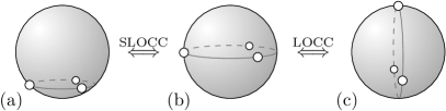
Figure 5.1: The MP distributions of three GHZ-type symmetric states of three qubits are shown. The GHZ-state $\ket{\text{S}_{0}}+\ket{\text{S}_{3}}$ displayed in (b) is LOCC-equivalent to the rotated GHZ-state $\ket{\text{S}_{0}}+\sqrt{3}\ket{\text{S}_{2}}$ shown in (c). The GHZ-type state $\alpha\ket{\text{S}_{0}}+\beta\ket{\text{S}_{3}}$ in (a) is SLOCC-equivalent, but not LOCC-equivalent to the others.

Is it possible to make a similar operational statement with regard to the MP distribution of SLOCC-equivalent symmetric states? From Equation (1.19) and Equation (5.1) it is clear that $\mathcal{B}\in\text{SL}(2,\mathbb{C})$ acts on each MP individually. Therefore, once the action of $\text{SL}(2,\mathbb{C})$ on an individual Bloch vector is understood, one automatically understands how MP distributions transform under the action of symmetric SLOCC operations. Because of $\text{SU}(2)\subset\text{SL}(2,\mathbb{C})$, three of the six d.f. of the special linear group $\text{SL}(2,\mathbb{C})$ can be identified as the usual rotations on the Bloch sphere. From mathematics it is known that the Lie group $\text{SL}(2,\mathbb{C})$ is a double cover of the Möbius group, the automorphism group on the Riemann sphere. Because of this, the transformation of the MPs under a symmetric SLOCC operation is described by a Möbius transformation of complex analysis, with the Majorana sphere in lieu of the Riemann sphere. The Möbius transformations will be covered in detail in Section 5.2, and here we only present the example in Figure 5.1, showing three GHZ-type states that are LOCC or SLOCC-equivalent to each other.

5.1.2 Degeneracy configuration

The Degeneracy Configuration (DC) is an entanglement classification scheme introduced specifically for $n$ qubit symmetric states [82]. Its definition incorporates the Majorana representation by counting the number of identical MPs of a given symmetric state. Each $n$ qubit symmetric state belongs to exactly one DC class $\mathcal{D}_{n_{1},\ldots,n_{d}}$ with $n=n_{1}+\ldots+n_{d}$ ($n_{1}\geq\ldots\geq n_{d}$), and where $n_{1}$ stands for the number of MPs coinciding on one point of the Bloch sphere, $n_{2}$ for those coinciding at a different point, and so on. We call the $n_{i}$ the degeneracy degrees, and the number $d$ the diversity degree. The number of different DC classes into which the Hilbert space of $n$ qubits is partitioned is given by the partition function $p(n)$. The usefulness of the concept of DC classes can be seen from the fact that, due to the non-singular nature of ILOs, the MP degeneracy of a given symmetric state remains invariant under symmetric SLOCC operations: $\ket{\phi_{i}}=\ket{\phi_{j}}\Leftrightarrow\mathcal{B}\ket{\phi_{i}}=\mathcal{B}\ket{\phi_{j}}$ for all $\ket{\phi_{i}},\ket{\phi_{j}}\in\mathbb{C}^{2}$ and all $\mathcal{B}\in\text{SL}(2,\mathbb{C})$. On the other hand, two states that belong to the same DC class do not necessarily belong to the same SLOCC class [82]. Thus we arrive at the following refinement hierarchy:

Theorem 25.

The symmetric subspace of every n qubit Hilbert space has the following refinement hierarchy of entanglement partitions:

$$\text{LOCC}\leq\text{SLOCC}\leq\text{DC}\enspace.$$ (5.3)

An obvious advantage of DC classes over SLOCC classes is that the number of entanglement classes remains finite for arbitrary $n$. This is in stark contrast to the number of SLOCC classes, which becomes infinite for $n\geq 4$ qubits, even when considering only the symmetric subset. Furthermore, operational implications have been found for the concept of DC classes: Each DC class can be unambiguously associated with specific parameter configurations in experiments [82].

5.2 Möbius transformations

As mentioned in the previous section, SLOCC operations between multiqubit symmetric states can be understood by means of the Möbius transformations from complex analysis. This intriguing link was independently discovered and described by me [88] and by Ribeiro and Mosseri [190]. First, the definition of Möbius transformations is recapitulated, and then the transformations are employed to analyse and visualise the freedoms present in symmetric SLOCC operations.

5.2.1 Introduction

The Möbius transformations are defined in complex analysis as the bijective holomorphic functions that project the extended complex plane $\overline{\mathbb{C}}=\mathbb{C}\cup\{\infty\}$ onto itself [111]. These isomorphic functions $f:\overline{\mathbb{C}}\to\overline{\mathbb{C}}$ take the form of rational functions

$$f(z)=\frac{az+b}{cz+d}\enspace,$$ (5.4)

with $a,b,c,d\in\mathbb{C}$, and $ad-bc\neq 0$. The latter condition ensures that $f$ is invertible. In the case $c\neq 0$ the domain of $f$ is $\mathbb{C}\backslash\{-\tfrac{d}{c}\}$ and the codomain is $\mathbb{C}\backslash\{\tfrac{a}{c}\}$, while for $c=0$ both the domain and codomain are $\mathbb{C}$. The extension to a bijective mapping $f:\overline{\mathbb{C}}\to\overline{\mathbb{C}}$ is mediated by $f(-\tfrac{d}{c}):=\infty$, $f(\infty):=\tfrac{a}{c}$ for $c\neq 0$, and $f(\infty):=\infty$ for $c=0$. The coefficients give rise to the matrix representation $\mathcal{B}=\left(\begin{smallmatrix}a&b\\ c&d\end{smallmatrix}\right)$ of the Möbius group, and from Equation (5.4) it is clear that it suffices to consider those $\mathcal{B}$ with determinant one (i.e., $ad-bc=1$). Since $+\mathcal{B}$ and $-\mathcal{B}$ describe the same transformation $f(z)$, the Möbius group is isomorphic to the projective special linear group $\text{PSL}(2,\mathbb{C})=\text{SL}(2,\mathbb{C})/\{\pm\mathbbm{1}\}$.

As outlined in Section 1.3.2, all points of $\overline{\mathbb{C}}$ can be projected onto the Riemann sphere by means of an inverse stereographic projection. With this projection the roots $\{z_{1},\ldots,z_{n}\}$ of the Majorana polynomial (1.25) are projected to the surface of the Majorana sphere, where they become the MPs. The action of a Möbius transformation $f:\overline{\mathbb{C}}\to\overline{\mathbb{C}}$ on the roots $\{z_{1},\ldots,z_{n}\}$ in the extended complex plane then translates on the Majorana sphere to a generalised rotation $\mathcal{B}\in\text{SL}(2,\mathbb{C})$ acting on each MP, which is precisely a symmetric SLOCC operation of the form (5.1). We can therefore view the Möbius transformations (or equivalently symmetric SLOCC operations) either as automorphisms on $\overline{\mathbb{C}}$ or as automorphisms on $\mathcal{S}^{2}$, with the isomorphism between these two manifolds described by the stereographic projection.

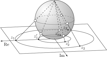
Figure 5.2: A stereographic projection through the north pole of the Majorana sphere mediates between the Majorana roots in the complex plane and the MPs on the surface of the sphere. The SLOCC operation of Figure 5.1 is facilitated by the transformation $f(z)=\tfrac{z}{2}$ which maps the set of roots $\{z_{1},z_{2},z_{3}\}$ onto the set $\{z^{\prime}_{1},z^{\prime}_{2},z^{\prime}_{3}\}$, thus lowering the ring of MPs.

As an example, Figure 5.2 shows the action of the Möbius transformation $f(z)=\tfrac{z}{2}$ which transforms the MPs of the distribution shown in Figure 5.1(b) into that of Figure 5.1(a). It can be seen that circles remain circles under the action of this transformation, both on the sphere and in the complex plane. Intriguingly, this property holds for all Möbius transformations: Both on the Riemann sphere and in the complex plane circles are projected onto circles, where we consider straight lines in the complex plane to be circles too [191]. Furthermore, angles are preserved under Möbius transformations, i.e. two lines or circles that meet at an angle $\alpha$ will still meet at an angle $\alpha$ after the transformation. These properties become more understandable when taking into account that every Möbius transformation (5.4) can be composed from the following elementary operations [111]:

• Rotation & Dilation:  $z\longmapsto az\enspace,$        with $a\in\mathbb{C}\backslash\{0\}$.

  1. Rotation:            $z\longmapsto\text{e}^{\text{i}\varphi}z\enspace,$      with $\varphi\in\mathbb{R}$.

  2. Dilation:             $z\longmapsto rz\enspace,$         with $r>0$.

• Translation:                $z\longmapsto z+b\enspace,$  with $b\in\mathbb{C}$.

• Inversion:                  $z\longmapsto\frac{1}{z}\enspace.$

Möbius transformations can be categorised into different types, depending on the values of the trace and eigenvalues of the transformation matrix $\mathcal{B}$. There exist parabolic, elliptic, hyperbolic and loxodromic Möbius transformations [191], but a unifying feature is that two not necessarily antipodal or distinct points on the Riemann sphere are left invariant. This generalises the $\text{SU}(2)$ rotations, where the two invariant points are the intersections of the rotation axis with the sphere. As an example, the SLOCC operation shown in Figure 5.2 is mediated by a hyperbolic Möbius transformation. These transformations are characterised by the two invariant points (here the north and south pole) acting as attractive and repulsive centres, with the MPs moving away from the repulsive centre towards the attractive one.

A well-known property of Möbius transformations is that for any two ordered sets of three pairwise distinct points $\{v_{1},v_{2},v_{3}\}$ and $\{w_{1},w_{2},w_{3}\}$ there always exists exactly one Möbius transformation that maps one set to the other [191]. This is in general not possible for two sets of four pairwise distinct points, but the cross-ratio preservation of Möbius transformations [191] can be employed to derive a necessary and sufficient condition: An ordered quadruple of distinct complex numbers $\{v_{1},v_{2},v_{3},v_{4}\}$ can be projected onto another quadruple $\{w_{1},w_{2},w_{3},w_{4}\}$ by a Möbius transformation iff

$$\frac{(v_{1}-v_{3})(v_{2}-v_{4})}{(v_{2}-v_{3})(v_{1}-v_{4})}=\frac{(w_{1}-w_{3})(w_{2}-w_{4})}{(w_{2}-w_{3})(w_{1}-w_{4})}\enspace.$$ (5.5)

5.2.2 Relationship to SLOCC operations

From the preceding introduction of the Möbius transformations and Equation (5.1) the following theorem is clear.

Theorem 26.

Two symmetric n qubit states $\ket{\psi^{\text{s}}}$ and $\ket{\phi^{\text{s}}}$ are SLOCC-equivalent iff there exists a Möbius transformation (5.4) between their Majorana roots.

How to determine whether such a Möbius transformation exists? Naturally, $\ket{\psi^{\text{s}}}$ and $\ket{\phi^{\text{s}}}$ must belong to the same DC class, as SLOCC equivalence is a refinement of DC equivalence. One crucial property of Möbius transformations in this regard is that any set of three pairwise distinct points can be projected onto any other. This immediately leads to the following important result, first described in [82].

Corollary 27.

If two symmetric n qubit states $\ket{\psi^{\text{s}}}$ and $\ket{\phi^{\text{s}}}$ belong to the same DC class $\mathcal{D}_{n_{1},\ldots,n_{d}}$ with diversity degree $d\leq 3$, then they are SLOCC-equivalent.

This corollary implies that DC classes with a diversity degree of three or less consist of a single SLOCC class. In particular, this means that for two and three qubit systems the partition into SLOCC classes is the same as the partition into DC classes. The reverse of Corollary 27 clearly does not hold in general, and for states with diversity degree $d=4$ the cross-ratio preservation (5.5) yields the following result:

Corollary 28.

Let $\ket{\psi^{\text{s}}}$ and $\ket{\phi^{\text{s}}}$ be two symmetric n qubit states that belong to the same DC class $\mathcal{D}_{n_{1},\ldots,n_{4}}$ with diversity degree $d=4$. The Majorana roots of $\ket{\psi^{\text{s}}}$ and $\ket{\phi^{\text{s}}}$ corresponding to the degeneracy $n_{i}$ are labelled $v_{i}$ and $w_{i}$, respectively. If the $v_{i}$ and $w_{i}$ fulfil Equation (5.5), then $\ket{\psi^{\text{s}}}$ and $\ket{\phi^{\text{s}}}$ are SLOCC-equivalent.

Note that the ordering of the roots has to be taken into account, because Equation (5.5) does in general not remain true under permutations, and because Majorana roots corresponding to degenerated MPs have to be projected onto Majorana roots with the same degeneracy. In case of a DC class that contains the same degeneracy degree several times, i.e. $n_{i}=n_{j}$ for some $i\neq j$, there is obviously more than one way to designate the indices $n_{i}$ to the roots in decreasing order, and Equation (5.5) needs to hold only for one such ordering to obtain SLOCC-equivalence.

Next we investigate the constituents of SLOCC operations, and identify the freedoms that do not correspond to LOCC operations. The Möbius transformations (5.4) have six real d.f., and are described by $\text{SL}(2,\mathbb{C})$. The polar decomposition of linear algebra states that every invertible complex matrix can be uniquely decomposed into a unitary matrix and a positive-semidefinite Hermitian matrix [193]. We use this result to factorise the d.f. that genuinely belong to SLOCC operations (i.e., which cannot be realized by LOCC operations), and show that this factorisation corresponds to a clear and intuitive visualisation with the Majorana sphere.

Theorem 29.

Every SLOCC operation between two symmetric $n$ qubit states can be factorised into an affine Möbius transformation of the form

$$\widetilde{f}(z)=Az+B\enspace,\quad\text{with}\quad A>0\enspace,\enspace B\in\mathbb{C}\enspace,$$ (5.6)

and an LOCC operation. This decomposition is unique, and the set of transformations (5.6) forms a group that is isomorphic to $\text{SL}(2,\mathbb{C})/\text{SU}(2)$.

Proof.

First, the existence of a factorisation of each SLOCC operation into a transformation $\widetilde{f}$ of the form (5.6) and an LOCC operation is shown. For each $\mathcal{B}=\left(\begin{smallmatrix}a&b\\ c&d\end{smallmatrix}\right)\in\text{SL}(2,\mathbb{C})$ we define $\widetilde{\mathcal{B}}=\lambda\mathcal{B}$ with $\lambda=\sqrt{a{a}^{*}+c{c}^{*}}>0$. Since $\widetilde{\mathcal{B}}$ describes the same SLOCC operation as $\mathcal{B}$, it suffices to show that $\widetilde{\mathcal{B}}$ can be decomposed into an LOCC operation $\mathcal{A}\in\text{SU}(2)$ and a Möbius transformation of the form (5.6):

$$\begin{pmatrix}\lambda a&\lambda b\\ \lambda c&\lambda d\end{pmatrix}=\begin{pmatrix}\alpha&-{\beta}^{*}\\ \beta&{\alpha}^{*}\end{pmatrix}\otimes\begin{pmatrix}A&B\\ 0&1\end{pmatrix}\enspace,$$

with $A>0$ and $\alpha,\beta,B\in\mathbb{C}$, $\alpha{\alpha}^{*}+\beta{\beta}^{*}=1$. For given parameters $a,b,c,d\in\mathbb{C}$ with $ad-bc=1$, this is fulfilled for $\alpha=\frac{a}{\lambda}$, $\beta=\frac{c}{\lambda}$, $A=\lambda^{2}$ and $B=\frac{\lambda^{2}b+{c}^{*}}{a}=\frac{\lambda^{2}d-{a}^{*}}{c}$ (for $a=0$ or $c=0$ only one of the two identities holds). This proves the existence of a factorisation.

To show the uniqueness of factorisations, it is assumed that a given SLOCC operation $\mathcal{B}\in\text{SL}(2,\mathbb{C})$ can be factorised, up to scalar prefactors $\lambda_{1},\lambda_{2}\in\mathbb{C}\backslash\{0\}$, in the above way by two sets of parameters $\{\alpha_{1},\beta_{1},A_{1},B_{1}\}$ and $\{\alpha_{2},\beta_{2},A_{2},B_{2}\}$. Elimination of $\mathcal{B}$ from the resulting matrix equations yields the condition

$$\frac{\lambda_{2}}{\lambda_{1}}\begin{pmatrix}\alpha_{1}&-{\beta}^{*}_{1}\\ \beta_{1}&{\alpha}^{*}_{1}\end{pmatrix}\otimes\begin{pmatrix}A_{1}&B_{1}\\ 0&1\end{pmatrix}=\begin{pmatrix}\alpha_{2}&-{\beta}^{*}_{2}\\ \beta_{2}&{\alpha}^{*}_{2}\end{pmatrix}\otimes\begin{pmatrix}A_{2}&B_{2}\\ 0&1\end{pmatrix}.$$

A straightforward calculation yields $\big{|}\frac{\lambda_{2}}{\lambda_{1}}\big{|}=1$, and from this it readily follows that the two sets of parameters must coincide. This uniqueness implies that the set of transformations $\widetilde{f}$ is isomorphic to $\text{SL}(2,\mathbb{C})/\text{SU}(2)$, and their group properties are easily verified explicitly. ∎

Theorem 29 is closely related to the polar decomposition of matrices, which has also been mentioned in connection with the Bloch sphere in [107]. However, while the matrices describing the affine transformations $\widetilde{f}$ are positive, they are in general not Hermitian (unlike in the polar decomposition), and the introduction of the prefactor $\lambda$ in the proof is necessary because $\mathcal{A}$ and $\mathcal{B}$ are defined to have unit determinants.

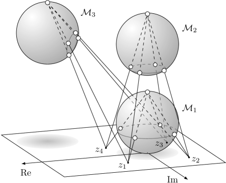
Figure 5.3: Alternative visualisation of Möbius transformations where a fixed set of complex points is projected onto the surface of a moving sphere. The three innate freedoms of SLOCC operations not present in LOCC operations are then described by the translations of the Majorana sphere in $\mathbb{R}^{3}$. The north pole of sphere $\mathcal{M}_{1}$ (with the MP distribution of the five qubit “square pyramid state”) lies 2 units above the origin of the complex plane, while the one of $\mathcal{M}_{2}$ lies 5 units above, and $\mathcal{M}_{3}$ is additionally displaced horizontally by a vector $5-5\text{i}$. The parameters $(A,B)$ of Equation (5.6) for the transformation of $\mathcal{M}_{1}$ to $\mathcal{M}_{2}$ and $\mathcal{M}_{3}$ are $(\tfrac{5}{2},0)$ and $(\tfrac{5}{2},5-5\text{i})$, respectively.

The orthodox way to visualise Möbius transformations is to fix the Riemann sphere in $\mathbb{R}^{3}$, and points $\{z_{1},\ldots,z_{n}\}$ on the complex plane are transformed to different points $\{z^{\prime}_{1},\ldots,z^{\prime}_{n}\}$ under the action of (5.4). Alternatively, the points in the plane can be considered fixed, and instead the Riemann sphere moves in $\mathbb{R}^{3}$, as shown in Figure 5.3. The six d.f. of the Möbius transformations are then split into three translational freedoms (movement of sphere in $\mathbb{R}^{3}$) and three rotational freedoms ($\text{SU}(2)$-rotations of sphere). By considering these elementary operations it can be verified by calculation that this is an equivalent way of viewing the change of MPs on the sphere under the action of Möbius transformations. A general SLOCC operation between two symmetric states is then described by a translation of the Majorana sphere in $\mathbb{R}^{3}$, followed by a rotation. In this approach the affine transformations (5.6) exactly describe the set of translations in $\mathbb{R}^{3}$ that leave the sphere’s north pole above the complex plane. The parameters of the affine function $\widetilde{f}(z)=Az+B$ correspond to the translation as follows: The parameter $A=\tfrac{h_{2}}{h_{1}}$ is the ratio of the heights of the north pole before ($h_{1}$) and after ($h_{2}$) the transformation, and $B$ is the horizontal displacement vector (cf. Figure 5.3). Regarding the subsequent rotation of the Majorana sphere, it is clear that it leaves the relative MP distribution invariant and can be described by an LOCC operation.

5.3 Representative states for SLOCC classes

In the following the SLOCC and DC classes of symmetric states of up to $5$ qubits are characterised, and representative states are given for each equivalence class. The aim is to provide representations that are not only unique (i.e. the representative states are all inequivalent to each other), but that also allow for a simple analytical form as well as simple MP distributions. Before tackling this problem, we briefly investigate the relationship between general and symmetric states under SLOCC operations. For example, if it were possible to transform every nonsymmetric state into a symmetric state by SLOCC, then the restriction to symmetric states would be merely an artificial one, because all states in $\mathcal{H}$ could be represented by symmetric states.

5.3.1 Relationship between symmetric and nonsymmetric states

From a comparison of parameters it can be easily seen that the aforementioned symmetrisation of generic states by SLOCC operations is a rare exception: Unnormalised pure states of $n$ qubits are described by $2^{n}$ complex coefficients, and taking the global phase into account, this leads to $2^{n+1}-1$ independent real degrees of freedom (d.f.). General SLOCC operations (which include LU operations that can be associated with basis transformations and standard forms) are described by $\text{SL}(2,\mathbb{C})^{n}$ and have $6n$ real d.f., so the number of remaining independent d.f. is $2^{n+1}-6n-1$. On the other hand, unnormalised symmetric $n$ qubit states are described by $n+1$ Dicke states, yielding $2(n+1)-1$ independent real freedoms. Since $2^{n+1}-6n-1\leq 2(n+1)-1$ holds only for $n\leq 4$ qubits, it is clear that generic states of five and more qubits cannot be symmetrised by SLOCC. In Section 1.2.3 the SLOCC equivalence classes of systems with up to four qubits were already reviewed, and we will now follow up on this by investigating whether these equivalence classes contain symmetric states.

First, we note that the symmetrisation of the SLOCC class of $n$ qubit product states is trivial, because every product state can be turned into a symmetric state (e.g. $\ket{0}^{\otimes n}$) by an LU operation. This SLOCC class coincides with the DC class $\mathcal{D}_{n}$.

The other extreme with regard to symmetrisation are the SLOCC classes with states that are neither product states nor entangled over all parties. As an example, the three qubit state $\ket{\psi}_{\text{A-BC}}=\ket{000}+\ket{011}=\ket{0}\otimes(\ket{00}+\ket{11})$ is biseparable, because the first qubit is not entangled with the rest. This inherently asymmetric property cannot be lifted by SLOCC operations, since local operations cannot create entanglement over disentangled parts. Thus the SLOCC class to which $\ket{\psi}_{\text{A-BC}}$ belongs does not contain a single symmetric state. As symmetric states are either fully separable or entangled over all parties [194], this implies that for three and more qubits there always exist fundamentally nonsymmetric SLOCC classes.

Every pure bipartite state (which includes the 2 qubit case) can be cast as a symmetric state by means of the Schmidt decomposition (1.6), which means that every state is LU-equivalent to a symmetric state. For 2 qubits there are two SLOCC equivalence classes, containing the separable and entangled states, respectively. Choosing the states $\ket{\text{S}_{0}}$ and $\ket{\text{S}_{1}}$ as representatives of these SLOCC classes, we display their Majorana representations in Figure 5.4.

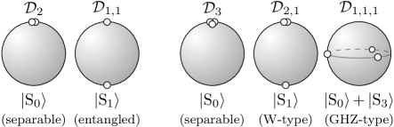
Figure 5.4: The SLOCC and DC classes of 2 and 3 qubit symmetric states are represented by the MP distributions of characteristic states. Because of Corollary 27 each DC class consists of a single SLOCC class. Excluding the biseparable 3 qubit states, every 2 or 3 qubit state can be transformed into one of the symmetric states shown here by a (generally nonsymmetric) SLOCC operation.

For 3 qubits there exist six different SLOCC classes, the separable class, the three biseparable classes, and the two inequivalent classes with GHZ-type and W-type entanglement [18, 195]. All states of the latter two classes are SLOCC-equivalent to the $\ket{\text{GHZ}}$ and $\ket{\text{W}}$ state, respectively [18]. Therefore, with the exception of the biseparable states, every three qubit state can be turned into a symmetric state by SLOCC. In Figure 5.4 the three symmetric SLOCC classes are represented by the states $\ket{\text{S}_{0}}$, $\ket{\text{S}_{1}}$ and $\ket{\text{S}_{0}}+\ket{\text{S}_{3}}$. From Corollary 27 it is clear that the DC classes coincide with the SLOCC classes, with $\mathcal{D}_{3}$ containing the separable states, $\mathcal{D}_{2,1}$ the W-type entangled states and $\mathcal{D}_{1,1,1}$ the GHZ-type entangled states.

For 4 qubits the number of SLOCC classes becomes infinite [18], even when considering only the subset of symmetric states. The symmetric entanglement classes of 4 qubits will be investigated in detail in the next section, and in Section 5.4 these classes will be linked to the Entanglement Families (EF) of Verstraete et al. [51].

5.3.2 Four qubit symmetric classes

For symmetric states of 4 qubits there exist five DC classes and a continuum of SLOCC classes [82]. As shown in Figure 5.5, four of the DC classes coincide with SLOCC classes (which is clear from Corollary 27), while the generic class $\mathcal{D}_{1,1,1,1}$ with no MP degeneracy is comprised of a continuum of SLOCC classes (cf. Figure 2 in [85]). We will now parameterise this continuum in a way that exactly one state, acting as the representative state, is chosen from every SLOCC class. The high symmetry present in an equidistant distribution of three MPs along the equator facilitates the restriction of the remaining MP to a well-defined, connected area on the sphere’s surface:

Theorem 30.

Every pure symmetric state of 4 qubits is SLOCC-equivalent to exactly one state of the set

$$\{\ket{\text{S}_{0}},\,\ket{\text{S}_{1}},\,\ket{\text{S}_{2}},\,2\ket{\text{S}_{0}}+t\ket{\text{S}_{1}}+\ket{\text{S}_{3}}+2t\ket{\text{S}_{4}}\}\enspace,$$

$$\text{with}\quad t=\text{e}^{\text{i}\varphi}\tan\tfrac{\theta}{2}\enspace,\quad\text{and}\quad(\theta,\varphi)\in\bm{\{}[0,\tfrac{\pi}{2})\times[0,\tfrac{2\pi}{3})\bm{\}}\cup\bm{\{}\{\tfrac{\pi}{2}\}\times[0,\tfrac{\pi}{3}]\bm{\}}\enspace.$$

Proof.

First it will be shown that every symmetric 4 qubit state $\ket{\psi^{\text{s}}}$ can be transformed by SLOCC into one of the above states. From the previous discussion and Figure 5.5, this is clear for all DC classes except $\mathcal{D}_{1,1,1,1}$. Given an arbitrary state $\ket{\psi^{\text{s}}}\in\mathcal{D}_{1,1,1,1}$, there always exists a Möbius transformation $f:\ket{\psi^{\text{s}}}\mapsto\ket{\psi^{\prime\text{s}}}$ s.t. three MPs are projected onto the three corners of an equilateral triangle in the equatorial plane. If the fourth MP $\ket{\phi_{4}}$ is not projected into the area parameterised by $(\theta,\varphi)\in\bm{\{}[0,\tfrac{\pi}{2})\times[0,\tfrac{2\pi}{3})\bm{\}}\cup\bm{\{}\{\tfrac{\pi}{2}\}\times(0,\tfrac{\pi}{3}]\bm{\}}$ (cf. Figure 5.5), then it can be projected into that area by a combination of $\{\operatorname{R_{x}^{s}}(\pi),\operatorname{R_{z}^{s}}(\tfrac{2\pi}{3})\}$-rotations which preserve the equatorial MP distribution.

It remains to show that this set of states is unique, i.e., two different MPs $\ket{\phi_{4}}$ and $\ket{\phi_{4}^{\prime}}$ within the aforementioned parameter range give rise to two different states $\ket{\psi^{\text{s}}}\neq\ket{\psi^{\prime\text{s}}}$ which are SLOCC-inequivalent. By considering all 4! possible projections between the MPs of $\ket{\psi^{\text{s}}}$ and $\ket{\psi^{\prime\text{s}}}$ it can be easily verified explicitly with the cross-ratio preservation (5.5) that a transformation is possible only if $\ket{\phi_{4}}=\ket{\phi_{4}^{\prime}}$. ∎

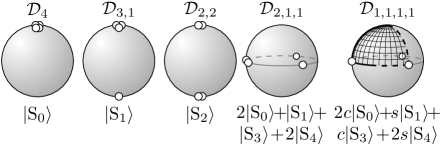
Figure 5.5: Only four of the five DC classes of 4 qubit symmetric states coincide with a single SLOCC class. Due to the continuum of SLOCC classes present in $\mathcal{D}_{1,1,1,1}$, only three MPs can be fixed in its representative state, with the unique locations for the fourth MP $c\ket{0}+s\ket{1}$ parameterising the set of representative states. Here $c=\cos\tfrac{\theta}{2}$ and $s=\text{e}^{\text{i}\varphi}\sin\tfrac{\theta}{2}$, and the range of parameters is $(\theta,\varphi)\in\bm{\{}[0,\tfrac{\pi}{2})\times[0,\tfrac{2\pi}{3})\bm{\}}\cup\bm{\{}\{\tfrac{\pi}{2}\}\times(0,\tfrac{\pi}{3}]\bm{\}}$, shown as a black grid. The fixed equatorial MPs of the representative states are equidistantly spaced.

5.3.3 Five qubit symmetric classes

The DC classes of 5 qubits and representative states for the SLOCC classes can be seen in Figure 5.6. The SLOCC classes of the generic class $\mathcal{D}_{1,1,1,1,1}$ can be parameterised by two complex variables, corresponding to two MPs in the black and white area, respectively. Unlike the 4 qubit case, however, this parameterisation is neither unique, nor confined to the generic DC class. Different sets of parameters $(\theta_{1},\varphi_{1},\theta_{2},\varphi_{2})\neq(\theta^{\prime}_{1},\varphi^{\prime}_{1},\theta^{\prime}_{2},\varphi^{\prime}_{2})$ can give rise to SLOCC-equivalent states, and for $(\theta_{1},\varphi_{1})=(\theta_{2},\varphi_{2})$ the corresponding state does not even belong to $\mathcal{D}_{1,1,1,1,1}$ because of an MPs degeneracy. A unique set of representative states can therefore be provided only for the subset of symmetric states with at least one MP degeneracy:

Theorem 31.

Every pure symmetric state of 5 qubits with an MP degeneracy (i.e., diversity degree $d<5$) is SLOCC-equivalent to exactly one state of the set

$$\{\ket{\text{S}_{0}},\,\ket{\text{S}_{1}},\,\ket{\text{S}_{2}},\,\sqrt{10}\left(\ket{\text{S}_{0}}+t\ket{\text{S}_{5}}\right)+t\ket{\text{S}_{2}}+\ket{\text{S}_{3}}+\sqrt{2}\left(1+t\right)\left(\ket{\text{S}_{1}}+\ket{\text{S}_{4}}\right)\}\enspace,$$

$$\text{with}\quad t=\text{e}^{\text{i}\varphi}\tan\tfrac{\theta}{2}\enspace,\quad\text{and}\quad(\theta,\varphi)\in\bm{\{}[0,\tfrac{\pi}{2})\times[0,2\pi)\bm{\}}\cup\bm{\{}\{\tfrac{\pi}{2}\}\times[0,\pi]\bm{\}}\enspace.$$

Proof.

The proof runs analogous to the one of Theorem 30, with the observation that the representative states of the $\mathcal{D}_{3,1,1}$ and $\mathcal{D}_{2,2,1}$ class are readily subsumed in the parameter range of $\mathcal{D}_{2,1,1,1}$. The fixed MPs of $\mathcal{D}_{2,1,1,1}$ are left invariant under a $\operatorname{R_{x}^{s}}(\pi)$-rotation, thus ensuring that the remaining MP can be projected into the desired parameter range. The uniqueness is again verified by considering all possible cross-ratios. ∎

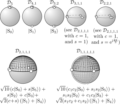
Figure 5.6: The first five of the seven DC classes of 5 qubit symmetric states coincide with SLOCC classes, while the representative states of $\mathcal{D}_{2,1,1,1}$ are parameterised by one MP $c\ket{0}+s\ket{1}$ (black grid), and those of $\mathcal{D}_{1,1,1,1,1}$ by two MPs (black and white grid). The parameter range for $\mathcal{D}_{2,1,1,1}$ is $(\theta,\varphi)\in\bm{\{}[0,\tfrac{\pi}{2})\times[0,2\pi)\bm{\}}\cup\bm{\{}\{\tfrac{\pi}{2}\}\times(0,\pi]\bm{\}}\backslash\bm{\{}\{\tfrac{\pi}{2}\}\times\{\tfrac{2\pi}{3}\}\bm{\}}$. For $\mathcal{D}_{1,1,1,1,1}$ the range of $(\theta_{1},\varphi_{1})$ is the same as $(\theta,\varphi)$, and $(\theta_{2},\varphi_{2})\in\bm{\{}[0,\pi]\times[0,\tfrac{2\pi}{3})\bm{\}}\backslash\bm{\{}\{\tfrac{\pi}{2}\}\times\{0\}\bm{\}}$. The fixed equatorial MPs of the representative states are all equidistantly spaced.

An over-complete set of representative states for the general case can be given as follows:

Corollary 32.

Every pure symmetric state of 5 qubits is SLOCC-equivalent to one or more state of the set

$$\{\ket{\text{S}_{0}},\,\ket{\text{S}_{1}},\,\ket{\text{S}_{2}},\,\sqrt{10}\left(\ket{\text{S}_{0}}+t_{1}t_{2}\ket{\text{S}_{5}}\right)+t_{1}t_{2}\ket{\text{S}_{2}}+\ket{\text{S}_{3}}+\sqrt{2}\left(t_{1}+t_{2}\right)\left(\ket{\text{S}_{1}}+\ket{\text{S}_{4}}\right)\}\enspace,$$

$$\text{with}\quad t_{i}=\text{e}^{\text{i}\varphi_{i}}\tan\tfrac{\theta_{i}}{2}\enspace,\quad\text{and}\quad(\theta_{1},\varphi_{1}) \in\bm{\{}[0,\tfrac{\pi}{2}]\times[0,2\pi)\bm{\}}\cup\bm{\{}\{\tfrac{\pi}{2}\}\times(0,\pi]\bm{\}}\enspace,$$

$$(\theta_{2},\varphi_{2}) \in\bm{\{}[0,\pi]\times[0,\tfrac{2\pi}{3})\bm{\}}\enspace.$$

Proof.

Only the generic class $\mathcal{D}_{1,1,1,1,1}$ needs to be considered. Given an arbitrary state of this class, three of its MPs can be projected onto the vertices of an equilateral triangle by means of a Möbius transformation. These MPs are left invariant under $\{\operatorname{R_{x}^{s}}(\pi),\operatorname{R_{z}^{s}}(\tfrac{2\pi}{3})\}$-rotations. If the fourth MP does not lie in the $(\theta_{1},\varphi_{1})$-area, it can be projected there by a $\operatorname{R_{x}^{s}}(\pi)$-rotation. Subsequent $\operatorname{R_{z}^{s}}(\tfrac{2\pi}{3})$-rotations can project the fifth MP into the $(\theta_{2},\varphi_{2})$-area, while leaving the fourth MP in the $(\theta_{1},\varphi_{1})$-area. ∎

As the number of qubits increases, the picture gradually becomes more complicated, because DC classes with diversity degree $n$ contain a continuous range of SLOCC classes that is parameterised by $n-3$ variables [82].

5.4 Entanglement families of four qubits

The concept of Entanglement Families (EF) was already briefly touched upon in Section 1.2.3. Derived by Verstraete et al. [51] with some advanced methods of linear algebra, this classification scheme reduces the complexity of the four qubit case by replacing the infinite amount of SLOCC classes with nine different EF. The EF a state belongs to does not change under SLOCC operations, thus making the partition into SLOCC classes a refinement of the partition into EF classes (SLOCC $\leq$ EF). The nine EF are represented by the following ranges of states, with $a,b,c,d\in\mathbb{C}$ being arbitrary complex parameters.

• $G_{abcd}=\frac{a+d}{2}\big{(}\ket{0000}+\ket{1111}\big{)}+\frac{a-d}{2}\big{(}\ket{0011}+\ket{1100}\big{)}+\frac{b+c}{2}\big{(}\ket{0101}+\ket{1010}\big{)}\\ \hskip 48.36958pt+\frac{b-c}{2}\big{(}\ket{0110}+\ket{1001}\big{)}$

• $L_{abc_{2}}=\frac{a+b}{2}\big{(}\ket{0000}+\ket{1111}\big{)}+\frac{a-b}{2}\big{(}\ket{0011}+\ket{1100}\big{)}+c\big{(}\ket{0101}+\ket{1010}\big{)}+\ket{0110}$

• $L_{a_{2}b_{2}}=a\big{(}\ket{0000}+\ket{1111}\big{)}+b\big{(}\ket{0101}+\ket{1010}\big{)}+\ket{0110}+\ket{0011}$

• $L_{ab_{3}}=a\big{(}\ket{0000}+\ket{1111}\big{)}+\frac{a+b}{2}\big{(}\ket{0101}+\ket{1010}\big{)}+\frac{a-b}{2}\big{(}\ket{0110}+\ket{1001}\big{)}\\ \hskip 48.36958pt+\frac{\text{i}}{\sqrt{2}}\big{(}\ket{0001}+\ket{0010}+\ket{0111}+\ket{1011}\big{)}$

• $L_{a_{4}}=a\big{(}\ket{0000}+\ket{0101}+\ket{1010}+\ket{1111}\big{)}+\big{(}\text{i}\ket{0001}+\ket{0110}-\text{i}\ket{1011}\big{)}$

• $L_{a_{2}0_{3\oplus\bar{1}}}=a\big{(}\ket{0000}+\ket{1111}\big{)}+\big{(}\ket{0011}+\ket{0101}+\ket{0110}\big{)}$

• $L_{0_{5\oplus\bar{3}}}=\ket{0000}+\ket{0101}+\ket{1000}+\ket{1110}$

• $L_{0_{7\oplus\bar{1}}}=\ket{0000}+\ket{1011}+\ket{1101}+\ket{1110}$

• $L_{0_{3\oplus\bar{1}}0_{3\oplus\bar{1}}}=\ket{0000}+\ket{0111}$

Up to permutations, every pure 4 qubit state is SLOCC-equivalent to a state from exactly one of these families. Unlike in our Theorem 30, however, the parameterisation of the EF is not unique, i.e. two different sets of parameters $(a,b,c,d)\neq(a^{\prime},b^{\prime},c^{\prime},d^{\prime})$ can give rise to two SLOCC-equivalent states. This non-uniqueness can be already seen from the non-normalised nature of the generic family $G_{abcd}$ which is due to the choice of the parameters $a,b,c,d$ as the eigenvalues of a matrix employed for the proof in [51]. A less trivial example are the two symmetric states $\ket{\psi^{a}}=\ket{\text{S}_{2}}$ and $\ket{\psi^{b}}=(\ket{\text{S}_{0}}+\ket{\text{S}_{4}})+\sqrt{\tfrac{2}{3}}\ket{\text{S}_{2}}$ which are both present in the family $G_{abcd}$. Their LU equivalence $\ket{\psi^{a}}\stackrel{{\scriptstyle\text{LU}}}{{\longleftrightarrow}}\ket{\psi^{b}}$ can be immediately seen from their MP distributions $\ket{\phi^{a}_{1,2}}=\ket{0}$, $\ket{\phi^{a}_{3,4}}=\ket{1}$, and $\ket{\phi^{b}_{1,2}}=\tfrac{1}{\sqrt{2}}(\ket{0}+\text{i}\ket{1})$, $\ket{\phi^{b}_{3,4}}=\tfrac{1}{\sqrt{2}}(\ket{0}-\text{i}\ket{1})$.

Here we are interested in the subset of symmetric 4 qubit states. In the following we will determine in which EF the symmetric SLOCC classes are located, and we will elucidate the relationship between the DC and EF classes, both of which are coarser partitions than the SLOCC classes.

First, we identify the EF of the SLOCC and DC classes shown in Figure 5.5. The separable state $\ket{\text{S}_{0}}$, and therefore the entire $\mathcal{D}_{4}$ class, is LU-equivalent to the state $\ket{0110}$ embedded in the family $L_{{abc}_{2}}$ for parameters $a=b=c=0$. The W state $\ket{\text{S}_{1}}$ representing $\mathcal{D}_{3,1}$ is recovered from the family $L_{{ab}_{3}}$ by setting $a=b=0$ and spin-flipping the last two qubits. The state $\ket{\text{S}_{2}}$ representing $\mathcal{D}_{2,2}$ can be found in the general family $G_{abcd}$ by setting $a=1,b=2,c=0,d=-1$. A state of the degeneracy class $\mathcal{D}_{2,1,1}$ is found in $L_{{abc}_{2}}$ by setting $a=1,b=0,c=\tfrac{1}{2}$ and spin-flipping the second and third qubit, yielding the state $\ket{\psi}=\sqrt{\tfrac{2}{5}}\ket{\text{S}_{0}}+\sqrt{\tfrac{3}{5}}\ket{\text{S}_{2}}$ which is made up of the MPs $\ket{\phi_{1,2}}=\ket{0}$ and $\ket{\phi_{3,4}}=\tfrac{1}{2}\ket{0}\pm\text{i}\tfrac{\sqrt{3}}{2}\ket{1}$. The continuum of SLOCC classes present in the generic class $\mathcal{D}_{1,1,1,1}$ has previously been parameterised in [82] as $\left(\ket{\text{S}_{0}}+\ket{\text{S}_{4}}\right)+\mu\ket{\text{S}_{2}}$, with $\mu\in\mathbb{C}\backslash\{\pm\sqrt{\tfrac{2}{3}}\}$. These states are recovered from the general family $G_{abcd}$ for $a=1+\tfrac{\mu}{\sqrt{6}},b=\sqrt{\tfrac{2}{3}}\mu,c=0,d=1-\tfrac{\mu}{\sqrt{6}}$. The reason for the exclusion of $\mu=\pm\sqrt{\tfrac{2}{3}}$ is that the MP distribution then becomes degenerate, and it was already seen above that $\ket{\psi^{b}}=\left(\ket{\text{S}_{0}}+\ket{\text{S}_{4}}\right)+\sqrt{\tfrac{2}{3}}\ket{\text{S}_{2}}$ is LU-equivalent to $\ket{\text{S}_{2}}\in\mathcal{D}_{2,2}$. Summing up, we found

• $\mathcal{D}_{1,1,1,1}$, $\mathcal{D}_{2,2}\subset G_{abcd}$

• $\mathcal{D}_{2,1,1}$, $\mathcal{D}_{4}\subset L_{{abc}_{2}}$

• $\mathcal{D}_{3,1}\subset L_{{ab}_{3}}$

In particular, only three of the nine EF contain all the states of the symmetric subspace of the 4 qubit Hilbert space, including those non-symmetric states that are SLOCC-equivalent to symmetric states. The other six EF only contain genuinely non-symmetric states that cannot be symmetrised by SLOCC operations. Furthermore, it is noteworthy that the families $G_{abcd}$ and $L_{{abc}_{2}}$ each contain two different DC classes. This is somewhat unexpected, because there exist nine different EF, but only five different DC classes. We can therefore conclude that the EF are not a particularly useful classification scheme for symmetric states, due to their coarseness. Since all states of a given DC class are contained in only one EF, Theorem 25 can be specified for the 4 qubit case:

Theorem 33.

The symmetric subspace of the 4 qubit Hilbert space has the following refinement hierarchy of entanglement partitions:

$$\text{LOCC}<\text{SLOCC}<\text{DC}<EF\enspace.$$ (5.7)

5.5 Determining SLOCC inequivalence from the
MP distribution

The known properties of Möbius transformations can be employed to immediately determine whether two symmetric $n$ qubit states with the same degeneracy of their MPs could be SLOCC-equivalent. As outlined in Section 5.2.1, circles on the surface of the Majorana sphere are always projected onto circles, and the angles at which two circles meet are preserved. These properties can be exploited by identifying and comparing circles with MPs on them.

As an example, Figure 5.7 shows the MP distributions of some states investigated in Chapter 4. The two 5 qubit states $\ket{\psi_{5}}$ and $\ket{\Psi_{5}}$ are not SLOCC-equivalent, because $\ket{\Psi_{5}}$ exhibits a ring with four MPs, whereas no ring with four MPs can be found for $\ket{\psi_{5}}$. Similarly, it can be shown that most of the states investigated in Chapter 4 are SLOCC-inequivalent to each other. For 12 qubits it is not immediately clear that the positive solution $\ket{\psi_{12}}$ and the icosahedron state $\ket{\Psi_{12}}$, shown in Figure 5.7, are SLOCC-inequivalent, since both states have several rings with four or five MPs each. In the icosahedron state $\ket{\Psi_{12}}$ it is possible to identify 20 circles, each through three adjacent MPs (the corners of all faces of the icosahedron), so that the interior of each circle is free of MPs. This property must be preserved under Möbius transformations, but for $\ket{\psi_{12}}$ it is not possible to find such twenty distinct circles that are all free of MPs in their interior.

\begin{overpic}[scale={1.3}]{figure5_7} \put(-1.0,0.0){(a)} \put(24.0,0.0){(b)} \put(53.0,0.0){(c)} \put(77.0,0.0){(d)} \end{overpic}

Figure 5.7: The MP distributions of four highly or maximally entangled symmetric states introduced in Chapter 4 are shown. The 5 qubit “trigonal bipyramid state” $\ket{\psi_{5}}$ is SLOCC-inequivalent to the “square pyramid state” $\ket{\Psi_{5}}$. Likewise, the 12 qubit icosahedron state $\ket{\Psi_{12}}$ cannot be reached from $\ket{\psi_{12}}$ by SLOCC operations.

Markham [85] determined the SLOCC-inequivalence of the four qubit GHZ state $\ket{\text{GHZ}_{4}}$ and tetrahedron state $\ket{\text{T}}$ analytically from the values of their Schmidt rank and geometric entanglement. Interestingly, with the geometrically motivated approach employed here there is no need for such calculations: The MPs of $\ket{\text{GHZ}_{4}}$ all lie on the single ring, but those of $\ket{\text{T}}$ don’t.

The SLOCC-inequivalence of all totally invariant states of up to 7 qubits was determined in [85] by considering the MP degeneracies as well as the Schmidt rank, and a conjecture was made that all totally invariant symmetric states are SLOCC-inequivalent to each other. Using the preservation of circles and angles under Möbius transformations, it is expected that this conjecture becomes much easier to verify.

The existence of $n$ qubit states that are not LOCC or SLOCC-equivalent to their complex conjugates has been affirmed [39, 43], and the operational consequences of this for distinguishing such states have been discussed [43, 196]. Taking the complex conjugation into account, the number of parameters to describe pure three qubit states up to LU were reduced from six to five [196]. In the case of symmetric states we immediately see that complex conjugation corresponds to a reflection of the MPs along the $X$-$Z$-plane. We can therefore explain the LOCC-inequivalence of complex conjugate symmetric states with the geometric concept of chirality, or handedness: Although having the same distances and angles (and therefore the same geometric entanglement), the mirror image of an arbitrary MP distribution is in general not LU-equivalent to the original. This idea can be easily extended to SLOCC-equivalence, with the result that general symmetric states are not even SLOCC-equivalent to their complex conjugate.

5.6 Symmetric SLOCC invariants on the Majorana sphere

We are already familiar with the property of Möbius transformations to preserve circles and angles, as well as the cross-ratios (5.5) of ordered quadruples of points. These quantities can therefore be considered to be symmetric SLOCC invariants.

A detailed study of symmetric LU and SLOCC invariants with the Majorana representation was recently undertaken by Ribeiro and Mosseri [190]. With regard to symmetric LU operations (which are equivalent to LOCC operations between symmetric states, cf. Equation (5.2)), they found that the well-known six LU invariants for 3 qubits [197, 50] can be expressed in terms of the $3!$ angles between pairs of MPs. With regard to symmetric SLOCC operations, the cross-ratios were identified as a natural basis for invariants. Given a cross-ratio,

$$\lambda:=\frac{(v_{1}-v_{3})(v_{2}-v_{4})}{(v_{2}-v_{3})(v_{1}-v_{4})}\in\overline{\mathbb{C}}\enspace,$$ (5.8)

the $24$ different possible ways to permute the entries $\{v_{1},v_{2},v_{3},v_{4}\}$ generally leads to six different values $\{\lambda_{i}\}$ for the cross ratio: $\{\lambda,\tfrac{1}{\lambda},1-\lambda,\tfrac{1}{1-\lambda},\tfrac{\lambda}{\lambda-1},\tfrac{\lambda-1}{\lambda}\}$ [190]. These different values partition the complex plane into six distinct regions, as seen in Figure 5.8(b).

\begin{overpic}[scale={1.3}]{figure5_8_a} \put(-12.0,0.0){(a)} \put(31.0,155.0){$\mathcal{D}_{1,1,1,1}$} \put(15.0,127.0){$2c\ket{\text{S}_{0}}+s\ket{\text{S}_{1}}+$} \put(18.0,107.0){$c\ket{\text{S}_{3}}+2s\ket{\text{S}_{4}}$} \end{overpic}\begin{overpic}[scale={0.9}]{figure5_8_b} \put(0.0,0.0){(b)} \end{overpic}

\begin{overpic}[scale={1.02}]{figure5_8_c} \put(2.0,3.0){(c)} \end{overpic}

Figure 5.8: An alternative parameterisation of the generic 4 qubit DC class $\mathcal{D}_{1,1,1,1}$ is shown in (a), with the parameterisation of the fourth MP $c\ket{0}+s\ket{1}$ being $(\theta,\varphi)\in\bm{\{}[0,\pi)\times[0,\tfrac{\pi}{3})\bm{\}}$. The six different areas $\{\lambda_{i}\}$ in the complex plane that correspond to permutations of the entries in Equation (5.8) are shown in (b). The plane is cut by the line $\operatorname{Re}(z)=\tfrac{1}{2}$, as well as two unit circles with centres $z=0$ and $z=1$. Aligning the poles of the sphere (a) with the points $z=\frac{1}{2}+\text{i}$ and $z=\frac{1}{2}-\text{i}$ in (b) yields the arrangement (c), which can be understood as a stereographic projection of the parameter range $(\theta,\varphi)$ onto one of the six areas $\{\lambda_{i}\}$.

Here we point out a relationship of this partition to the generic SLOCC equivalence classes of 4 qubits, namely the degeneracy class $\mathcal{D}_{1,1,1,1}$ studied in Section 5.3.2. The parameter range chosen for the unique representative states of $\mathcal{D}_{1,1,1,1}$ in Figure 5.5 is not the only possibly choice, and an equivalent parameterisation with a high degree of symmetry is shown in Figure 5.8(a). There the fourth MP $\ket{\phi_{4}}=c\ket{0}+s\ket{1}$ has the parameterisation $(\theta,\varphi)\in\bm{\{}[0,\pi)\times[0,\tfrac{\pi}{3})\bm{\}}$. As shown in Figure 5.8, this parameter range can be projected onto one of the six areas $\{\lambda_{i}\}$ in the complex plane by means of a stereographic projection. This is by no means a coincidence, but rather a consequence of SLOCC invariants: Every value within the parameter range of $(\theta,\varphi)$ corresponds to a unique state that is SLOCC-inequivalent to any other value within that range. Likewise, two 4 qubit symmetric states with no MP degeneracies are SLOCC-inequivalent iff the cross-ratios (5.8) of their Majorana roots are different for all possible permutations, which implies that the values of their cross-ratios need to be considered only for one of the six areas $\{\lambda_{i}\}$.

5.7 Global entanglement measures

Polynomial SLOCC invariants that provide information about the type of entanglement present in a system were already mentioned at the end of Section 1.2.3. Here we review two well-known approaches in light of our results about symmetric states.

5.7.1 Maximal $n$-tangles

Osterloh and Siewert [58, 59] constructed entanglement monotones from antilinear operators that are invariant under SLOCC operations, and that can be understood as generalisations of the concurrence (2-tangle) [56] and the 3-tangle [50]. This allows for the construction of a “global entanglement measure” with the aim to detect only genuine $n$ qubit entanglement in the sense that it is blind for $k$-partite entanglement with $k<n$. More formally, an $n$ qubit state $\ket{\Psi_{n}}$ is a “maximal $n$-tangle” if the following two conditions hold [58, 59, 198]:

1. All reduced density matrices of $\ket{\Psi_{n}}$ with rank $\leq 2$ are maximally mixed.

2. All $k$-site reduced density matrices of $\ket{\Psi_{n}}$ have zero $k$-tangle ($1<k<n$).

This definition of maximal entanglement is very similar to those proposed in [184, 41]. The first condition implies that a maximal amount of information is gained when reading out a qubit, something that is closely related to the stochastic states of [41]. The second condition excludes hybrids of various types of entanglement, thus following the concept of monogamy [50], i.e. that the total entanglement is a resource distributed among different types of entanglement. Occasionally, a third condition is imposed, namely that the maximally $n$-tangled states have a phase-independent canonical form, i.e. that the first two properties shall be unaffected by relative phases in the coefficients [59]. This implies that maximally $n$-tangled states can always be written with positive coefficients, which is quite interesting for us because of our focus on positive states. On the other hand, this is a first indication that “global entanglement measures” are qualitatively different from e.g. the geometric measure, because the latter is not expected to be maximised for positive states in general. Another interesting property of global entanglement measures is that they are closely related to the concept of symmetry, in the sense that permutational invariance was identified as a characteristic property of such measures [50].

The $n$ qubit GHZ state is a maximally $n$-tangled state for all $n$, and in the case of 3 qubits it is the only such state. Therefore the SLOCC class of 3 qubit states with genuine tripartite entanglement is represented by the GHZ state.

Another maximally $n$-tangled state for every $n\geq 3$ is the following state,

$$\ket{X_{n}}=\sqrt{n}\ket{\text{S}_{1}}+\sqrt{n-2}\ket{\text{S}_{n}}\enspace,$$ (5.9)

coined the X-state [198]. Note that in the 3 qubit case the state $\ket{X_{3}}$ is LU-equivalent to $\ket{\text{GHZ}_{3}}$. The maximally $n$-tangled states $\ket{\text{GHZ}_{n}}$ and $\ket{X_{n}}$ are the two extremes in the sense that $\ket{\text{GHZ}_{n}}$ is always the maximally $n$-tangled state of minimal length whereas $\ket{X_{n}}$ is the one of maximal length. Here, length means the number of components in the canonical form of a state [59].

For 4 qubits there exist three inequivalent SLOCC invariants, and a corresponding “basis” of three inequivalent maximally 4-tangled states with neither 3-tangle nor concurrence has been determined [58, 62]. These states are the GHZ state

$$\ket{\Psi^{a}_{4}}=\tfrac{1}{\sqrt{2}}\left(\ket{\text{S}_{0}}+\ket{\text{S}_{4}}\right)\enspace,$$ (5.10)

the 4 qubit X-state

$$\ket{\Psi^{b}_{4}}=\sqrt{\tfrac{2}{3}}\ket{\text{S}_{1}}+\sqrt{\tfrac{1}{3}}\ket{\text{S}_{4}}\enspace,$$ (5.11)

and the 4 qubit cluster state

$$\ket{\Psi^{c}_{4}}=\tfrac{1}{2}\left(\ket{1111}+\ket{1100}+\ket{0010}+\ket{0001}\right)\enspace.$$ (5.12)

We immediately notice that $\ket{\Psi^{b}_{4}}$ is identical to the tetrahedron state defined in (3.5), up to a $\operatorname{R_{x}^{s}}(\pi)$-rotation (spin-flip). Quite surprisingly, this link does not seem to have been discovered before, despite the state (5.11) having periodically appeared in various analytical forms in the literature since at least 1998. In [184] the state was determined as the symmetric state that maximises a more stringent version of the global entanglement measure (outlined further below), and it is also the unique state that maximises a variant of the global measure defined in [200]. The distinguished position of the tetrahedron state for polynomial invariants and global measures is further seen from the fact that it is the only one of the three maximally 4-tangled states that can be detected by the hyperdeterminant introduced by Miyake [52]. This is yet further proof that the Platonic symmetry of the Majorana representation is a signature of distinguished properties of the underlying symmetric states.

The 4 qubit cluster state and its permutations are representative states of one of the two classes of graph states that exist for 4 qubits, with the other class of graph states being represented by the GHZ state [201, 199, 202, 62]. The positive state $\ket{\Psi^{c}_{4}}$ displayed in Equation (5.12) is LU-equivalent to the canonical form for cluster states introduced by Briegel et al. [156], which can be seen by flipping the first two qubits and applying the Hadamard gate $H=\tfrac{1}{\sqrt{2}}\left(\begin{smallmatrix}1&1\\ -1&1\end{smallmatrix}\right)$ on the last two qubits:

$$\begin{split}\sigma_{x}\otimes\sigma_{x}\otimes H\otimes H\,\ket{\Psi^{c}_{4}}&=\tfrac{1}{2}\big{(}\ket{00\!-\!-}+\ket{00\!+\!+}+\ket{11\!-\!+}+\ket{11\!+\!-}\big{)}\\ {}&=\tfrac{1}{2}\big{(}\ket{0000}+\ket{0011}+\ket{1100}-\ket{1111}\big{)}\enspace.\end{split}$$ (5.13)

Somewhat surprisingly, $\ket{\Psi^{c}_{4}}$ is neither symmetric nor LU-equivalent to a symmetric state, which implies that maximally $n$-tangled states are not necessarily symmetric, despite the monotones for global entanglement being invariant under qubit permutations.

The three different types of genuine entanglement detected by the 4-tangle are not distinguished by the EF of [51], because the states (5.10), (5.11) and (5.12) all belong to the generic family $G_{abcd}$. Therefore, the global entanglement measure can be more useful than the EF to distinguish different types of 4 qubit entanglement.

States of 5 and 6 qubits with maximal global entanglement were found in [59], and in the case of 5 qubits four different types of entanglement are detected [59, 60]. The normal forms of the corresponding states are the GHZ state, two states that can be easily verified to be LU-nonsymmetric, as well as the 5 qubit X-state

$$\ket{\Psi^{d}_{5}}=\sqrt{\tfrac{5}{8}}\ket{\text{S}_{1}}+\sqrt{\tfrac{3}{8}}\ket{\text{S}_{5}}\enspace.$$ (5.14)

Unlike the other three states, however, the state $\ket{\Psi^{d}_{5}}$ does not satisfy all the conditions imposed on maximal $5$-tangles, because it has a nonvanishing 4-tangle [59]. Nevertheless, $\ket{\Psi^{d}_{5}}$ can be considered to have an extremal amount of global entanglement. A comparison of Equation (5.14) with Equation (4.5) reveals that the Majorana representation of $\ket{\Psi^{d}_{5}}$ is a spin-flipped square pyramid state. Defining $\ket{\Phi_{5}}=\operatorname{R_{x}^{s}}(\pi)\ket{\Psi^{d}_{5}}=\sqrt{\tfrac{3}{8}}\ket{\text{S}_{0}}+\sqrt{\tfrac{5}{8}}\ket{\text{S}_{4}}$, we compare the 5 qubit X-state to the maximally entangled symmetric 5 qubit state $\ket{\Psi_{5}}$ in terms of the geometric measure, derived in Section 4.2.2. The latitudinal angle of the MP circle of $\ket{\Psi_{5}}$ is $\theta\approx 1.874$, whereas for $\ket{\Phi}$ one obtains $\tan^{4}(\frac{\theta}{2})=\frac{5}{\sqrt{3}}$, yielding $\theta\approx 1.833$. The imbalance present in the spherical amplitude function of $\ket{\Phi_{5}}$ results in $\ket{\sigma}=\ket{0}$ being the only CPP, and the geometric entanglement is $E_{\text{g}}(\ket{\Phi_{5}})=\log_{2}(\frac{8}{3})\approx 1.415$, which is well below that of $\ket{\Psi_{5}}$ and which coincides with the entanglement of the maximally entangled 5 qubit Dicke state $E_{\text{g}}(\ket{\text{S}_{2}})=\log_{2}(\frac{8}{3})$. Even though the small difference in the latitudinal MP angle leads to a large decrease of the entanglement, the fidelity remains very close to the original state:

$$F=\lvert\braket{\Phi_{5}}{\Psi_{5}}\rvert\stackrel{{\scriptstyle\eqref{5_opt_form}}}{{=}}\frac{\sqrt{3}+\sqrt{5}A}{2\sqrt{2}\sqrt{1+A^{2}}}\approx 0.996\>752\enspace.$$ (5.15)

It is remarkable that the 5 qubit X-state – apart from the GHZ state the only symmetric state to be detected by the global entanglement measure – is so close to the square pyramid state which we found to solve the Majorana problem of 5 qubits. In contrast to this, the classical optimisation problems of Tóth and Thomson are solved by the trigonal bipyramid state, a state with a qualitatively different MP distribution, as evidenced by the SLOCC-inequivalence shown in Section 5.5.

5.7.2 Maximal mixture in all reduced density matrices

Gisin et al. [184] introduced and studied five different criteria for maximal global entanglement. Their investigation is limited to symmetric states, which they justified with the argument that all of the $n$ qubits of maximally entangled states should be equivalent, with no privileged part. The conclusion is that four of the five criteria are compatible (with GHZ states having maximal global entanglement), while the fifth criterion is qualitatively different from the others. This criterion is that all reduced density matrices shall be maximally mixed, which is a more stringent variant of condition 1 outlined at the beginning of Section 5.7.1. States that satisfy this strong criterion exist only for $n=2,3,4$ and $6$ qubits. Recast in our notation, the states found in [184] are:

$$\ket{\Psi_{3}}_{\pm 1} =\tfrac{1}{\sqrt{2}}\big{(}\ket{\text{S}_{0}}\pm\ket{\text{S}_{3}}\big{)}\enspace,$$ (5.16a)

$$\ket{\Psi_{3}}_{\pm 2} =\tfrac{1}{2\sqrt{2}}\big{(}\ket{\text{S}_{0}}\pm\sqrt{3}\ket{\text{S}_{1}}-\sqrt{3}\ket{\text{S}_{2}}\mp\ket{\text{S}_{3}}\big{)}\enspace,$$ (5.16b)

$$\ket{\Psi_{4}}_{\pm 1} =\tfrac{1}{4}\big{(}-\sqrt{3}\ket{\text{S}_{0}}\pm 2\ket{\text{S}_{1}}+\sqrt{2}\ket{\text{S}_{2}}\pm 2\ket{\text{S}_{3}}-\sqrt{3}\ket{\text{S}_{4}}\big{)}\enspace,$$ (5.16c)

$$\ket{\Psi_{4}}_{2\phantom{\pm}} =\tfrac{1}{2}\big{(}\ket{\text{S}_{0}}+\text{i}\sqrt{2}\ket{\text{S}_{2}}+\ket{\text{S}_{4}}\big{)}\enspace,$$ (5.16d)

$$\ket{\Psi_{6}}_{\pm 1} =\tfrac{1}{\sqrt{2}}\big{(}\ket{\text{S}_{1}}\pm\ket{\text{S}_{5}}\big{)}\enspace,$$ (5.16e)

$$\ket{\Psi_{6}}_{2\phantom{\pm}} =\tfrac{1}{4}\big{(}-\sqrt{3}\ket{\text{S}_{0}}+\sqrt{5}\ket{\text{S}_{2}}+\sqrt{5}\ket{\text{S}_{4}}-\sqrt{3}\ket{\text{S}_{6}}\big{)}\enspace,$$ (5.16f)

$$\ket{\Psi_{6}}_{\pm 3} =\tfrac{1}{3}\big{(}\sqrt{2}\ket{\text{S}_{0}}\pm\text{i}\sqrt{5}\ket{\text{S}_{3}}+\sqrt{2}\ket{\text{S}_{6}}\big{)}\enspace.$$ (5.16g)

The first index denotes the number $n$ of qubits and the second index counts the different states. Interestingly, the states with same $n$ are all LU-equivalent to each other. This can be verified by calculating and comparing their Majorana representations. For example, $\ket{\Psi_{3}}_{\pm 1}$ and $\ket{\Psi_{3}}_{\pm 2}$ are all equivalent to the 3 qubit GHZ state via symmetric LU:

$$\ket{\Psi_{3}}_{+1}=\operatorname{R_{z}^{s}}(\pi)\ket{\Psi_{3}}_{-1}=\operatorname{R_{z}^{s}}(\pi)\operatorname{R_{x}^{s}}(\tfrac{\pi}{2})\ket{\Psi_{3}}_{+2}=\operatorname{R_{z}^{s}}(\pi)\operatorname{R_{x}^{s}}(\tfrac{\pi}{2})\operatorname{R_{z}^{s}}(\pi)\ket{\Psi_{3}}_{-2}\enspace.$$ (5.17)

Analogous identities hold for the 4 and 6 qubit states listed above, and these states represent the tetrahedron state and the octahedron state, respectively. We thus arrive at the conclusion that symmetric states whose reduced density matrices are all maximally mixed possess an exceptionally high amount of geometric symmetry in their MP distributions. Only four such states exist: Two antipodal points ($n=2$), the equilateral triangle ($n=3$), the regular tetrahedron ($n=4$), and the regular octahedron ($n=6$).

A common property of these point distributions is that they look exactly the same from the viewpoint of each vertex. It is therefore legitimate to ask why only two of the five Platonic solids give rise to this kind of maximal global entanglement. Considering that the cube ($n=8$) and the dodecahedron ($n=20$) neither solve the classical point distribution problems nor maximise the GM, it is perhaps not surprising that they are missing. But how to explain the absence of the icosahedron ($n=12$)? We put forward the conjecture that this is because the icosahedron state cannot be cast with positive coefficients. It is well-known that the maximally $n$-tangled states generally allow for a positive representation, which is why the criterion of a phase-independent canonical form is sometimes added to the list of conditions for maximally $n$-tangled states [59]. It is therefore conceivable that a positive computational representation (up to LU-equivalence) is a necessary property for any state whose reduced density matrices are all maximally mixed.

Chapter 6 Links and Connections

The aim of this penultimate chapter is to outline some novel links between the study of quantum states in terms of the Majorana representation and other topics in mathematics and physics. On their own these results are not strong enough to warrant their own chapters, and so they are subsumed as independent sections under this chapter.

Firstly, the “Majorana problem” is compared and contrasted to spherical point distribution problems that seek to find the most non-classical states, such as “anticoherent” spin states and the “queens of quantum”. Secondly, the dual polyhedra of the five Platonic solids are linked to the Majorana representations of the corresponding symmetric states, thus discovering a quantum analogue to the Platonic duals of classical geometry. Thirdly, the Majorana representation is employed to investigate the permutation-symmetric ground states of the LMG model, with a new proof given for the derivation of its CPPs.

6.1 “Anticoherent” spin states and “queens of quantum”

As outlined in Section 1.3.1, there exists an isomorphism between the states of a single spin-$j$ particle and the symmetric states of $2j$ qubits, and this isomorphism is mediated by the Majorana representation. The coherent states of a quantum mechanical particle are considered to be the most classical states, and in terms of the Majorana representation these states are those whose MPs all coincide at a single point, thus describing as precisely as possible a “classical” spin vector. This classical nature of coherent states can furthermore be seen from their resistance to entanglement formation [99]. It is therefore natural to ask whether there also exist “least classical states” which are the opposite of spin-coherent states in some sense, with the expectation that such states exhibit a large amount of non-locality. Zimba [97] defined the “anticoherent” spin states as those whose polarisation vector vanishes, $\bm{p}=\braket{\psi}{\bm{nS}}{\psi}=0$, and whose corresponding variance $\braket{\psi}{(\bm{nS})^{2}}{\psi}$ is uniform over the sphere. Here $\bm{n}$ is a unit vector in $\mathbb{R}^{3}$, and $\bm{S}=(S_{x},S_{y},S_{z})$ is the spin operator. This concept is sometimes generalised to higher-order anticoherence, with a state $\ket{\psi}$ being anticoherent of order $k$ if $\braket{\psi}{(\bm{nS})^{i}}{\psi}$ is independent of $\bm{n}$ for all $i\leq k$ [109]. It has been shown that the quantum states represented by the five Platonic solids are all anticoherent [97], and this can be understood by means of the mathematical concept of spherical designs [109].

Bearing in mind the isomorphism between general spin-$j$ states and symmetric states of $2j$ qubits, we put forward the question whether the Majorana representation of the maximally entangled symmetric states coincides with that of anticoherent spin states, and vice versa. This question is motivated by the observation that the coherent states of a spin-$j$ particle are described by $2j$ coinciding MPs, which precisely corresponds to the symmetric $2j$ qubit states with zero entanglement. Unfortunately, it turns out that no such direct link exists for the “opposite” case. From the fact that the maximally entangled symmetric state of eight qubits is not a Platonic solid, it follows that anticoherent MP distributions do not guarantee extremal entanglement. On the other hand, the maximally entangled symmetric state of five qubits, the square pyramid state $\ket{\Psi_{5}}$ discussed in Section 4.2.2, is neither anticoherent nor a spherical design, because the “centre of mass” of the five MPs does not coincide with the origin of the Majorana sphere. In terms of anticoherent spin states this leads to $\braket{\Psi_{5}}{S_{z}}{\Psi_{5}}\neq 0$. For spherical designs we observe that by setting $p(x)=x$ in Definition 2 of [109], it follows that for all spherical designs the “centre of mass” must coincide with the sphere’s origin.

Anticoherent spin states are only one possibility to define the most non-classical states. Giraud et al. [98] put forward the concept of the “queens of quantum”. These states have the property to be furthest away (in terms of the Hilbert-Schmidt metric $\lVert A\rVert=\text{Tr}(A^{\dagger}A)^{1/2}$) from the set of “classical states”, with the latter defined as those states that can be written as a convex sum of projectors onto coherent states. This definition bears resemblance to that of the relative entropy of entanglement [66, 119]. It turns out that the “queens of quantum” can always be found in pure states, and that their Majorana representations have a high degree of geometric symmetry with no MP degeneracies. In general, however, their Majorana representations differ from those of our maximally entangled symmetric states, and they are not identical to the solutions of Tóth’s and Thomson’s problem either.

Intriguingly, Martin et al. [90] found that the “queens of quantum” coincide with the solutions of the Majorana problem if the Hilbert-Schmidt distance is replaced with the Bures distance $D_{B}$. For product states the “Bures quantumness” reads

$$Q_{B}\left(\ket{\psi}\!\bra{\psi}\right)=\min_{\rho_{c}\in\mathcal{C}}D_{B}\left(\ket{\psi}\!\bra{\psi},\rho_{c}\right)=\min_{\rho_{c}\in\mathcal{C}}\sqrt{2-2\sqrt{\braket{\psi}{\rho_{c}}{\psi}}}\enspace,$$ (6.1)

where $\mathcal{C}$ is the convex hull of spin coherent states. Thus every $\rho_{c}$ can be written as $\rho_{c}=\sum_{i}\lambda_{i}\ket{\Phi_{i}}\!\bra{\Phi_{i}}$, where the $\ket{\Phi_{i}}$ are coherent states. This problem can be reduced to finding the largest overlap of $\ket{\psi}$ with a coherent state $\ket{\Phi}$,

$$Q_{B}\left(\ket{\psi}\!\bra{\psi}\right)=\sqrt{2-2\max_{\ket{\Phi}}\lvert\braket{\Phi}{\psi}\rvert}\enspace,$$ (6.2)

which is equivalent to the Majorana problem (3.14) of symmetric states. In other words, the Majorana representation of the spin-$j$ state with the largest “Bures quantumness” is identical to that of the maximally entangled symmetric state of $2j$ qubits in terms of the geometric measure [90].

Concluding this section, we have seen that the Majorana representations of our maximally entangled symmetric states are in general different from “anticoherent” spin states as well as the original definition of the “queens of quantum”, but they are identical to the “queens of quantum” in terms of the Bures metric. This link means that any solution found for the Majorana problem of $2j$ qubits will also be a spin-$j$ “Bures-queen of quantum”, and vice versa.

6.2 Dual polyhedra of the Platonic solids

For a given polyhedron in 3D space the corresponding dual is obtained by associating each vertex with a face, and vice versa. The dual polyhedra of the five Platonic solids are particularly simple, as they are Platonic solids themselves [203]. As seen in Figure 6.1, the octahedron and cube form a dual pair, and so do the icosahedron and dodecahedron, while the tetrahedron is self-dual, i.e. it is its own dual.

Interestingly, these duality relationships can also be spotted in the Majorana representations of the corresponding symmetric quantum states. For example, we have already seen that the 20 CPPs of the icosahedron state $\ket{\Psi_{12}}$ form the vertices of a dodecahedron. On the other hand, when considering the 20 qubit dodecahedron state (4.46), it is easy to verify that this state has 12 CPPs, one at the centre of each face, thus forming the vertices of an icosahedron. The Majorana representations of the icosahedron and dodecahedron state are therefore dual to each other with respect to an interchange of the MPs and CPPs.

\begin{overpic}[scale={1.5}]{figure6_1_a} \end{overpic}

\begin{overpic}[scale={1.4}]{figure6_1_b} \end{overpic}

\begin{overpic}[scale={1.4}]{figure6_1_c} \end{overpic}

Figure 6.1: The relationship between the Platonic solids and their duals.

\begin{overpic}[scale={0.65}]{figure6_2_a} \end{overpic}

\begin{overpic}[scale={0.65}]{figure6_2_b} \end{overpic}

\begin{overpic}[scale={0.65}]{figure6_2_c} \end{overpic}

\begin{overpic}[scale={0.65}]{figure6_2_d} \end{overpic}

\begin{overpic}[scale={0.65}]{figure6_2_e} \end{overpic}

Figure 6.2: The MP and CPP distributions of the five “Platonic solid states”.

As shown in Figure 6.2, the same duality relationship can be observed between the octahedron state and the cube state. Furthermore, the tetrahedron state is its own dual, with the MPs and CPPs being identical. Unlike the dual of the Platonic solid, however, the dual state of the tetrahedron state is not turned “upside down”, but rather coincides with the original state.

We thus find that the five “Platonic solid states” exhibit the same duality relationships as the classical Platonic solids, in the sense that the vertex-face association is replaced with a MP-CPP association. We do not know the benefits of this mathematical property for quantum information science and related fields, but it is imaginable that uses can be found, since the five “Platonic solid states” are exceptional states. They have been coined the “perfect states” [97], and it was found that their property of being spherical designs directly implies their anticoherence [109, 97]. Furthermore, they were found to be the optimal states for aligning Cartesian reference frames [106]. With these recent discoveries in mind, it is conceivable that the quantum analogue to the Platonic duals could come in handy at some point in the future.

6.3 Lipkin-Meshkov-Glick model

Quantum phase transitions are transitions between qualitatively distinct phases of quantum many-body systems [204]. Such transitions play an important role in physical systems, and recent studies have focused on analysing their phase diagrams in terms of entanglement. One-dimensional models such as Ising spins in a magnetic field allow for exact solutions, but they do not exhibit a particularly rich structure. Higher-dimensional models are usually accessible only through difficult numerical treatment, although certain symmetries of the Hamiltonian can make the model exactly solvable. One such integrable model is the Lipkin-Meshkov-Glick (LMG) model, whose solutions can be derived from an algebraic Bethe ansatz [205], but the model can also be efficiently treated numerically. Originally introduced for nuclear physics [113, 114, 115], the LMG model has since been employed to describe the quantum tunnelling of bosons between two levels, and thus the Josephson effect in two-mode Bose-Einstein-condensates [206]. It consists of a system of $n$ mutually interacting spin-$\tfrac{1}{2}$ particles embedded in a transverse magnetic field $h$:

$$H=-\frac{1}{n}(\gamma_{x}S_{x}^{2}+\gamma_{y}S_{y}^{2})-hS_{z}\enspace.$$ (6.3)

Due to the symmetries of the Hamiltonian it suffices to consider $h\geq 0$ and $\lvert\gamma_{y}\rvert\leq\gamma_{x}$. This anisotropic $X$-$Y$-system is known to undergo a second-order quantum phase transition at $h=\gamma_{x}$ or $h=\gamma_{y}$. Investigating the zero-temperature phase diagram for the ground state reveals two phases, namely a symmetric phase for $h>\gamma_{x}$ where the ground state is unique, and a broken phase for $h<\gamma_{x}$ where the ground state becomes two-fold degenerate in the thermodynamic limit ($n\to\infty$). The full spectrum is more complicated, with four different zones arising in the phase diagram [207, 22]. The ground state always lies in the maximum spin sector, and is therefore symmetric. In the large-field limit ($h\to\infty$) the ground state becomes separable $\ket{\psi}=\ket{\!\uparrow}^{\otimes N}$, and in the thermodynamic limit ($n\to\infty$) the spectrum of $H$ remains discrete.

Among other entanglement measures, the von Neumann entropy $S(h)$, which characterises the entanglement of a bipartite decomposition, has been used to analyse the LMG model [208]. A maximum at the critical point was found, which is consistent with a theoretical conjecture in [209]. Furthermore, the von Neumann entropy of the ground state scales logarithmically with the block size $L$ of the bipartite decomposition [208].

6.3.1 Distribution of the MPs

The symmetric eigenstates of the LMG model [22, 207] can be represented in the spin coherent basis by their Majorana polynomial $\psi(\alpha)\propto\prod_{k=1}^{2s}(\alpha-\alpha_{k})$, and the Majorana roots $\alpha_{k}$ become the MPs $\ket{\phi_{k}}$ of the corresponding Majorana representation by means of an inverse stereographic projection.

As outlined in [207], the Schrödinger equation of the LMG model has the form

$$\left[\frac{P_{2}(\alpha)}{(2s)^{2}}\partial^{2}_{\alpha}+\frac{P_{1}(\alpha)}{2s}\partial_{\alpha}+P_{0}(\alpha)\right]\Psi(\alpha)=\epsilon\,\Psi(\alpha)\enspace,$$ (6.4)

where $P_{0},P_{1}$ and $P_{2}$ are polynomials in $\alpha\in\mathbb{C}$, and $\Psi(\alpha)$ is the Majorana polynomial of the eigenstate. We easily verify that if Equation (6.4) is solved for a tuple of roots $\{\alpha_{1},\ldots,\alpha_{2s}\}$, then this is also the case for the tuples $\{-\alpha_{1},\ldots,-\alpha_{2s}\}$ and $\{{\alpha}^{*}_{1},\ldots,{\alpha}^{*}_{2s}\}$. This implies that if $\alpha_{k}$ is a Majorana root, then so are $-\alpha_{k}$, ${\alpha}^{*}_{k}$ and $-{\alpha}^{*}_{k}$. On the Majorana sphere this leads to reflective symmetries of the MP distribution along the $X$-$Z$-plane and the $Y$-$Z$-plane, and combining these two reflections, they give rise to a rotational symmetry along the $Z$-axis with rotational angle $\varphi=\pi$. These symmetries are also visible in the examples of eigenstates shown in [207, 22]. From Lemma 15 and Lemma 17 we obtain the result that the coefficients of all eigenstates $\ket{\psi}=\sum_{m=-s}^{s}a_{m}\ket{s,m}$ of the LMG model are constrained to $a_{m}\in\mathbb{R}$ for even $m$ and $a_{m}=0$ for odd $m$.

It is known that for all eigenstates of the LMG model the MPs are distributed along two curves $\mathcal{C}_{0}$ and $\mathcal{C}_{1}$ on the Majorana sphere [207, 22]. The curve $\mathcal{C}_{0}$ always coincides with the imaginary great circle, and while $\mathcal{C}_{1}$ coincides with the real great circle in the simplest case, it is in general different. The MPs on the curves change with the parameters of the Hamiltonian (6.3). For the ground state all MPs lie on $\mathcal{C}_{0}$, as shown in Figure 6.3(a), and transitions between neighbouring energy levels correspond to pairs of MPs switching from one curve to the other. This implies that the $k$-th excited state has $2k$ MPs on $\mathcal{C}_{1}$ and $2(s-k)$ MPs on $\mathcal{C}_{0}$. From our discussion in Section 5.5 it is clear that this qualitative difference of the MP distributions renders these states SLOCC-inequivalent to each other, which means that the different energy levels of the LMG model correspond to different types of entanglement.

In order to study the phase transition of the ground state in the thermodynamic limit, it is convenient to simplify the Hamiltonian (6.3) as follows

$$H=-\frac{1}{n}\gamma S_{y}^{2}-hS_{z}\enspace.$$ (6.5)

This simplified Hamiltonian does not give rise to the full phase diagram anymore, but otherwise it is expected to exhibit the same qualitative behaviour as the Hamiltonian (6.3). In the thermodynamic limit the amount of MPs becomes infinite, so the discrete distribution of MPs turns into a continuous probability distribution. From the simplified Hamiltonian (6.5) the following distribution has been derived for the latitudinal angle of the MPs in the ground state [210, 22]:

$$P_{h}(\theta)=\left\{\begin{array}[]{l l}\frac{\gamma+h\cos\theta}{2\pi\gamma}&\quad\text{for $h\leq\gamma$ (broken phase)}\vspace{0.2cm}\\ \frac{\sqrt{h(1+\cos\theta)(2\gamma-h+h\cos\theta)}}{2\pi\gamma}&\quad\text{for $h\geq\gamma$ (symmetric phase)}\\ \end{array}\right.$$ (6.6)

These two expressions converge at $h=\gamma$, and since only the ratio $\tfrac{h}{\gamma}$ is physically significant, we can set $\gamma=1$ in the following. The function $P_{h}(\theta)$ is normalised for all values of $h$ within the respective areas where it is well-defined, i.e. $\theta\in[-\pi,\pi]$ for $h\leq 1$, and $\theta\in[-\arccos\frac{h-2}{h},\arccos\frac{h-2}{h}]$ for $h\geq 1$. Plots of $P_{h}(\theta)$ for three different values of $h$ are shown in Figure 6.3(b).

In the corresponding finite-spin case the MPs are distributed along the imaginary circle in a pairwise fashion $\ket{\phi_{i}}=\text{c}_{\theta}\ket{0}\pm\text{i}\text{s}_{\theta}\ket{1}$, as shown in Figure 6.3(a). The total state $\ket{\Psi}$ is therefore positive, and because of Lemma 3 it suffices to determine a positive CPP. The CPPs come in pairs too, $\ket{\sigma}=\text{c}_{\vartheta}\ket{0}\pm\text{s}_{\vartheta}\ket{1}$, so the overlap between any MP and CPP has the form $\braket{\phi_{i}}{\sigma}=\text{c}_{\theta}\text{c}_{\vartheta}\pm\text{i}\text{s}_{\theta}\text{s}_{\vartheta}$.

\begin{overpic}[scale={0.4}]{figure6_3_a} \put(5.0,5.0){(a)} \end{overpic}

\begin{overpic}[scale={0.65}]{figure6_3_b} \put(-10.0,5.0){(b)} \end{overpic}

Figure 6.3: The MP distribution of the ground state of the LMG model at the phase transition ($h=1$) is shown in (a) for total spin $s=30$. The $60$ MPs all lie on the imaginary great circle, and the corresponding eigenstate is positive. The latitudinal probability distribution (6.6) of the MPs is shown in (b) for the three values $h=\frac{1}{2}$ (orange), $h=1$ (black) and $h=2$ (blue). The finite-spin case and the thermodynamic limit are shown as point distributions and continuous lines, respectively. It is seen that the ring of MPs closes at the phase transition. [Figures generated from Mathematica code provided by Pedro Ribeiro.]

6.3.2 Determination of the CPPs

In the finite-spin case the location of the positive CPP is determined by the maximum of the spherical amplitude function $g^{2}(\vartheta)=\lvert\braket{\Psi}{\sigma(\vartheta)}^{\otimes n}\rvert^{2}=\prod_{i=1}^{n}\lvert\braket{\phi_{i}}{\sigma(\vartheta)}\rvert^{2}$ over all single-qubit states $\ket{\sigma(\vartheta)}=\text{c}_{\vartheta}\ket{0}+\text{s}_{\vartheta}\ket{1}$. In order to find a continuous variant of this quantity for the thermodynamic limit, we consider its logarithm because it will turn the product into a sum, which naturally becomes an integral over a probability distribution in the infinite limit:

$$\mathcal{G}(\vartheta):=-\log_{2}\,g^{2}(\vartheta)=-\log_{2}\left[\prod_{i=1}^{n}\lvert\braket{\phi_{i}}{\sigma(\vartheta)}\rvert^{2}\right]=-\sum_{i=1}^{n}\log_{2}\lvert\braket{\phi_{i}}{\sigma(\vartheta)}\rvert^{2}$$ (6.7a)

$$\quad\xrightarrow{n\to\infty}\quad-\int\limits_{0}^{2\pi}{P_{h}(\theta)}\log_{2}\lvert\braket{\phi(\theta)}{\sigma(\vartheta)}\rvert^{2}\,\text{d}\theta\enspace.$$ (6.7b)

The monotonicity of the logarithm ensures that the maximum, and thus the CPP, remains the same. The integral runs over the imaginary great circle where the MPs lie. Note that $g^{2}(\vartheta)$ is missing the normalisation factor $K$ required for calculating the geometric entanglement, and an analytic calculation of this factor is believed to be intractable. For the determination of the CPPs, however, we do not need the normalisation factor, and our derivation of the CPPs can prove helpful for further studies of the geometric entanglement of the LMG ground state.

In the following we present an analytic calculation of the positive CPP in the broken phase ($h\leq 1$). The logarithmic amplitude function along the real great circle is then

$$\begin{split}\mathcal{G}(\vartheta)&=-\int\limits_{0}^{2\pi}\frac{(1+h\cos\theta)}{2\pi}\log_{2}\left[\text{c}_{\theta}^{2}\text{c}_{\vartheta}^{2}+\text{s}_{\theta}^{2}\text{s}_{\vartheta}^{2}\right]\text{d}\theta\\ {}&=-\frac{1}{2\pi}\int\limits_{0}^{2\pi}(1+h\cos\theta)\log_{2}\left[\tfrac{1}{2}(1+\cos\vartheta\cos\theta)\right]\text{d}\theta\enspace.\end{split}$$ (6.8)

This integral can be solved with the help of the following two definite integrals (found with Mathematica) that hold for $a\in[0,1]$:

$$\int\limits_{0}^{2\pi}\ln\left[1+a\cos\theta\right]\text{d}\theta=2\pi\ln\left[\tfrac{1}{2}\left(1+\sqrt{1-a^{2}}\right)\right]\enspace,$$ (6.9)

$$\int\limits_{0}^{2\pi}\cos\theta\ln\left[1+a\cos\theta\right]\text{d}\theta=\frac{2\pi}{a}\left(1-\sqrt{1-a^{2}}\right)\enspace.$$ (6.10)

With this we obtain

$$\mathcal{G}(\vartheta)=2-\log_{2}\left(1+\sqrt{1-\cos^{2}\vartheta}\right)-\frac{h}{\ln 2}\frac{1-\sqrt{1-\cos^{2}\vartheta}}{\cos\vartheta}\enspace.$$ (6.11)

A numerical integration of Equation (6.8) verifies that Equation (6.11) is correct. Setting the first derivative to zero yields the locations of the CPP:

$$\frac{\partial\mathcal{G}(\vartheta)}{\partial\vartheta}=\frac{1}{\ln 2}\left(\frac{h-\cos\vartheta}{1+\sin\vartheta}\right)\qquad,\qquad\frac{\partial\mathcal{G}(\vartheta)}{\partial\vartheta}=0\quad\Longleftrightarrow\quad h=\cos\vartheta\enspace.$$ (6.12)

Thus the relationship between the parameter $h$ and the latitude $\vartheta$ of the CPPs is $h=\cos\vartheta$, yielding the two CPPs in the broken phase: $\ket{\sigma}=\sqrt{\frac{1+h}{2}}\ket{0}\pm\sqrt{\frac{1-h}{2}}\ket{1}$. This result has previously been obtained via the mean-field approach in [211], but our method is different because instead of minimising the energy, we maximised the spherical amplitude function of the geometric measure.

In the symmetric phase ($h\geq 1$) the logarithmic amplitude function reads

$$\mathcal{G}(\vartheta)=-\int\limits_{-\arccos\frac{h-2}{h}}^{\arccos\frac{h-2}{h}}\tfrac{1}{2\pi}\sqrt{h(1+\cos\theta)(2-h+h\cos\theta)}\log_{2}\left[\tfrac{1}{2}(1+\cos\vartheta\cos\theta)\right]\text{d}\theta\enspace.$$ (6.13)

An analytic solution of this integral is not known, but it is easily verified numerically that the only CPP is the north pole $\ket{\sigma}=\ket{0}$ for all $h>1$, something that has been noted before [23].

Surprisingly, the MPs and CPPs of the LMG ground state exhibit precisely the same qualitative behaviour under variation of the magnetic field $h$ as observed in the simple 3 qubit model that we investigated in Section 3.1.2. In Figure 3.3 the CPP initially stays at the north pole until the pair of MPs has moved sufficiently far downwards. At the distribution in Figure 3.3(c) a “phase transition” occurs, where the CPP abruptly leaves the north pole. This is the same behaviour that the CPP of the LMG ground state exhibits around the phase transition $h=1$ in the thermodynamic limit, i.e. for infinitely many MPs.

Chapter 7 Conclusions

The aim of this final chapter is to provide a brief review of the main results presented in this thesis, and to give an outlook at promising further ideas and strategies that may be worthy of further investigation.

7.1 Summary of main results

In this thesis permutation-symmetric quantum states were investigated from various perspectives, such as entanglement classification, extremal entanglement, invariants, and connections to related physical phenomena. For this the Majorana representation as well as the geometric measure of entanglement were the essential tools.

Chapter 2: Geometric Measure of Entanglement

A variety of analytical results about the GM was derived in Chapter 2. Theorem 1 predicts that the maximally entangled pure state in terms of the GM lies in the span of its CPSs, and this theorem can be straightforwardly adapted for the case of permutation-symmetric states. Considering arbitrary $n$ qubit states with $\ket{0}^{\otimes n}$ as a CPS, the necessary conditions for the coefficients of these states were presented in Theorem 2, and it was argued that the conditions can be viewed as a standard form similar to the one of Carteret et al. [40]. From Theorem 4 and Corollary 5 we can conclude that complex phases are in general an indispensable ingredient for highly entangled multipartite states. A new proof for the upper bound $E_{\text{g}}\leq\log_{2}(n+1)$ on the maximal geometric entanglement of $n$ qubit symmetric states was derived in Theorem 7, and the proof of this theorem ignited the idea of visualising symmetric states by spherical bodies of constant volume. Finally, it was shown in Theorem 8 that W states of an arbitrary, but fixed number of excitations cannot be useful for MBQC, not even in the approximate regime.

Chapter 3: Majorana Representation and Geometric Entanglement

In Chapter 3 the Majorana representation was employed to gain a better understanding of the geometric entanglement of permutation-symmetric multiqubit states. Effective visualisations of the entire information about the entanglement of symmetric states were presented in Section 3.1.1, and in Section 3.1.2 they were applied to review the two and three qubit case. With regard to the concepts of totally invariant states and additivity, we discovered in Section 3.1.3 that states which are both positive and totally invariant (e.g. the tetrahedron, octahedron and cube state) are additive with respect to three distance-like entanglement measures. The relationship between the “Majorana problem” of determining the maximal symmetric entanglement and classical optimisation problems on the sphere was elucidated in Section 3.2. In Section 3.3 a variety of analytical results were derived that link the analytic form of symmetric states to the distribution of their MPs and CPPs. For example, Lemma 15 established that for a cyclic symmetry around the $Z$-axis of the Majorana sphere to exist, many coefficients of the underlying state need to vanish, and Lemma 17 showed that states are real iff they exhibit an $X$-$Z$-plane reflective symmetry. In Theorem 13 a “generalised Majorana representation” was derived where the sum over all permutations of the $n$ MPs is replaced with a sum over all permutations of the subsets of an arbitrary, but fixed partition of the MPs. This generalisation has the advantage that the analytical treatment of many MP distributions can be simplified by considering certain subsets of MPs, e.g. those MPs that are equidistantly distributed over a circle. In the concluding Section 3.3.3 some interesting results were obtained for the Majorana representation of positive symmetric $n$ qubit states. In particular, they can have at most $2n-4$ CPPs, with the possible locations narrowly pinned down to either the positive half-circle of the Majorana sphere, or to horizontal circles corresponding to a cyclic $Z$-axis symmetry.

Chapter 4: Maximally Entangled Symmetric States

Strong candidates for the maximally entangled symmetric states of up to 12 qubits in terms of the GM were found in Chapter 4. The combination of analytical and numerical methods employed for the search were outlined in Section 4.1. Visualisations by means of the MPs and CPPs, as well as the spherical amplitude and volume functions proved to be very useful tools in the search for high and maximal entanglement. The CPPs of the positive-valued Platonic states (tetrahedron, octahedron and cube) were found to follow immediately from the rotation properties of the MPs. Comparisons with the extremal distributions of Tóth’s and Thomson’s problems show that, in some cases, the optimal solution to the Majorana problem is the same, but in other cases it significantly differs. In Section 4.3 the results obtained were interpreted and discussed, and an overview of the properties of the investigated states was presented in Table 4.4. With regard to the entanglement scaling it was found that our results are consistent with the theory and similar studies, and that maximally entangled symmetric states seem to admit a positive computational form only for $n<10$ qubits. The distribution behaviour of the MPs and CPPs could be appropriately explained with the spherical amplitude and volume functions, which is due to the fact that the global maxima and minima are manifestations of the CPPs and MPs, respectively. Motivated by Euler’s formula, Conjecture 23 affirms our belief in a deeper-lying geometric connection between the MP distribution and the maxima of the spherical amplitude function, something that would yield a general upper bound of $2n-4$ CPPs.

Chapter 5: Classification of Symmetric Entanglement

In Chapter 5 the entanglement of $n$ qubit symmetric states was investigated from qualitative viewpoints. The three entanglement classification schemes LOCC, SLOCC and the Degeneracy Configuration (DC) were reviewed for symmetric multiqubit states in Section 5.1. It was found in Section 5.2 that the Möbius transformations from complex analysis do not only allow for a simple and complete description of the freedoms present in symmetric SLOCC operations, but also provide a straightforward visualisation of these freedoms by means of the Majorana sphere. The symmetric SLOCC classes of up to 5 qubits were fully characterised by representative states with simple MP distributions in Section 5.3, and in the 4 qubit case these representations are unique, unlike other classification schemes such as the EF. Comparing the symmetric SLOCC classes to the EF, it is found in Section 5.4 that the partition into symmetric SLOCC classes is a refinement of the partition into EF. In Section 5.5 it was seen how “invariants” of Möbius transformations, such as circles, angles and cross-ratios, allow one to check whether symmetric states are SLOCC-equivalent or not. In particular, the (S)LOCC-inequivalence of complex conjugate states could be readily explained with geometric chirality. The different values of the cross-ratio under permutations was linked to the generic DC class of 4 qubits by means of SLOCC invariants in Section 5.6. Global entanglement measures were reviewed in Section 5.7, and it was found that the tetrahedron state and other symmetric states with high geometric entanglement or symmetries in their MP distribution play a prominent role in the maximisation of these entanglement monotones.

Chapter 6: Links and Connections

In the tripartite Chapter 6 several links between the Majorana representation and related topics in mathematics and physics were highlighted.

Two different definitions of maximally non-classical spin-$j$ states, namely the “anticoherent” spin states and the “queens of quantum”, were linked to the corresponding symmetric states by means of the Majorana representation in Section 6.1. It was found that the MP distribution of maximally entangled symmetric $n$ qubit states in terms of the geometric measure does in general not describe anticoherent spin states, but it coincides with the “Bures-queens of quantum”.

In Section 6.2 it was discovered that an analogue to the dual polyhedra of the five Platonic solids exists for the corresponding symmetric states, in the sense that the sets of MPs and CPPs are interchanged. This deepens the relationship between the Majorana representation and the polyhedra of classical geometry.

Finally, the permutation-symmetric ground state of the LMG model in the thermodynamic limit was investigated in light of the Majorana representation in Section 6.3. By making a suitable transition from a discrete to a continuous MP distribution for the thermodynamic limit, we found a new method to prove the degeneracy and locations of the CPPs in the broken phase, something that could be used for investigating the geometric entanglement of the LMG ground state.

7.2 Outlook and new ideas

It is all too natural that some of the ideas and strategies that spring up during a research degree cannot be investigated with the rigour they deserve. This is especially true for major open questions which may require a substantial amount of further literature review, calculations or programming. Here I will briefly outline several open questions and promising new ideas related to topics of the present thesis.

Quantum computing with liquid Helium

Liquid Helium bubbles with stable electron patterns above their surface were already mentioned in Section 3.2. When liquid ⁴He undergoes an electrohydrodynamic instability in a vacuum, the system can emanate small bubbles of liquid Helium with millions to billions of electrons hovering above the surface [163, 164]. The electrons are localised in a stable potential well generated by the long-range positive mirror charge in the dielectric Helium surface, and the (short-range) Pauli principle which prevents the electrons from falling back into the liquid Helium [163, 164]. This leads to the creation of a nearly ideal 2D electron gas described by a 1D hydrogenic spectrum [163, 171].

The radius of such Helium drops is typically between 10$\mu$m and 100$\mu$m, with the electrons located around 100Å above the surface, and separated by 2000Å or more from their nearest neighbours [163], see Figure 7.1. Typical electron numbers are $10^{5}$ to $10^{7}$, but there can be as many as $10^{9}$. Lifetimes for the Helium drop of more than $100$ms have been achieved experimentally, and the feasibility of much longer times in a quadrupole configuration has been proposed [163]. Very low decoherence rates can be achieved by cooling the system down into the millikelvin range, yielding spin coherence times beyond 100s for the electrons above the Helium [212].

Figure 7.1: Schematic diagram of electrons hovering above the surface of a liquid ⁴Helium drop. The number of electrons is typically in the range of $10^{5}$ to $10^{7}$, and when cooling the system down into the millikelvin range the electrons are expected to “freeze” into a pattern that solves Thomson problem (3.16).

For these reasons several schemes have been proposed for quantum computing with liquid Helium, utilising the spin of electrons above a flat Helium layer on a gate electrode arrangement [212], or by employing the lowest two hydrogenic levels of individual electrons in the potential well above a Helium film [171]. Here we briefly sketch a scheme employing the spin of the electrons around a Helium bubble, as seen in Figure 7.1. The Coulomb energy between pairs of neighbouring electrons is of the order 10K which is much larger than $k_{\text{B}}T$ in a system that is cooled down to millikelvins, and a phase transition of the electrons into a “frozen” 2D pattern has been observed experimentally [213]. Considering that the electrons describe a nearly ideal 2D Coulomb system, we expect this pattern to be a solution of Thomson’s problem (3.16). Since the point distributions of Thomson’s problem have been verified to represent highly entangled symmetric states, one can ask whether the geometry of the physical setup could be employed to generate almost maximally entangled $n$ qubit symmetric states with possible values of $n$ spanning several orders of magnitude. To do so, one would need to find a way to associate the spin of the electrons with the states of the corresponding MPs in the Majorana representation of the symmetric state. It is not clear how exactly this could be achieved experimentally, and in particular how the permutation present in the Majorana representation (1.19) translates to an experimental setup, but any technique should take advantage of the fact that the spatial distribution of the spin-$\tfrac{1}{2}$ systems precisely matches the Majorana representation of the desired symmetric state. If it were possible to do this, one could easily generate highly entangled symmetric quantum states that are subject to very little decoherence and that could be used for applications in quantum information theory that rely on symmetric states. To do so, it would also be necessary to devise techniques for addressing and manipulating the individual spins in a controlled way.

Maximally entangled states

The question of which states of a given Hilbert space are maximally entangled with respect to the geometric measure (or other entanglement measures) is still not solved, although we were able make significant progress for symmetric states. For symmetric $n$ qubit states we found the solutions for the first few $n$, and in the process of doing so we gained a good understanding of how the MPs and CPPs of highly entangled symmetric states are distributed. For arbitrary multipartite systems we found in Theorem 1 that the maximally entangled state always lies in the span of its CPSs. The dimension of this span remains an open problem, although we expect it to be large in general, namely of the same order as the Hilbert space itself. Another open question is whether the set of CPSs is in general discrete or continuous.

In the context of maximally 4-tangled states Đoković and Osterloh recently stated that “The account of the complementary set of non-graph states as a resource for quantum information processing is largely unexplored” [62]. Being the single non-graph state among the three maximally 4-tangled states, the tetrahedron state should therefore be considered a prime focus of future research. A summary of the exceptional position that the tetrahedron state holds in the 4 qubit Hilbert space was already given in Section 4.2.1, and it is likely that further intriguing properties can be found for this state or similar states (e.g. the other Platonic states).

Morse theory

There are still open questions with regard to the number and distribution of the CPPs of symmetric states. Most notably, it was shown in Section 3.3.3 that with the exception of the Dicke states (which are the only ones with a continuous rotational symmetry of the MP distribution) all positive symmetric $n$ qubit states have at most $2n-4$ CPPs. In Section 4.3.3 the same upper bound was conjectured to hold for general symmetric states as well, with Euler’s formula for convex polyhedra being a strong indication in favour of this. The conjectured relationship between the surfaces of the polyhedron described by the MPs and the local maxima in the spherical amplitude function is particularly apparent for the five “Platonic states” shown in Figure 6.2: each CPP of the tetrahedron state lies antipodal to the centre of a face, and the CPPs of the other four Platonic states all lie at the centre of a face.

One potential way to shed light on this relationship is Morse theory, a branch of differential topology that investigates how the topology of a manifold is related to the stationary points, such as maxima and minima, of real-valued functions defined on that manifold [214, 215]. To give an example, the different topologies of a line and a circle manifest themselves in the fact that a line admits continuous functions with arbitrarily large values (e.g. $f(x)=x^{2}$), while the codomain of continuous functions defined on a circle is limited to finite values, thus assuming a maximum value somewhere on the circle. Recalling that the global maxima of the spherical amplitude function are the CPPs, and that the global minima – the zeroes – lie diametrically opposite to the MPs, it is straightforward to expect that the topology of the Majorana sphere, which is simply the 3D sphere $\mathcal{S}^{2}$, can tell us more about the number of CPPs.

Extensions of the Majorana representation

Finally we remark that questions still remain open as to how the elegant Majorana representation of pure spin-$J$ states – or equivalently pure symmetric states of $2J$ qubits – can be extended to mixed states or to states of several spin-$J$ particles. Efforts have been made to find meaningful generalisations to $n$ spin-$J$ particles, most notably in [107], where an insightful generalisation was derived with the help of the Schur-Weyl duality. A generalisation to mixed states is considered much more difficult, because the number of parameters present in mixed states of a spin-$J$ particle scales much faster with the dimension than $2J$ Bloch vectors in the interior of the Majorana sphere can account for [107]. Nevertheless, an SLOCC entanglement classification of mixed symmetric $n$ qubit states has been achieved very recently with the help of the DC classes [77].

Judging by the attention that the Majorana representation has gathered in recent years, and the multitude of recently discovered results, it would not be surprising to see significant further progress in this area.

References

- [1] E. P. Wigner. Symmetries and Reflections (Indiana University Press, Bloomington & London, 1967).
- [2] D. J. Gross. The role of symmetry in fundamental physics. Proc. Natl. Acad. Sci. USA 93, 14256 (1996).
- [3] R. Prevedel, G. Cronenberg, M. S. Tame, M. Paternostro, P. Walther, M. S. Kim, and A. Zeilinger. Experimental Realization of Dicke States of up to Six Qubits for Multiparty Quantum Networking. Phys. Rev. Lett. 103, 020503 (2009).
- [4] W. Wieczorek, R. Krischek, N. Kiesel, P. Michelberger, G. Tóth, and H. Weinfurter. Experimental Entanglement of a Six-Photon Symmetric Dicke State. Phys. Rev. Lett. 103, 020504 (2009).
- [5] N. Kiesel, C. Schmid, G. Tóth, E. Solano, and H. Weinfurter. Experimental Observation of Four-Photon Entangled Dicke State with High Fidelity. Phys. Rev. Lett. 98, 063604 (2007).
- [6] T. Bastin, C. Thiel, J. von Zanthier, L. Lamata, E. Solano, and G. S. Agarwal. Operational Determination of Multiqubit Entanglement Classes via Tuning of Local Operations. Phys. Rev. Lett. 102, 053601 (2009).
- [7] M. A. Nielsen and I. L. Chuang. Quantum Computation and Quantum Information (Cambridge University Press, Cambridge, 2000).
- [8] M. Sarovar, A. Ishizaki, G. R. Fleming, and K. B. Whaley. Quantum entanglement in photosynthetic light-harvesting complexes. Nature Physics 6, 462 (2010).
- [9] E. M. Gauger, E. Rieper, J. J. L. Morton, S. C. Benjamin, and V. Vedral. Sustained Quantum Coherence and Entanglement in the Avian Compass. Phys. Rev. Lett. 106, 040503 (2011).
- [10] R. P. Feynman. Simulating physics with computers. Int. J. Theor. Phys. 21, 467 (1982).
- [11] P. W. Shor. Algorithms for quantum computation: Discrete logarithms and factoring. Proceedings of the 35th Annual Symposium on Foundations of Computer Science, pp. 124–134 (IEEE Press, Los Alamitos, 1994).
- [12] L. K. Grover. A fast quantum mechanical algorithm for database search. Proceedings of the 28th Annual ACM Symposium on Theory of Computing, pp. 212–219 (Association for Computing Machinery, New York, 1996). eprint: arXiv:quant-ph/9605043.
- [13] C. H. Bennett, G. Brassard, C. Crépeau, R. Jozsa, A. Peres, and W. K. Wootters. Teleporting an unknown quantum state via dual classical and Einstein-Podolsky-Rosen channels. Phys. Rev. Lett. 70, 1895 (1993).
- [14] C. H. Bennett and G. Brassard. Quantum Cryptography: Public Key Distribution and Coin Tossing. Proceedings of IEEE International Conference on Computers, Systems and Signal Processing, pp. 175–179 (Bangalore, 1984).
- [15] A. K. Ekert. Quantum cryptography based on Bell’s theorem. Phys. Rev. Lett. 67, 661 (1991).
- [16] C. H. Bennett and S. J. Wiesner. Communication via one- and two-particle operators on Einstein-Podolsky-Rosen states. Phys. Rev. Lett. 69, 2881 (1992).
- [17] M. Van den Nest, W. Dür, A. Miyake, and H. J. Briegel. Fundamentals of universality in one-way quantum computation. New J. Phys. 9, 204 (2007).
- [18] W. Dür, G. Vidal, and J. I. Cirac. Three qubits can be entangled in two inequivalent ways. Phys. Rev. A 62, 062314 (2000).
- [19] R. Horodecki, P. Horodecki, M. Horodecki, and K. Horodecki. Quantum entanglement. Rev. Mod. Phys. 81, 865 (2009).
- [20] A. Shimony. Degree of Entanglement. Ann. NY. Acad. Sci. 755, 675 (1995).
- [21] T.-C. Wei, M. Ericsson, P. M. Goldbart, and W. J. Munro. Connections between relative entropy of entanglement and geometric measure of entanglement. Quant. Inf. Comp. 4, 252 (2004). eprint: arXiv:quant-ph/0405002.
- [22] P. Ribeiro, J. Vidal, and R. Mosseri. Exact spectrum of the Lipkin-Meshkov-Glick model in the thermodynamic limit and finite-size corrections. Phys. Rev. E 78, 021106 (2008).
- [23] R. Orús, S. Dusuel, and J. Vidal. Equivalence of Critical Scaling Laws for Many-Body Entanglement in the Lipkin-Meshkov-Glick Model. Phys. Rev. Lett. 101, 025701 (2008).
- [24] E. D’Hondt and P. Panangaden. The computational power of the W and GHZ states. Quant. Inf. Comp. 6, 173 (2006). eprint: arXiv:quant-ph/0412177.
- [25] J. K. Korbicz, J. I. Cirac, and M. Lewenstein. Spin Squeezing Inequalities and Entanglement of Qubit States. Phys. Rev. Lett. 95, 120502 (2005).
- [26] J. K. Korbicz, O. Gühne, M. Lewenstein, H. Häffner, C. F. Roos, and R. Blatt. Generalized spin-squeezing inequalities in -qubit systems: Theory and experiment. Phys. Rev. A 74, 052319 (2006).
- [27] S. S. Ivanov, P. A. Ivanov, I. E. Linington, and N. V. Vitanov. Scalable quantum search using trapped ions. Phys. Rev. A 81, 042328 (2010).
- [28] D. M. Greenberger, M. A. Horne, A. Shimony, and A. Zeilinger. Bell’s theorem without inequalities. Am. J. Phys. 58, 1131 (1990).
- [29] R. H. Dicke. Coherence in Spontaneous Radiation Processes. Phys. Rev. 93, 99 (1954).
- [30] J. A. Smolin. Four-party unlockable bound entangled state. Phys. Rev. A 63, 032306 (2001).
- [31] E. Majorana. Atomi orientati in campo magnetico variabile. Nuovo Cimento 9, 43 (1932).
- [32] D. Chruściński. Geometric Aspects of Quantum Mechanics and Quantum Entanglement. J. Phys.: Conf. Ser. 30, 9 (2006).
- [33] G.-C. Wick, A. S. Wightman, and E. P. Wigner. The Intrinsic Parity of Elementary Particles. Phys. Rev. 88, 101 (1952).
- [34] S. Ashhab, K. Maruyama, and F. Nori. Detecting mode entanglement: The role of coherent states, superselection rules, and particle statistics. Phys. Rev. A 76, 052113 (2007).
- [35] A. Einstein, B. Podolsky, and N. Rosen. Can Quantum-Mechanical Description of Physical Reality Be Considered Complete? Phys. Rev. 47, 777 (1935).
- [36] A. Aspect, P. Grangier, and G. Roger. Experimental Tests of Realistic Local Theories via Bell’s Theorem. Phys. Rev. Lett. 47, 460 (1981).
- [37] J. S. Bell. On the Einstein Podolski Rosen Paradox. Physics 1, 195 (1964).
- [38] D. C. Brody and L. P. Hughston. Geometric quantum mechanics. J. Geom. Phys. 38, 19 (2001).
- [39] A. Acín, A. Andrianov, L. Costa, E. Jané, J. I. Latorre, and R. Tarrach. Generalized Schmidt Decomposition and Classification of Three-Quantum-Bit States. Phys. Rev. Lett. 85, 1560 (2000).
- [40] H. A. Carteret, A. Higuchi, and A. Sudbery. Multipartite generalization of the Schmidt decomposition. J. Math. Phys. 41, 7932 (2000).
- [41] F. Verstraete, J. Dehaene, and B. De Moor. Normal forms and entanglement measures for multipartite quantum states. Phys. Rev. A 68, 012103 (2003).
- [42] B. Kraus. Local Unitary Equivalence of Multipartite Pure States. Phys. Rev. Lett. 104, 020504 (2010).
- [43] B. Kraus. Local unitary equivalence and entanglement of multipartite pure states. Phys. Rev. A 82, 032121 (2010).
- [44] J. Eisert and H. J. Briegel. Schmidt measure as a tool for quantifying multiparticle entanglement. Phys. Rev. A 64, 022306 (2001).
- [45] L. Chen, E. Chitambar, R. Duan, Z. Ji, and A. Winter. Tensor Rank and Stochastic Entanglement Catalysis for Multipartite Pure States. Phys. Rev. Lett. 105, 200501 (2010).
- [46] R. F. Werner and M. M. Wolf. All-multipartite Bell-correlation inequalities for two dichotomic observables per site. Phys. Rev. A 64, 032112 (2001).
- [47] G. Vidal. Entanglement monotones. J. Mod. Opt. 47, 355 (2000).
- [48] C. H. Bennett, S. Popescu, D. Rohrlich, J. A. Smolin, and A. V. Thapliyal. Exact and asymptotic measures of multipartite pure-state entanglement. Phys. Rev. A 63, 012307 (2000).
- [49] M. A. Nielsen. Conditions for a Class of Entanglement Transformations. Phys. Rev. Lett. 83, 436 (1999).
- [50] V. Coffman, J. Kundu, and W. K. Wootters. Distributed entanglement. Phys. Rev. A 61, 052306 (2000).
- [51] F. Verstraete, J. Dehaene, B. De Moor, and H. Verschelde. Four qubits can be entangled in nine different ways. Phys. Rev. A 65, 052112 (2002).
- [52] A. Miyake. Classification of multipartite entangled states by multidimensional determinants. Phys. Rev. A 67, 012108 (2003).
- [53] L. Lamata, J. León, D. Salgado, and E. Solano. Inductive entanglement classification of four qubits under stochastic local operations and classical communication. Phys. Rev. A 75, 022318 (2007).
- [54] O. Viehmann, C. Eltschka, and J. Siewert. Polynomial invariants for discrimination and classification of four-qubit entanglement. Phys. Rev. A 83, 052330 (2011).
- [55] L. Borsten, D. Dahanayake, M. J. Duff, A. Marrani, and W. Rubens. Four-Qubit Entanglement Classification from String Theory. Phys. Rev. Lett. 105, 100507 (2010).
- [56] W. K. Wootters. Entanglement of Formation of an Arbitrary State of Two Qubits. Phys. Rev. Lett. 80, 2245 (1998).
- [57] J.-G. Luque and J.-Y. Thibon. Polynomial invariants of four qubits. Phys. Rev. A 67, 042303 (2003).
- [58] A. Osterloh and J. Siewert. Constructing -qubit entanglement monotones from antilinear operators. Phys. Rev. A 72, 012337 (2005).
- [59] A. Osterloh and J. Siewert. Entanglement monotones and maximally entangled states in multipartite qubit systems. Int. J. Quantum Inf. 4, 531 (2006). eprint: arXiv:quant-ph/0506073.
- [60] J.-G. Luque and J.-Y. Thibon. Algebraic invariants of five qubits. J. Phys. A: Math. Gen. 39, 371 (2006).
- [61] P. Lévay. On the geometry of four-qubit invariants. J. Phys. A: Math. Gen. 39, 9533 (2006).
- [62] D. Ž. Đoković and A. Osterloh. On polynomial invariants of several qubits. J. Math. Phys. 50, 033509 (2009).
- [63] M. Horodecki, P. Horodecki, and R. Horodecki. Limits for Entanglement Measures. Phys. Rev. Lett. 84, 2014 (2000).
- [64] F. Morikoshi, M. F. Santos, and V. Vedral. Accessibility of physical states and non-uniqueness of entanglement measure. J. Phys. A: Math. Gen. 37, 5887 (2004).
- [65] T.-C. Wei, K. Nemoto, P. M. Goldbart, P. G. Kwiat, W. J. Munro, and F. Verstraete. Maximal entanglement versus entropy for mixed quantum states. Phys. Rev. A 67, 022110 (2003).
- [66] V. Vedral and M. B. Plenio. Entanglement measures and purification procedures. Phys. Rev. A 57, 1619 (1998).
- [67] M. Christandl and A. Winter. “Squashed entanglement”: An additive entanglement measure. J. Math. Phys. 45, 829 (2004).
- [68] M. B. Hastings. Superadditivity of communication capacity using entangled inputs. Nature Physics 5, 255 (2009).
- [69] P. W. Shor. Equivalence of Additivity Questions in Quantum Information Theory. Comm. Math. Phys. 246, 453 (2004).
- [70] M. B. Plenio and S. Virmani. An introduction to entanglement measures. Quant. Inf. Comp. 7, 1 (2007). eprint: arXiv:quant-ph/0504163.
- [71] G. Tóth. Detection of multipartite entanglement in the vicinity of symmetric Dicke states. J. Opt. Soc. Am. B 24, 275 (2007).
- [72] J. K. Stockton, J. M. Geremia, A. C. Doherty, and H. Mabuchi. Characterizing the entanglement of symmetric many-particle spin- systems. Phys. Rev. A 67, 022112 (2003).
- [73] A. Chiuri, G. Vallone, N. Bruno, C. Macchiavello, D. Bruß, and P. Mataloni. Hyperentangled Mixed Phased Dicke States: Optical Design and Detection. Phys. Rev. Lett. 105, 250501 (2010).
- [74] C. Thiel, J. von Zanthier, T. Bastin, E. Solano, and G. S. Agarwal. Generation of Symmetric Dicke States of Remote Qubits with Linear Optics. Phys. Rev. Lett. 99, 193602 (2007).
- [75] P. Krammer, H. Kampermann, D. Bruß, R. A. Bertlmann, L. C. Kwek, and C. Macchiavello. Multipartite Entanglement Detection via Structure Factors. Phys. Rev. Lett. 103, 100502 (2009).
- [76] D. B. Hume, C. W. Chou, T. Rosenband, and D. J. Wineland. Preparation of Dicke states in an ion chain. Phys. Rev. A 80, 052302 (2009).
- [77] T. Bastin, P. Mathonet, and E. Solano. Operational Entanglement Families of Symmetric Mixed N-Qubit States (2010). preprint: arXiv:1011.1243.
- [78] M. Van den Nest, A. Miyake, W. Dür, and H. J. Briegel. Universal Resources for Measurement-Based Quantum Computation. Phys. Rev. Lett. 97, 150504 (2006).
- [79] D. Gross, S. T. Flammia, and J. Eisert. Most Quantum States Are Too Entangled To Be Useful As Computational Resources. Phys. Rev. Lett. 102, 190501 (2009).
- [80] S. Schneider and G. J. Milburn. Entanglement in the steady state of a collective-angular-momentum (Dicke) model. Phys. Rev. A 65, 042107 (2002).
- [81] V. Vedral. High-temperature macroscopic entanglement. New J. Phys. 6, 102 (2004).
- [82] T. Bastin, S. Krins, P. Mathonet, M. Godefroid, L. Lamata, and E. Solano. Operational Families of Entanglement Classes for Symmetric -Qubit States. Phys. Rev. Lett. 103, 070503 (2009).
- [83] M. Hayashi, D. Markham, M. Murao, M. Owari, and S. Virmani. Entanglement of multiparty-stabilizer, symmetric, and antisymmetric states. Phys. Rev. A 77, 012104 (2008).
- [84] R. Hübener, M. Kleinmann, T.-C. Wei, C. González-Guillén, and O. Gühne. Geometric measure of entanglement for symmetric states. Phys. Rev. A 80, 032324 (2009).
- [85] D. Markham. Entanglement and symmetry in permutation-symmetric states. Phys. Rev. A 83, 042332 (2011).
- [86] P. Mathonet, S. Krins, M. Godefroid, L. Lamata, E. Solano, and T. Bastin. Entanglement equivalence of -qubit symmetric states. Phys. Rev. A 81, 052315 (2010).
- [87] G. Tóth and O. Gühne. Entanglement and Permutational Symmetry. Phys. Rev. Lett. 102, 170503 (2009).
- [88] M. Aulbach. Symmetric entanglement classes for n qubits (2011). preprint: arXiv:1103.0271.
- [89] M. Aulbach, D. Markham, and M. Murao. The maximally entangled symmetric state in terms of the geometric measure. New J. Phys. 12, 073025 (2010).
- [90] J. Martin, O. Giraud, P. A. Braun, D. Braun, and T. Bastin. Multiqubit symmetric states with high geometric entanglement. Phys. Rev. A 81, 062347 (2010).
- [91] M. Aulbach, D. Markham, and M. Murao. Geometric Entanglement of Symmetric States and the Majorana Representation. Proceedings of the 5th Conference on Theory of Quantum Computation, Communication and Cryptography, edited by W. van Dam, V. M. Kendon, and S. Severini, pp. 141–158 (LNCS, Berlin, 2010). ISBN 978-3-642-18072-9.
- [92] H. Bacry. Orbits of the rotation group on spin states. J. Math. Phys. 15, 1686 (1974).
- [93] E. W. Weisstein. Vieta’s Formulas. Wolfram MathWorld. URL http://mathworld.wolfram.com/VietasFormulas.html.
- [94] P. Lebœuf. Phase space approach to quantum dynamics. J. Phys. A: Math. Gen. 24, 4575 (1991).
- [95] R. Penrose and W. Rindler. Spinors and Space-Time. Vol.1: Two-Spinor Calculus and Relativistic Fields (Cambridge University Press, Cambridge, 1984).
- [96] J. Zimba and R. Penrose. On Bell Non-Locality Without Probabilities: More Curious Geometry. Stud. Hist. Phil. Sci. 24, 697 (1993).
- [97] J. Zimba. “Anticoherent” Spin States via the Majorana Representation. Electron. J. Theor. Phys. 3, 143 (2006).
- [98] O. Giraud, P. A. Braun, and D. Braun. Quantifying quantumness and the quest for Queens of Quantum. New J. Phys. 12, 063005 (2010).
- [99] D. Markham and V. Vedral. Classicality of spin-coherent states via entanglement and distinguishability. Phys. Rev. A 67, 042113 (2003).
- [100] J. H. Hannay. The Berry phase for spin in the Majorana representation. J. Phys. A: Math. Gen. 31, L53 (1998).
- [101] J. H. Hannay. Chaotic analytic zero points: exact statistics for those of a random spin state. J. Phys. A: Math. Gen. 29, L101 (1996).
- [102] R. Barnett, A. Turner, and E. Demler. Classifying Novel Phases of Spinor Atoms. Phys. Rev. Lett. 97, 180412 (2006).
- [103] R. Barnett, A. Turner, and E. Demler. Classifying vortices in =3 Bose-Einstein condensates. Phys. Rev. A 76, 013605 (2007).
- [104] R. Barnett, S. Mukerjee, and J. E. Moore. Vortex Lattice Transitions in Cyclic Spinor Condensates. Phys. Rev. Lett. 100, 240405 (2008).
- [105] H. Mäkelä and K.-A. Suominen. Inert States of Spin- Systems. Phys. Rev. Lett. 99, 190408 (2007).
- [106] P. Kolenderski and R. Demkowicz-Dobrzanski. Optimal state for keeping reference frames aligned and the platonic solids. Phys. Rev. A 78, 052333 (2008).
- [107] P. Kolenderski. Geometry of Pure States of N Spin-J System. Open Systems & Information Dynamics 17, 107 (2010). eprint: arXiv:0910.3075.
- [108] M. R. Dennis. Canonical representation of spherical functions: Sylvester’s theorem, Maxwell’s multipoles and Majorana’s sphere. J. Phys. A: Math. Gen. 37, 9487 (2004).
- [109] J. Crann, R. Pereira, and D. W. Kribs. Spherical designs and anticoherent spin states. J. Phys. A: Math. Theor. 43, 255307 (2010).
- [110] L. Chen, H. Zhu, and T.-C. Wei. Connections of geometric measure of entanglement of pure symmetric states to quantum state estimation. Phys. Rev. A 83, 012305 (2011).
- [111] W. Forst and D. Hoffmann. Funktionentheorie erkunden mit Maple (Springer Verlag, Berlin, 2002).
- [112] J. M. Radcliffe. Some properties of coherent spin states. J. Phys. A: Math. Gen. 4, 313 (1971).
- [113] H. J. Lipkin, N. Meshkov, and A. J. Glick. Validity of many-body approximation methods for a solvable model: (I). Exact solutions and perturbation theory. Nucl. Phys. 62, 188 (1965).
- [114] N. Meshkov, A. J. Glick, and H. J. Lipkin. Validity of many-body approximation methods for a solvable model: (II). Linearization procedures. Nucl. Phys. 62, 199 (1965).
- [115] A. J. Glick, H. J. Lipkin, and N. Meshkov. Validity of many-body approximation methods for a solvable model: (III). Diagram summations. Nucl. Phys. 62, 211 (1965).
- [116] T.-C. Wei and P. M. Goldbart. Geometric measure of entanglement and applications to bipartite and multipartite quantum states. Phys. Rev. A 68, 042307 (2003).
- [117] H. Barnum and N. Linden. Monotones and invariants for multi-particle quantum states. J. Phys. A: Math. Gen. 34, 6787 (2001).
- [118] M. B. Plenio and V. Vedral. Bounds on relative entropy of entanglement for multi-party systems. J. Phys. A: Math. Gen. 34, 6997 (2001).
- [119] V. Vedral, M. B. Plenio, M. A. Rippin, and P. L. Knight. Quantifying Entanglement. Phys. Rev. Lett. 78, 2275 (1997).
- [120] L. De Lathauwer, B. De Moor, and J. Vandewalle. On the Best Rank-1 and Rank-() Approximation of Higher-Order Tensors). SIAM J. Matrix Anal. Appl. 21, 1324 (2000).
- [121] T. Zhang and G. H. Golub. Rank-One Approximation to High Order Tensors. SIAM J. Matrix Anal. Appl. 23, 534 (2001).
- [122] E. Kofidis and P. A. Regalia. On the Best Rank-1 Approximation of Higher-Order Supersymmetric Tensors. SIAM J. Matrix Anal. Appl. 23, 863 (2002).
- [123] H. Wang and N. Ahuja. Compact representation of multidimensional data using tensor rank-one decomposition. Proceedings of the 17th International Conference on Pattern Recognition, edited by J. Kittler, M. Petrou, and M. Nixon, volume 1, pp. 44–47 (IEEE, 2004). ISBN 0-7695-2128-2.
- [124] G. Ni and Y. Wang. On the best rank-1 approximation to higher-order symmetric tensors. Math. Comput. Modelling 46, 1345 (2007).
- [125] V. De Silva and L.-H. Lim. Tensor Rank and the III-Posedness of the Best Low-Rank Approximation Problem. SIAM J. Matrix Anal. Appl. 30, 1084 (2008).
- [126] R. Orús. Universal Geometric Entanglement Close to Quantum Phase Transitions. Phys. Rev. Lett. 100, 130502 (2008).
- [127] T.-C. Wei, D. Das, S. Mukhopadyay, S. Vishveshwara, and P. M. Goldbart. Global entanglement and quantum criticality in spin chains. Phys. Rev. A 71, 060305(R) (2005).
- [128] Y. Nakata, D. Markham, and M. Murao. Thermal robustness of multipartite entanglement of the one-dimensional spin- model. Phys. Rev. A 79, 042313 (2009).
- [129] D. Markham, J. Anders, V. Vedral, M. Murao, and A. Miyake. Survival of entanglement in thermal states. Europhys. Lett. 81, 40006 (2008).
- [130] O. Biham, M. A. Nielsen, and T. J. Osborne. Entanglement monotone derived from Grover’s algorithm. Phys. Rev. A 65, 062312 (2002).
- [131] Y. Shimoni, D. Shapira, and O. Biham. Characterization of pure quantum states of multiple qubits using the Groverian entanglement measure. Phys. Rev. A 69, 062303 (2004).
- [132] R. F. Werner and A. S. Holevo. Counterexample to an additivity conjecture for output purity of quantum channels. J. Math. Phys. 43, 4353 (2002).
- [133] C. E. Mora, M. Piani, A. Miyake, M. Van den Nest, W. Dür, and H. J. Briegel. Universal resources for approximate and stochastic measurement-based quantum computation. Phys. Rev. A 81, 042315 (2010).
- [134] M. Hayashi, D. Markham, M. Murao, M. Owari, and S. Virmani. Bounds on Multipartite Entangled Orthogonal State Discrimination Using Local Operations and Classical Communication. Phys. Rev. Lett. 96, 040501 (2006).
- [135] H. Zhu, L. Chen, and M. Hayashi. Additivity and non-additivity of multipartite entanglement measures. New J. Phys. 12, 083002 (2010).
- [136] J. J. Hilling and A. Sudbery. The geometric measure of multipartite entanglement and the singular values of a hypermatrix. J. Math. Phys. 51, 072102 (2010).
- [137] A. Uhlmann. The “transition probability” in the state space of a *-algebra. Rep. Math. Phys. 9, 273 (1976).
- [138] R. Jozsa. Fidelity for mixed quantum states. J. Mod. Opt. 41, 2315 (1994).
- [139] D. Cavalcanti. Connecting the generalized robustness and the geometric measure of entanglement. Phys. Rev. A 73, 044302 (2006).
- [140] G. Vidal and R. Tarrach. Robustness of entanglement. Phys. Rev. A 59, 141 (1999).
- [141] T.-C. Wei, J. B. Altepeter, P. M. Goldbart, and W. J. Munro. Measures of entanglement in multipartite bound entangled states. Phys. Rev. A 70, 022322 (2004).
- [142] M. Murao and V. Vedral. Remote Information Concentration Using a Bound Entangled State. Phys. Rev. Lett. 86, 352 (2001).
- [143] D. Markham, A. Miyake, and S. Virmani. Entanglement and local information access for graph states. New J. Phys. 9, 194 (2007).
- [144] E. Jung, M.-R. Hwang, H. Kim, M.-S. Kim, D. Park, J.-W. Son, and S. Tamaryan. Reduced state uniquely defines the Groverian measure of the original pure state. Phys. Rev. A 77, 062317 (2008).
- [145] M. J. Bremner, C. Mora, and A. Winter. Are Random Pure States Useful for Quantum Computation? Phys. Rev. Lett. 102, 190502 (2009).
- [146] M. Hayashi, D. Markham, M. Murao, M. Owari, and S. Virmani. The geometric measure of entanglement for a symmetric pure state with non-negative amplitudes. J. Math. Phys. 50, 122104 (2009).
- [147] T.-C. Wei and S. Severini. Matrix permanent and quantum entanglement of permutation invariant states. J. Math. Phys. 51, 092203 (2010).
- [148] R. Renner. Security of Quantum Key Distribution. Ph.D. thesis, ETH Zurich (2005). eprint: arXiv:quant-ph/0512258.
- [149] L. Tamaryan, D. Park, and S. Tamaryan. Analytic expressions for geometric measure of three-qubit states. Phys. Rev. A 77, 022325 (2008).
- [150] S. Tamaryan, A. Sudbery, and L. Tamaryan. Duality and the geometric measure of entanglement of general multiqubit W states. Phys. Rev. A 81, 052319 (2010).
- [151] L. Chen, A. Xu, and H. Zhu. Computation of the geometric measure of entanglement for pure multiqubit states. Phys. Rev. A 82, 032301 (2010).
- [152] R. A. Horn and C. R. Johnson. Matrix Analysis (Cambridge University Press, Cambridge, 1990).
- [153] J. T. Barreiro, N. K. Langford, N. A. Peters, and P. G. Kwiat. Generation of Hyperentangled Photon Pairs. Phys. Rev. Lett. 95, 260501 (2005).
- [154] M. Abramowitz and I. A. Stegun. Pocketbook of Mathematical Functions (Verlag Harri Deutsch, Frankfurt, 1984).
- [155] A. Perelomov. Generalized Coherent States and Their Applications (Springer Verlag, Berlin, 1986).
- [156] H. J. Briegel and R. Raussendorf. Persistent Entanglement in Arrays of Interacting Particles. Phys. Rev. Lett. 86, 910 (2001).
- [157] S. Tamaryan, T.-C. Wei, and D. Park. Maximally entangled three-qubit states via geometric measure of entanglement. Phys. Rev. A 80, 052315 (2009).
- [158] K. G. H. Vollbrecht and R. F. Werner. Entanglement measures under symmetry. Phys. Rev. A 64, 062307 (2001).
- [159] L. L. Whyte. Unique Arrangements of Points on a Sphere. Amer. Math. Monthly 59, 606 (1952).
- [160] P. M. L. Tammes. On the origin of number and arrangement of the places of exit on the surface of pollen grains. Recueil des trav. bot. néerlandais 27, 1 (1930).
- [161] E. W. Weisstein. Spherical Code. Wolfram MathWorld. URL http://mathworld.wolfram.com/SphericalCode.html.
- [162] J. J. Thomson. On the structure of the atom: an investigation of the stability and periods of oscillation of a number of corpuscles arranged at equal intervals around the circumference of a circle; with application of the results to the theory of atomic structure. Phil. Mag. (Ser. 6) 7, 237 (1904).
- [163] U. Albrecht and P. Leiderer. Multielectron Bubbles in Liquid Helium. Europhys. Lett. 3, 705 (1987).
- [164] P. Leiderer. Ions at helium interfaces. Z. Phys. B 98, 303 (1995).
- [165] E. J. Davis. A History of Single Aerosol Particle Levitation. Aerosol Sci. Technol. 26, 212 (1997).
- [166] C. J. Marzec and L. A. Day. Pattern Formation in Icosahedral Virus Capsids: The Papova Viruses and Nudaurelia Capensis Virus. Biophys. J. 65, 2559 (1993).
- [167] A. D. Dinsmore, M. F. Hsu, M. G. Nikolaides, M. Marquez, A. R. Bausch, and D. A. Weitz. Colloidosomes: Selectively Permeable Capsules Composed of Colloidal Particles. Science 298, 1006 (2002).
- [168] H. W. Kroto, J. R. Heath, S. C. O’Brien, R. F. Curl, and R. E. Smalley. : Buckminsterfullerene. Nature 318, 162 (1985).
- [169] M. J. W. Dodgson and M. A. Moore. Vortices in a thin-film superconductor with a spherical geometry. Phys. Rev. B 55, 3816 (1997).
- [170] H. Aspden. Earnshaw’s theorem. Am. J. Phys. 55, 199 (1987).
- [171] P. M. Platzman and M. I. Dykman. Quantum Computing with Electrons Floating on Liquid Helium. Science 284, 1967 (1999).
- [172] J. Leech. Equilibrium of sets of particles on a sphere. Math. Gazette 41, 81 (1957).
- [173] T. Erber and G. M. Hockney. Equilibrium configurations of N equal charges on a sphere. J. Phys. A: Math. Gen. 24, L1369 (1991).
- [174] N. Ashby and W. E. Brittin. Thomson’s problem. Am. J. Phys. 54, 776 (1986).
- [175] E. L. Altschuler, T. J. Williams, E. R. Ratner, F. Dowla, and F. Wooten. Method of constrained global optimization. Phys. Rev. Lett. 72, 2671 (1994).
- [176] N. J. A. Sloane, R. H. Hardin, W. D. Smith, et al. Spherical Codes. URL http://www2.research.att.com/ñjas/packings/.
- [177] D. J. Wales, J. P. K. Doye, et al. The Cambridge Cluster Database. URL http://www-wales.ch.cam.ac.uk/CCD.html.
- [178] A. A. Berezin. Spontaneous symmetry breaking in classical systems. Amer. J. Phys. 53, 1036 (1985).
- [179] A. A. Berezin. An unexpected result in classical electrostatics. Nature 315, 104 (1985).
- [180] A. A. Berezin. Electrostatic stability and instability of equal charges in a circle. Chem. Phys. Lett. 123, 62 (1986).
- [181] T. W. Melnyk, O. Knop, and W. R. Smith. Extremal arrangements of points and unit charges on a sphere: equilibrium configurations revisited. Can. J. Chem. 55, 1745 (1977).
- [182] G. Zauner. Quantum Designs: Foundations of a Noncommutative Design Theory (translation of German-written Ph.D. thesis, University of Vienna, 1999). Int. J. Quantum Inf. 9, 445 (2011).
- [183] J. M. Renes, R. Blume-Kohout, A. J. Scott, and C. M. Caves. Symmetric informationally complete quantum measurements. J. Math. Phys. 45, 2171 (2004).
- [184] N. Gisin and H. Bechmann-Pasquinucci. Bell inequality, Bell states and maximally entangled states for qubits. Phys. Lett. A 246, 1 (1998).
- [185] E. Marx. Five charges on a sphere. J. Franklin Inst. 290, 71 (1970).
- [186] L. Fejes Tóth. Über eine Abschätzung des kürzesten Abstandes zweier Punkte eines auf einer Kugelfläche liegenden Punktsystems. Jahresber. Deutsch. Math.-Ver. 53, 66 (1943).
- [187] K. Schütte and B. L. van der Waerden. Auf welcher Kugel haben 5, 6, 7, 8 oder 9 Punkte mit Mindestabstand Eins Platz? Math. Ann. 123, 96 (1951).
- [188] J.-P. Tignol. Galois’ Theory of Algebraic Equations (World Scientific, Singapore, 2001).
- [189] C. D. Cenci, D. W. Lyons, and S. N. Walck. Local unitary group stabilizers and entanglement for multiqubit symmetric states (2010). preprint: arXiv:1011.5229.
- [190] P. Ribeiro and R. Mosseri. Entanglement in the Symmetric Sector of Qubits. Phys. Rev. Lett. 106, 180502 (2011).
- [191] K. Knopp. Elements of the Theory of Functions (Dover Publications, New York, 1952).
- [192] D. N. Arnold and J. Rogness. Möbius Transformations Revealed. URL http://www.ima.umn.edu/ãrnold/moebius/index.html.
- [193] G. H. Golub and C. F. Van Loan. Matrix Computations (Johns Hopkins University Press, Baltimore, 1996).
- [194] T. Ichikawa, T. Sasaki, I. Tsutsui, and N. Yonezawa. Exchange symmetry and multipartite entanglement. Phys. Rev. A 78, 052105 (2008).
- [195] A. Acín, E. Jané, W. Dür, and G. Vidal. Optimal Distillation of a Greenberger-Horne-Zeilinger State. Phys. Rev. Lett. 85, 4811 (2000).
- [196] J. I. de Vicente, T. Carle, C. Streitberger, and B. Kraus. Complete set of operational measures for the characterization of 3-qubit entanglement (2011). preprint: arXiv:1106.4774.
- [197] J. Kempe. Multiparticle entanglement and its applications to cryptography. Phys. Rev. A 60, 910 (1999).
- [198] A. Osterloh and J. Siewert. The invariant-comb approach and its relation to the balancedness of multipartite entangled states. New J. Phys. 12, 075025 (2010).
- [199] X.-J. Ren, W. Jiang, X. Zhou, Z.-W. Zhou, and G.-C. Guo. Permutation-invariant monotones for multipartite entanglement characterization. Phys. Rev. A 78, 012343 (2008).
- [200] P. J. Love, A. M. van den Brink, A. Y. Smirnov, M. H. S. Amin, M. Grajcar, E. Il’ichev, A. Izmalkov, and A. M. Zagoskin. A Characterization of Global Entanglement. Quant. Inf. Proc. 6, 187 (2007). eprint: arXiv:quant-ph/0602143.
- [201] M. Hein, J. Eisert, and H. J. Briegel. Multiparty entanglement in graph states. Phys. Rev. A 69, 062311 (2004).
- [202] Y.-K. Bai and Z. D. Wang. Multipartite entanglement in four-qubit cluster-class states. Phys. Rev. A 77, 032313 (2008).
- [203] M. J. Wenninger. Dual Models (Cambridge University Press, Cambridge, 1983).
- [204] S. Sachdev. Quantum Phase Transitions (Cambridge University Press, Cambridge, 1999).
- [205] F. Pan and J. P. Draayer. Analytical solutions for the LMG model. Phys. Lett. B 451, 1 (1999).
- [206] J. I. Cirac, M. Lewenstein, K. Mølmer, and P. Zoller. Quantum superposition states of Bose-Einstein condensates. Phys. Rev. A 57, 1208 (1998).
- [207] P. Ribeiro, J. Vidal, and R. Mosseri. Thermodynamical Limit of the Lipkin-Meshkov-Glick Model. Phys. Rev. Lett. 99, 050402 (2007).
- [208] J. I. Latorre, R. Orús, E. Rico, and J. Vidal. Entanglement entropy in the Lipkin-Meshkov-Glick model. Phys. Rev. A 71, 064101 (2005).
- [209] A. P. Hines, R. H. McKenzie, and G. J. Milburn. Quantum entanglement and fixed-point bifurcations. Phys. Rev. A 71, 042303 (2005).
- [210] P. Ribeiro. Quantum Phase Transitions in Collective Spin Models. Applications to Adiabatic Quantum Computation. Ph.D. thesis, Université Pierre et Marie Curie (2008).
- [211] S. Dusuel and J. Vidal. Continuous unitary transformation and finite-size scaling exponents in the Lipkin-Meshkov-Glick model. Phys. Rev. B 71, 224420 (2005).
- [212] S. A. Lyon. Spin-based quantum computing using electrons on liquid helium. Phys. Rev. A 74, 052338 (2006).
- [213] C. C. Grimes and G. Adams. Evidence for a Liquid-to-Crystal Phase Transition in a Classical, Two-Dimensional Sheet of Electrons. Phys. Rev. Lett. 42, 795 (1979).
- [214] J. W. Milnor. Morse Theory (Princeton University Press, Princeton, 1963).
- [215] Y. Matsumoto. An Introduction to Morse Theory (American Mathematical Society, Providence, 2002).