Hadron-hadron total cross sections and soft high-energy scattering on the lattice

Abstract:

The nonperturbative approach to soft high–energy hadron–hadron scattering, based on the analytic continuation of Euclidean Wilson–loop correlation functions, makes possible the investigation of the problem of the asymptotic energy dependence of hadron–hadron total cross sections by means of lattice calculations. In this contribution we compare the lattice numerical results to analytic results obtained with various nonperturbative techniques. We also discuss the possibility to obtain indications of the rise of hadron–hadron total cross sections with energy directly from the lattice data.

1 Introduction

The problem of predicting total cross sections at high energy from first principles is one of the oldest open problems of hadronic physics (see, e.g., [1] and references therein), not yet satisfactorily solved in QCD. This problem is part of the more general problem of high–energy elastic scattering at low transferred momentum, the so–called soft high–energy scattering. As soft high–energy processes possess two different energy scales, the total center–of–mass energy squared $s$ and the transferred momentum squared $t$, smaller than the typical energy scale of strong interactions ($|t|\lesssim 1~{}{\rm GeV}^{2}\ll s$), we cannot fully rely on perturbation theory. A genuine nonperturbative approach in the framework of QCD has been proposed in [2] and further developed in a number of papers (see, e.g., [1] for a list of references): using a functional integral approach, high–energy hadron–hadron elastic scattering amplitudes are shown to be governed by the correlation function (CF) of certain Wilson loops defined in Minkowski space. Moreover, as it has been shown in [3, 4, 5, 6], such a CF can be reconstructed by analytic continuation from the CF of two Euclidean Wilson loops, that can be calculated using the nonperturbative methods of Euclidean Field Theory.

In [7, 8] we have investigated this problem by means of numerical simulations in Lattice Gauge Theory (LGT). Although we cannot obtain an analytic expression in this way, nevertheless this is a first–principle approach that provides (within the errors) the true QCD expectation for the relevant CF. In this contribution, after a survey of the nonperturbative approach to soft high–energy scattering in the case of meson–meson elastic scattering, we will present our numerical approach based on LGT, compare the numerical results to the existing analytic models, and discuss the possibility to obtain indications of the rise of total cross sections directly from the lattice data.

2 High–energy meson–meson scattering and Wilson–loop correlation functions

We sketch here the nonperturbative approach to soft high–energy scattering (see [7] for a more detailed presentation). The elastic scattering amplitudes of two mesons (taken for simplicity with the same mass $m$) in the soft high–energy regime can be reconstructed, after folding with the appropriate wave functions, from the scattering amplitude ${\cal M}_{(dd)}$ of two dipoles of fixed transverse sizes $\vec{R}_{1,2\perp}$, and fixed longitudinal–momentum fractions $f_{1,2}$ of the two quarks in the two dipoles [9]. In turn, the dipole–dipole (dd) scattering amplitude is obtained from the (properly normalised) CF of two Wilson loops in the fundamental representation, defined in Minkowski spacetime, running along the paths made up of the quark and antiquark classical straight–line trajectories, and thus forming a hyperbolic angle $\chi$ ($\simeq\log(s/m^{2})$ at high energy). The paths are cut at proper times $\pm T$ as an IR regularisation, and closed by straight–line “links” in the transverse plane, in order to ensure gauge invariance. Eventually, the limit $T\to\infty$ has to be taken.

It has been shown in [3, 4, 5, 6] that the relevant Wilson–loop CF can be reconstructed, by means of analytic continuation, from the Euclidean CF of two Euclidean Wilson loops,

$${\cal G}_{E}(\theta;T;\vec{z}_{\perp};1,2)\equiv\dfrac{\langle\widetilde{\cal W}^{\,(T)}_{1}\widetilde{\cal W}^{\,(T)}_{2}\rangle_{E}}{\langle\widetilde{\cal W}^{\,(T)}_{1}\rangle_{E}\langle\widetilde{\cal W}^{\,(T)}_{2}\rangle_{E}}-1\,,\,\,\,\,\widetilde{\cal W}^{\,(T)}_{1,2}\equiv{\displaystyle\dfrac{1}{N_{c}}}{\rm tr}\,\left\{{T}\!\exp\left[-ig\displaystyle\oint_{\widetilde{\cal C}_{1,2}}\tilde{A}_{\mu}(\tilde{x})d\tilde{x}_{\mu}\right]\right\},$$ (1)

where $\langle\ldots\rangle_{E}$ is the average in the sense of the Euclidean QCD functional integral, and “$1[2]$” stand for “$\vec{R}_{1[2]\perp},f_{1[2]}$”. The Euclidean Wilson loops $\widetilde{\cal W}^{\,(T)}_{1,2}$ are calculated on the following straight–line paths,

$$\widetilde{\cal C}_{1}:\tilde{X}^{1q[\bar{q}]}(\tau)=z+\frac{\tilde{p}_{1}}{m}\tau+f^{q[\bar{q}]}_{1}\tilde{R}_{1},\quad\widetilde{\cal C}_{2}:\tilde{X}^{2q[\bar{q}]}(\tau)=\frac{\tilde{p}_{2}}{m}\tau+f^{q[\bar{q}]}_{2}\tilde{R}_{2},$$ (2)

with $\tau\in[-T,T]$, and closed by straight–line paths in the transverse plane at $\tau=\pm T$. The four–vectors $\tilde{p}_{1}$ and $\tilde{p}_{2}$ are chosen to be $\tilde{p}_{1[2]}={m}({\raisebox{-1.5pt}{\makebox[0.0pt][l]{{ {\tiny[\,\,\,\,\, ]}}}}{\pm}}\sin\frac{\theta}{2},\vec{0}_{\perp},\cos\frac{\theta}{2})$ (taking $\tilde{X}_{4}$ to be the “Euclidean time”), $\theta$ being the angle formed by the two trajectories, i.e., $\tilde{p}_{1}\cdot\tilde{p}_{2}=m^{2}\cos\theta$. Moreover, $\tilde{R}_{i}=(0,\vec{R}_{i\perp},0)$ and $\tilde{z}=(0,\vec{z}_{\perp},0)$. We define also the CF with the IR cutoff removed as $\displaystyle{\cal C}_{E}\equiv\lim_{T\to\infty}{\cal G}_{E}$.

The dd scattering amplitude is then obtained from ${\cal C}_{E}$ by means of analytic continuation as

$${\cal M}_{(dd)}(s,t;1,2)\equiv-i~{}2s\displaystyle\int d^{2}\vec{z}_{\perp}e^{i\vec{q}_{\perp}\cdot\vec{z}_{\perp}}{\cal C}_{E}(\theta\to-i\chi\mathop{\sim}_{s\to\infty}-i\log(s/m^{2});\vec{z}_{\perp};1,2)\,,$$ (3)

where $s\equiv(p_{1}+p_{2})^{2}$ and $t=-|\vec{q}_{\perp}|^{2}$ ($\vec{q}_{\perp}$ being the transferred momentum) are the usual Mandelstam variables (for a detailed discussion on the analytic continuation see [6], where we have shown, on nonperturbative grounds, that the required analyticity hypotheses are indeed satisfied). In the following, without loss of generality [8], we will take the longitudinal–momentum fractions $f_{1,2}=\frac{1}{2}$, and suppress the dependence on $f_{1,2}$ in ${\cal G}_{E}$ and ${\cal C}_{E}$.

3 Wilson–loop correlation functions on the lattice

The gauge–invariant Wilson–loop CF ${\cal G}_{E}$ is a natural candidate for a lattice computation, but the explicit breaking of $O(4)$ invariance on a lattice requires special care. As straight lines on a lattice can be either parallel or orthogonal, we are forced to use off–axis Wilson loops to cover a significantly large set of angles [7]. To stay as close as possible to the continuum case, the loop sides are evaluated on the lattice paths that minimise the distance from the continuum paths: this can be easily accomplished by means of the well–known Bresenham algorithm [10]. The relevant Wilson loops $\widetilde{\cal W}_{L}(\vec{l}_{\parallel};\vec{r}_{\perp};n)$ are then characterised by the position $n$ of their center and by two 2D vectors $\vec{l}_{\parallel}$ and $\vec{r}_{\perp}$, corresponding respectively to the longitudinal and transverse sides of the loop. Setting $\widetilde{\cal W}_{L1}\equiv\widetilde{\cal W}_{L}(\vec{l}_{1\parallel};\vec{r}_{1\perp};d)$, $d=(0,\vec{d}_{\perp},0)$, and $\widetilde{\cal W}_{L2}\equiv\widetilde{\cal W}_{L}(\vec{l}_{2\parallel};\vec{r}_{2\perp};0)$, we define on the lattice

$${\cal G}_{L}(\vec{l}_{1\parallel},\vec{l}_{2\parallel};X_{\perp})\equiv\frac{\langle\widetilde{\cal W}_{L1}\widetilde{\cal W}_{L2}\rangle}{\langle\widetilde{\cal W}_{L1}\rangle\langle\widetilde{\cal W}_{L2}\rangle}-1,\quad{\cal C}_{L}(\hat{l}_{1\parallel},\hat{l}_{2\parallel};X_{\perp})\equiv\lim_{L_{1},\,L_{2}\to\infty}{\cal G}_{L}(\vec{l}_{1\parallel},\vec{l}_{2\parallel};X_{\perp}).$$ (4)

Here $X_{\perp}$ denotes collectively the relevant transverse variables, $X_{\perp}=(\vec{d}_{\perp};\vec{r}_{1\perp},\vec{r}_{2\perp})$. Also, $\hat{l}_{i\parallel}\equiv\vec{l}_{i\parallel}/L_{i}$, where $L_{i}\equiv|\vec{l}_{i\parallel}|$ are defined to be the lengths of the longitudinal sides of the loops in lattice units. In the continuum limit, where $O(4)$ invariance is restored, we expect

$${\cal G}_{L}(\vec{l}_{1\parallel},\vec{l}_{2\parallel};X_{\perp})\mathop{\simeq}_{a\to 0}{\cal G}_{E}(\theta;T_{1}=\textstyle\frac{aL_{1}}{2},T_{2}=\textstyle\frac{aL_{2}}{2};aX_{\perp}), {\cal C}_{L}(\hat{l}_{1\parallel},\hat{l}_{2\parallel};X_{\perp})\mathop{\simeq}_{a\to 0}{\cal C}_{E}(\theta;aX_{\perp}),$$ (5)

where $\hat{l}_{1\parallel}\cdot\hat{l}_{2\parallel}\equiv\cos\theta$ defines the relative angle $\theta$ and $a$ is the lattice spacing.

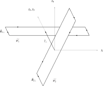
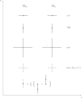
Figure 1: (Left) The relevant Wilson–loop configuration. Using the $O(4)$ invariance of the Euclidean theory we have put $\tilde{p}_{1}$ parallel to the $\tilde{x}_{1}$ axis. (Right) Loop configuration in the transverse plane.

In [7, 8] we have performed a Monte Carlo calculation of ${\cal G}_{L}$ for several values of the relative angle, various lengths and different configurations in the transverse plane. We used 30000 quenched configurations generated with the $SU(3)$ Wilson action at $\beta=6.0$, corresponding to $a\simeq 0.1\,{\rm fm}$, on a $16^{4}$ hypercubic lattice with periodic boundary conditions. This choice is made in order to stay within the so–called “scaling window”: in this sense we are relying in an indirect way on the validity of the relation (5) between Wilson–loop CFs on the lattice and in the continuum.

To keep the corrections due to $O(4)$ invariance breaking as small as possible, we have kept one of the two loops on–axis and we have only tilted the other one as shown in Fig. 1 (left). The on–axis loop $\widetilde{\cal W}_{L1}$ is taken to be parallel to the $x_{E1}$ axis, $\vec{l}_{1\parallel}=(L_{1},0)$, and of length $L_{1}=6,8$, and we have used two sets of off–axis loops $\widetilde{\cal W}_{L2}$ tilted at $\cot\theta=0,\pm 1,\pm 2$. We have used loops with transverse size $|\vec{r}_{1\perp}|=|\vec{r}_{2\perp}|=1$ in lattice units; the loop configurations in the transverse plane are those illustrated in Fig. 1 (right), namely $\vec{d}_{\perp}\parallel\vec{r}_{1\perp}\parallel\vec{r}_{2\perp}$ (which we call “zzz”) and $\vec{d}_{\perp}\perp\vec{r}_{1\perp}\parallel\vec{r}_{2\perp}$ (“zyy”). We have also measured the orientation–averaged quantity (“ave”) defined as ${\cal C}_{E}^{ave}(\theta;\vec{z}_{\perp};|\vec{R}_{1\perp}|,|\vec{R}_{2\perp}|)\equiv\int d\hat{R}_{1\perp}\int d\hat{R}_{2\perp}{\cal C}_{E}(\theta;\vec{z}_{\perp};\vec{R}_{1\perp},\vec{R}_{2\perp})$, where $\int d\hat{R}_{i\perp}$ stands for integration over the orientations of $\vec{R}_{i\perp}$. The lattice version of this equation is easily recovered for even (integer) values of the transverse sizes; in our particular case, $|\vec{r}_{i\perp}|=1$, we have to use a sort of “smearing” procedure, averaging nearby loops as depicted in Fig. 1 (right).

Since we are interested in the limit $T\to\infty$, we have to perform it on the lattice by looking for a plateau of ${\cal G}_{L}$ plotted against the loop lengths $L_{1,2}$. On a $16^{4}$ lattice it is difficult to have a sufficiently long loop while at the same time avoiding finite size effects, and at best we can push the calculation up to $L=8$. Nevertheless, our data show that ${\cal G}_{L}$ is already quite stable against variations of the loop lengths at $L_{1,2}\simeq 8$ (at least for $\theta$ not too close to $0^{\circ}$ or $180^{\circ}$, where it is expected to diverge due to its relation with the static dd potential, see [7, 8]) and so we can take the data for the largest loops available as a reasonable approximation of ${\cal C}_{L}$.

We have considered the values $d=0,1,2$ for the distance between the centers of the loops: as expected, the CFs vanish rapidly as $d$ increases, thus making the calculation with our simple “brute force” approach very difficult at larger distances.

4 Comparison with analytical results and the problem of total cross sections

As already pointed out in the Introduction, numerical simulations of LGT can provide the Euclidean CF only for a finite set of $\theta$–values, and so its analytic properties cannot be directly attained; nevertheless, they are first–principles calculations that give us (within the errors) the true QCD expectation for this quantity. Approximate analytic calculations of this same CF have then to be compared with the lattice data, in order to test the goodness of the approximations involved. This can be done either by direct comparison, when a numerical prediction is available, or by fitting the lattice data with the functional form provided by a given model. The Euclidean CFs we are interested in have been evaluated in the Stochastic Vacuum Model (SVM) [11], in the Instanton Liquid Model (ILM) [12, 8], and using the AdS/CFT correspondence [13]: the comparison of our data with these analytic calculations is not, generally speaking, fully satisfactory.

Figure 2: (Left) Comparison of the lattice data to the SVM expression (6), with $K_{\rm SVM}$ calculated according to [11] (solid line), or determined through a best–fit (for the “zzz” and “zyy” cases only, dotted line) at $d=1$. (Right) Comparison of the lattice data to the ILM expression (7) with $K_{\rm ILM}$ calculated according to [8] (dotted, dashed, and solid line, corresponding to different values of the model parameters), or determined through a best–fit (sparse dotted line) for the “zzz” and “zyy” cases at $d=1$.

In the SVM [11] the Wilson–loop CF is given by the expression

$${\cal C}^{\,\rm(SVM)}_{E}(\theta)=\frac{2}{3}\exp\left(-\frac{1}{3}K_{\rm SVM}\cot\theta\right)+\frac{1}{3}\exp\left(\frac{2}{3}K_{\rm SVM}\cot\theta\right)-1\,,$$ (6)

where $K_{\rm SVM}$ is a function of $\vec{z}_{\perp}$, $\vec{R}_{1\perp}$ and $\vec{R}_{2\perp}$ only, given in [11], that we have used to evaluate (6) numerically in the relevant cases. The SVM prediction (6) agrees with our lattice data in a few cases, at least in the shape and in the order of magnitude, but, in general, it is far from being satisfactory, see Fig. 2 (left). The same conclusion is reached if one performs instead a one–parameter ($K_{\rm SVM}$) best–fit with the given expression: the values of the chi–squared per degree of freedom ($\chi^{2}_{\rm d.o.f.}$) of this and the other fits that we have performed are listed in Table 1.

The ILM predicts the following functional form of the CF [12, 8],

$${\cal C}^{\,\rm(ILM)}_{E}(\theta)=\frac{K_{\rm ILM}}{\sin\theta}\,;$$ (7)

in particular, a well–defined numerical prediction for $K_{\rm ILM}$ has been obtained in [8]. The ILM prediction turns out to be more or less of the correct order of magnitude in the range of distances considered, at least around $\theta=\frac{\pi}{2}$, but it does not match properly the lattice data; the same mismatch is seen also in a best–fit with Eq. (7), see Fig. 2 (right). Moreover, the ILM prediction seems to overestimate the correlation length which sets the scale for the rapid decrease of the CF with the distance between the loops: this is also supported by the comparison of the prediction for the instanton–induced dd potential $V_{dd}$ with some preliminary numerical results on the lattice [8]. It is worth noting that largely improved best–fits (see Table 1) are obtained by combining Eq. (7) with the functional form ${\cal C}_{E}^{(\rm pert)}(\theta)=K_{\rm pert}(\cot\theta)^{2}$, corresponding to the leading–order result in perturbation theory [14, 4, 11], into the following expression, ${\cal C}^{\,\rm(ILMp)}_{E}(\theta)=\frac{K_{\rm ILMp}}{\sin\theta}+K_{\rm ILMp}^{\prime}(\cot\theta)^{2}$.

$\chi^{2}_{\rm d.o.f.}$	$d=0$		$d=1$			$d=2$
	zzz/zyy	ave	zzz	zyy	ave	zzz	zyy	ave
SVM	51	-	16	12	-	1.5	2.2	-
pert	53	34	16	13	13	1.5	2.2	4.5
ILM	114	94	14	15	45	0.45	0.35	1.45
ILMp	20	9.4	0.54	0.92	1.8	0.13	0.12	0.19
AdS/CFT	40	-	1	0.63	-	0.14	0.065	-

Table 1: Chi–squared per degree of freedom for a best–fit with the indicated function.

Finally, we have tried a best–fit with the expression obtained through AdS/CFT for the ${\cal N}=4$ SYM theory at large $N_{c}$, large ’t Hooft coupling and large distances between the loops [13]:

$${\cal C}^{\,\rm(AdS/CFT)}_{E}(\theta)=\exp\left\{\dfrac{K_{1}}{\sin\theta}+K_{2}\cot\theta+K_{3}\cos\theta\cot\theta\right\}-1\,.$$ (8)

Taking into account that it is a three–parameter best–fit, even this one is not satisfactory: best–fits with QCD–inspired expressions with only two parameters, like, e.g., the ILMp expression [or some appropriate modification of the SVM expression (6)] give smaller $\chi^{2}_{\rm d.o.f.}$ (see Table 1).

As an important side remark, we note that our data show a clear signal of $C$–odd contributions in dd scattering, which are related through the crossing–symmetry relations [5] to the antisymmetric part of ${\cal C}_{E}(\theta)$ with respect to $\theta=\frac{\pi}{2}$. An asymmetry is present in the “$zzz$” and “$zyy$” tranverse configurations (${\cal C}_{E}^{ave}$ is trivially symmetric), thus signalling the presence of odderon contributions to the dd scattering amplitudes. Although these $C$–odd contributions are averaged to zero in meson–meson scattering (at least in our model), they might play a non–trivial role in hadron–hadron processes in which baryons and antibaryons are also involved.

As we have said in the Introduction, the main motivation in studying soft high–energy scattering is that it can lead to a resolution of the total cross section puzzle. From this point of view, a satisfactory comparison of the lattice data with the SVM or the ILM would not have helped, since they yield constant or vanishing cross sections at high energy, as it can be seen by using Eqs. (3) and the optical theorem. An ambitious question that one can ask at this point is if the lattice data are compatible with rising total cross sections. An answer can in principle be obtained by performing best–fits to the lattice data with more general functions, leading to a non–trivial dependence on energy. This approach requires special care, because of the analytic continuation necessary to obtain the physical amplitude from the Euclidean CF: one has therefore to restrict the set of admissible fitting functions by imposing physical constraints (e.g., unitarity).

In this framework, a possible strategy is suggested by the improvement of best–fits achieved with the ILMp expression: the idea is to combine known QCD results and variations thereof. As an example, one could consider exponentiating two–gluon exchange and the one–instanton contribution (i.e., the ILMp expression), and supplementing it with a term which could yield a rising cross section, e.g., ${\cal C}_{E}^{\rm(rise)}=\exp\{{\cal C}_{E}^{\rm(ILMp)}\}\exp\{A_{\rm rise}(b)\left(\frac{\pi}{2}-\theta\right)^{4}(\cot\theta)^{2}\}-1$. Such an expression yields an amplitude respecting unitarity if $A_{\rm rise}(b)>0$ for large $b=|\vec{z}_{\perp}|$, and leads to the limit behaviour $\sim(\log s)^{2}$ allowed by the Froissart bound if $A_{\rm rise}(b)\sim b^{-4}$ for large $b$.

Another possible strategy is suggested by the AdS/CFT expression (8): one can try to adapt to the case of QCD the analytic expressions obtained in related models, such as ${\cal N}=4$ SYM. As it has been shown in [15], by combining the knowledge of the various coefficient functions $K_{i}$ in (8) at large $b$ [13] with the unitarity constraint in the small–$b$ region, a non–trivial high–energy behaviour for the dd total cross section in ${\cal N}=4$ SYM can emerge (including a pomeron–like behaviour $\sigma\sim s^{1/3}$). Although of course Eq. (8) is not expected to describe QCD, it is sensible to assume in this case a similar functional form (basically assuming the existence of the yet unknown gravity dual for QCD). Assuming moreover that the known power–law behaviour of the $K_{i}$’s (expected for a conformal theory) goes over into an exponentially damped one (expected for a confining theory), in particular $K_{3}\to ce^{-\mu b}$, one obtains a rising total cross section proportional to the limit behaviour $\sim(\log s)^{2}$.

It seems then worth investigating further the dependence of the CFs on the relative distance between the loops, as well as on the dipole sizes, as they could combine non–trivially with the dependence on the relative angle: these and other related issues (including the above–mentioned more general best–fits) are currently under study [16], and will be addressed in future works.

References

- [1] S. Donnachie, G. Dosch, P. Landshoff and O. Nachtmann, Pomeron Physics and QCD (Cambridge University Press, Cambridge, 2002).
- [2] O. Nachtmann, Ann. Phys. 209 (1991) 436.
- [3] E. Meggiolaro, Z. Phys. C 76 (1997) 523; Eur. Phys. J. C 4 (1998) 101; Nucl. Phys. B 625 (2002) 312.
- [4] E. Meggiolaro, Nucl. Phys. B 707 (2005) 199.
- [5] M. Giordano and E. Meggiolaro, Phys. Rev. D 74 (2006) 016003; E. Meggiolaro, Phys. Lett. B 651 (2007) 177.
- [6] M. Giordano and E. Meggiolaro, Phys. Lett. B 675 (2009) 123.
- [7] M. Giordano and E. Meggiolaro, Phys. Rev. D 78 (2008) 074510.
- [8] M. Giordano and E. Meggiolaro, Phys. Rev. D 81 (2010) 074022.
- [9] H.G. Dosch, E. Ferreira and A. Krämer, Phys. Rev. D 50 (1994) 1992.
- [10] J.E. Bresenham, IBM Sys. Jour. 4 (1965) 25.
- [11] A.I. Shoshi, F.D. Steffen, H.G. Dosch and H.J. Pirner, Phys. Rev. D 68 (2003) 074004.
- [12] E. Shuryak and I. Zahed, Phys. Rev. D 62 (2000) 085014.
- [13] R.A. Janik and R. Peschanski, Nucl. Phys. B 565 (2000) 193.
- [14] A. Babansky and I. Balitsky, Phys. Rev. D 67 (2003) 054026.
- [15] M. Giordano and R. Peschanski, JHEP 05 (2010) 037.
- [16] M. Giordano, E. Meggiolaro and N. Moretti, work in progress.