Paraglide: Interactive Parameter Space Partitioning for Computer Simulations

Abstract

In this paper we introduce paraglide, a visualization system designed for interactive exploration of parameter spaces of multi-variate simulation models. To get the right parameter configuration, model developers frequently have to go back and forth between setting parameters and qualitatively judging the outcomes of their model. During this process, they build up a grounded understanding of the parameter effects in order to pick the right setting. Current state-of-the-art tools and practices, however, fail to provide a systematic way of exploring these parameter spaces, making informed decisions about parameter settings a tedious and workload-intensive task. Paraglide endeavors to overcome this shortcoming by assisting the sampling of the parameter space and the discovery of qualitatively different model outcomes. This results in a decomposition of the model parameter space into regions of distinct behaviour. We developed paraglide in close collaboration with experts from three different domains, who all were involved in developing new models for their domain. We first analyzed current practices of six domain experts and derived a set of design requirements, then engaged in a longitudinal user-centered design process, and finally conducted three in-depth case studies underlining the usefulness of our approach.

1 Linking Formal and Real Systems

At the heart of computational science is the simulation of real-world scenarios. As it becomes possible to mimic increasingly comprehensive effects, it remains crucial to ensure a close correspondence between formal model and real system in order to draw any practically relevant conclusions. A well-established practical problem in this setting is the calibration of good parameter configurations that strengthen the fitness of the model [33, Ch. 1]. Even after matching model output with measured field data, there may still be free parameters that can be controlled to adjust the behaviour of the computer simulation. This can happen, if the expressive power of the model exceeds the number of available measurements, or if the measurements are so noisy that several different model instances are equally acceptable. In such a case, a domain expert could be involved to interactively tune free parameters of the model in order to favour solutions that match prior experience, theoretical insight, or intuition.

Towards that goal, we recognize that the optimization of parameters for some notion of performance is distinct from the objective to discover regions in parameter space that exhibit qualitatively different system behaviour, such as fluid vs. gaseous state, or formation of various movement patterns in a swarm simulation. Optimization is one focus of statistical methods in experimental design and has great potential for integration with visual tools, as for instance demonstrated recently by Torsney-Weir et al. [36]. The focus of this paper is on the latter aspect of qualitative discovery. This can support the understanding of the studied system, strengthen confidence in the suitability of the modelling mechanisms and, thus, become a substantial aid in the research process.

In the context of modelling this is a novel viewpoint, since typical approaches calibrate one best version of the model and then study how it behaves. To put regional parameter space exploration into practice, a number of challenges have to be overcome. To identify and address those, we (a) performed a field analysis of three application domains and derived a list of requirements, (b) present Paraglide, a system that addresses these requirements with a set of interaction and visualization techniques novel for this kind of application area, (c) conducted a longitudinal field evaluation of Paraglide showing practical benefits. In summary, Paraglide sets out to make the following contributions to computational modelling:

• Parameter region construction is promoted as a separate user interaction step during experimental design. This allows to address different efficiency issues of multi-dimensional sampling.

• A common step in explorative hypothesis formation is the construction of additional dependent feature variables and goal functions. Paraglide facilitates this with interpreter based back-ends. Also, this seamlessly integrates model code from sources such as MATLAB, R, or Python.

• Qualitatively distinct solutions are identified and the parameter space of the model is partitioned into the corresponding regions. This allows to visually derive global statements about the sensitivity of the model to parameter changes, which traditionally is studied locally.

2 Domain Characterization

In order to get a more detailed understanding of needs and requirements, we engaged in a problem characterization phase. We conducted contextual interviews with six experts from three different domains: engineering, mathematical modelling, and segmentation algorithm development. In the following, we characterize the investigated domains. Based on that, we summarize design requirements in Section 2.4 that are more general yet grounded in real-world application areas.

2.1 Mathematical Modelling: Collective behaviour in biological aggregations

Our first target group are two researchers studying properties of a mathematical model that describes biological aggregations. Furthering the understanding of such spatial and spatio-temporal patterns helps, for instance, to better predict animal migration behaviour. Modelled patterns can inform measures to contain plagues of locusts and positively affect quality of life in third world countries [7]. It may also help to better understand how, where, and when fish aggregations form and contribute to more efficient fishing strategies [29].

To study those spatio-temporal patterns, our participants developed a mathematical model [12, 23] consisting of a system of partial differential equations (PDEs) that express in one spatial dimension how left and right travelling densities of individuals move and turn over time. More details are given in the chapter notes. The basic idea is to take three kinds of social forces into account — namely attraction, repulsion, and alignment — that act globally among the densities of individuals. Attraction is the tendency between distant individuals to get closer to each other, repulsion is the social force that causes individuals in close proximity to repel from each other, and alignment represents the tendency to sync the direction of motion with neighbours. Solving the model for different choices of coefficients produces many complex spatial and spatio-temporal patterns observed in nature, such as stationary aggregations formed by resting animals, zigzagging flocks of birds, milling schools of fish, and rippling behaviour observed in Myxobacteria.

Our use case is part of a Master’s thesis on this subject with a focus on comparing two versions of their model. In the first one the velocity is constant. In the second one the individuals speed up or slow down as a response to their social interactions with neighbours. Comparing these models requires to solve them numerically for several different configurations. Each one of them corresponds to one specific choice of the $14$ model parameters, including the coefficients for the three postulated social forces. The output of the simulation is a spatio-temporal pattern of population densities. The number of basis functions that gives the resolution in space and time can be chosen to adjust the accuracy/runtime trade-off between $2$ minutes and an hour. With $5$ minutes each, one can perform a full computation of close to $300$ sample points in the duration of a single day.

To better understand the space of possible solutions, our participants manually explored the parameter combinations of their model and demonstrated its capability to reproduce a variety of complex patterns. While it is difficult to classify all possible patterns, there are a few standard solutions among them, for which established analysis techniques exist. In particular, they focus on the solutions of the system that do not change over time and space — so called spatially homogeneous steady states. A linear stability analysis of these steady states results in negative or positive growth rates for different perturbation frequencies, which respectively indicate stable and unstable solutions. There is a hypothesized relationship between the stability of steady states and the potential for pattern formation. This leads to a derived, more specific goal of the study. In particular, it allows to compare constant and non-constant velocity models by inspecting the change in shape of the parameter regions that lead to (un-)stable steady states. A discussion on how paraglide affects our participant’s workflow is given in Section 5.1.

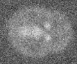
(a) raw data

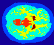
(b) ground truth

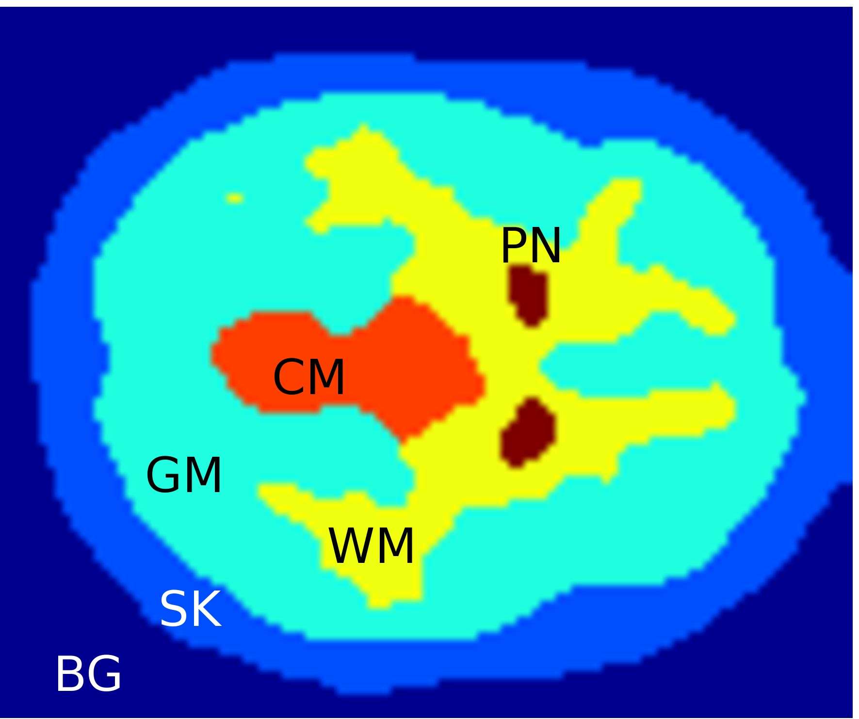
(c) config# 13, dice${}_{6}=.8136$

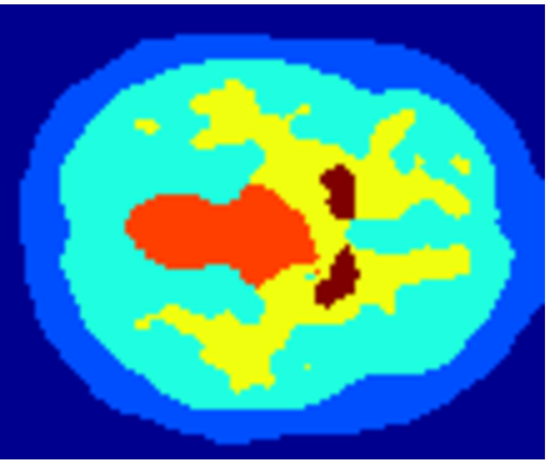
(d) config# 44, dice${}_{6}=.8128$

Figure 1: Classification of a slice of d-PET data using two different parameter configurations. The classes are 1: background (BG), 2: skull (SK), 3: grey matter (GM), 4: white matter (WM), 5: cerebellum (CM), and 6: putamen (PN).

2.2 Configuring a bio-medical image segmentation algorithm

Saad et al. [32] use a kinetic model to devise a multi-class, seed-initialized, iterative segmentation algorithm for molecular image quantification. Due to the low signal-to-noise ratio and partial volume effect present in dynamic-positron emission tomography (d-PET) data, their segmentation method has to incorporate prior knowledge. In this noisy setting, the segmentation of a basic random walker [14] would just result in Voronoi regions around the seed points. A new extension by Saad et al. makes this method usable for noisy data by adding energy terms that account for desirable criteria, such as data fidelity, shape prior, intensity prior, and regularization. In order to attain the superior segmentation quality of the algorithm, a proper choice of weights for the energy mixture is crucial.

To facilitate this choice of weight parameters, their code also provides numerical performance measures that assess the quality of each class. One such measure is the Dice coefficient [9], which gives a ratio of overlap with labelled training data. A second measure expresses an error of the quality of the kinetic modelling. Overall, the algorithm is influenced by $8$ factors or parameters. Ten response variables provide the $2$ quality measures per class, disregarding background.

Theoretically, the parameter calibration could proceed by numerical optimization of the performance with respect to the weights of the energy terms. However, for instance the Dice coefficients that indicate agreement of the segmented shape with given training data for putamen, using the two configurations of Figure 1(c) and (d), are both above the 90^th percentile of the sampled configurations and less than $0.003$ standard deviations apart. Numerically, this means that both segmentations are of the same, near optimal quality. Yet by visual inspection, it is possible to tell that the putamen (PN) shape in (d) is favourable over the one obtained in (c). Hence, guidance of a human domain expert is desirable to visually sort among several candidate solutions in order to find an improved segmentation, which is hard or impossible to choose automatically. An interactive workflow that facilitates such a procedure is subject of Section 5.2.

2.3 Engineering: Fuel cells

A fuel cell takes hydrogen and oxygen as gaseous input and converts them into water and heat, while generating an electric current. Affordable, high-performance fuel cells have the potential to enable more environmentally friendly means of transport by greatly reducing $\mathrm{CO_{2}}$ emissions. To manufacture a prototypical cell stack costs tens of thousands of dollars. Hence, a reliable synthetic model can greatly bring down the price of finding an optimal configuration for production.

The example investigated here is a simulation of a fuel cell stack developed by Chang et al. [8]. Their stack model is a system of coupled one-dimensional PDEs describing the individual cells in the stack. It can be adjusted with about $100$ parameters, where suitable choices of values are known for most of these parameters from fitting to available measurements. Computing a simulation run outputs $43$ different plots that show how certain physical quantities, such as current density, temperature, or relative humidity vary across the geometry of the cell stack. The computer model can be rerun for different configurations and, thus, allows for much broader exploration of design options than real prototyping. In particular, engineers are interested in varying different groups of parameters that represent the geometry of the assembly (size and number of cells in a stack), material properties (permeability), or running conditions (temperature, pressure, concentration) to study failure mechanisms and optimize performance. Experiments demonstrating the use of the suggested interactions are given in Section 5.3.

2.4 Problem structure

All previous use cases are motivated by questions about a real-worl system. In each setting, domain knowledge about the problem has been expressed in form of a computational model and the parameter space of the model is explored in order to relate observations about its properties to the corresponding real setting. The studies share a set of requirements as summarized in Figure 2.

• integrate with existing practices and code

• specify parameter region of interest (ROI)

• sample ROI and compute data set

• browse data providing overview (R3a) and detail (R3b)

• construct feature variables (assign manually or compute)

• combine features to derive a distance metric

• identify region(s) of similar outcome in parameter space

• find optimal point for a particular variable or user notion

• analyse sensitivity of feature values to change in input

• save state of the project for later reproduction

Figure 2: Summary of the requirement analysis.

Biological aggregation patterns: During our interviews, it became clear that it is important for these target users to inspect the behaviour of an existing MATLAB implementation for their PDE system (R1). This allows to invoke the simulation for different combinations of parameter values. Since multiple different parameter combinations have to be explored, it is necessary to narrow the computations down to suitable regions in parameter space (R2) and to assist the choice of sample points in these regions (R2a). Visual judgement of the computed solutions (R3) is one method to enable a qualitative distinction among different patterns of movement (R3b) and to determine which different sets of parameter choices produce a given behaviour (R3a and R5). The growth rate of a linear perturbation can be included as a feature variable (R4). Due to the size of the space of possible solutions, computational help to generate an overview of all possible behaviours would be desirable. To ensure findings are reproducible, it should be possible to save the state of the project (R8).

Bio-medical imaging: This use case is different from the others in that sampling and computation are not done by directly interfacing with the code, but rather are done offline to produce a data set for inspection. In this setting, assistance in choosing a suitable parameter region to sample is again an important task, where an interactive visual approach can be helpful (R2). Also, dependent feature variables (objective measures) are already constructed for segmentation quality (Dice coefficients) and kinetic modelling error. Requirements R1-3 apply here, except for the sample creation R2a. The comlexity of the segmentation problem can only be captured by multiple performance measures. The main goal is to find a robust parameter configuration that leads to good performance and is robust under a number of varying factors. In particular, performance should be invariant for different noise levels or patient scans. One step towards that goal is to produce a weighted sum of performance measures (R4). However, automatic optimization (R6) is challenging with multiple competing quality measures. For the algorithm to work robustly under different factors, it is important that the segmentation quality does not decay too quickly for slight changes to the chosen input parameter configuration (R7). To enable the user to assess robustness of a performance optimum, it is helpful to identify the region of parameter configurations that lead to ’good’ segmentation results (R3a+5), in order to make a robust choice within it.

Fuel cell stack design: This case of simulation model inspection invokes basic requirements R1-3. The goal of constructing a high-performance cell stack is akin to R4 and R6. Before that, however, the need to have a reliable and trusted model requires to identify parameter region boundaries that indicate transitions in stack behaviour. Such a decomposition into distinct parameter sets (R5) can greatly support reasoning about plausibility of the model.

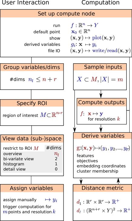
Figure 3: Abstraction of data, interaction, and computational components. Lines indicate shared data among processing steps and arrows prescribe an order of execution. On a more detailed level, Red is required input and blue denotes information that is available after a processing step.

2.5 Data abstraction

The conceptual organization of the required tasks is shown in Figure 3. It separately considers user interaction and computational pipeline, where all modules operate on the same data and share one flow of control. Integration with a computer simulation is possible using the compute node abstraction discussed in Section 4.1.

In order to accommodate simulations with a large number of variables $n+r$, a first step of the interaction allows the user to divide them into groups of smaller size $n_{l}$, e.g. separating input and output, or indicating other semantic information inherent to the simulation. The specification of a region of interest defines areas in the input space to sample and has further applications as detailed in Section 4.3.

In order to capture relationships among variables one can combine their domains using a Cartesian product and express a relation as a subset of this combined tuple data space. For a functional computer model $f(\mathbf{x})\mapsto\mathbf{y}$ one can further distinguish between input variables $(x_{1},x_{2},\dotsc,x_{n})=\mathbf{x}\in\mathbb{R}^{n}$ and output image $\mathbf{y}\in Y$. While meant in a mathematical sense, $\mathbf{y}$ can represent an actual picture or a disk image that captures the result of the computation. By application of another function it can be mapped into a Euclidean space $g:\mathbf{y}\mapsto(y_{1},y_{2},\dotsc,y_{r})\in\mathbb{R}^{r}$ of derived variables. The $x_{i}$ and $y_{i}$ are also referred to as factors and responses, respectively [41]. The inputs are often considered to be independent variables. However, this is not true in general, since the presence of constraints may introduce dependencies among the $x_{i}$.

Each configuration or data point $(\mathbf{x}_{k},g(\mathbf{y}_{k}))$ represents parameter input and output for a run of the simulation with all $m$ points combined forming the rows of a relational data table. The columns of this table represent the variables, which are synonymously refered to as dimensions. The variables that constitute input to the computation code are also referred to as parameters.

While the function $f$ is itself deterministic, uncertainties in the system can be modelled by providing additional environmental variables $x_{i}$ that are distributed according to some probability measure [34, p. 121]. We assume that code to compute $f$ is available as a black box that can be invoked for a finite number of points $X=\{\mathbf{x}_{k}\}$. This set $X$ is referred to as a design or a sample [34, p. 15]. Together with the mapping $f$ this allows to compute the responses $\{g\circ f(\mathbf{x}_{k})\}\subset\mathbb{R}^{r}$.

Depending on what derived variable $y_{i}=g_{i}(\mathbf{y})$ is specified (R4), its information may be interpreted as a feature, embedding coordinate, cluster membership label, likelihood for a model instance, distance from a template point, or objective measure — to give a few practical examples. In each case it may be possible to compute values or to assign them manually, depending on whether a function definition or a user’s concept is available. Some processing steps require a notion of distance or similarity among points. It can be obtained as Euclidean distance $d_{1}$ over combined feature vectors in $\mathbb{R}^{r}$. Beyond that, distance $d_{2}$ uses all information about each configuration point, including its parameter coordinates $\mathbf{x}\in\mathbb{R}^{n}$ or a domain specific function operating on the disk images.

3 Background

The following review will start with related systems that address certain requirements. Computational steering and experimental design will receive particular attention in this context. Methods specific to particular design aspects of paraglide will be discussed in the respective sections of Section 4.

3.1 Interactive environments for parameter adjustment in computer experiments

Computational steering considers adjustment of parameters during execution of time-dependent simulations [28]. Since our users do not modify parameters during the run of a simulation, our problem setting is different from classical steering in that we do not need to handle live updates of variables that are shared between simultaneously running modules. However, there is enough similarity to benefit from a comparison.

An evaluation of their computational steering environment (CSE) by Wijk et al. [40], recognizes major uses for debugging, presentation, and assistance in technical discussions that progress faster when ”What if?” questions can be answered immediately. A follow-up survey by Mulder et al. [28] identified further uses for model exploration, algorithm experimentation, and performance optimization. While these systems inspire numerous design decisions, the specific requirements for efficient regional sampling and an easy integration of end-user codes for simulation and derived variable computation are either not fulfilled or could be improved.

Berger et al. [1] discuss a system to visualize engineering and design options in the neighbourhood around an optimal configuration of a computer simulation. Based on a continuous function abstraction they provide a local analysis method that benefits domain experts. In order to not get stuck in local maxima, optimization methods usually benefit from an additional global perspective on the problem domain. The qualitative decomposition pointed out in the cases of Section 2 and pursued in the following provides such a complementary view.

The challenge of devising a user interaction for sample construction has recently been taken on in the Paranorama system of Pretorius et al. [31]. Their users can specify different ranges of interest for individual variables along with the number of requested distinct values per range. The sample points are then constructed via a Cartesian product of the value sets. Integrating this method into an image segmentation system, received positive feedback from users. However, combining many value ranges with this method may result in large sampling costs. Beyond numerical arguments, also screen space real estate is used up more quickly when viewing data sets with large numbers of variables, and a significantly increased cognitive cost arises when investigating and interpreting the effects of many factors on possibly multiple responses. Due to their significant impact on sampling and processing costs, Section 4.3 will give careful consideration to the number of involved variables and the volume of the region of interest.

3.2 Experimental Design

The task of generating a data set for a function $f$ has been abstracted in Section 2.5 as designing a sequence of points $\{\mathbf{x}_{k}\}=X\subset\mathbb{R}^{n}$ that discretize its domain. While there is a vast body of literature on the subject, the point of the following discussion is to provide a flavour of relevant issues and give entry points on how they are approached.

1. Exploratory designs: To facilitate a comprehensive analysis of the function $f$, a model of its full joint probability distribution $P\{X\leq\mathbf{x},Y\leq\mathbf{y}\}$ could be constructed [5, p.13], addressing R2a. To obtain such a complete model, a possible approach is to use space-filling designs.

2. Prediction-based designs: In order to compute a single aggregate statistic, such as the mean value of $f$, one can numerically perform integration, which amounts to the application of a linear functional. Further settings might involve the application of a family of such functionals, e.g. to approximate function values at new positions, which is also studied under the name of reconstruction or interpolation. In all of these settings it is possible to estimate an error or infer a confidence interval, which may or may not take newly acquired data into account.

3. Reconstruction model adjustment: To further adapt the reconstruction or regression model to field data, sample points are used to determine an appropriate model family (linear/non-linear), a suitably reduced dimensionality, or other regularization parameters. For instance, dimensional reduction and the choice of a correlation function for Gaussian Processes fall into this category.

4. Analyzing variability: Uncertainty analysis determines variability of a response based on the distributions given for the environmental variables, which provides confidence intervals for the responses that can be used to guide selection of relevant features [13]. Sensitivity analysis extends this analysis to determine how output variability is affected by each of the input variables [33] (R7). Similar measures appear in the analysis of (backward) stability of numerical algorithms [37, p. 104].

5. Optimization-based designs: In this setting, only those parts of the domain of $f$ are relevant that are likely to contain an optimum. Starting from an initial design, it is possible to steer concentration of the sample density in subsequent updates [25, 6, 20] (R6).

These tasks are somewhat ordered by decreasing degree of comprehensiveness. For instance, in the general case (1) will require an exhaustive sampling where (5) – after suitable initialization – may focus further points on small, promising regions in parameter space.

The book by Lemieux [22] gives an accessible overview on mostly non-adaptive (model-free) sampling methods that are for instance relevant to provide space-filling initializations for purposes 1, 2, or 4 in Section 3.2. Another exposition by Santner et al. [34] provides more background on model-adaptive sequential sampling, including an introduction to Gaussian process models (for purposes 2, 3, or 5), which are discussed more by Torsney-Weir et al. [36].

Of the above list, it will initially be aspect 1 that will matter in solving the problems laid out in Section 2. As more insight on the model behaviour is gained and included in the analysis, the adaptive techniques of categories 2 and 5 will address sampling requirements more effectively.

3.3 Parameter space partitioning

The computational model analysis cases of Section 2 all benefit from an overview of regions of distinct system behaviour marked out in their input parameter space (R5). There is no prior work in the academic visualization research that provides such a representation. However, after considering different names for the method, such as parameter space segmentation, clustering, or partitioning, it is the latter term that relates us to two prior contributions from an old and a recent member of the sciences, namely physics and psychology.

Bhatt and Koechling [4] study the behaviour during impact of two solid bodies with finite friction and restitution, which results in a tangential sliding velocity that continuously changes direction after impact. The problem is characterized by $9$ parameters, three for the impulse direction of the impacting body and six for its rotational moment of inertia tensor. The first step of their analysis determines a reduced set of three dimensionless parameters that completely define the tangential flow of sliding velocities. An important observation is that the qualitative behaviour of the flow is characterized by $2$ or $4$ solution curves of invariant direction, as well as the critical points and sign changes of the velocity along these straight lines. This results in $4$ main cases with up to $3$ sub-cases each. An implicit expression of the boundary between the cases is derived that is quartic in terms of the $3$ dimensionless parameters. By fixing one parameter and showing slices through this boundary, the enclosed regions can be visually distinguished and are labelled with the different cases they represent. This provides a comprehensive overview of all possible sliding behaviour. While providing a sophisticated algebraic analysis of a specific phenomenon, their discussion does not deal with numeric aspects involved of general computational models.

Pitt et al. [30] also promote parameter space partitioning and give an example analysis of a model that predicts, whether visual stimuli are recognized as words or non-words. In their overview of analysis techniques, they distinguish two axes that separate quantitative from qualitative and local from global techniques. In this view, partitioning is a global, qualitative method, and sensitivity analysis a case of more local, quantitative inspection.

Their method proceeds from a notion of equivalence among model configurations and a set of valid seed configuration points. The regions around these points are sampled using a Metropolis-Hastings algorithm with uniform target distribution. Rejected points have fallen into non-equivalent, adjacent regions and are explored subsequently.

An important point made by Pitt et al. is to also address the need to improve the user’s confidence in the plausibility of a given model. The studies they present are supported by showing the variety of qualitatively distinct model behaviour. However, a discussion of suitable analysis system design and considerations of required user interactions are not focus of their exposition.

3.4 Features to contribute

Methods to visually inspect multi-variate point distributions (to address R3a) are available in several of the frameworks listed earlier. However, the required capability to also generate data points (R2a) or to add derived dimensions (R4a) is missing from most systems that are mainly geared towards visualization of a static data set. Systems for experimental design, on the other hand, take care of the sampling requirements (R2a), but often lack interactive, visual methods to solicit required user input (R2). Computational steering systems combine sampling and visualization, but specifically focus on live-adjustments to parameters of a simulation that evolves over time. Their focus is often on some sort of interactive investigation, which could benefit from further support for broader state discovery (R5).

4 Design of the Paraglide system

We will now discuss aspects of the design of Paraglide, giving individual consideration to the graphical user interface (GUI), the software system, and choices of algorithms or methods for particular tasks. Paraglide was developed in a user-centered design process with five users, one or two from each domain. We met with our participants in person covering longitudinal time ranges of four years (fuel cell engineering), two years (mathematical modelling), with monthly meetings, and five months (image segmentation) with weekly meetings. In these meetings we discussed design mockups and prototypes, observed our users working with Paraglide, and gathered formative feedback in terms of usability and feature requests that we used to improve Paraglide’s design. In addition, these meetings contributed to refining our understanding of user practices and design requirements (see Section 2), as well as gathering summative feedback and anecdotal evidence (see Section 5).

Figure 4: Paraglide GUI running inside a MATLAB session to investigate the animal movement model of Section 2.1. Initially, deliberately chosen parameter combinations are imported from a switch/case script (a) by sampling the case selection variable of that script and recording the variables it sets. An overview (b) of the data is given in form of a scatter plot matrix (SPloM) for a chosen dimension group (h). Jython commands can be issued inside the command window (c) demonstrating the plug-in functionality of the system by manually importing the experiment module, which adds a new item to the menu bar (d). This allows to create a set of new sample points inside the region that is selected for parameters $q_{a}$ and $q_{al}$ (e). The configuration dialog for the MATLAB compute node (f) sets up a show command that produces a detail view of the spatio-temporal pattern (1D+time) (g). For the configuration point highlighted in yellow in the SPloM, this results in a pattern of two groups that merge and then progress upwards in a ’zigzag’ movement.

4.1 System components

The snapshot of Figure 4 shows the paraglide GUI and provides a brief overview of the main steps of the interaction. In the left of the main window (Figure 4d) dimension group tabs are shown that can be used to switch between selected subsets of variables. Right next to it appears the view for an individual group of dimensions (h), which shows histograms indicating the distribution of values for the respective variables. If a group has more than $8$ dimensions, compact range selectors are shown instead of histograms. This frees up screen space and eliminates computational costs for keeping their information updated, e.g. when the data set or the filtered selection changes. In Figure 4 the larger area in the right of the main window (d) provides a display of the data points (R2/a + R3a/b). In the example, a scatter plot matrix (SPloM) is shown (b) that arranges scatter plots on a grid, where each row or column is associated with one variable for the vertical or horizontal plot axes, respectively. Alternatively, it is possible to configure individual, enlarged scatter plots to inspect pairs of variables and show them in this area. In the console in (c) one can enter commands for MATLAB, Java, or the Jython interpeter that paraglide is running.

Workflow integration via scripting: Using the Jython import command to load modules readily takes care of managing dependencies among plug-ins. It is possible to script workflows at runtime and add them to the menu. Dependent scripts can be stored and recovered along with an XML description of the state of the current project. This also creates a separate folder that contains all cached disk images and other meta data.

Data management, view, control, and state: The core system is structured along the model–view–controller development pattern, which is partly inherited by using components of the prefuse system [16]. Particular use is made of the ability to select points of a centrally maintained prefuse table by evaluating a boolean expression on its row tuples with further details given in Section 4.3.

Compute node interface: To integrate domain specific computation code we use a ComputeNode abstraction. It can return a list of parameter names with optional description text and set/get accessors. A node may have more specialized features that it can announce internally by returning a list of capability descriptors. The main ones are compute solution, display plot, file IO, and compute feature, which in this order roughly correspond to the script lines that can be entered in the dialog of Figure 5. Respectively, this means the node may be able to provide different detail plots for a solution, it may compute solutions to a given configuration or derive named scalar or vector features, which are output quantities similar to plots. A node with file IO capability can store and retrieve cached solutions, such as MATLAB data files.

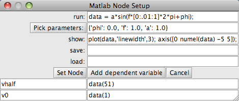
Figure 5: Dialog to set up a MATLAB compute node

The MATLAB node configuration dialog shown in Figure 5 is a simplified interface for the ComputeNode binding, where each of the edit boxes corresponds to one of the capabilities. In this particular example, the run command creates a sine wave $v_{t}=a\sin(ft2\pi+\phi)$ for $101$ values of $t=0\dotsc 1$, parameterized by phase shift $\phi$, frequency $f$, and amplitude $a$, with default values 0, 1, and 1, respectively. The show command displays the graph with axes of fixed height $\pm 5$. Due to instant computation, file IO is disabled.

The ’add dependent variable’ button allows to enter a line of code, whose return value is assigned to a variable of chosen name. This implements the derived variables $y_{i}=g(\mathbf{y})$ described in Section 2.5 and serves requirements R4/a. If a scalar is returned, it can be shown in the SPloM view along with the input variables. It is also possible to return vector features that may not be shown directly, but can be used to compute similarity or distance matrices, or to determine adjacency information. Methods to derive further embedding coordinates from this information are discussed in Section 4.3.4. The example in Figure 5 picks out the deflection of the oscillation at time $t=0$ ($v_{0}$) and half way into the interval ($v_{\frac{1}{2}}$). When inspecting these two ’features’, it becomes apparent that $v_{0}$ depends on $a$ and $\phi$ only, where $v_{\frac{1}{2}}$ is influenced by all three parameters. In this simple setting, it is possible to make this observation by thinking about the equation given for $v$, as well as by studying the scatter plots of input/output variable combinations. For the latter method, however, we would first need to create a data set of tuples $(a,f,\phi,v_{0},v_{\frac{1}{2}})$.

With a readily configured connection to the simulation back-end, Paraglide has a notion of the input parameter space $\mathbb{R}^{d}$ as well as the output space $\mathbb{R}^{k}$ of the simulation code. Initially, however, there may only be a single point of default values present, around which it is possible to expand the data set. To generate additional points it is possible to use some of the methods discussed in Section 3.2. While paraglide does not require to start with a given data set, the following discussion of system components will assume that an initial set of points already exists.

4.2 Browsing computed data

This stage provides the user with an overview of the data points as they distribute over input, output, and derived dimensions.

4.2.1 Viewing multi-dimensional data spaces

To address requirements R3a/b, we provide multiple simultaneous plots that give different views of the same data table and are linked to display a common focus point, highlight, or selection region. The subspaces that can be visualized that way range from multi- to 0-dimensional, to allow the user to relate overview of the whole distribution and detail plots that represent a single point. We also provide techniques to view 2D subspaces, such as scatter plots that allow for pair-wise inspection of relationships among variables, and 1D projections of the marginal densities that can be shown in form of histograms.

There are many more possible techniques for multi-variate multi-field data visualization, such as parallel coordinates, star plots, biplots, glyph-based visual encodings, or scatter plots arranged in a matrix or table layout, with discussions of pros and cons provided in various surveys [17, 11]. Implementations of these techniques are either contained directly in paraglide or are available via export to MATLAB, R, or protovis.

4.2.2 Grouping dimensions

As mentioned at the outset of this paper, the increased number of variables involved with modern simulation codes poses a challenge for their cognitive and numerical analysis. The visual complexity rises and makes data plots more difficult to interpret. The strategy of combining multiple views has its limits in screen space, as well as perceptual and cognitive handling. A possible remedy to this problem could be a) indirect visualization of fitted reduced dimensional models [17], or b) to divide the overall number of dimensions into groups for more focussed inspection.

Grouping simplifies complexity and can be based on statistical or structural information. Research on grouping of variables may consider dimension reduction and feature selection. To allow the user to express semantic information, we provide an interface to construct or modify a dimension group that simply consists of check boxes that indicate group membership for each variable. During browsing, only dimensions of the currently selected group are shown, which reduces the required screen space. While automatic assistance in forming these groups is imaginable, our current approach of manual selection proved sufficient in all use cases.

4.3 Specifying a region of interest

In the requirement analysis of Section 2 it became apparent that the specification of a region of interest (ROI) has multiple uses in different sub-tasks:

• specify a domain or sub-regions for sampling to create or refine the data set,

• choose a viewport to focus the overview,

• steer a cursor to set default values or invoke a detail view,

• make a selection of points for subset processing, for instance to manually assign labels,

• filter points to crop the viewed data range in order to deal with occlusion,

• enable mouse manipulation of the region description,

• export/import region descriptions to compare among different data sets.

4.3.1 Representing a region

Choosing a region of interest (ROI) and the construction of a set of sample points inside it, as described in 3.2, are tightly related. The shape of the region and a locally varying level of detail amount to support and density of a probability distribution. Seeing a finite set of sample points as discrete and a region description as continuous distribution, one can use distributional distance measures to assess how well one approximates the other.

While conceptually a probability distribution sufficiently describes what is needed to capture about a region of interest, it may be difficult for the user to grasp or specify, especially in multi-dimensional domains. A possible simplification is to omit the varying level of detail and to just consider uniform density. In this view the region is given by the support of the distribution and its volume corresponds to the inverse density. Defining more complex regions than hyper-boxes in Euclidean spaces of possibly more than three dimensions, however, is a complex task for a human user. An algebraic way to express what is wanted, as pursued with the feature definition language (FDL) of Doleisch et al. [10], can provide complementary input that goes beyond the expressive power of current interaction widgets. The XML encoding of paraglide’s system state includes a region description, which can be separately stored and imported.

4.3.2 Beyond the box — filtering derived variables

While this prior abstraction prepares much of what is needed in our application settings, the principal region template of a hyper-box might prove impractical in a higher-dimensional setting involving many variables. The reason for this lies in the drastic way the volume of a hyper-box rises relative to an inscribed 2-norm sphere as their dimensionality increases. This may not be much of a concern when selecting points from a given set. When generating samples, however, the costs are usually proportional to the volume of the requested region. So, ideally one would like to keep it as small as possible.

The degenerate form of a region shrunk to a single point constitutes a cursor. It can be used as a focus point for detail inspection, as well as a method to choose a default anchor for the generation of new samples. Starting from this, one way to obtain smaller regions simply amounts to a change in perspective from defining a region that covers certain value ranges to constructing a meaningful neighbourhood around the focus point. A common construct for such a point neighbourhood is a sphere bounded by some radius in a given metric.

This points to an alternative method of constructing custom regions by forming a hyper-box of ranges for chosen derived variables: For polytopes these would be linear combinations of other variables that make up the plane equations for the bounding facets. To obtain spheres in any metric, one could create a variable that measures the distance from a focus point. Bounding the maximum of this distance variable implicitly constructs a sphere on the dimensions that were involved in the distance computation. Boxes in this view are represented by the $\infty$-norm and a simple switch to the isotropic Euclidean $2$-norm sphere can significantly reduce the volume of interest. A data-adaptive example of dependent variables that facilitate, interactive multi-dimensional point selection is discussed in Section 4.3.4 and applied in Section 5.2.

4.3.3 User Interaction

The input method that we use to specify a region of interest is similar to prior approaches for constructing hyper-boxes. One of the first approaches is the HyperSlice system by van Wijk and van Liere [39]. They steer a multi-dimensional focus point by constraining its coordinates using multiple clicks that locate its position in different 2D projections that are presented in form of a scatter plot matrix. Martin and Ward [26] extend the possible user interactions to form a hyper-box shaped brushing region beyond scatterplot matrices to include parallel co-ordinates, or glyph views. The prosection matrix by Tweedie and Spence [38] also provides a similar form of control where the cursor point can be expanded into a hyper-box. The data inside the box is projected into different scatterplots. Collapsing an interval to a point changes the corresponding view from slab projection to slicing.

The previous interfaces map the data space to screen space using multiple axis aligned projections to $1$ or $2$-dimensional subspaces that map to range sliders or scatterplots. This requires the user to make a sequence of adjustments in order to specify a single cursor or region position. While this allows for a precise placement, the time required to make an adjustment grows at least linearly in the number of dimensions, while requiring the user to attend to multiple controls.

4.3.4 Non-linear screen mappings

One way to reduce the complexity of multi-dimensional cursor or region control is to reduce the number of involved linked projections. This could be achieved by providing views that give more comprehensive information about the data distribution than 2D projections. In particular, there is a family of techniques for non-linear screen space embeddings that are designed to reveal most characteristics of the data distribution. Enabling the user to make selections in such a view may obviate the need to consider views from other angles.

In these methods, each experimental run is again represented as a point, where spatial proximity among points corresponds to similarity of two runs. Point placement with respect to the coordinate axes is typically hard to interpret.

Prior work into this direction constructs slider widgets for smooth $n$-D parameter space navigation, as developed by Bergner et al.  [3] and by Smith et al. [35]. Both present a 2D embedding of sample nodes to obtain coordinates based on the screen distance between a movable slider and a set of nodes. Any curve the user describes by dragging the slider results in smoothly progressing weights that interpolate data at the nodes, which could result in different mixtures of light spectra or shape designs in the respective application setting.

Dimension reduction: Instead of arranging points in a circle or another prescribed shape, it is also possible to place them in a data adaptive way using dimension reduction techniques. Kilian et al. [21] use a distance preserving embedding of points to represent shape descriptors to control different designs of shapes. Jänicke et al. [19] lay out the minimum spanning tree of the data points for a multi-attribute point cloud, allowing the user to specify a region of interest in this embedding. Extending this to larger sets of points, the glimmer algorithm of Ingram et al. [18] is able to produce distance preserving embeddings for thousands of nodes via stochastic force computation on the GPU. Each of these methods require some notion of distance or adjacency among points, which is derived from dependent feature vectors that can be constructed through the interface described in Section 4.1.

Spectral embedding: To embed $m$ data points from an $n$-dimensional space to the $2$-D screen [24], we start from a data matrix $X\in\mathbb{R}^{m\times n}$. It can be turned into an affinity matrix $A=XX^{T}\in\mathbb{R}^{m\times m}$, whose elements are normalized as $(C)_{i,j}=(A)_{i,j}/\sqrt{(A)_{i,i}(A)_{j,j}}$ to yield a correlation matrix $C$. This implicitly scales each row-tuple in $X$ to lie on the surface of the $n$-dimensional $2$-norm unit sphere. Hence, the operation is referred to as sphering and the resulting elements of $C$ may be interpreted as cosine similarity or Pearson’s correlation coefficient. The orthogonal eigen-decomposition of this positive semi-definite matrix $C=VDV^{T}$ gives unit eigenvectors $\mathbf{v}_{i}=(V)_{:,i}$ with decreasing eigenvalues $\lambda_{i}=(D)_{i,i}$. The $m$ components of $\lambda_{2}\mathbf{v}_{2}$ and $\lambda_{3}\mathbf{v}_{3}$ are providing the $x$- and $y$-coordinates for the spectral embedding of the $m$ points, respectively.

Many variations of this technique are possible. Firstly, instead of constructing affinity $A$ via dot products, it is possible to employ any other monotonously decreasing kernel $(A)_{i,j}=\varphi(\mathbf{x}_{i},\mathbf{x}_{j})$, such as the Gaussian similarity kernel $\varphi(\mathbf{u},\mathbf{v})=\exp(-\lVert\mathbf{u}-\mathbf{v}\rVert^{2}/(2\sigma^{2}))$. Often, sphering is combined with a previous centering, where the mean $\boldsymbol{\mu}=X\cdot\mathbb{1}/n$ is subtracted from the data $X$. Alternatively, if the rows of $X$ contain frequencies or counts, one can rescale their sums to $1$, which projects the data points onto the surface of the positive orthant of the $1$-norm sphere.

The described method is dual to its popular ancestor — principle component analysis (PCA), where one instead begins with affinity $A=X^{T}X$ of centred data $X$. The above embedding algorithm then gives the $n$-dimensional principal components $\mathbf{v}_{i}$. When the data is projected onto an axis of direction $\mathbf{v}$ the variance of the resulting coefficients is $\sigma^{2}_{\mathbf{v}}=E_{X}[((\mathbf{x}-\boldsymbol{\mu})^{T}\mathbf{v})^{2}]=\mathbf{v}^{T}E_{X}[(\mathbf{x}-\boldsymbol{\mu})(\mathbf{x}-\boldsymbol{\mu})^{T}]\mathbf{v}=\mathbf{v}^{T}C\mathbf{v}$. This shows that the correlation matrix can be used to compute variance of the data for arbitrary axes and explains the special role of its dominant eigenvectors $\sigma^{2}_{\mathbf{v}_{i}}=\mathbf{v}_{i}^{T}C\mathbf{v}_{i}=\lambda_{i}$ to give directions of maximum variance. The different initializations of the data matrix lead to a family of techniques that include biplots, correspondence analysis, and (kernel-)PCA — all of them may be efficiently computed via singular value decomposition (SVD) [15].

Grouping points: Clusters of similar sample points can have arbitrary shapes. To not impose too strict assumptions on their distribution we opt for a manual method to assign cluster labels. For that, the user determines a plot where the clusters of interest are sufficiently separated. After enclosing the points by drawing rectangular regions in the plot, it is possible to manually assign cluster labels or to directly work with the multi-dimensional region description. Automatic clustering algorithms could perform poorly in this setting, if assumptions about cluster shape, such as convexity, are not met.

5 Validation in different use cases

In this section, we discuss qualitative feedback and anecdotal evidence from user interviews and usage sessions during the later stages of our user-centered design process (see Section 4). The first stable and iteratively improved versions of Paraglide were installed in the work environment of our three lead users. Overall, Paraglide has been in use at several occasions over a period of $4$ years, accompanied by weekly meetings of our research focus group for a period of $2$ years, and problem-adaptive meeting frequencies in the domain settings.

We present the summative findings in form of usage examples in which our users (a) were able to do something that they weren’t able to do without Paraglide, (b) could gather new insights into their model by using Paraglide, or (c) felt to be able to conduct some task more efficient with Paraglide than with traditional tools.

5.1 Movement patterns of biological aggregations

Semi-automatic screening for interesting solutions: In Section 2.1 a conjecture was pointed out that interesting spatial patterns only form with parameter configurations for which the PDE has unstable spatially homogenous steady states. This means that linear stability analysis of Section 2.1 can be used to detect the potential for pattern formation.

In the course of this research project, the model developer implemented a function to compute the type of (in-)stability for a given steady state. She had no problems to make the feature available in paraglide within few minutes using the compute node interface of Figure 5. Colouring the data points by stability type then helped to focus the pattern search, because computing the feature based on just the input $\mathbf{x}$ takes about $5$ seconds, where a full population density would take $5$ minutes per configuration point. With this computationally cheap screening, it became possible to cover larger areas of the parameter domain before zoning in on sub-areas to compute more comprehensive output that includes spatio-temporal patterns.

During one meeting a simple positivity test was implemented this way to answer, within five minutes, whether any solutions with negative densities were present — providing a very efficient debugging aid.

Discovering structure: To generate a set of sample points simply by specifying the containing region, the uniform sampling method, and the requested number of points, was considered a very convenient way to generate data: “You don’t need to worry about the coding, e.g. for loops, to set up region bounds, or choose sampling strategy.” Aside from saving time, the interaction also puts the user’s focus on core questions of choosing and combining value ranges. Within the selected range, coarse sampling to provide overview, followed by more focussed, finer sampling to acquire details, proved to be a good strategy — the structure in Figure 6 was found this way and inspired our user to further analytic investigation. In particular, that an increase in repulsion leads to increased stability and less pattern potential corresponds well with biological experience.

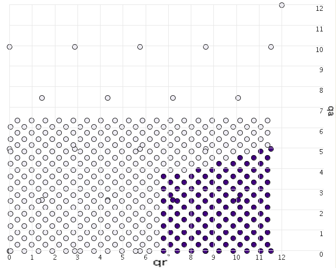
Figure 6: Illustrating the sample creation in a sub-region of the parameter space iterating from coarse to finer sampling. (Un-)filled circles indicate parameter configurations that lead to an (un-)stable steady state.

Investigating pattern formation hypothesis: To investigate the hypothesized relationship between pattern formation and linear stability analysis the customizable detail view feature proved helpful. The main output shows a full spatio-temporal pattern as given in Figure 4g. Another view created for this application is a bifurcation diagram that shows how the multiplicity and stability type of all steady states (spatially homogenous solutions of the PDE system) are changing, as one parameter ($q_{al}$ in this case) is changing its value. This enables further study of possible relationships between steady states and pattern formation, as shown in the supplementary video material.

Comparison of different model versions: The comparison of model versions using non-/constant velocities was enabled by creating two different feature variables computing the stability type using either of the two conditions. Switching the colour coding between these two variables allowed to visually compare the stability regions of the two model versions. This facilitated a main insight of the Master’s thesis, showing that the instability of most steady states tends to increase in the presence of non-constant velocities.

Overall, the users in this case found Paraglide to be: “a user-friendly tool that makes creating the sample points and comparing the computations much easier. This tool is capable of giving the user a better intuition about different solutions that correspond to various parameter configurations.”

5.2 Bio-medical imaging: Tuning Image Segmentation Parameters

In the following, we evaluate the use of paraglide in the context of Section 2.2. During three recorded meetings of overall $6$ hours a workflow was developed, implemented, and the required interaction steps performed. The goal there was to find a robust setting for eight parameters of a segmentation algorithm that produces good results for different data sets and noise levels, assessed by ten numeric objective measures. The term good in the sense of this discussion, refers to all points on a plateau of the optimization landscape that have target values close to the global optimum. When chosen from an initial, explorative sample they are also referred to as candidates, or representatives of the good cluster. Since the optimum is an ambiguous term in the context multi-objective optimization, our method proceeds by first grouping all points that are similar to each other. This leaves the task of finding out which cluster of points is a good one. The shape of the plateau of good points viewed in the space of input parameters informed the developer about which parameters to keep and which ones to drop. It also leads to a choice of configuration for the algorithm. To enable faster computation the volumetric patient data was reduced to a single slice that contains representatives from each class.

Find good candidate points by visual inspection: For easier inspection, the full set of variables is first broken down into groups. A SPloM view of the input parameters verified that the sampling pattern indeed uniformly covers the 2D scatterplot projections. To focus on the problem, the user isolated the group of performance measures described in Section 2.2. Manually chosen configuration points improved one or two performance criteria, and allowed to verify basic data sanity in a linked data table view. A combined manual optimization of the $2$ performance measures for each of the $5$ classes, however, would require to pay attention to simultaneous changes in $5$ scatterplots. The developer considered this a very difficult to infeasible task that needed to be simplified.

Construct the good neighbourhood: For most points in parameter space, a continuous change in the input parameters leads to a continuous change in the segmentation algorithm’s behaviour and the derived performance measures. This means that for each good point, it is worthwhile to explore the neighbourhood around it to find additional good and better settings [27]. With the distinction of input and output dimensions it is possible to construct and combine different notions of neighbourhood around a point. The dialog of Figure 5 is used to combine performance measures using weights that equalize the dynamic ranges. This feature vector space is then viewed using the spectral embeddings described in Section 4.3.4.

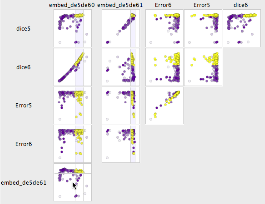
Figure 7: Scatter plot matrix view that compares the point embedding (lower left) with the objective measures that went into computing its underlying similarity measure. The numbering of the responses corresponds to the class labels of Figure 1.

Figure 7 shows the similarity embedding in the lower left view, where the good cluster is highlighted in yellow. Judging from the strong diagonal distribution in two plots in the matrix, the horizontal embedding dimension is dominated by dice6 and the vertical one by dice5. Since both should be maximized by good results, it is not surprising that manual inspection quickly identified the good cluster in the upper right of the embedding. The user found it convenient to make the cluster selection in the embedding, which underlines the point of Section 4.3.2. Apart from making interval selection easier, the embeddings also proved as an aid in a number of tasks: a) find good candidates, b) group adjacent good points into cluster(s), and c) check the embedding by inspecting it in a SPloM view together with the feature variables as in Figure 7.

Multi-factor assessment: To determine the relevance of each parameter for the overall performance of the segmentation algorithm, the developer viewed the distribution of the good cluster in input parameter space. This also gives a notion of sensitivity, where a large enough size of the good region indicates stability w.r.t. parameter changes [33, Sec. 1.2.3].

Figure 8: Scatter plot matrix view of the good cluster (yellow) identified in Figure 7 viewed in the subspace of input parameters. While sigma and alpha3 indicate clear thresholds beyond which the good configurations are found.

When projecting the cluster onto each variable individually, its shape can be either spread out or localized in one or multiple density concentrations. If the good points in the example of Figure 8 are spread out along a dimension, the corresponding parameter is unusable for steering between good and bad performance, as in this case for “don’t care” parameters alpha{1,2,7}. Observations like that inform the developer of energy terms to drop and, hence, directly influenced algorithm development. Parameters showing more localized good points or a clear transition are kept as part of the segmentation model and are set to some robust value that is further from the boundary, inside the good region.

Usage of the ROI representation: The region abstraction of Section 4.3 found application simplifying several tasks: a) inspect its content by transferring it between projects considering different segmentation noise level or patient data, b) to adjust the region description under these different experimental conditions, c) refine the sampling of configurations of the current model, d) communicate data requests via email. The main steps of the user driven optimization perform (a) and (b) iteratively for runs with different noise levels. This results in a region description for good and robust parameter choices. Refinement (c) was performed implicitly by applying (a) to a pre-computed denser data sample of $10,000$ points, which yielded $23$ good configurations with a segmentation quality similar to Figure 1d. The best chosen configuration of $\text{{\small\tt dice6}}=0.8282$ and $\text{{\small\tt error6}}=0.0621$, was also verified to be visually convincing.

Verify generalization: While the optimum has been made robust by constructing it over different experimental conditions, its performance has to generalize well beyond the condition used during adjustment. Hence, a final verification is run using data from $10$ previously unseen patients. Compared to the best configuration, the $10$ validation data sets showed very good Dice coefficient ($\mu=0.781540,\sigma=0.06$) and excellent kinetic modelling parameter error ($\mu=0.062,\sigma=0.0001$) throughout. This indicates that the configuration overall delivers high shape accuracy as well as low kinetic error. Two of the $10$ data sets yield just above average, yet acceptable, Dice coefficients, which inspired a separate investigation. This shows that the interaction steps suggested by paraglide can accelerate and benefit daily practice in state-of-the art research.

5.3 Fuel cell stack prototyping

The following case was introduced in Section 2.3 and concerns the simulation of a fuel cell stack. The model by Chang et al. [8] depends on about $100$ input parameters and produces $43$ different plots of various physical quantities characterizing the behavior of the cell stack. The parameters are structured into semantic groups describing different parts of the assembly. Further, the developer of the code has provided short description texts for the variables and their physical units. These parameter groups and descriptions are passed on through the ComputeNode interface of Section 4.1 and appear in paraglide as prepared variable groups and tool tips.

A parameter region of interest is chosen by the user, giving value ranges for the selected dimensions. All other parameters are kept at constant default values. Paraglide interfaces with the simulation code via a network connection, allowing multiple instances of the simulator to compute output for the generated sample configurations distributed over several computers. When all experiments are computed, one can choose an output plot of interest. The corresponding plots of all experiments are collected and compared using the correlation measure and layout method described at the end of Section 4.3.4. Since spatial proximity in these embeddings represents similarity in experimental outcome with respect to the chosen plot, detail inspection and manual labelling of multi-dimensional clusters using simple rectangle selection become feasible and improve confidence in the resulting decomposition.

(a) x-stack current, y-in temp.

(b) cell current density similarity

(c) MEA water content similarity

Figure 9: Two layouts for $204$ example experiments. a) input space showing variation in current and input temperature, b) embedding of the same samples where spatial proximity reflects plot similarity for cell current density, c) similarity embedding for membrane electrode assembly (MEA) water content using the same clusters as assigned in (b). Cluster representatives are shown in Figure 10 and Figure 11. These screenshots are from the 2007 C++ version of paraglide, and are also attainable in the currently discussed Java implementation.

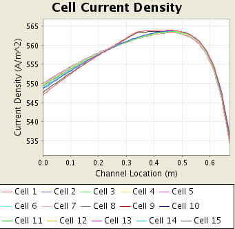
Figure 10: Cell current density plots for the clusters in Figure 9b

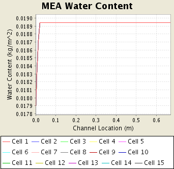
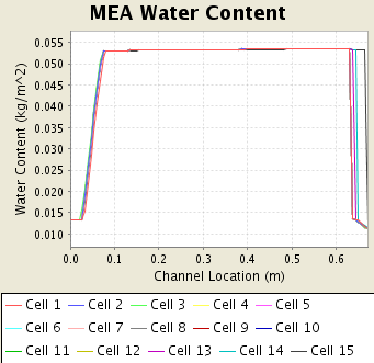
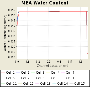
Figure 11: MEA water content plots for the clusters labelled in Figure 9c

Experiments with current and inflow temperature: To keep the initial experiment simple, we have chosen a region of interest over two input parameters: stack current ($10A..400A$) and stack inflow temperature ($333K..343K$). In this region $204$ samples are created with a uniform random distribution shown in Figure 9a. The color coding is added at a later stage and has no relevance for the initial step.

In Figure 9b the sample configurations are arranged according to their similarity in cell current density. In this embedding simulation outcomes can be inspected and configuration sample points can be manually labeled using a screen rectangle selection. For comparison, another similarity based embedding is shown in Figure 9c for the water content of the membrane-electrode assembly (MEA) using the same cluster labels as Figure 9b. When going back to the input space Figure 9a, the color coding reflects the parameter ranges of distinct behavior. Cluster representatives are shown in Figure 10 and Figure 11.

Our users found the parameter space partitioning of Figure 9 intriguing, giving them a new method to study their model. For instance, they pointed out that while cluster representative Figure 10e may be physically unreasonable, the (e) region in Figure 9a can be interpreted as a “bad” region, where adverse reactions occur.

6 Conclusion and Future Work

The development of computer simulations needs careful setup of the involved parameters. The discussed use cases indicated that the required understanding process can be time and resource intensive, and that systematic assistance is in order. Our validation of these investigations showed how the proposed decomposition of the continuous input parameter space benefits different questions. One finding suggests that even with potentially large numbers of variables, such a quantization can lead to a small number of regions. This can lead to a significant conceptual simplification and narrow down questions to particular sub-regions. Also, it provides starting points for local sensitivity analyses.

Future directions: Feasible or interesting regions for large numbers of variables can be relatively small in volume when compared to their bounding box. This is an example setting, where domain specific hints can help to guide the choice of sample points. For that, one could seek to obtain an implicit function representation of the region boundary, that could be used by the sampling module of Figure 3.

The region setup that has been identified as a requirement in several tasks, could consider navigation widgets for multi-dimensional parameter spaces. The aspects that have been investigated so far [3, 2] lead to interesting combinations of user interaction and dimension reduction.

The current implementation facilitates different point grouping methods: manual labelling, application of a classifier function, and clustering via a user determined similarity measure. Since clustering is key to parameter space partitioning, further research on suitable interactive and (semi-)automatic techniques for this purpose would be useful.

The investigated decomposition method results in a set of continuous regions. Considering this, initial research focussed on high-quality projection techniques for scatter plots of this kind of data. After adjusting research focus to sampling aspects and the use case evaluation presented here, suitable options to visually represent a region decomposition of a multi-dimensional continuous space still deserve further study.

References

- [1] W. Berger, H. Piringer, P. Filzmoser, and E. Gröller. Uncertainty-aware exploration of continuous parameter spaces using multivariate prediction. Computer Graphics Forum, 30(3):911–920, 2011.
- [2] S. Bergner, M. Crider, A. E. Kirkpatrick, and T. Möller. Mixing board versus mouse interaction in value adjustment tasks. Technical Report TR 2011-4, School of Computing Science, Simon Fraser University, Burnaby, BC, Canada, Sep 2011.
- [3] S. Bergner, T. Möller, M. Tory, and M. S. Drew. A practical approach to spectral volume rendering. IEEE Trans. on Vis. and Comp. Graphics, 11(2):207–216, March/April 2005.
- [4] V. Bhatt and J. Koechling. Partitioning the parameter space according to different behaviors during three-dimensional impacts. Journal of applied mechanics, 62:740, 1995.
- [5] C. M. Bishop. Pattern Recognition and Machine Learning. Springer, August 2006.
- [6] E. Brochu, N. D. Freitas, and A. Ghosh. Active preference learning with discrete choice data. In J. Platt, D. Koller, Y. Singer, and S. Roweis, editors, Advances in Neural Information Processing Systems 20, pages 409–416. MIT Press, Cambridge, MA, 2008.
- [7] J. Buhl, D. Sumpter, I. Couzin, J. Hale, E. Despland, E. Miller, and S. Simpson. From disorder to order in marching locusts. Science, 312(5778):1402, 2006.
- [8] P. Chang, G.-S. Kim, K. Promislow, and B. Wetton. Reduced dimensional computational models of polymer electrolyte membrane fuel cell stacks. J. Comput. Phys., 223(2):797–821, 2007.
- [9] L. R. Dice. Measures of the amount of ecologic association between species. Ecology, 26(3):297– 302, 1945.
- [10] H. Doleisch, M. Gasser, and H. Hauser. Interactive feature specification for focus+ context visualization of complex simulation data. In Proc. of the symposium on data visualisation 2003, pages 239–248. Eurographics Association, 2003.
- [11] M. Ferreira de Oliveira and H. Levkowitz. From visual data exploration to visual data mining: A survey. IEEE Trans. on Visualization and Computer Graphics, 9(3):378–394, 2003.
- [12] R. C. Fetecau and R. Eftimie. An investigation of a nonlocal hyperbolic model for self-organization of biological groups. J. Math. Biol., 61(4):545–579, 2010.
- [13] D. Francois. High-dimensional data analysis: optimal metrics and feature selection. PhD thesis, Université catholique de Louvain, 2007.
- [14] L. Grady. Random walks for image segmentation. IEEE Trans. on Pattern Analysis and Mach. Intelligence, 28(11):1768–1783, Nov. 2006.
- [15] M. Greenacre and T. Hastie. The geometric interpretation of correspondence analysis. J. of the Am. Stat. Assoc., 82(398):437–447, June 1987.
- [16] J. Heer and M. Agrawala. Software design patterns for information visualization. IEEE Trans. on Visualization and Computer Graphics, 12(5):853–860, 2006.
- [17] R. Holbrey. Data reduction algorithms for data mining and visualization. Technical report, University of Leeds/Edinburgh, 2006.
- [18] S. Ingram, T. Munzner, and M. Olano. Glimmer: Multilevel MDS on the GPU. IEEE Trans. on Visualization and Computer Graphics, pages 249–261, 2009.
- [19] H. Jänicke, M. Böttinger, and G. Scheuermann. Brushing of Attribute Clouds for the Visualization of Multivariate Data. IEEE Trans. on Visualization and Computer Graphics, 14(6):1459–1466, 2008.
- [20] D. Jones, M. Schonlau, and W. Welch. Efficient global optimization of expensive black-box functions. Journal of Global Optimization, 13(4):455–492, 1998.
- [21] M. Kilian, N. J. Mitra, and H. Pottmann. Geometric modeling in shape space. ACM Transactions on Graphics, 26(3):1–8, 2007.
- [22] C. Lemieux. Monte Carlo and Quasi-Monte Carlo Sampling. Springer Verlag, 2009.
- [23] F. Lutscher and A. Stevens. Emerging patterns in a hyperbolic model for locally interacting cell systems. J. Nonlinear Sci., 12:619–640, 2002.
- [24] U. Luxburg. A tutorial on spectral clustering. Statistics and Computing, 17(4):395–416, 2007.
- [25] J. Marks, B. Andalman, P. A. Beardsley, W. Freeman, S. Gibson, J. Hodgins, T. Kang, B. Mirtich, H. Pfister, W. Ruml, K. Ryall, J. Seims, and S. Shieber. Design galleries: A general approach to setting parameters for computer graphics and animation. In SIGGRAPH ’97, pages 389–400. ACM Press, 1997.
- [26] A. Martin and M. Ward. High dimensional brushing for interactive exploration of multivariate data. In Proc. of 6th Conference on Visualization ’95, pages 271–278. IEEE Computer Society, 1995.
- [27] C. Mcintosh and G. Hamarneh. Is a single energy functional sufficient? Adaptive energy functionals and automatic initialization. Proc. MICCAI, Part II, 4792:503– 510, 2007.
- [28] J. Mulder, J. van Wijk, and R. van Liere. A survey of computational steering environments. Future Generation Computer Systems, 15(1):119 – 129, 1999.
- [29] J. K. Parrish. Using behavior and ecology to exploit schooling fishes. Environ. Biol. Fish., 55:157–181, 1999.
- [30] M. Pitt, W. Kim, D. Navarro, and J. Myung. Global model analysis by parameter space partitioning. Psychological Review, 113(1):57, 2006.
- [31] A. Pretorius, M. Bray, A. Carpenter, and R. Ruddle. Visualization of parameter space for image analysis. IEEE Trans. on Vis. and comp. Graph., page In Press., 2011.
- [32] A. Saad, G. Hamarneh, T. Möller, and B. Smith. Kinetic modeling based probabilistic segmentation for molecular images. Medical Image Computing and Computer-Assisted Intervention–MICCAI 2008, pages 244–252, 2008.
- [33] A. Saltelli, M. Ratto, T. Andres, F. Campolongo, J. Cariboni, D. Gatelli, M. Saisana, and S. Tarantola. Global Sensitivity Analysis: The Primer. Wiley-Interscience, 2008.
- [34] T. Santner, B. Williams, and W. Notz. The Design and Analysis of Computer Experiments. Springer, 2003.
- [35] R. Smith, R. Pawlicki, I. Kókai, J. Finger, and T. Vetter. Navigating in a shape space of registered models. IEEE Trans. on Vis. and Comp. Graphics, pages 1552–1559, 2007.
- [36] T. Torsney-Weir, A. Saad, T. Möller, B. Weber, H.-C. Hege, J.-M. Verbavatz, and S. Bergner. Tuner: Principled Parameter Finding for Image Segmentation Algorithms Using Visual Response Surface Exploration. IEEE Trans. on Vis. and Comp. Graphics, pages ???–???, 2011.
- [37] L. Trefethen and D. B. III. Numerical Linear Algebra. SIAM, 1997.
- [38] L. Tweedie and R. Spence. The prosection matrix: A tool to support the interactive exploration of statistical models and data. Computational Statistics, 13(1):65–76, 1998.
- [39] J. van Wijk and R. van Liere. HyperSlice: Visualization of scalar functions of many variables. In Proc. of 4th Conf. on Visualization’93, pages 119–125. IEEE Computer Society, 1993.
- [40] J. van Wijk, R. Van Liere, and J. Mulder. Bringing computational steering to the user. In Scientific Visualization Conference, 1997, pages 304–304. IEEE, 1997.
- [41] P. Wong and R. Bergeron. Years of Multidimensional Multivariate Visualization. Scientific Visualization, Overviews, Methodologies, and Techniques, pages 3–33, 1994.